An Unbiased Predictor for Skewed Response Variable with Measurement Error in Covariate

Abstract

We introduce a new small area predictor when the Fay-Herriot normal error model is fitted to a logarithmically transformed response variable, and the covariate is measured with error. This framework has been previously studied by Mosaferi et al. (2023). The empirical predictor given in their manuscript cannot perform uniformly better than the direct estimator. Our proposed predictor in this manuscript is unbiased and can perform uniformly better than the one proposed in Mosaferi et al. (2023). We derive an approximation of the mean squared error (MSE) for the predictor. The prediction intervals based on the MSE suffer from coverage problems. Thus, we propose a non-parametric bootstrap prediction interval which is more accurate. This problem is of great interest in small area applications since statistical agencies and agricultural surveys are often asked to produce estimates of right skewed variables with covariates measured with errors. With Monte Carlo simulation studies and two Census Bureau’s data sets, we demonstrate the superiority of our proposed methodology.

Key words and phrases: Bayes estimator, prediction interval, transformation.

Introduction

Small area estimation concerns producing estimates or predictions of means, totals or quantiles for each of a finite collection of geographic regions, where there are a small number of sampled units in each individual region (area). Classical models used in small area estimation take the form of mixed linear models that result from the concatenation of a model for error in direct sample-based estimators for each area and an additional model that connects areas through the use of covariates and area-specific random effects.

These linking models take the direct estimators to be linear combinations of covariates and random effects. We focus here on what is called the area level model (Ghosh and Rao (1994), Pfefferman (2013), and Rao and Molina (2015), Chap. 4) which uses covariates at the level of the areas. Recently, Mosaferi et al. (2023) proposed a model of the Fay-Herriot type and developed an empirical predictor for small area quantities that they are right skewed.

A complication that arises is that the area-level covariates to be used can be the result of survey sampling (see for instance Ybarra and Lohr (2008)), thus producing a small area model with measurement error in the covariates. The predictor given in their manuscript cannot perform uniformly better than the direct estimator because of bias issues. In this manuscript, we propose a new unbiased predictor, which can perform uniformly better than that of Mosaferi et al. (2023) and the direct estimator.

Much work with small area models has been devoted to the estimation of MSE. Prasad and Rao (1990) derived a closed form approximation for the estimator of the MSE of an empirical Bayes (EB) predictor under the assumption of normality. Jiang et al. (2002) proposed a jackknife estimator based on a decomposition of MSE where the leading term is approximately unbiased and does not depend on the area-specific random effects. Butar and Lahiri (2003) developed a bootstrap estimator of MSE.

Here, we derive an approximation of the MSE for the predictor as well as the jackknife estimator of MSE. Prediction intervals based on these suffer from inadequate coverage probabilities. In order to address this shortcoming, we develop prediction intervals based on a non-parametric bootstrap method. In the rest of this section, we list some of the previous works in the literature and highlight our contributions.

Prior Work

Molina and Martín (2018) and Berg and Chandra (2014) worked on the log-transformation model and proposed an EB predictor for the value of the variable of interest for out-of-sample individuals (and for small area means) in a nested-error regression model where no measurement error is assumed present in the covariates. The analytical MSE given in Molina and Martín (2018) has a complex form. Thus, the authors proposed a parametric bootstrap procedure for estimation of the uncertainty following Butar and Lahiri (2003). Slud and Maiti (2006) proposed a large sample approximation to the MSE of the predictor for the transformed Fay-Herriot model without measurement error.

Our Contributions

In this paper, we make several contributions to the literature. First, unlike the earlier works given in Section 1.1, we assume the available covariate in the model is measured with error. Second, we propose a new small area predictor for the skewed response variable in the original scale at the area-level instead of unit-level under presence of measurement error in covariate and make comparisons with the earlier predictor proposed by Mosaferi et al. (2023). Third, we explain how to estimate the unknown parameters using unbiased score functions from the marginal likelihood. Finally, we derive an approximation for the MSE of our proposed predictor and develop prediction intervals based on nonparametric bootstrap techniques.

The rest of the paper is organized as follows. In Section 2, we apply the Fay and Herriot (1979) model to the transformed data with measurement error in covariate and formulate the problem. In Section 3, we derive a new predictor for the response variable in the proposed modeling framework. In Section 4, we explain how to estimate the unknown parameters in the model. In Section 5, we derive an estimator of the MSE of the predictor.

In Section 6, we construct non-parametric bootstrap prediction intervals. In Section 7, using a Monte Carlo simulation study, we make comparisons with other predictors given in the literature. In Section 8, we illustrate our methodology using two data sets from the Census Bureau. The related discussions and possible extensions are given in Section 9. Technical details and additional numerical results are in the Supplementary Material. All the R code implementing the proposed methodology is available at Github repository https://github.com/SepidehMosaferi/UnbiasedPredictor_SkewedData.

Transformed Fay-Herriot Model with Measurement Errors

Assume response variables $y_{i}$ ($i=1,...,m$) are right skewed. Thus, the log transformation of $y_{i}$ can stabilize the variation. Let $z_{i}=\log(y_{i})$ and $z_{i}=\phi_{i}+e_{i}$, where $\phi_{i}=\log(\theta_{i})$ such that $\theta_{i}$ is unknown and $e_{i}\overset{\text{ind}}{\sim}N(0,\psi_{i})$ is the sampling error. We further define $\phi_{i}=\beta_{0}+\beta_{1}x_{i}+v_{i}$, where the covariate $x_{i}$ is not observed, and what one observes is the $W_{i}$. The linking error is $v_{i}\overset{\text{iid}}{\sim}N(0,\sigma^{2}_{v})$. The error terms ($e_{i},v_{i}$) are mutually independent per each $i$-th small area.

Then, the transformed Fay-Herriot model with measurement error in covariate can be presented with the following hierarchical set-up

$$z_{i}|\phi_{i} \overset{\text{ind}}{\sim}N(\phi_{i},\psi_{i})$$

$$\phi_{i} \overset{\text{ind}}{\sim}N(\beta_{0}+\beta_{1}x_{i},\sigma^{2}_{v})$$

$$W_{i} \overset{\text{ind}}{\sim}N(x_{i},C_{i}),\quad i=1,...,m.$$ (2.1)

The $(z_{i},\phi_{i})$ are assumed to be independent of the $W_{i}$. This is because the former constitutes the sampling and linking model, while the later brings in the measurement error part. Here, following Ybarra and Lohr (2008), $\sigma^{2}_{v}$ is unknown but the sampling variances $\psi_{i}$ and $C_{i}$ are assumed to be known, which can be obtained from the asymptotic variances of transformed direct estimates (see, Carter and Rolph (1974), Efron and Morris (1975), and Fay and Herriot (1979)).

The primary parameter of interest in the original scale is $\theta_{i}\equiv\exp(\beta_{0}+\beta_{1}x_{i}+v_{i})$. Prediction of $\phi_{i}=\log(\theta_{i})$, where $\log(\theta_{i})\equiv\beta_{0}+\beta_{1}x_{i}+v_{i}$, is identical to the problem of Ybarra and Lohr (2008).

We will adopt an empirical Bayes approach for estimation of the $\theta_{i}$. We will assume a flat prior for all the $x_{i}$’s, but then estimate $\beta_{0}$, $\beta_{1}$, and $\sigma^{2}_{v}$ from the resulting marginal likelihood. To this end, first observe that writing $\gamma^{\star}_{i}=\sigma^{2}_{v}/(\sigma^{2}_{v}+\psi_{i})$, the conditional posterior distributions

$$\phi_{i}|\beta_{0},\beta_{1},\sigma^{2}_{v},x_{i},z_{i},W_{i}\overset{\text{ind}}{\sim}N(\gamma^{\star}_{i}z_{i}+(1-\gamma^{\star}_{i})(\beta_{0}+\beta_{1}x_{i}),\gamma^{\star}_{i}\psi_{i}),$$

and $x_{i}|\beta_{0},\beta_{1},\sigma^{2}_{v},z_{i},W_{i}$ are mutually independent, where

$$\pi(x_{i}|\beta_{0},\beta_{1},\sigma^{2}_{v},z_{i},W_{i})\propto(\sigma^{2}_{v}+\psi_{i})^{-1/2}\exp\Big{[}-\frac{1}{2}\Big{\{}\frac{(z_{i}-\beta_{0}-\beta_{1}x_{i})^{2}}{\sigma^{2}_{v}+\psi_{i}}+\frac{(W_{i}-x_{i})^{2}}{C_{i}}\Big{\}}\Big{]}.$$

Next we use the identity,

$$(z_{i}-\beta_{0}-\beta_{1}x_{i})^{2}/(\sigma^{2}_{v}+\psi_{i})+(W_{i}-x_{i})^{2}/C_{i}=\{\beta_{1}^{2}C_{i}+\sigma^{2}_{v}+\psi_{i}\}^{-1}\times(z_{i}-\beta_{0}-\beta_{1}W_{i})^{2}$$

$$\quad+\{\beta_{1}^{2}/(\sigma^{2}_{v}+\psi_{i})+C_{i}^{-1}\}\times\Big{(}x_{i}-\Big{\{}\frac{\beta_{1}(z_{i}-\beta_{0})}{\sigma^{2}_{v}+\psi_{i}}+\frac{W_{i}}{C_{i}}\Big{\}}\Big{/}\Big{\{}\frac{\beta_{1}^{2}}{\sigma^{2}_{v}+\psi_{i}}+\frac{1}{C_{i}}\Big{\}}\Big{)}^{2}.$$ (2.2)

Now writing $S_{i}(\beta_{1},\sigma^{2}_{v})=\beta_{1}^{2}C_{i}+\sigma^{2}_{v}+\psi_{i}$, one gets

$$x_{i}|\beta_{0},\beta_{1},\sigma^{2}_{v},z_{i},W_{i}\overset{\text{ind}}{\sim}N\Big{[}\frac{\beta_{1}C_{i}(z_{i}-\beta_{0})+(\sigma^{2}_{v}+\psi_{i})W_{i}}{S_{i}(\beta_{1},\sigma^{2}_{v})},\frac{\sigma^{2}_{v}+\psi_{i}}{S_{i}(\beta_{1},\sigma^{2}_{v})}\Big{]}.$$

Accordingly,

$$E(\phi_{i}|\beta_{0},\beta_{1},\sigma^{2}_{v},z_{i},W_{i}) =E\Big{[}E(\phi_{i}|\beta_{0},\beta_{1},\sigma^{2}_{v},x_{i},z_{i},W_{i})|\beta_{0},\beta_{1},\sigma^{2}_{v},z_{i},W_{i}\Big{]}$$

$$=\frac{\sigma^{2}_{v}}{\sigma^{2}_{v}+\psi_{i}}z_{i}+\frac{\psi_{i}}{\sigma^{2}_{v}+\psi_{i}}\Big{[}\beta_{0}+\beta_{1}\Big{\{}\frac{\beta_{1}C_{i}(z_{i}-\beta_{0})+(\sigma^{2}_{v}+\psi_{i})W_{i}}{S_{i}(\beta_{1},\sigma^{2}_{v})}\Big{\}}\Big{]}$$

$$=\frac{\sigma^{2}_{v}\,S_{i}(\beta_{1},\sigma^{2}_{v})+\psi_{i}\beta_{1}^{2}C_{i}}{(\sigma^{2}_{v}+\psi_{i})S_{i}(\beta_{1},\sigma^{2}_{v})}z_{i}+\frac{\psi_{i}}{\sigma^{2}_{v}+\psi_{i}}\Big{[}\frac{\beta_{0}(\sigma^{2}_{v}+\psi_{i})}{S_{i}(\beta_{1},\sigma^{2}_{v})}+\frac{\beta_{1}(\sigma^{2}_{v}+\psi_{i})W_{i}}{S_{i}(\beta_{1},\sigma^{2}_{v})}\Big{]}$$

$$=\frac{\beta_{1}^{2}C_{i}+\sigma^{2}_{v}}{S_{i}(\beta_{1},\sigma^{2}_{v})}z_{i}+\frac{\psi_{i}(\beta_{0}+\beta_{1}W_{i})}{S_{i}(\beta_{1},\sigma^{2}_{v})}=\tilde{\gamma}_{i}z_{i}+(1-\tilde{\gamma}_{i})(\beta_{0}+\beta_{1}W_{i}),$$

where $\tilde{\gamma}_{i}\equiv(\beta_{1}^{2}C_{i}+\sigma^{2}_{v})/S_{i}(\beta_{1},\sigma^{2}_{v})$. Further,

$$V(\phi_{i}|\beta_{0},\beta_{1},\sigma^{2}_{v},z_{i},W_{i}) =E\Big{[}V(\phi_{i}|\beta_{0},\beta_{1},\sigma^{2}_{v},x_{i},z_{i},W_{i})|\beta_{0},\beta_{1},\sigma^{2}_{v},z_{i},W_{i}\Big{]}$$

$$\quad+V\Big{[}E(\phi_{i}|\beta_{0},\beta_{1},\sigma^{2}_{v},x_{i},z_{i},W_{i})|\beta_{0},\beta_{1},\sigma^{2}_{v},z_{i},W_{i}\Big{]}$$

$$=\gamma_{i}^{\star}\psi_{i}+(1-\gamma_{i}^{\star})^{2}\beta_{1}^{2}\frac{(\sigma^{2}_{v}+\psi_{i})C_{i}}{S_{i}(\beta_{1},\sigma^{2}_{v})}$$

$$=\frac{\sigma^{2}_{v}\psi_{i}}{\sigma^{2}_{v}+\psi_{i}}+\frac{\psi_{i}^{2}}{(\sigma^{2}_{v}+\psi_{i})^{2}}\beta_{1}^{2}C_{i}\frac{\sigma^{2}_{v}+\psi_{i}}{S_{i}(\beta_{1},\sigma^{2}_{v})}$$

$$=\frac{1}{\sigma^{2}_{v}+\psi_{i}}\Big{[}\sigma^{2}_{v}\psi_{i}+\frac{\psi_{i}^{2}\beta_{1}^{2}C_{i}}{S_{i}(\beta_{1},\sigma^{2}_{v})}\Big{]}$$

$$=\frac{\psi_{i}}{(\sigma^{2}_{v}+\psi_{i})S_{i}(\beta_{1},\sigma^{2}_{v})}\Big{[}\sigma^{2}_{v}(\beta_{1}^{2}C_{i}+\sigma^{2}_{v}+\psi_{i})+\beta_{1}^{2}C_{i}\psi_{i}\Big{]}$$

$$=\frac{\psi_{i}}{(\sigma^{2}_{v}+\psi_{i})S_{i}(\beta_{1},\sigma^{2}_{v})}\Big{[}\sigma^{2}_{v}(\sigma^{2}_{v}+\psi_{i})+\beta_{1}^{2}C_{i}(\sigma^{2}_{v}+\psi_{i})\Big{]}=\tilde{\gamma}_{i}\psi_{i}.$$

This leads to the Bayes estimator

$$\tilde{\theta}_{i,A} =E[\exp(\phi_{i})|\beta_{0},\beta_{1},\sigma^{2}_{v},z_{i},W_{i}]$$

$$=\exp(\tilde{\gamma}_{i}z_{i}+(1-\tilde{\gamma}_{i})(\beta_{0}+\beta_{1}W_{i})+\tilde{\gamma}_{i}\psi_{i}/2),$$

proposed by Mosaferi et al. (2023). Also,

$$V[\exp(\phi_{i})|\beta_{0},\beta_{1},\sigma^{2}_{v},z_{i},W_{i}] =\exp\{\tilde{\gamma}_{i}\psi_{i}\}[\exp\{\tilde{\gamma}_{i}\psi_{i}\}-1]$$

$$\quad\times\exp\{2[\tilde{\gamma}_{i}z_{i}+(1-\tilde{\gamma}_{i})(\beta_{0}+\beta_{1}W_{i})]\}.$$

Further, from (2), the marginal likelihood of $(\beta_{0},\beta_{1},\sigma^{2}_{v})$ is given by

$$L_{M}(\beta_{0},\beta_{1},\sigma^{2}_{v})=\prod_{i=1}^{m}S_{i}^{-1/2}(\beta_{1},\sigma^{2}_{v})\,\exp\Big{[}-\frac{1}{2}\sum_{i=1}^{m}\frac{\tau_{i}^{2}(\beta_{0},\beta_{1})}{S_{i}(\beta_{1},\sigma^{2}_{v})}\Big{]},$$ (2.3)

where we define $\tau_{i}(\beta_{0},\beta_{1})=z_{i}-\beta_{0}-\beta_{1}W_{i}$. In the reminder of this paper, we will work with the score functions based on the marginal likelihood (2.3) to estimate the vector of unknown parameters.

Optimal Predictor in the Original Scale

It is clear that $E(\tilde{\theta}_{i,A})=E(\theta_{i})=\exp(\beta_{0}+\beta_{1}x_{i}+\frac{1}{2}\sigma^{2}_{v})$ when $C_{i}=0$. The above equality, however, is not true in general. To this end, we prove the following theorem.

Theorem 1.

$E(\tilde{\theta}_{i,A})=\exp(\beta_{0}+\beta_{1}x_{i}+\frac{1}{2}\{\tilde{\gamma}_{i}(\sigma^{2}_{v}+\psi_{i})+(1-\tilde{\gamma}_{i})\beta_{1}^{2}C_{i}\})$.

Proof: See Supplementary Material.

In view of Theorem 1,

$$\frac{E(\tilde{\theta}_{i,A})}{E(\theta_{i})} =\exp\Big{(}\frac{1}{2}\{\tilde{\gamma}_{i}(\sigma^{2}_{v}+\psi_{i})+(1-\tilde{\gamma}_{i})\beta_{1}^{2}C_{i}-\sigma^{2}_{v}\}\Big{)}$$

$$=\exp\Big{(}\frac{1}{2}d_{i}\Big{)},\quad\text{(say)}$$

that is

$$E\Big{\{}\tilde{\theta}_{i,A}\exp\Big{(}-\frac{1}{2}d_{i}\Big{)}\Big{\}}=E(\theta_{i}).$$

Therefore, our proposed unbiased predictor is

$$\tilde{\theta}_{i,B}=\tilde{\theta}_{i,A}\exp\Big{(}-\frac{1}{2}\,d_{i}\Big{)}.$$ (3.1)

With some algebra, $d_{i}$ can be simplified as $d_{i}=2\psi_{i}\beta_{1}^{2}C_{i}/S_{i}(\beta_{1},\sigma^{2}_{v})$.

Remark 1.

When $C_{i}=0$, the true value of $x_{i}$ can be used for the optimal predictor. By substituting $C_{i}=0$ into $\tilde{\theta}_{i,B}$, the optimal predictor is $\tilde{\theta}_{i,B}^{0}=\exp(\gamma_{i}^{\star}z_{i}+(1-\gamma_{i}^{\star})(\beta_{0}+\beta_{1}x_{i})+\gamma_{i}^{\star}\psi_{i}/2)$, which is same as the predictor given in Slud and Maiti (2006) and is also identical to predictor $\tilde{\theta}_{i,A}$.

Estimating the Unknown Parameters

We are interested in obtaining estimates of the vector of unknown parameters $\bm{\omega}=(\beta_{0},\beta_{1},\sigma^{2}_{v})^{\prime}$. Note that we do not directly use the partial derivatives of the marginal likelihood given in expression (2.3) since they are not unbiased. We denote the log-likelihood of $L_{M}(.)$ in (2.3) by $\ell_{M}(\bm{\omega})$. The score functions of $\ell_{M}(\bm{\omega})$ can be defined as follows:

$$U(\bm{\omega})=(U_{1}(\bm{\omega}),U_{2}(\bm{\omega}),U_{3}(\bm{\omega}))^{\prime}=\Big{(}\frac{\partial\ell_{M}(\bm{\omega})}{\partial\beta_{0}},\frac{\partial\ell_{M}(\bm{\omega})}{\partial\beta_{1}},\frac{\partial\ell_{M}(\bm{\omega})}{\partial\sigma^{2}_{v}}\Big{)}^{\prime}.$$

These score functions are biased for estimating the unknown parameters $\bm{\omega}$. Thus, we define the unbiased score functions as follows

$$\tilde{U}(\bm{\omega})=(\tilde{U}_{1}(\bm{\omega}),\tilde{U}_{2}(\bm{\omega}),\tilde{U}_{3}(\bm{\omega}))^{\prime}=U(\bm{\omega})-E[U(\bm{\omega})],$$ (4.1)

such that $E[\tilde{U}(\bm{\omega})]=0$. Original score functions for $U(\bm{\omega})$ are

$$U_{1}(\bm{\omega}) =\sum_{i=1}^{m}S_{i}^{-1}(\beta_{1},\sigma^{2}_{v})\tau_{i}(\beta_{0},\beta_{1}),$$

$$U_{2}(\bm{\omega}) =-\sum_{i=1}^{m}S_{i}^{-1}(\beta_{1},\sigma^{2}_{v})\beta_{1}C_{i}+\sum_{i=1}^{m}S_{i}^{-1}(\beta_{1},\sigma^{2}_{v})W_{i}\tau_{i}(\beta_{0},\beta_{1})$$

$$\quad+\sum_{i=1}^{m}S_{i}^{-2}(\beta_{1},\sigma^{2}_{v})\tau_{i}^{2}(\beta_{0},\beta_{1})\beta_{1}C_{i},$$

$$U_{3}(\bm{\omega}) =-\frac{1}{2}\sum_{i=1}^{m}S_{i}^{-1}(\beta_{1},\sigma^{2}_{v})+\frac{1}{2}\sum_{i=1}^{m}S_{i}^{-2}(\beta_{1},\sigma^{2}_{v})\tau_{i}^{2}(\beta_{0},\beta_{1}),$$

and their expected values are

$$E[U_{1}(\bm{\omega})]=0,\quad E[U_{2}(\bm{\omega})]=-\sum_{i=1}^{m}S_{i}^{-1}(\beta_{1},\sigma^{2}_{v})\beta_{1}C_{i},\quad E[U_{3}(\bm{\omega})]=0,$$

where we emphasize that $E[W_{i}\tau_{i}(\beta_{0},\beta_{1})]=-\beta_{1}C_{i}$.

Using expression (4.1), the unbiased score functions for estimating $\bm{\omega}$ are

$$\tilde{U}_{1}(\bm{\omega}) =\sum_{i=1}^{m}S_{i}^{-1}(\beta_{1},\sigma^{2}_{v})\tau_{i}(\beta_{0},\beta_{1})=0,$$

$$\tilde{U}_{2}(\bm{\omega}) =\sum_{i=1}^{m}S_{i}^{-1}(\beta_{1},\sigma^{2}_{v})W_{i}\tau_{i}(\beta_{0},\beta_{1})+\sum_{i=1}^{m}S^{-2}_{i}(\beta_{1},\sigma^{2}_{v})\tau_{i}^{2}(\beta_{0},\beta_{1})\beta_{1}C_{i}=0,$$

$$\tilde{U}_{3}(\bm{\omega}) =-\frac{1}{2}\sum_{i=1}^{m}S_{i}^{-1}(\beta_{1},\sigma^{2}_{v})+\frac{1}{2}\sum_{i=1}^{m}S^{-2}_{i}(\beta_{1},\sigma^{2}_{v})\tau_{i}^{2}(\beta_{0},\beta_{1})=0.$$ (4.2)

One can solve equations given in (4) numerically to find the estimates of unknown parameters. Given the current estimate $\bm{\omega}^{(r)}$ of $\bm{\omega}$, by replacing $S_{i}(\beta_{1},\sigma_{v}^{2})$ with $S_{i}(\beta_{1}^{(r)},\sigma_{v}^{2(r)})$ and $\beta_{1}$ with $\beta_{1}^{(r)}$ in $\tilde{U}_{1}(\bm{\omega})$, the solution of $\beta_{0}$ is given by

$$\beta_{0}=\left\{\sum_{i=1}^{m}S_{i}^{-1}(\beta_{1}^{(r)},\sigma_{v}^{2(r)})\right\}^{-1}\left\{\sum_{i=1}^{m}S_{i}^{-1}(\beta_{1}^{(r)},\sigma_{v}^{2(r)})(z_{i}-\beta_{1}^{(r)}W_{i})\right\}.$$

Similarly, by replacing $S_{i}(\beta_{1},\sigma_{v}^{2})$ with $S_{i}(\beta_{1}^{(r)},\sigma_{v}^{2(r)})$ and $\beta_{0}$ with $\beta_{0}^{(r)}$ in $\tilde{U}_{2}(\bm{\omega})$, the solution of $\beta_{1}$ is given by

$$\beta_{1} =\left\{\sum_{i=1}^{m}S_{i}^{-1}(\beta_{1}^{(r)},\sigma_{v}^{2(r)})W_{i}^{2}-\sum_{i=1}^{m}S_{i}^{-2}(\beta_{1}^{(r)},\sigma_{v}^{2(r)})\tau_{i}^{2}(\beta_{0}^{(r)},\beta_{1}^{(r)})C_{i}\right\}^{-1}$$

$$\quad\times\left\{\sum_{i=1}^{m}S_{i}^{-1}(\beta_{1}^{(r)},\sigma_{v}^{2(r)})W_{i}(z_{i}-\beta_{0}^{(r)})\right\}.$$

Therefore, we can develop the iterative Algorithm 1 to solve the estimating equations.

1. Set the initial value $\bm{\omega}^{(0)}$ and $r=0$.

for $r=1,\ldots,R$ do

       2. Update $\beta_{0}$ as

$$\beta_{0}^{(r+1)}=\Big{\{}\sum_{i=1}^{m}S_{i}^{-1}(\beta_{1}^{(r)},\sigma_{v}^{2(r)})\Big{\}}^{-1}\Big{\{}\sum_{i=1}^{m}S_{i}^{-1}(\beta_{1}^{(r)},\sigma_{v}^{2(r)})(z_{i}-\beta_{1}^{(r)}W_{i})\Big{\}}.$$

      3. Update $\beta_{1}$ as

$$\beta_{1}^{(r+1)} =\Big{\{}\sum_{i=1}^{m}S_{i}^{-1}(\beta_{1}^{(r)},\sigma_{v}^{2(r)})W_{i}^{2}-\sum_{i=1}^{m}S_{i}^{-2}(\beta_{1}^{(r)},\sigma_{v}^{2(r)})\tau_{i}^{2}(\beta_{0}^{(r+1)},\beta_{1}^{(r)})C_{i}\Big{\}}^{-1}$$

$$\ \ \ \ \ \ \ \times\Big{\{}\sum_{i=1}^{m}S_{i}^{-1}(\beta_{1}^{(r)},\sigma_{v}^{2(r)})W_{i}(z_{i}-\beta_{0}^{(r+1)})\Big{\}}.$$

      4. Update $\sigma_{v}^{2}$ (obtain $\sigma_{v}^{2(r+1)}$) by solving the equation

$$-\frac{1}{2}\sum_{i=1}^{m}S_{i}^{-1}(\beta_{1}^{(r+1)},\sigma_{v}^{2})+\frac{1}{2}\sum_{i=1}^{m}S_{i}^{-2}(\beta_{1}^{(r+1)},\sigma_{v}^{2})\tau_{i}^{2}(\beta_{0}^{(r+1)},\beta_{1}^{(r+1)})=0.$$

      5. If $\|\bm{\omega}^{(r+1)}-\bm{\omega}^{(r)}\|<\varepsilon$ with tolerance $\varepsilon>0$, $\bm{\omega}^{(r+1)}$ is the final estimate; otherwise, set $r=r+1$ and go back to Step 2.

end for

Result: $\hat{\bm{\omega}}=(\hat{\beta}_{0},\hat{\beta}_{1},\hat{\sigma}^{2}_{v})^{\prime}$.

Algorithm 1 Iterative algorithm for solving the unbiased estimating equations (4)

Remark 2.

Note that the updating process $\beta_{1}$ in Algorithm 1 is similar to the modified least squares estimator used in Ybarra and Lohr (2008) in which a fixed weight is used instead of $S_{i}^{-1}(\beta_{1},\sigma_{v}^{2})$. Thus, the updating process in the iterative algorithm can be regarded as iteratively reweighted least squares.

Theorem 2.

Define $\tilde{\sigma}^{2}_{ci}:=C_{i}(\sigma^{2}_{v}+\psi_{i})S_{i}^{-1}(\beta_{1},\sigma^{2}_{v})$. Based on the properties of the unbiased estimating functions, one can obtain $[\hat{\bm{\omega}}-\bm{\omega}]\xrightarrow{D}N_{3}(\bm{0},I_{\bm{\omega}}^{-1})$ as $m\rightarrow\infty$, where

$$I_{\bm{\omega}}=\begin{bmatrix}\sum_{i=1}^{m}S_{i}^{-1}(\beta_{1},\sigma^{2}_{v})&\sum_{i=1}^{m}S_{i}^{-1}(\beta_{1},\sigma^{2}_{v})x_{i}&0\\ \sum_{i=1}^{m}S_{i}^{-1}(\beta_{1},\sigma^{2}_{v})x_{i}&\sum_{i=1}^{m}S_{i}^{-1}(\beta_{1},\sigma^{2}_{v})(x_{i}^{2}+\tilde{\sigma}^{2}_{ci})&0\\ 0&0&\frac{1}{2}\sum_{i=1}^{m}S_{i}^{-2}(\beta_{1},\sigma^{2}_{v})\end{bmatrix}.$$

Proof: See Supplementary Material.

Mean Squared Error Formulae

In this Section, we find an expression for the MSE of $\tilde{\theta}_{i,B}$ which is correct up to $O(m^{-1/2})$ as well as the jackknife estimator of MSE for $\tilde{\theta}_{i,B}^{E}:=\tilde{\theta}_{i,B}(\hat{\bm{\omega}})$. The MSE of the empirical predictor B is

$$\text{MSE}(\tilde{\theta}_{i,B}^{E})=E\Big{[}(\tilde{\theta}_{i,B}-\theta_{i})^{2}\Big{]}+E\Big{[}(\tilde{\theta}_{i,B}^{E}-\tilde{\theta}_{i,B})^{2}\Big{]}:=R_{1i}+R_{2i},$$ (5.1)

where $R_{1i}$ is equal to

$$R_{1i} =E\Big{[}(\tilde{\theta}_{i,B}-\theta_{i})^{2}\Big{]}=E\Big{[}(\theta_{i}-\tilde{\theta}_{i,A})^{2}\Big{]}+E\Big{[}(\tilde{\theta}_{i,A}-\tilde{\theta}_{i,B})^{2}\Big{]}.$$

Firstly,

$$E\Big{[}(\theta_{i}-\tilde{\theta}_{i,A})^{2}\Big{]} =E\Big{[}E\Big{\{}(\theta_{i}-\tilde{\theta}_{i,A})^{2}|\beta_{0},\beta_{1},\sigma^{2}_{v},z_{i},W_{i}\Big{\}}\Big{]}=E\Big{[}V(\theta_{i})|\beta_{0},\beta_{1},\sigma^{2}_{v},z_{i},W_{i}\Big{]}$$

$$=E\Big{[}E(\theta_{i}^{2}|\beta_{0},\beta_{1},\sigma^{2}_{v},z_{i},W_{i})-\tilde{\theta}_{i,A}^{2}\Big{]}=E(\theta_{i}^{2})-E(\tilde{\theta}_{i,A}^{2}).$$

Secondly, $E\Big{[}(\tilde{\theta}_{i,A}-\tilde{\theta}_{i,B})^{2}\Big{]}=E\Big{[}\tilde{\theta}_{i,A}^{2}\{1-\exp(-\frac{1}{2}\,d_{i})\}^{2}\Big{]}.$ By combining the expressions, we have

$$E\Big{[}(\tilde{\theta}_{i,B}-\theta_{i})^{2}\Big{]}=E(\theta_{i}^{2})+E(\tilde{\theta}_{i,A}^{2})\Big{\{}-2\exp(-\frac{1}{2}\,d_{i})+\exp(-d_{i})\Big{\}}.$$

Additionally,

$$E(\tilde{\theta}_{i,A}^{2}) =E\Big{[}\exp\Big{\{}2\tilde{\gamma}_{i}z_{i}+2(1-\tilde{\gamma}_{i})(\beta_{0}+\beta_{1}W_{i})+\tilde{\gamma}_{i}\psi_{i}\Big{\}}\Big{]}$$

$$=\exp\Big{[}2\Big{\{}\tilde{\gamma}_{i}(\beta_{0}+\beta_{1}x_{i})+(1-\tilde{\gamma}_{i})(\beta_{0}+\beta_{1}x_{i})\Big{\}}\Big{]}$$

$$\quad\times\exp\Big{[}2\tilde{\gamma}_{i}^{2}(\sigma^{2}_{v}+\psi_{i})+2(1-\tilde{\gamma}_{i})^{2}\beta_{1}^{2}C_{i}+\tilde{\gamma}_{i}\psi_{i}\Big{]}$$

$$=\exp\Big{[}2(\beta_{0}+\beta_{1}x_{i}+\sigma^{2}_{v})\Big{]}\exp(-2\sigma^{2}_{v})\exp(-\tilde{\gamma}_{i}\psi_{i})$$

$$\quad\times\exp\Big{[}2\Big{\{}\tilde{\gamma}_{i}^{2}(\sigma^{2}_{v}+\psi_{i})+(1-\tilde{\gamma}_{i})^{2}\beta_{1}^{2}C_{i}+\tilde{\gamma}_{i}\psi_{i}\Big{\}}\Big{]}.$$

Note $\tilde{\gamma}_{i}^{2}(\sigma^{2}_{v}+\psi_{i})+(1-\tilde{\gamma}_{i})^{2}\beta_{1}^{2}C_{i}+\tilde{\gamma}_{i}\psi_{i}=d_{i}+r^{2}$. Thus,

$$E(\tilde{\theta}_{i,A}^{2})=E(\theta_{i}^{2})\exp\Big{\{}2d_{i}-\tilde{\gamma}_{i}\psi_{i}\Big{\}}.$$

As a result

$$R_{1i}=E\Big{[}(\tilde{\theta}_{i,B}-\theta_{i})^{2}\Big{]} =E(\theta_{i}^{2})+E(\theta_{i}^{2})\exp\Big{\{}2d_{i}-\tilde{\gamma}_{i}\psi_{i}\Big{\}}\Big{\{}-2\exp\Big{(}-\frac{1}{2}\,d_{i}\Big{)}+\exp(-d_{i})\Big{\}}$$

$$=E(\theta_{i}^{2})\Big{\{}1-2\exp\Big{(}\frac{3}{2}\,d_{i}-\tilde{\gamma}_{i}\psi_{i}\Big{)}+\exp[d_{i}-\tilde{\gamma}_{i}\psi_{i}]\Big{\}}$$

$$:=M_{1i}(\bm{\omega})M_{2i}(\bm{\omega}),$$ (5.2)

where $E(\theta_{i}^{2})=\exp[2(\beta_{0}+\beta_{1}x_{i}+\sigma^{2}_{v})]$. We define $M_{1i}(\bm{\omega})$ as follows

$$M_{1i}(\bm{\omega}):=E(\theta_{i}^{2})=E[\exp(2\phi_{i})]=\exp[2\beta_{0}+2\beta_{1}x_{i}+2\sigma^{2}_{v}].$$

Now note that $E[\exp(2z_{i})]=\exp[2\beta_{0}+2\beta_{1}x_{i}+2\sigma^{2}_{v}+2\psi_{i}]$. In order to find an unbiased estimator for $M_{1i}(\bm{\omega})$, one can define $\hat{M}_{1i}(\hat{\bm{\omega}}):=\exp[2(z_{i}-\psi_{i})],$ so that $E[\hat{M}_{1i}(\hat{\bm{\omega}})]=M_{1i}(\bm{\omega})$.

Now, we have $E[\hat{M}_{1i}(\hat{\bm{\omega}})-M_{1i}(\bm{\omega})]^{2}=E[\hat{M}^{2}_{1i}(\hat{\bm{\omega}})]-M^{2}_{1i}(\bm{\omega}),$ so that

$$E[\hat{M}^{2}_{1i}(\hat{\bm{\omega}})] =E[\exp\{4(z_{i}-\psi_{i})\}]=\exp(-4\psi_{i})E[\exp(4z_{i})]$$

$$=\exp(-4\psi_{i})\exp[4\beta_{0}+4\beta_{1}x_{i}+8\sigma^{2}_{v}+8\psi_{i}].$$

Therefore,

$$E[\hat{M}_{1i}(\hat{\bm{\omega}})-M_{1i}(\bm{\omega})]^{2} =\exp(-4\psi_{i})\exp[4\beta_{0}+4\beta_{1}x_{i}+8\sigma^{2}_{v}+8\psi_{i}]$$

$$\quad-\exp(-4\psi_{i})\exp[4\beta_{0}+4\beta_{1}x_{i}+4\sigma^{2}_{v}+4\psi_{i}]$$

$$=\exp(-4\psi_{i})\exp[4\beta_{0}+4\beta_{1}x_{i}+8\sigma^{2}_{v}+8\psi_{i}][1-\exp(-4\sigma^{2}_{v}-4\psi_{i})].$$

One can estimate $E[\hat{M}_{1i}(\hat{\bm{\omega}})-M_{1i}(\bm{\omega})]^{2}$ by $\Lambda_{i}(\hat{\bm{\omega}})$ defined as follows:

$$\Lambda_{i}(\hat{\bm{\omega}}):=\exp(-4\psi_{i})\exp(4z_{i})[1-\exp(-4\hat{\sigma}^{2}_{v}-4\psi_{i})].$$

For $M_{2i}(\bm{\omega})$ in expression (5), we have

$$M_{2i}(\bm{\omega})=1-2\exp\Big{[}\frac{3}{2}\,d_{i}-\tilde{\gamma}_{i}\psi_{i}\Big{]}+\exp[d_{i}-\tilde{\gamma}_{i}\psi_{i}].$$

Define

$$E[M^{2}_{2i}(\hat{\bm{\omega}})-M_{2i}^{2}(\bm{\omega})] :=E[M_{2i}(\hat{\bm{\omega}})-M_{2i}(\bm{\omega})]^{2}+2M_{2i}(\bm{\omega})E[M_{2i}(\hat{\bm{\omega}})-M_{2i}(\bm{\omega})],$$

where the terms can be expanded as

(i) $$E[M_{2i}(\hat{\bm{\omega}})-M_{2i}(\bm{\omega})]^{2}$$

$$=E\Big{[}\Big{\{}\exp(\hat{d}_{i}-\hat{\tilde{\gamma}}_{i}\psi_{i})-\exp(d_{i}-\tilde{\gamma}_{i}\psi_{i})\Big{\}}-2\Big{\{}\exp\Big{(}\frac{3}{2}\hat{d}_{i}-\hat{\tilde{\gamma}}_{i}\psi_{i}\Big{)}-\exp\Big{(}\frac{3}{2}d_{i}-\gamma_{i}\psi_{i}\Big{)}\Big{\}}\Big{]}^{2}$$

$$=O(m^{-1}),\quad\text{following Theorem \ref{theorem.I_matrix}, and}$$

(ii) $$E|M_{2i}(\hat{\bm{\omega}})-M_{2i}(\bm{\omega})|\leq E^{1/2}[M_{2i}(\hat{\bm{\omega}})-M_{2i}(\bm{\omega})]^{2}=O(m^{-1/2}).$$

The quantity $R_{1i}$ can be estimated with

$$\hat{R}_{1i}=M_{2i}^{2}(\hat{\bm{\omega}})\Lambda_{i}(\hat{\bm{\omega}}) =[1-2\exp\Big{(}\frac{3}{2}\hat{d}_{i}-\hat{\tilde{\gamma}}_{i}\psi_{i}\Big{)}+\exp(\hat{d}_{i}-\hat{\tilde{\gamma}}_{i}\psi_{i})]^{2}$$

$$\quad\times\exp(-4\psi_{i})\exp(4z_{i})[1-\exp(-4\hat{\sigma}^{2}_{v}-4\psi_{i})],$$

where it has the property that its bias and variance vanish with an order $O(m^{-1/2})$. Details of derivations are given in the Supplementary Material.

In general, there is no closed form expression available for the term $R_{2i}$ in (5.1). One can use the jackknife technique to estimate it as well as the bias of $\hat{R}_{1i}$ for $R_{1i}$. Therefore, the jackknife estimator of $\text{MSE}(\tilde{\theta}_{i,B}^{E})$ is

$$mse_{J}(\tilde{\theta}_{i,B}^{E})=\hat{R}_{1i,J}+\hat{R}_{2i,J},$$

where $\hat{R}_{1i,J}=\hat{R}_{1i}-\frac{m-1}{m}\sum_{j=1}^{m}(\hat{R}_{1i(-j)}-\hat{R}_{1i})$ and $\hat{R}_{2i,J}=\frac{m-1}{m}\sum_{j=1}^{m}(\tilde{\theta}_{i(-j),B}^{E}-\tilde{\theta}_{i,B}^{E})^{2}$.

Under the regularity conditions 1–3 given in the Supplementary Material, one can show that $E\{\hat{R}_{1i,J}\}=R_{1i}+O(m^{-1})$ and $E\{\hat{R}_{2i,J}\}=R_{2i}+o(m^{-1})$ as $m\rightarrow\infty$. Thus, $E\{mse_{J}(\tilde{\theta}_{i,B}^{E})\}=\text{MSE}(\tilde{\theta}_{i,B}^{E})+O(m^{-1})$. The proof follows along the same lines of Mosaferi et al. (2023), and hence we omit it.

The analytical approximation for the MSE of predictor $\tilde{\theta}_{i,B}$ has a complex form. As we will find from our simulations, constructing intervals based on that as well as the jackknife estimator of MSE perform poorly in terms of coverage or length. Additionally, jackknife MSE might yield negative values. Thus, one might prefer to use resampling procedures such as bootstrap to construct the intervals as they are easier with better interpretation and coverage property.

Non-parametric Bootstrap Prediction Intervals

In this Section, we propose a non-parametric bootstrap approach to approximate the entire distribution of predictor B. We use the percentiles of the bootstrap histogram to obtain highly accurate prediction intervals in terms of coverage. For this purpose, we repeatedly draw samples from the original observed sample.

We construct the bootstrap distribution of predictor B ($\tilde{\theta}_{i,B}$) based on the observed data $(W_{i},y_{i})$ for $i=1,...,m$ such that $\tilde{\theta}_{i,B}^{*}=\tilde{\theta}_{i,B}(W_{i}^{*},y_{i}^{*})$, where $(W_{i}^{*},y_{i}^{*})$ is obtained from the resampling observed pairs $(W_{i},y_{i})$; i.e., $\{(W_{j_{1}},y_{j_{1}}),(W_{j_{2}},y_{j_{2}}),...,(W_{j_{m}},y_{j_{m}})\}$ where $j_{1},j_{2},...,j_{m}$ is a random sample drawn with replacement from $\{1,2,...,m\}$. Each bootstrap sample gives a non-parametric bootstrap replication of $\tilde{\theta}_{i,B}$ denoted by $\tilde{\theta}_{i,B}^{*}$. After repeating the bootstrap distribution $``BT"$ times, we obtain $\tilde{\theta}_{i,B}^{*(1)},\tilde{\theta}_{i,B}^{*(2)},...,\tilde{\theta}_{i,B}^{*(BT)}$.

We use the upper and lower $\alpha/2$ quantiles of these $BT$ numbers as the prediction interval for $\theta$. Specifically, we propose to use the interval

$$\hat{I}_{i,\alpha}=[\ell_{i,\alpha},u_{i,\alpha}]=[\hat{G}^{-1}_{i}(\alpha/2),\hat{G}_{i}^{-1}(1-\alpha/2)],$$ (6.1)

where $\hat{G}_{i}(t)=\frac{1}{BT}\sum_{bt=1}^{BT}I(\tilde{\theta}_{i,B}^{*(bt)}\leq t).$ In the above expression, $\hat{G}_{i}(t)$ is the cumulative distribution function (CDF) of $BT$ bootstrap replications, and we let $BT=2000$ in the application and simulation studies.

Using functional delta method (van der Vaart (2000), Chap. 20) and Theorem 2, $(\tilde{\theta}_{i,B}-\theta_{i})\xrightarrow{D}N(0,\sigma^{2})$ for a constant $\sigma^{2}>0$. Let’s consider the sampling distribution of standardized $\tilde{\theta}_{i,B}$ (i.e. $T_{i}=\{\tilde{\theta}_{i,B}-\theta_{i}\}/\sigma_{i}$) defined as $G_{i}(t)\equiv P(T_{i}\leq t)$ for $t\in\mathbb{R}$. We can obtain the bootstrap estimator of $G_{i}(t)$ from the bootstrap version $T_{i}^{*}=\{\tilde{\theta}_{i,B}^{*}-\tilde{\theta}_{i,B}\}/\sigma_{i}^{*}$ of $T_{i}$ defined as $\hat{G}_{i}^{*}(t)\equiv P_{*}(T_{i}^{*}\leq t)$ for $t\in\mathbb{R}$. As $m\rightarrow\infty$ and the bootstrap replications $BT$ increase, the probability distribution $\hat{G}_{i}^{*}(t)$ weakly converges to $G_{i}(t)$, i.e., $\hat{G}_{i}^{*}(t)\rightarrow G_{i}(t)$ for all the continuity points $t$ of $G_{i}$ (see, Hall (2013), Chaps. 3 and 4) and under the assumption of $\sigma_{i}^{*}/\sigma_{i}\xrightarrow{P}1$.

One can use the subsequence arguments and the correspondence between convergence almost surely along subsequences and convergence in probability to show the distance between distributions $\hat{G}_{i}^{*}$ and $G_{i}$ goes to zero in probability. Thus, based on Polya’s theorem, $\sup_{t}|\hat{G}^{*}_{i}(t)-G_{i}(t)|=\sup_{t}|\{\hat{G}^{*}_{i}(t)-\Phi(t)\}-\{G_{i}(t)-\Phi(t)\}|\xrightarrow{P}0$ for $t\in\mathbb{R}$ and as $m\rightarrow\infty$ (Lahiri (2003), Chap. 2), where $\Phi(t)$ is the CDF of standard normal, and $\hat{G}^{*}_{i}(.)$ is a consistent estimator of $G_{i}(.)$ under the regularity conditions 1–2 given in the Supplementary Material and assuming $E[y_{i}^{2}]\,,\,E[||x_{i}||^{2}]<\infty$. When model (2) is correctly specified,

$$P(|\sigma_{i}^{-1}(\theta_{i}-\tilde{\theta}_{i,B}^{*})|\geq z_{\alpha/2}) \leq P(|\sigma_{i}^{-1}(\theta_{i}-\tilde{\theta}_{i,B})|\geq z_{\alpha/2})+P(|\sigma_{i}^{*-1}(\tilde{\theta}_{i,B}-\tilde{\theta}_{i,B}^{*})|\geq z_{\alpha/2})$$

$$=\alpha+o(1).$$

This states that the prediction interval $\hat{I}_{i,\alpha}$ given in (6.1) is asymptotically valid.

Simulation Studies

We perform a simulation study to compare the performance of several predictors. For this purpose, we generate data from the model in Section 1. For effective comparisons, $x_{i}$ is drawn from $N(5,9)$ (see also Ybarra and Lohr (2008)) and $\psi_{i}\sim\text{Gamma}(4.5,2)$. Then, $\log Y_{i}=3x_{i}+v_{i}$, $\log y_{i}=\log Y_{i}+e_{i}$, and $W_{i}=x_{i}+u_{i}$. Here, $v_{i}\sim N(0,\sigma^{2}_{v})$, $e_{i}\sim N(0,\psi_{i})$, and $u_{i}\sim N(0,C_{i})$. The sources of errors $v_{i},e_{i}$, and $u_{i}$ are mutually independent. We let $\sigma^{2}_{v}=2$, and $C_{i}\in\{0,d\}$, where $d=2$ or $4$ such that only $k\%$ of the $C_{i}$’s randomly receive $d$ and the rest receive $0$, where $k\in\{25,50,80,100\}$. The number of small areas are $m\in\{20,50,100\}$.

This set-up of simulation has been previously used by Ybarra and Lohr (2008) which makes our results effectively comparable with theirs. We assume the total number of replications to be $R=2000$. We compare the performance of four predictors as follows, where we assume $Y_{i}$ is the truth:

• $y_{i}$: direct estimator,

• $\tilde{\theta}_{i,\text{No-ME}}$: predictor without measurement error,

• $\tilde{\theta}_{i,A}$: predictor A, and

• $\tilde{\theta}_{i,B}$: predictor B.

For all the predictors, we substitute the estimated values of unknown parameters $\bm{\omega}$. The resulting predictors are listed in Table 1. Overall, the values of proposed predictor B are much closer to the truth $Y_{i}$ compared to the rest of other predictors.

We observe that when $C_{i}=0$ (no measurement error), the values of $\tilde{\theta}_{i,A}$, $\tilde{\theta}_{i,B}$, and $\tilde{\theta}_{i,\text{No-ME}}$ are identical. As the measurement error $C_{i}$ increases, the values of proposed predictor $\tilde{\theta}_{i,B}$ become much closer to the truth $Y_{i}$ rather than $\tilde{\theta}_{i,A}$. In the last row of Table 1, we report the average over the values of all small areas, which confirm the previous conclusion.

Table 1: Comparison of predictors among all the small areas assuming $m=20$ and $k=50\%$. The numerical values are in the logarithmic scale.

$C_{i}$	$Y_{i}$	$y_{i}$	$\tilde{\theta}_{i,\text{No-ME}}$	$\tilde{\theta}_{i,A}$	$\tilde{\theta}_{i,B}$
2	16.030	18.222	17.218	19.668	16.337
0	34.128	38.389	36.726	36.726	36.726
2	13.808	20.581	15.308	19.826	14.595
2	-2.514	3.224	0.751	5.094	-0.987
0	9.524	14.283	11.011	11.011	11.011
0	6.371	13.469	8.172	8.172	8.172
2	10.209	14.919	11.995	16.771	10.640
2	18.659	21.433	19.917	23.553	18.665
0	14.746	18.158	15.858	15.858	15.858
0	11.059	16.921	12.780	12.780	12.780
2	26.719	32.409	29.597	34.329	27.178
0	21.941	29.260	24.298	24.298	24.298
2	1.420	8.516	4.125	9.875	4.291
0	14.547	18.936	15.751	15.751	15.751
2	13.990	18.599	16.078	20.317	14.602
2	15.504	22.758	17.554	23.219	15.844
2	16.491	20.650	18.181	22.292	16.827
2	12.325	15.297	13.927	16.460	12.934
0	16.549	20.563	17.501	17.501	17.501
2	25.688	28.582	27.296	30.386	26.005
Avg	14.860	19.758	16.702	19.194	15.951

We compare the performance of predictors based on the empirical MSE defined as follows:

$$\text{EMSE}(\tilde{\theta}_{i})=\frac{1}{R}\sum\limits_{r=1}^{R}\Big{[}\tilde{\theta}_{i}^{(r)}-Y_{i}^{(r)}\Big{]}^{2},$$ (7.1)

where $\tilde{\theta}_{i}$ is the predictor for $Y_{i}$, and $R$ is the total number of replications. Based on the results given in Table 2, predictor B is superior to the rest of other predictors. Additionally, we make comparisons with the estimated MSE ($\hat{R}_{1i}$) and jackknife estimator ($mse_{J}$). When $C_{i}=0$, the empirical MSE’s for $\tilde{\theta}_{i,A}$, $\tilde{\theta}_{i,B}$, and $\tilde{\theta}_{i,\text{No-ME}}$ are identical, and when $C_{i}=2$, the empirical MSE’s for $\tilde{\theta}_{i,B}$ are much smaller than the empirical MSE’s for $\tilde{\theta}_{i,A}$. Overall, $\hat{R}_{1i}$ and $mse_{J}$ are much larger than the empirical MSE of predictor B. In the last row of the Table, we report the average over the values of all small areas.

For further evaluation, we give the ratio of average MSE of predictor $\tilde{\theta}_{i}$ to average MSE of direct estimator $y_{i}$ in Table 3. When $C_{i}=0$, the ratio of average MSE’s for $\tilde{\theta}_{i,A}$, $\tilde{\theta}_{i,B}$, and $\tilde{\theta}_{i,\text{No-ME}}$ are identical. When $C_{i}=2$, this ratio is much smaller for $\tilde{\theta}_{i,B}$ compared to $\tilde{\theta}_{i,A}$ and $\tilde{\theta}_{i,\text{No-ME}}$. Note that, since predictor A is substantially biased (see Section 3), its ratio of MSE to the direct one is very large.

Table 2: Comparison of empirical MSE of predictors among all the small areas assuming $m=20$ and $k=50\%$. The numerical values are in the logarithmic scale.

$C_{i}$	EMSE($y_{i}$)	EMSE($\tilde{\theta}_{i,\text{No-ME}}$)	EMSE($\tilde{\theta}_{i,A}$)	EMSE($\tilde{\theta}_{i,B}$)	$\hat{R}_{1i}(\tilde{\theta}_{i,B})$	$mse_{J}(\tilde{\theta}_{i,B})$
2	39.620	37.307	42.255	35.659	81.028	83.227
0	82.052	76.862	76.862	76.862	136.723	137.929
2	48.272	35.470	45.134	34.809	84.564	67.638
2	11.322	5.430	14.972	3.467	4.237	8.242
0	34.702	25.503	25.503	25.503	39.084	38.530
0	34.375	19.240	19.240	19.240	27.859	27.626
2	35.133	27.569	39.131	25.354	56.307	52.168
2	46.958	42.890	50.917	40.981	89.584	90.375
0	41.084	34.251	34.251	34.251	57.158	57.389
0	39.715	28.266	28.266	28.266	34.986	34.773
2	70.133	64.302	72.810	59.415	121.389	117.451
0	65.184	53.869	53.869	53.869	82.810	83.095
2	23.345	11.770	26.675	15.912	22.204	23.868
0	43.877	33.907	33.907	33.907	60.551	60.349
2	42.366	36.899	44.901	35.275	71.884	70.593
2	51.120	39.963	50.437	37.296	81.169	83.368
2	45.980	40.585	48.605	37.410	82.652	85.104
2	35.189	34.129	36.818	31.586	70.900	71.963
0	47.121	37.576	37.576	37.576	70.871	71.125
2	61.381	57.999	64.864	55.730	118.087	120.666
Avg	44.946	37.189	42.350	36.119	69.702	69.274

Table 3: Ratio of average MSE of predictor $\tilde{\theta}_{i}$ (A, B, or No-ME) to average MSE of direct estimator $y_{i}$, where $m=20$.

Error	Ratio of MSEs
$C_{i}\,(k=50\%)$	$\tilde{\theta}_{i,\text{No-ME}}$	$\tilde{\theta}_{i,A}$	$\tilde{\theta}_{i,B}$
0	0.006	0.006	0.006
2	0.003	14.548	2.270e-05

We also provide the relative bias (RB) and the relative root mean squared error (RRMSE) of the main competitors; i.e. predictor A and predictor B in Figure 1. These quantities can be defined as follows:

$$\text{RB}(\tilde{\theta}_{i})=\frac{E[\tilde{\theta}_{i}-Y_{i}]}{Y_{i}},\quad\text{and}\quad\text{RRMSE}(\tilde{\theta}_{i})=\frac{\{E[\tilde{\theta}_{i}-Y_{i}]^{2}\}^{1/2}}{Y_{i}}.$$

Based on the results in Figure 1, we observe that the RB’s and RRMSE’s of $\tilde{\theta}_{i,B}$ are very closely centered around 0, but this is not the case for the $\tilde{\theta}_{i,A}$.

For the sake of completeness, we compare the predictors over all possible values of $k$ in Table S2.1 of the Supplementary Material for $m\in\{20,50,100\}$. The comparisons are based on the empirical MSE’s which are averaged by values of $C_{i}$’s and confirm the previous arguments.

In order to compare the performance of our proposed prediction intervals for predictor B with the direct estimator, we compare the coverage probabilities and expected lengths of four prediction intervals as follows:

• Direct: $[y_{i}-z_{1-\alpha/2}\,\sqrt{\psi_{i}},\,y_{i}+z_{1-\alpha/2}\,\sqrt{\psi_{i}}]$,

• Estimated MSE: $[\tilde{\theta}_{i,B}-z_{1-\alpha/2}\,\sqrt{\hat{R}_{1i}(\tilde{\theta}_{i,B})},\,\tilde{\theta}_{i,B}+z_{1-\alpha/2}\,\sqrt{\hat{R}_{1i}(\tilde{\theta}_{i,B})}]$,

• Jackknife: $[\tilde{\theta}_{i,B}-z_{1-\alpha/2}\,\sqrt{mse_{J}(\tilde{\theta}_{i,B})},\,\tilde{\theta}_{i,B}+z_{1-\alpha/2}\,\sqrt{mse_{J}(\tilde{\theta}_{i,B})}]$, and

• Bootstrap: $[\ell_{i,\alpha},\,u_{i,\alpha}]$ given in (6.1).

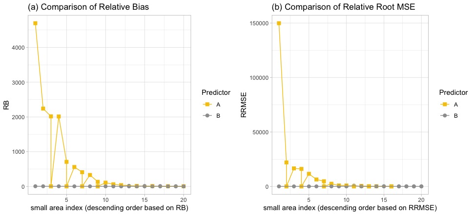
Figure 1: (a) Plot of RB for two predictors A and B. (b) Plot of RRMSE for two predictors A and B. We assume $m=20$ and $k=50\%$.

We consider nominal coverage $100(1-\alpha)\%=90\%$, $95\%$, and $99\%$. The results are given in Table 4. Overall, the bootstrap method outperforms the other three methods.

The coverage probabilities for bootstrap method are close to the nominal coverage, thus the intervals more accurately include the truth. Prediction intervals based on the direct method, estimated MSE, and jackknife are not reliable as they do not approximately follow the normal theory. Additionally, the latter two usually suffer from coverage problem because of the choice of MSE estimator and small values of $m$.

Table 4: Comparison of coverage probabilities and mean of the log lengths for the prediction intervals across all the methods. The results for the lengths are averaged over all the small areas. Additionally, we assume $k=50\%$ for all the cases.

Nominal	Small Areas	Direct	Estimated MSE	Jackknife	Bootstrap
Coverage	$m$
$90\%$	20	0.520	0.450	0.420	0.990
		(15.383)	(12.195)	(13.646)	(30.463)
	50	0.688	0.596	0.718	0.928
		(18.483)	(19.754)	(16.708)	(32.969)
$95\%$	20	0.560	0.450	0.420	1.000
		(15.561)	(12.374)	(13.824)	(37.314)
	50	0.696	0.596	0.764	0.948
		(18.662)	(19.932)	(16.887)	(36.755)
$99\%$	20	0.560	0.500	0.500	1.000
		(15.836)	(12.649)	(14.099)	(38.346)
	50	0.736	0.596	0.791	0.992
		(18.936)	(20.207)	(17.161)	(37.692)

Applications to Census Bureau’s Data Sets

In this Section, we describe the steps used to apply the preceding theory to census data sets. The first application is related to the Census of Governments, where we illustrate our methodology at the state level. The second application is related to the Small Area Income and Poverty Estimates (SAIPE) Program, where we illustrate our methodology at the county level.

Census of Governments

The purpose of the Census of Governments is providing periodic and comprehensive statistics about governments and governmental activities, and it covers all the states and local governments in the United States. Data are obtained on government organizations, finances, and employment and include location, type, and characteristics of local governments and officials; see https://www.census.gov/econ/overview/go0100.html for further information.

Since 1957 the United States Census Bureau collects information from governmental units for years ending in $2$ and $7$. Here, we utilize data from $2007$ and $2012$ with $49$ states of the Continental United States (excluding Hawaii and District of Columbia) as our small areas of interest.

We define the parameter of interest $\theta_{i}$ to be the mean number of full-time employees per government at state $i$ from the 2012 data set. We define the covariate to be the corresponding mean from the 2007 data set. To define the response $y_{i}$, we select sample of sizes $4000$ and $8000$ governmental units from the 2012 data set. Similarly, we construct the covariate $W_{i}$ from an independent sample of $40,000$ and $80,000$ governmental units selected from the 2007 data set.

The distributions of response and covariate are displayed in Figures S3.1 and S3.2 of the Supplementary Material for sample sizes $4000$ and $8000$. We observe skewed patterns in both the average number of full-time employees from 2007 and 2012 which motivates our proposed framework. Before a logarithmic transformation, both variables fail the normality assumption, and the normality assumption is more justified after the logarithmic transformation.

The measurement error variances $C_{i}$’s for the covariates are obtained from a Taylor series approximation because of the logarithmic transformation, and the formula of variance in simple random sampling without replacement is used per each state in the original scale. Additionally, we used Taylor series approximation for the $\psi_{i}$. We assume the sampling variances to be known throughout the estimation procedure. Based on our proposed framework, we find the empirical predictor $\tilde{\theta}_{i,B}$.

We construct prediction intervals based on three methods of “Direct”, “Jackknife”, and “Bootstrap”. The box-plots of prediction interval lengths are given in Figure 2. We observe that the distribution of lengths based on non-parametric bootstrap method has less variation in comparison with both direct and jackknife methods. Additionally, the descriptive statistics of lengths for $95\%$ prediction intervals are given in Table 5. We clearly observe more stable results for the descriptive statistics under the bootstrap method.

Table 5: Descriptive statistics for the log lengths of 95$\%$ prediction intervals from the Census of Governments. The results are computed using data from all the small areas.

Sample Size	Method	Minimum	$25\%$	Median	Mean	$75\%$	Maximum
4000	Bootstrap	4.320	4.350	4.360	4.370	4.380	4.410
	Direct	4.330	6.380	6.730	6.970	7.510	11.700
	Jackknife	-7.200	2.950	7.710	5.840	9.660	12.000
8000	Bootstrap	4.160	4.210	4.230	4.220	4.250	4.270
	Direct	5.370	6.420	7.000	7.150	7.780	10.000
	Jackknife	-15.600	-1.560	6.400	3.760	8.590	11.300

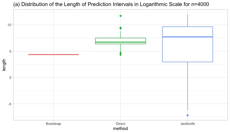
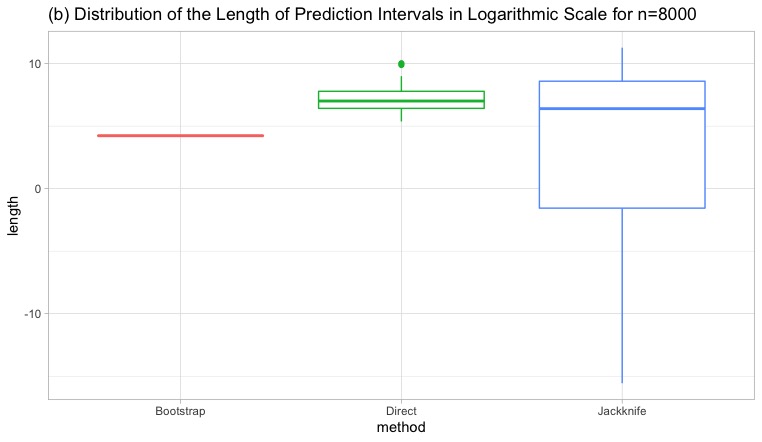
Figure 2: box-plots of prediction interval lengths with $1-\alpha=0.95$ based on three methods for the Census of Governments assuming (a) 4000 and (b) 8000 sample sizes.

Small Area Income and Poverty Estimates Program

The U.S. Census Bureau’s SAIPE program uses Fay and Herriot (1979) model to produce model-based estimates of income and poverty at the state and county levels for various age groups. Since 2005, they use the data from the American Community Survey (ACS) in the modeling. Prior to 2005, data from the Current Population Survey were used. The ACS is the largest U.S. household survey and it almost covers 3.5 million addresses per year.

Despite the large sample size of the ACS, the 1-year direct estimates of the number of related school-aged (5-17 year old) children in poverty are highly variable for many small counties. Thus, SAIPE program uses the Fay and Herriot (1979) model to borrow strength from covariates such as log number of food-stamp participants, log number of IRS child exemptions in households in poverty, log number of related children aged 5-17 in poverty from previous census, etc. to improve the direct estimate of the logarithm of the single-year ACS poverty counts as the dependent variable. For more information on the SAIPE program, see the SAIPE web page at https://www.census.gov/programs-surveys/saipe.html.

Recent research by Huang and Bell (2012) and Franco and Bell (2015) suggests that the most recent previous 5-year ACS estimates instead of outdated census results can be used as a covariate (see, Arima et al. (2017)). However, 5-year ACS estimates are subject to the sampling errors rather than the census results. Thus, it is appropriate to use Fay and Herriot (1979) where covariates are measured with errors and a log transformation is required. As a consequence, our proposed predictor is well-suited for this scenario.

Here, we assume the parameter of interest is the total population for whom poverty status is determined for the age of 5 to 17 years in 2018 at the county level. The covariate is the corresponding total of 5-year aggregated values; i.e. 2013–2017 at the county level. Additionally, we use the 2018 SNAP data set as a separate covariate which is measured without error.

We summarize these variables as follows:

• $y_{i}$: 1-year ACS (2018) estimates for $i=1,...,827$.

• $W_{i}$: Aggregated 5-year ACS (2013–2017) estimates, measured with errors, and

• $x_{i}$: 2018 SNAP data set measured without error as a separate covariate.

Unlike the 5-year aggregated ACS, the information for counties with population less than 65,000 are not publicly released for a single-year ACS. We successfully linked the same m=827 counties across the resources, and we only provide predictions for these publicly available counties. In Figure S3.3 (a) given in the Supplementary Material, we display the scatter plots of these counties.

We observe that both 5-year ACS and SNAP are highly correlated with the response variable $y$. The skewness in the original scales diminishes after a logarithmic transformation (see Figure S3.3 (b) in the Supplementary Material). To obtain the variance of estimates, we use the 90$\%$ margin of error given in the data set for both the covariate and the response variable. Afterwards, we use a Taylor series approximation to obtain the variance of the logarithm of estimates.

In this Section, we intend to study three small area models as follows:

• Measurement error model predictor: For this model, we assume the response variable is the 1-year ACS and the covariate is the 5-year ACS (measured with error). Because of skewed patterns in the data set, we need to use a logarithmic transformation. For this purpose, we use predictor B.

• Fay-Herriot model predictor: For this model, we assume the response variable is the 1-year ACS and the covariate is the SNAP information (measured without error). Because of skewed patterns in the data set, we again use a logarithmic transformation. For this purpose, we use predictor $\tilde{\theta}_{i,B}^{0}$, the so-called FHeblup afterwards.

• Direct Estimator: The results are solely based on the single-year ACS estimates.

In Figure 3, we compare the distribution of prediction interval lengths for all the counties based on non-parametric bootstrap, jackknife, direct, and FHeblup. We observe that the box-plot for the prediction interval lengths based on the non-parametric bootstrap method has a stable distribution.

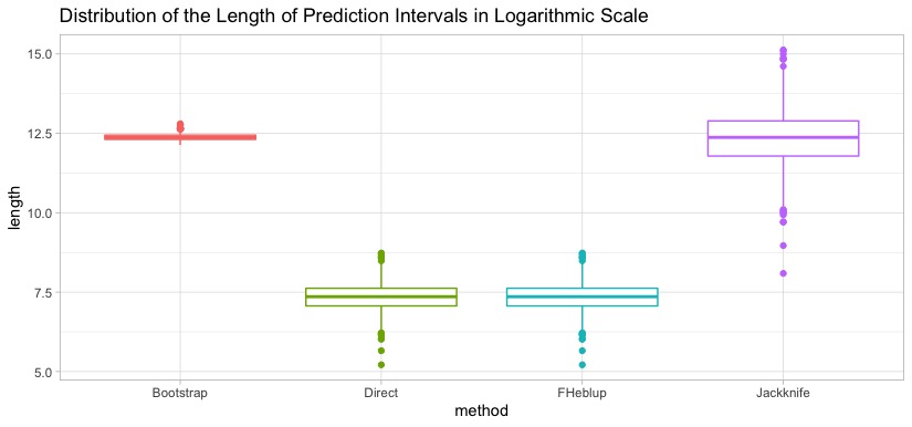
Figure 3: Box-plots of prediction interval lengths with $1-\alpha=0.95$ for the SAIPE data set. Note that the results are in the logarithmic scale.

Additionally, box-plots of direct and FHeblup are similar due to the close values of direct estimators and FHeblups (see Figure S3.4 in the Supplementary Material). This means the values of $\tilde{\theta}_{i,B}^{0}$ are close to $z_{i}$, which requires $\psi_{i}\approx 0$. This can be confirmed by the range of $\psi_{i}$, which is (6.579 e-07, 6.843 e-03). The values of mean, median, and standard deviation of the lengths for all the prediction intervals are given in Table 6.

Table 6: Mean, median, and standard deviation for the log lengths of 95$\%$ prediction intervals from the SAIPE data set. The results are computed using data from all the small areas.

Method	Median	Mean	Standard Deviation
Bootstrap	12.360	12.400	0.112
Direct	7.358	7.342	0.453
FHeblup	7.357	7.342	0.453
Jackknife	12.370	12.340	0.905

Discussion and Future Work

We propose a new predictor for the skewed response variable under Fay-Herriot model when the covariate is measured with error. Our set-up can be easily extended to the multivariate covariate case, and some of the steps in this regard are given in the Supplementary Material. While the proposed method is for area level model, it would be possible to consider an extension to unit level models, which is left to a future work.

This modeling framework can be of interest for government agencies and survey practitioners dealing with right skewed response variables and covariates that are measured with errors. Our proposed predictor is unbiased and can perform uniformly better than the direct estimator and the alternative predictor gien in the literature by Mosaferi et al. (2023). Further, we derive an approximation of the MSE of predictor, which does not perform well for constructing prediction intervals in terms of coverage. Thus, we develop nonparametric bootstrap prediction intervals.

Prediction intervals based on nonparametric bootstrap techniques are easy and allow a good coverage property. In particular, they can be more suitable for real applications as we use the available data sets for generating resamples. It might be of interest to investigate other resampling methods such as parametric bootstrap methods or extend the earlier works of log-MSPE by Jiang et al. (2018) to construct prediction intervals and make comparisons among them for our modeling framework.

Supplementary Material

The online Supplementary Material includes technical details, proofs of the theorems, and additional numerical results.

This supplementary material is structured as follows. Regularity conditions are given in Section S1. Further simulation and application results are given in Sections S2 and S3, respectively. Section S4 contains multivariate covariate setup. We provide proofs of theorems and some technical derivations in Sections S5 and S6.

S1  Regularity conditions

We give three regularity conditions as follows:

Condition 1. $\{(y_{i},W_{i},\psi_{i})\}$ is a sequence of independent and identically distributed random vectors, and there exist positive constants $\psi_{L}$ and $\psi_{U}$ such that $0<\psi_{L}\leq\inf_{1\leq i\leq m}\psi_{i}\leq\sup_{1\leq i\leq m}\psi_{i}\leq\psi_{U}<\infty$ for $i=1,...,m$.

Condition 2. $\bm{\omega}=(\beta_{0},\beta_{1},\sigma^{2}_{v})^{\prime}\in\Theta$ where $\Theta$ is a compact set such that $\Theta\subset(\mathbb{R},\mathbb{R},\mathbb{R}_{+})$ and $\hat{\bm{\omega}}\xrightarrow{P}\bm{\omega}$.

Condition 3. (i) $\tilde{U}(\bm{\omega})$ exists almost surely in probability and $E\{\tilde{U}(\bm{\omega})\}=0$. (ii) $\tilde{U}^{\prime}(\bm{\omega})$ is a continuous function where $E\{\tilde{U}^{\prime}(\bm{\omega})\}$ is uniformly bounded away from zero. (iii) $E\{|\tilde{U}(\bm{\omega})|^{4+\delta}\}$, $E\{|\tilde{U}^{\prime}(\bm{\omega})|^{4+\delta}\}$, and $E\{\sup_{c\in(-\epsilon,\epsilon)}|\tilde{U}^{\prime\prime}(\bm{\omega})|^{4+\delta}\}$ are uniformly bounded under some $\epsilon>0$ and $\delta>0$.

S2  Further simulation results

In this Section, we provide the empirical MSE of predictors as well as $\hat{R}_{1i}$ and $mse_{J}$ for multiple values of small areas related to the simulation Section of the paper. The results are listed in Table S2.1.

Table S2.1: Empirical MSE as well as $\hat{R}_{1i}$ and $mse_{J}$ of predictors averaged by the values of $C_{i}$ for all possible values of $k$. We assume $m\in\{20,50,100\}$, and the numerical values are in the logarithmic scale.

$k$	$C_{i}$	EMSE($y_{i}$)	EMSE($\tilde{\theta}_{i,\text{No-ME}}$)	EMSE($\tilde{\theta}_{i,A}$)	EMSE($\tilde{\theta}_{i,B}$)	$\hat{R}_{1i}(\tilde{\theta}_{i,B})$	$mse_{J}(\tilde{\theta}_{i,B})$
$m=20$
25	0	44.678	33.385	33.385	33.385	54.275	57.497
	2	48.742	37.031	50.733	38.925	90.202	80.191
50	0	48.514	38.684	38.684	38.684	63.755	63.852
	2	42.568	36.193	44.793	34.408	73.667	72.889
80	0	47.321	40.189	40.189	40.189	62.135	65.010
	2	43.966	37.164	46.019	35.167	79.058	78.690
100	2	45.600	38.923	47.445	37.089	81.210	78.617
$m=50$
25	0	48.779	37.851	37.851	37.851	66.433	68.337
	2	47.535	37.699	49.199	39.195	90.517	89.474
50	0	47.239	37.227	37.227	37.227	63.285	65.029
	2	50.841	41.380	52.488	42.141	96.313	94.237
80	0	49.722	40.308	40.308	40.308	71.310	74.125
	2	48.903	41.514	50.419	40.469	90.451	88.179
100	2	48.613	42.374	49.999	41.082	89.500	88.080
$m=100$
25	0	40.311	28.807	28.807	28.807	49.891	52.212
	2	49.897	38.359	51.599	40.349	92.106	89.288
50	0	46.091	35.481	35.481	35.481	62.508	64.791
	2	39.885	29.954	41.941	31.010	71.395	68.307
80	0	55.042	46.172	46.172	46.172	77.347	77.868
	2	39.988	33.310	41.700	32.434	72.332	71.142
100	2	42.977	36.106	44.535	35.132	78.235	77.868

S3  Further application results

In this Section, we provide three figures related to the application Section of the paper. Figures S3.1 and S3.2 depict the distributions of the Census of Governments based on 4000 and 8000 sample sizes. Figure S3.3 shows the scatter plots for the SAIPE data set. Figure S3.4 displays the box-plots of two predictors from the SAIPE data set.

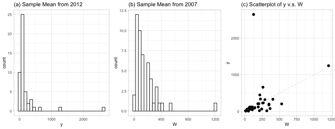
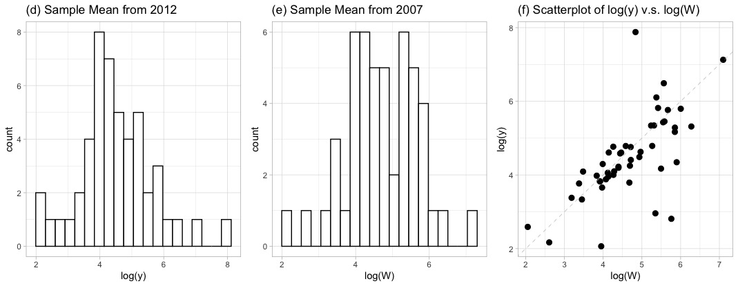
Figure S3.1: Histograms for the Census of Governments based on 4000 sample size. In both plots (a) and (b), the distributions of covariate and response are highly skewed to the right side. After transformations and in plots (d) and (e), we observe a stabilized distribution. Plots (c) and (f) display the regression relationship between the response variable and covariate before and after transformation.

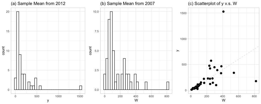
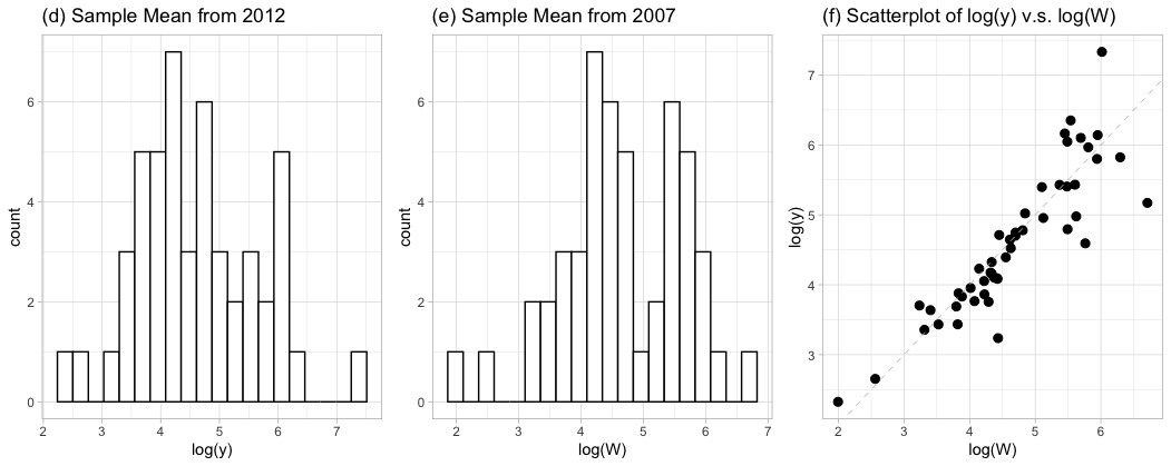
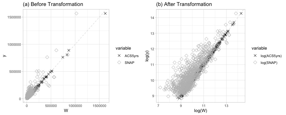
Figure S3.2: Histograms for the Census of Governments based on 8000 sample size. In both plots (a) and (b), the distributions of covariate and response are highly skewed to the right side. After transformations and in plots (d) and (e), we observe a stabilized distribution. Plots (c) and (f) display the regression relationship between the response variable and covariate before and after transformation.

Figure S3.3: Scatter plots of response variable versus covariates (a) before and (b) after transformations for the SAIPE data set.

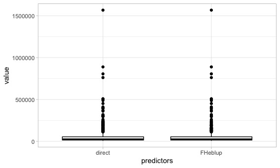
Figure S3.4: Box-plots of direct and FHeblup predictors for the SAIPE data set.

S4  Multivariate extension

In this Section, we give some details of formulation and forms of predictors A and B for multivariate covariate set-up. Let’s assume the following hierarchical set-up

$$z_{i}|\phi_{i} \sim N(\phi_{i},\psi_{i})$$

$$\phi_{i} \sim N(\beta_{0}+\bm{\beta}^{\prime}\bm{x}_{i},\sigma^{2}_{v})$$

$$\bm{W_{i}} \sim\textit{MVN}(\bm{x}_{i},\bm{C}_{i}),$$

where $\bm{\beta}^{\prime}=(\beta_{1},\beta_{2},...,\beta_{p})$, $\bm{x}_{i}=(x_{i1},x_{i2},...,x_{ip})^{\prime}$, $\bm{W}_{i}=(W_{i1},W_{i2},...,W_{ip})^{\prime}$, and $\bm{C}_{i}=\text{diag}(C_{i1},...,C_{ip})$.

The parameter of interest is $\theta_{i}=\exp(\beta_{0}+\bm{\beta}^{\prime}\bm{x}_{i}+v_{i})$. Following the same derivations given in the manuscript, predictor A can be defined as

$$\tilde{\theta}_{i,A}=\exp(\tilde{\gamma}_{i}z_{i}+(1-\tilde{\gamma}_{i})(\beta_{0}+\bm{\beta}^{\prime}\bm{W}_{i})+\tilde{\gamma}_{i}\psi_{i}/2),$$

where $\tilde{\gamma}_{i}=(\bm{\beta}^{\prime}\bm{C}_{i}\bm{\beta}+\sigma^{2}_{v})/S_{i}(\bm{\beta},\sigma^{2}_{v})$ and $S_{i}(\bm{\beta},\sigma^{2}_{v})=(\bm{\beta}^{\prime}\bm{C}_{i}\bm{\beta}+\sigma^{2}_{v}+\psi_{i})$. Predictor B can be defined as $\tilde{\theta}_{i,B}=\tilde{\theta}_{i,A}\exp(-\frac{1}{2}d_{i})$, where $d_{i}=2\psi_{i}\bm{\beta}^{\prime}\bm{C}_{i}\bm{\beta}/S_{i}(\bm{\beta},\sigma^{2}_{v})$. The vector of unknown parameters can be estimated along the same lines of the manuscript.

S5  Proofs of theorems

In this Section, we provide proofs of theorems.

Proof of Theorem 1:

$$E[\tilde{\theta}_{i,A}] =E[\exp(\tilde{\gamma}_{i}z_{i})]E[\exp\{(1-\tilde{\gamma}_{i})(\beta_{0}+\beta_{1}W_{i})\}]\exp(\tilde{\gamma}_{i}\psi_{i}/2)$$

$$=\exp[\tilde{\gamma}_{i}(\beta_{0}+\beta_{1}x_{i}+\frac{1}{2}\tilde{\gamma}_{i}^{2}(\sigma^{2}_{v}+\psi_{i}))]$$

$$\quad\times\exp[(1-\tilde{\gamma}_{i})(\beta_{0}+\beta_{1}x_{i}+\frac{1}{2}(1-\tilde{\gamma}_{i})^{2}(\beta_{1}^{2}C_{i}))]\exp(\tilde{\gamma}_{i}\psi_{i}/2)$$

$$=\exp[\beta_{0}+\beta_{1}x_{i}+\frac{1}{2}\{\tilde{\gamma}_{i}^{2}(\sigma^{2}_{v}+\psi_{i})+(1-\tilde{\gamma}_{i})^{2}(\beta_{1}^{2}C_{i})+\tilde{\gamma}_{i}\psi_{i}\}].$$ (S5.1)

Next, we simplify

$$\tilde{\gamma}_{i}^{2}(\sigma^{2}_{v}+\psi_{i})+(1-\tilde{\gamma}_{i})^{2}\beta_{1}^{2}C_{i}+\tilde{\gamma}_{i}\psi_{i}$$

$$\qquad=\tilde{\gamma}_{i}^{2}(\sigma^{2}_{v}+\psi_{i}+\beta_{1}^{2}C_{i})-2\tilde{\gamma}_{i}\beta_{1}^{2}C_{i}+\beta_{1}^{2}C_{i}+\tilde{\gamma}_{i}\psi_{i}$$

$$\qquad=S_{i}^{-1}(\beta_{1},\sigma^{2}_{v})(\beta_{1}^{2}C_{i}+\sigma^{2}_{v})^{2}-2\tilde{\gamma}_{i}\beta_{1}^{2}C_{i}+\beta_{1}^{2}C_{i}+\tilde{\gamma}_{i}\psi_{i}$$

$$\qquad=\tilde{\gamma}_{i}(\beta_{1}^{2}C_{i}+\sigma^{2}_{v})-2\tilde{\gamma}_{i}\beta_{1}^{2}C_{i}+\beta_{1}^{2}C_{i}+\tilde{\gamma}_{i}\psi_{i}$$

$$\qquad=\tilde{\gamma}_{i}(\sigma^{2}_{v}+\psi_{i})+(1-\tilde{\gamma}_{i})\beta_{1}^{2}C_{i}.$$ (S5.2)

The result follows from (S5  Proofs of theorems) and (S5  Proofs of theorems).

Proof of Theorem 2: We use the equations from the expressions (4) of the manuscript to find the matrix $I_{\bm{\omega}}$ as follows

$$I_{\bm{\omega}}=\begin{bmatrix}var(\tilde{U}_{1}(\bm{\omega}))&cov(\tilde{U}_{1}(\bm{\omega}),\tilde{U}_{2}(\bm{\omega}))&cov(\tilde{U}_{1}(\bm{\omega}),\tilde{U}_{3}(\bm{\omega}))\\ cov(\tilde{U}_{1}(\bm{\omega}),\tilde{U}_{2}(\bm{\omega}))&var(\tilde{U}_{2}(\bm{\omega}))&cov(\tilde{U}_{2}(\bm{\omega}),\tilde{U}_{3}(\bm{\omega}))\\ cov(\tilde{U}_{1}(\bm{\omega}),\tilde{U}_{3}(\bm{\omega}))&cov(\tilde{U}_{2}(\bm{\omega}),\tilde{U}_{3}(\bm{\omega}))&var(\tilde{U}_{3}(\bm{\omega}))\end{bmatrix}.$$

The elements of the matrix are as follows

$$var(\tilde{U}_{1}(\bm{\omega})) =\sum_{i=1}^{m}S_{i}^{-1}(\beta_{1},\sigma^{2}_{v}),$$

$$cov(\tilde{U}_{1}(\bm{\omega}),\tilde{U}_{2}(\bm{\omega})) =\sum_{i=1}^{m}S_{i}^{-2}(\beta_{1},\sigma^{2}_{v})cov[W_{i}\tau_{i}(\beta_{0},\beta_{1}),\tau_{i}(\beta_{0},\beta_{1})]$$

$$=\sum_{i=1}^{m}S_{i}^{-2}(\beta_{1},\sigma^{2}_{v})E[(W_{i}-x_{i}+x_{i})\tau_{i}^{2}(\beta_{0},\beta_{1})]=\sum_{i=1}^{m}S_{i}^{-1}(\beta_{1},\sigma^{2}_{v})x_{i},$$

$$cov(\tilde{U}_{1}(\bm{\omega}),\tilde{U}_{3}(\bm{\omega})) =0,$$

$$var(\tilde{U}_{2}(\bm{\omega})) =\sum_{i=1}^{m}S_{i}^{-2}(\beta_{1},\sigma^{2}_{v})var[W_{i}\tau_{i}(\beta_{0},\beta_{1})]+\beta_{1}^{2}\sum_{i=1}^{m}S_{i}^{-4}(\beta_{1},\sigma^{2}_{v})C_{i}^{2}\,var[\tau_{i}^{2}(\beta_{0},\beta_{1})]$$

$$\quad+2\beta_{1}\sum_{i=1}^{m}S_{i}^{-3}(\beta_{1},\sigma^{2}_{v})C_{i}cov[W_{i}\tau_{i}(\beta_{0},\beta_{1}),\tau_{i}^{2}(\beta_{0},\beta_{1})].$$

Note that we have

• $var[W_{i}\tau_{i}(\beta_{0},\beta_{1})]=(x_{i}^{2}+C_{i})S_{i}(\beta_{1},\sigma^{2}_{v})+\beta_{1}^{2}C_{i}^{2}$,

• $var[\tau_{i}^{2}(\beta_{0},\beta_{1})]=2S_{i}^{2}(\beta_{1},\sigma^{2}_{v})$, and

• $cov[W_{i}\tau_{i}(\beta_{0},\beta_{1}),\tau_{i}^{2}(\beta_{0},\beta_{1})]=-2\beta_{1}C_{i}S_{i}(\beta_{1},\sigma^{2}_{v})$.

Therefore,

$$var(\tilde{U}_{2}(\bm{\omega})) =\sum_{i=1}^{m}S_{i}^{-2}(\beta_{1},\sigma^{2}_{v})(\sigma^{2}_{v}+\psi_{i})C_{i}+\sum_{i=1}^{m}S_{i}^{-1}(\beta_{1},\sigma^{2}_{v})x_{i}^{2}=\sum_{i=1}^{m}S_{i}^{-1}(\beta_{1},\sigma^{2}_{v})(x_{i}^{2}+\tilde{\sigma}^{2}_{ci}),$$

$$cov(\tilde{U}_{2}(\bm{\omega}),\tilde{U}_{3}(\bm{\omega})) =\frac{1}{2}cov[\sum_{i=1}^{m}S_{i}^{-1}(\beta_{1},\sigma^{2}_{v})W_{i}\tau_{i}(\beta_{0},\beta_{1})+\beta_{1}\sum_{i=1}^{m}S_{i}^{-2}(\beta_{1},\sigma^{2}_{v})C_{i}\tau_{i}^{2}(\beta_{0},\beta_{1}),$$

$$\sum_{i=1}^{m}S_{i}^{-1}(\beta_{1},\sigma^{2}_{v})\tau_{i}^{2}(\beta_{0},\beta_{1})]$$

$$=\frac{1}{2}\sum_{i=1}^{m}S_{i}^{-3}(\beta_{1},\sigma^{2}_{v})cov[W_{i}\tau_{i}(\beta_{0},\beta_{1}),\tau_{i}^{2}(\beta_{0},\beta_{1})]$$

$$\quad+\frac{1}{2}\beta_{1}\sum_{i=1}^{m}S_{i}^{-4}(\beta_{1},\sigma^{2}_{v})C_{i}var[\tau_{i}^{2}(\beta_{0},\beta_{1})]=-\beta_{1}\sum_{i=1}^{m}S_{i}^{-2}(\beta_{1},\sigma^{2}_{v})C_{i}$$

$$\quad+\beta_{1}\sum_{i=1}^{m}S_{i}^{-2}(\beta_{1},\sigma^{2}_{v})C_{i}=0,$$

$$var(\tilde{U}_{3}(\bm{\omega})) =\frac{1}{4}\sum_{i=1}^{m}S_{i}^{-4}(\beta_{1},\sigma^{2}_{v})var[\tau_{i}^{2}(\beta_{0},\beta_{1})]=\frac{1}{2}\sum_{i=1}^{m}S_{i}^{-2}(\beta_{1},\sigma^{2}_{v}).$$

As a final result, we get

$$I_{\bm{\omega}}=\begin{bmatrix}\sum_{i=1}^{m}S_{i}^{-1}(\beta_{1},\sigma^{2}_{v})&\sum_{i=1}^{m}S_{i}^{-1}(\beta_{1},\sigma^{2}_{v})x_{i}&0\\ \sum_{i=1}^{m}S_{i}^{-1}(\beta_{1},\sigma^{2}_{v})x_{i}&\sum_{i=1}^{m}S_{i}^{-1}(\beta_{1},\sigma^{2}_{v})(x_{i}^{2}+\tilde{\sigma}^{2}_{ci})&0\\ 0&0&\frac{1}{2}\sum_{i=1}^{m}S_{i}^{-2}(\beta_{1},\sigma^{2}_{v})\end{bmatrix}.$$

S6  Details of derivations for $\hat{R}_{1i}$

Recall that $R_{1i}:=M_{1i}(\bm{\omega})M_{2i}(\bm{\omega})$. In order to estimate $R_{1i}$, one can define

$$E[M_{1i}(\hat{\bm{\omega}})M_{2i}(\hat{\bm{\omega}})-M_{1i}(\bm{\omega})M_{2i}(\bm{\omega})]^{2}:=E[\{M_{1i}(\hat{\bm{\omega}})-M_{1i}(\bm{\omega})\}\{M_{2i}(\hat{\bm{\omega}})-M_{2i}(\bm{\omega})\}$$

$$\qquad+M_{2i}(\bm{\omega})(M_{1i}(\hat{\bm{\omega}})-M_{1i}(\bm{\omega}))+M_{1i}(\bm{\omega})(M_{2i}(\hat{\bm{\omega}})-M_{2i}(\bm{\omega}))]^{2}$$

$$\quad=E[\{M_{1i}(\hat{\bm{\omega}})-M_{1i}(\bm{\omega})\}^{2}\{M_{2i}(\hat{\bm{\omega}})-M_{2i}(\bm{\omega})\}^{2}]$$

$$\qquad+M_{2i}^{2}(\bm{\omega})E[M_{1i}(\hat{\bm{\omega}})-M_{1i}(\bm{\omega})]^{2}+M_{1i}^{2}(\bm{\omega})E[M_{2i}(\hat{\bm{\omega}})-M_{2i}(\bm{\omega})]^{2}$$

$$\qquad+2E[(M_{1i}(\hat{\bm{\omega}})-M_{1i}(\bm{\omega}))^{2}(M_{2i}(\hat{\bm{\omega}})-M_{2i}(\bm{\omega}))]M_{2i}(\bm{\omega})$$

$$\qquad+2E[(M_{1i}(\hat{\bm{\omega}})-M_{1i}(\bm{\omega}))(M_{2i}(\hat{\bm{\omega}})-M_{2i}(\bm{\omega}))^{2}]M_{1i}(\bm{\omega})$$

$$\qquad+2M_{1i}(\bm{\omega})M_{2i}(\bm{\omega})E[(M_{1i}(\hat{\bm{\omega}})-M_{1i}(\bm{\omega}))(M_{2i}(\hat{\bm{\omega}})-M_{2i}(\bm{\omega}))].$$ (S6.1)

Application of the Cauchy-Schwarz inequality yields

(i) $$E[\{M_{1i}(\hat{\bm{\omega}})-M_{1i}(\bm{\omega})\}^{2}\{M_{2i}(\hat{\bm{\omega}})-M_{2i}(\bm{\omega})\}^{2}]$$

$$\quad\leq E^{1/2}[M_{1i}(\hat{\bm{\omega}})-M_{1i}(\bm{\omega})]^{4}E^{1/2}[M_{2i}(\hat{\bm{\omega}})-M_{2i}(\bm{\omega})]^{4}=O(1)O(m^{-1})=O(m^{-1}),$$

(ii) $$E[\{M_{1i}(\hat{\bm{\omega}})-M_{1i}(\bm{\omega})\}^{2}\{M_{2i}(\hat{\bm{\omega}})-M_{2i}(\bm{\omega})\}]$$

$$\quad\leq E^{1/2}[M_{1i}(\hat{\bm{\omega}})-M_{1i}(\bm{\omega})]^{4}E^{1/2}[M_{2i}(\hat{\bm{\omega}})-M_{2i}(\bm{\omega})]^{2}=O(1)O(m^{-1/2})=O(m^{-1/2}),$$

(iii) $$E[\{M_{1i}(\hat{\bm{\omega}})-M_{1i}(\bm{\omega})\}\{M_{2i}(\hat{\bm{\omega}})-M_{2i}(\bm{\omega})\}^{2}]$$

$$\quad\leq E^{1/2}[M_{1i}(\hat{\bm{\omega}})-M_{1i}(\bm{\omega})]^{2}E^{1/2}[M_{2i}(\hat{\bm{\omega}})-M_{2i}(\bm{\omega})]^{4}=O(1)O(m^{-1})=O(m^{-1}),$$

(iv) $$E[M_{2i}(\hat{\bm{\omega}})-M_{2i}(\bm{\omega})]^{2}=O(m^{-1}),\quad\text{and}$$

(v) $$E[\{M_{1i}(\hat{\bm{\omega}})-M_{1i}(\bm{\omega})\}\{M_{2i}(\hat{\bm{\omega}})-M_{2i}(\bm{\omega})\}]$$

$$\quad\leq E^{1/2}[M_{1i}(\hat{\bm{\omega}})-M_{1i}(\bm{\omega})]^{2}E^{1/2}[M_{2i}(\hat{\bm{\omega}})-M_{2i}(\bm{\omega})]^{2}=O(1)O(m^{-1/2})=O(m^{-1/2}).$$

Thus, we conclude that only the term $M^{2}_{2i}(\bm{\omega})E[M_{1i}(\hat{\bm{\omega}})-M_{1i}(\bm{\omega})]^{2}$ from expression (S6  Details of derivations for $\hat{R}_{1i}$) needs to be estimated. Therefore, the estimator of $R_{1i}$ is the expression of $\hat{R}_{1i}$ given in the manuscript.

References

• Arima et al. (2017) Arima, S., Bell, W., Datta, G. S., Franco, C. and Liseo, B. (2017) Multivariate Fay–Herriot Bayesian estimation of small area means under functional measurement error Journal of the Royal Statistical Society: Series A 180, 1191–1209.
• Berg and Chandra (2014) Berg, E. and Chandra, H. (2014) Small area prediction for a unit–level lognormal model Computational Statistics & Data Analysis 78, 159–175.
• Butar and Lahiri (2003) Butar, F. B. and Lahiri, P. (2003) On measures of uncertainty of empirical Bayes small-area estimators Journal of Statistical Planning and Inference 112, 63–76.
• Carter and Rolph (1974) Carter, G. M. and Rolph, J. E. (1974) Empirical Bayes methods applied to estimating fire alarm probabilities Journal of the American Statistical Association 69, 880–885.
• Efron and Morris (1975) Efron, B. and Morris, C. (1975) Data analysis using Stein’s estimator and its generalizations Journal of the American Statistical Association 70, 311–319.
• Fay and Herriot (1979) Fay, R. E. and Herriot, R. A. (1979) Estimates of income for small places: an application of James–Stein procedures to census data Journal of the American Statistical Association 74, 269–277.
• Franco and Bell (2015) Franco, C. and Bell, W. R. (2015) Borrowing information over time in binomial/logit normal models for small area estimation Statistics in Transition new series 16, 563–584.
• Ghosh and Rao (1994) Ghosh, M. and Rao, J. N. K. (1994) Small area estimation: an appraisal Statistical Science 9, 55–76.
• Hall (2013) Hall, P. (2013) The Bootstrap and Edgeworth Expansion Springer Science & Business Media.
• Huang and Bell (2012) Huang, E. T. and Bell, W. R. (2012) An empirical study on using previous American community survey data versus census 2000 data in SAIPE models for poverty estimates Statistics 4, 1–35.
• Jiang et al. (2018) Jiang, J., Lahiri, P. and Nguyen, T. (2018) A unified Monte-Carlo jackknife for small area estimation after model selection Annals of Mathematical Sciences and Applications 3, 405–438.
• Jiang et al. (2002) Jiang, J., Lahiri, P. and Wan, S. M. (2002) A unified jackknife theory for empirical best prediction with M-estimation The Annals of Statistics 30, 1782–1810.
• Lahiri (2003) Lahiri, S. (2003) Resampling Methods for Dependent Data Springer Science & Business Media.
• Molina and Martín (2018) Molina, I. and Martín, N. (2018) Empirical best prediction under a nested error model with log transformation The Annals of Statistics 46, 1961–1993.
• Mosaferi et al. (2023) Mosaferi, S., Ghosh, M. and Steorts, R. C. (2023) Transformed Fay–Herriot model with measurement error in covariates Communications in Statistics - Simulation and Computation 52, 2257–2274.
• Pfefferman (2013) Pfefferman, D. (2013) New important developments in small area estimation Statistical Science 28, 40–68.
• Prasad and Rao (1990) Prasad, N. G. N. and Rao, J. N. K. (1990) The estimation of the mean squared error of small–area estimators Journal of the American Statistical Association 85, 163–171.
• Rao and Molina (2015) Rao, J. N. K. and Molina, I. (2015) Small Area Estimation Wiley Series in Survey Sampling.
• Slud and Maiti (2006) Slud, E. V. and Maiti, T. (2006) Mean-squared error estimation in transformed Fay–Herriot models Journal of the Royal Statistical Society: Series B (Statistical Methodology) 68, 239–257.
• van der Vaart (2000) van der Vaart, A. W. (2000) Asymptotic Statistics vol. 3 Cambridge university press.
• Ybarra and Lohr (2008) Ybarra, L. M. and Lohr, S. L. (2008) Small area estimation when auxiliary information is measured with error Biometrika 95, 919–931.
SUPPLEMENTARY MATERIAL FOR “AN UNBIASED PREDICTOR FOR SKEWED RESPONSE VARIABLE WITH MEASUREMENT ERROR IN COVARIATE”
Sepideh Mosaferi, Malay Ghosh, and Shonosuke Sugasawa
University of Massachusetts Amherst, University of Florida
and Keio University