Optimal Dorfman Group Testing For Symmetric Distributions

Abstract

We study Dorfman’s classical group testing protocol in a novel setting where individual specimen statuses are modeled as exchangeable random variables. We are motivated by infectious disease screening. In that case, specimens which arrive together for testing often originate from the same community and so their statuses may exhibit positive correlation. Dorfman’s protocol screens a population of $n$ specimens for a binary trait by partitioning it into nonoverlapping groups, testing these, and only individually retesting the specimens of each positive group. The partition is chosen to minimize the expected number of tests under a probabilistic model of specimen statuses. We relax the typical assumption that these are independent and indentically distributed and instead model them as exchangeable random variables. In this case, their joint distribution is symmetric in the sense that it is invariant under permutations. We give a characterization of such distributions in terms of a function $q$ where $q(h)$ is the marginal probability that any group of size $h$ tests negative. We use this interpretable representation to show that the set partitioning problem arising in Dorfman’s protocol can be reduced to an integer partitioning problem and efficiently solved. We apply these tools to an empirical dataset from the COVID-19 pandemic. The methodology helps explain the unexpectedly high empirical efficiency reported by the original investigators.

60G09, 62E10, 62H05, 62P10, 90-08, 90C39, 90C90

1 Introduction

Group testing is widely used to conserve resources while performing large-scale disease screening. Logistical considerations often lead to the use of Dorfman’s simple two-stage adaptive procedure in practice. This protocol is usually based on probabilistic analyses of disease prevalence arising from models of specimen statuses as mutually independent random variables. In this paper, we generalize and study the case in which the statuses are modeled as exchangeable, but not necessarily independent, random variables.

Given a population of $n$ specimens to screen for a binary trait, the group testing framework allows for several specimens to be pooled and tested together as a group. The group tests positive if any of its individual specimens is positive. The group tests negative if, and only if, all of its specimens are negative. Numerous protocols using this testing capability have been proposed, of which Dorfman’s two-stage adaptive procedure is the earliest, simplest, and most widely used. In this protocol, the population is partitioned into nonoverlapping groups and these are tested in the first stage. If a group of size $h>1$ tests negative, each of its $h$ specimens is immediately determined negative and $h-1$ tests are saved. If a group tests positive, each of its specimens is retested individually in the second stage and determined according to the outcome of its individual test. The key question is how to partition the specimens.

Since tests are saved only when a group tests negative and these group test outcomes depend on the distribution and prevalence of positive specimens, a standard approach specifies a probabilistic model of specimen statuses and finds a partition to minimize the expected number of tests used. In general, both specifying the model and finding the partition are difficult. The first requires a parameterization, and the second a computation, which grows exponentially in the number of specimens to be tested. Historically, this complexity has been avoided via simple probabilistic models arising from a strong assumption of independence.

It is desirable from both a theoretical and practical point of view to alleviate the independence assumption. From a theoretical point of view, it is interesting to consider how one might efficiently find partitions for more complicated distributions. From a practical point of view, it is natural to suppose that the statuses of specimens arriving together for testing may be correlated because they originate from the same family, living place, or workplace and the disease is contagious. Indeed, a recent large-scale study cited this phenomenon when explaining the failure of current theoretical tools to predict observed empirical test savings [21]. It is a pleasant surprise, therefore, that one can model specimen statuses as exchangeable while maintaining interpretability of the probabilistic model and tractability of the computation.

1.1 Contributions

When individual statuses are modeled as exchangeable random variables their joint distribution is symmetric in the sense that it is invariant under permutations of its arguments. Our first contribution is to characterize such a symmetric distribution $p$ in terms of a function $q$, where $q(h)$ is the probability that a group of size $h$ tests negative. The representation $q$ is key to finding a partition to minimize the expected number of tests.

Our second contribution is to use this characterization, along with a natural reduction of additive and symmetric set partitioning problems to additive integer partitioning problems, to show how to efficiently compute optimal partitions for exchangeable statuses. In contrast to additive set partitioning problems, additive integer partitioning problems are tractable and several efficient algorithms are known for their solution. For details, see Section 4.

Lastly, we apply these tools to an empirical dataset from the COVID-19 pandemic. The data we use indicate empirical efficiency exceeding that predicted by the classical theory, which models statuses as independent and identically distributed. Our tools partially explain this empirical efficiency and also indicate a different and more efficient partition than that used by the original investigators. We make our numerical implementation available [122].

In summary, we study Dorfman’s two-stage adaptive group testing procedure for the case of exchangeable specimen statuses. Our three contributions are:

1. a characterization of symmetric distributions over binary outcomes

2. a method to efficiently find optimal testing partitions under such distributions

3. a numerical experiment applying these tools to an empirical COVID-19 dataset

Outline

In the following two subsections we give further background on related work and introduce our notation. In Section 2, we formalize Dorfman’s two-stage adaptive group testing protocol. In Section 3, we discuss and characterize symmetric distributions. In Section 4, we study the structure of symmetric and additive set partitioning problems and present tools for their solution. In Section 5, we numerically apply these tools to a COVID-19 dataset. We briefly conclude in Section 6 and list some directions for future work.

1.2 Background

We provide background on group testing, probabilistic symmetries and partitioning problems. Each is a highly developed field with an extensive literature.

1.2.1 Group testing

In 1943, Dorfman initiated the study of group testing, also called pooled testing, by proposing his original methodology for disease screening [55]. The field has grown considerably since. Today, it can be distinguished along several axes. We briefly characterize the setting of this paper before further outlining these areas.

Our setting

We study Dorfman’s two-stage, adaptive procedure in the probabilistic, finite-population setting with binary specimen statuses and binary, noiseless, unconstrained tests. The central novelty is in modeling the specimen statuses as exchangeable random variables. We are aware of only one other article studying restricted forms of exchangeability [126]. We also emphasize that we use the term symmetric, see Section 3, to describe the joint distribution of the statuses and not, as others have done [164, 56], to describe the testing model.

The key prior work for situating our contribution is Dorfman’s original article [55] and Hwang’s follow-up [90]. Both considered Dorfman’s adaptive two-stage procedure in a probabilistic setting, with noiseless binary test results. Hwang moved from Dorfman’s infinite population setting to a finite population setting and generalized Dorfman’s probabilistic model to allow for specimen-specific positive status probabilities. Our work generalizes Dorfman’s in a similar but parallel way. Rather than dropping the identically distributed assumption as Hwang does, we drop the independence assumption. We visualize this in Figure 1.

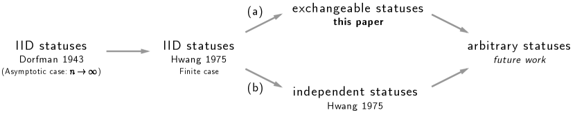
Figure 1: Assumptions for Dorfman’s two-stage adaptive group testing procedure with noiseless binary test results. (a) drops the independence assumption whereas (b) drops the identically distributed assumption.

Areas of group testing

Although a comprehensive survey of group testing is beyond the scope of this paper, we highlight some of the variety within the field.

A) Specimen status models, side information, and objective. A natural first distinction in group testing is between the probabilistic and combinatorial approach. This paper considers probabilistic group testing. Here, one specifies a probabilistic model of specimen statuses and performs testing to minimize some criterion usually related to expected efficiency. In the alternative combinatorial approach, one specifies information about the number of positive specimens and performs testing to minimize a worst-case criterion usually related to the maximum number of tests required. Hence a worst-case, or minimax [56], analysis replaces an average-case analysis. For examples of combinatorial group testing, starting with Li in 1962 [127], see [88, 111, 37, 38, 75, 63]. Hereafter we assume the probabilistic setting.

Within probabilistic group testing, a first further subdivision involves the related aspects of model choice and side information. For example, Dorfman [55] models binary specimen statuses as IID and assumes only knowledge of the prevalence, i.e. the probability that any given specimen is positive. Historically, several authors have followed his approach [168, 162, 174, 67, 180, 80, 164, 78, 154, 172], including two influential textbooks containing the so-called blood testing problem as exercises [66, 182]. This simple probabilistic model has been called the IID model [7], binomial model [150, 39], B-model [160], or binomial [119] or homogeneous population [10]. Some authors use the term binomial group testing [160, 89].

Many other probabilistic models have been considered besides the binomial. In 1968, Sobel considered a setting in which $d$ positive specimens are distributed uniformly throughout the population [160]. This has been called the hypergeometric model [159, 160, 98], H-model [160], or combinatorial prior [7]. The term generalized hypergeometric model [93] has been used when only an upper bound on $d$ is assumed, whereas the term truncated binomial model [94, 96] has been used if an upper bound is known for the binomial model. In 1973, Nebenzahl and Sobel [143] considered group testing for a population composed of several separate binomial populations with different prevalences. As mentioned above, Hwang [90] further generalized this direction by modeling specimens as independent but nonidentical binary random variables. This is called the generalized binomial model [90], prior defectivity model [7], nonidentical model [128, 112, 53], or heterogeneous population [58, 10, 31].

In this style, we might use the term exchangeable model or symmetric model to describe the exchangeable populations we consider herein. The information assumed is the $n$ parameters of the symmetric distribution. On one hand, the binomial, truncated binomial, hypergeometric, and generalized hypergeometric models are symmetric. On the other, the generalized binomial model is not symmetric. Previously, the so-called mean model [96] has been studied as a generalization of all of these. It assumes only the mean number of positives. Later on, we discuss other more recent models allowing correlation between specimen statuses.

Within probabilistic group testing, a second further subdivision relates to parameter uncertainty and the choice of objective. Starting with Sobel and Groll in 1959 [162], several authors handle uncertainty in model parameters [163, 120, 39, 107]. In this setting, the objective of estimation may replace that of efficiency [161, 39]. Elsewhere, other objectives such as information gain [2] and risk-based metrics [10] have been considered. See [85] for further discussion of different objectives. In the sequel, we assume full knowledge of model parameters and focus on the objective of efficiency as measured by the expected number of tests used.

B) Testing models, feasibility, and noise. A second distinction relates to the group testing capability. Dorfman [55] considers unconstrained, noiseless, binary individual and group tests. This is the setting we consider. The terms reliable [56] for noiseless and disjunctive [24] for binary group outcomes are also used. We mention alternative testing models for binary specimen statuses below. Historically, other testing models also arise naturally from nonbinary specimen status models, as for example the trinomial model [117] and multinomial model [118].

Toward more informative tests, we mention three examples. First, Sobel [160] considered quantitative group testing [7] in which group tests reveal the number of positive specimens. Sobel used the term H-type model, in contrast with the term B-type model for the usual binary result setting. As indicated earlier, he used analogous language for the specimen model. Other terms include linear model or adder channel model [7]. For variants on this theme, see [139, 61, 179]. Second, Pfeifer and Enis [150] considered group tests that reveal the sum or mean of individual test results. Although the distinction involves tests and not statuses, they use the term modified binomial model or M-model. For examples of fully continuous test results, see [181, 177]. Third, Sobel and coauthors [164] considered symmetric group testing [56] in which there are three group test outcomes: all positive, all negative, and mixed. We reiterate that symmetric here describes the test model and not the status model.

In the opposite direction, several authors weaken the group test capability. Toward less informative models, we mention Hwang [91] and Farach et al. [65] who consider dilution effects and so-called inhibitor specimens, respectively. For details and other examples, see the survey [7] and the book [56]. Similarly, application areas often motivate various forms of constrained group testing [7]. Two natural and classic examples limit the size of a group test [90] or the divisibility of a specimen [162]. Recently, these have been studied under the heading sparse group testing [69, 70, 103, 105]. For a second example, in graph-constrained group testing the tests must correspond to paths in a given graph [82, 109, 41, 158, 158, 165]. The methodology we give below readily handles limits on group size. We consider no additional constraints.

Starting with Graff and Roeloffs in 1972 [78], authors regularly study probabilistic models of noisy, or unreliable, tests [114, 107, 4]. Noisy tests motivate studying nonexact, or partial, recovery as opposed to exact recovery [7]. In the sequel, we only consider reliable tests.

C) Algorithms and analysis. A third distinction in group testing involves the algorithms and analysis considered. The algorithmic distinction is largely captured by a division into adaptive and nonadaptive procedures. The analytical distinction is largely captured by a division into finite population and infinite population, or asymptotic, analysis.

The terms adaptive, sequential and multistage describe procedures with multiple rounds, cycles, or stages of testing [56]. The tests of later rounds may depend on, and so adapt to, the results of earlier ones. Each round may involve one test or several. The literature is replete with adaptive algorithms [125, 74, 90, 112, 33, 53]. The further modifiers nested [92, 134] and hierarchical [114, 170, 106] indicate that groups tested in later stages are subsets of groups already tested. For example, a classic multistage nested approach is Sobel and Groll’s original binary splitting or halving [162]. For a modern discussion and further examples, see [7, 56].

Alternatively, various applications motivate nonadaptive, or single-stage, algorithms in which all group tests must be specified in advance [100, 20, 36, 40, 57, 41, 7]. Although it is sometimes natural in this case to discuss the two stages of testing and decoding [7], we use the term two-stage exclusively in its usual sense [24, 47, 141] of two rounds of testing.

Dorfman’s [55] particular two-stage, adaptive strategy splits the population into nonoverlapping groups of a fixed size, tests these, and individually retests the specimens of positive groups. The strategy has been called the Dorfman procedure [78, 90, 150, 96], Dorfman-type group testing [150], Dorfman screening [137, 152], Dorfman testing [10], and single pooling [33]. Some authors use the terms conservative [6] or trivial [47] when the second round of a two-stage procedure only involves individual retests. These terms are usually employed, however, when confirmatory [65] tests are used to verify suspected positives indicated by a first round of overlapping tests. This occurs, for example, in array testing [151, 138].

Dorfman [55] considers the setting in which the population size tends to infinity. This asymptotic regime remains popular, especially in the information theory community [7]. On the other hand, starting with Sobel and Groll in 1959 [162], many authors consider finite populations [118, 74, 90] or both settings [143, 164, 150]. We consider herein the finite-population setting in which Dorfman’s procedure is generalized slightly to allow for groups of different sizes. Hence one seeks a partition of the population. See Section 2 for details.

Applications beyond disease screening

In his original article, Dorfman [55] speculated on the utility of group testing outside of medical testing. In particular, he mentioned manufacturing quality control. Sobel and Groll’s influential 1959 article [162] gave further examples. See also the book [106]. Since then, researchers have applied group testing techniques in such diverse settings as wireless communications [83, 25, 183, 131, 103, 104, 102, 105, 42], genetics [79, 34, 133, 101], machine learning [173, 186, 135], signal processing [73, 43] and data stream analysis [45, 60]. The survey [7] and the book [56] contain additional applications and references.

Application to COVID-19 pandemic

The COVID-19 pandemic created a surge of interest in group testing for disease screening [136, 59, 17]. We make four observations here. First, pooling was feasible. Standard technology detects SARS-CoV-2 virus in pools of up to 32 specimens [184, 178]. Second, pooling was widely and successfully used in practical settings [86, 184, 130, 23, 21] and encouraged by authorities [142, 147, 16, 169, 1, 175, 46]. Third, practitioners often preferred Dorfman’s procedure for reasons, among simplicity, that we detail below [23, 21]. Other sophisticated approaches were, however, proposed [140, 72, 87]. Finally, the classical independence theory failed to explain empirical findings in large-scale asymptomatic screening [21, 44]. We discuss this and work aiming to remediate it below.

Benefits of Dorfman’s procedure

There are good reasons to prefer Dorfman’s protocol beyond its simplicity, historical precedence and modern importance. First, it divides each specimen into only two aliquots. This feature is relevant when the testing process is destructive or dilutive, as is usually the case in disease screening or any biological specimen testing. Second, it is parallel. Within both stages, all indicated tests can be performed at the same time. Consequently, the latency is predictable and bounded. The test efficiency gains of more sophisticated procedures, e.g. Sterrett’s [168] or binary splitting [162], are often offset by latency considerations. Third, it has easy to compute pool sizes and interpretable results. The methodology we develop for exchangeable populations also enjoys these features.

Group testing with specimen status correlation

The pandemic created a surge of interest in studying group testing under models motivated by infectious disease screening. These often include correlation between statuses, a feature largely absent from the classical literature. Furthermore, these models involve various forms and degrees of side information. While it is reasonable to suppose that such side information can help efficiency, is is natural to be interested in methodology independent of it. Modeling exchangeability requires no additional knowledge of contact tracing, interaction networks, or community structure.

Although Hwang mentions correlated statuses in his 1984 discussion of the mean model [96], Lendle et al.’s [126] 2012 article appears to be the first to study correlated specimen statuses in earnest. They investigate a restricted form of exchangeability and show that efficiency gains can result from pooling within clusters of positively correlated specimens.

We highlight three more recent directions here. First, Lin et al. [129] study the Dorfman procedure under a correlated arrival process of contiguous groups from different IID populations. They find higher efficiency. They also propose a hierarchical method for the case in which a social graph is available. Other simulation [152, 50] and theoretical [176] investigations also report that pooling within positively correlated groups increases efficiency. Second, Ahn et al. [3, 4] study a so-called stochastic block infection model. They analyze a modified binary splitting algorithm which uses knowledge of a specimen’s community membership. For other generalizations of the IID model related to theirs, see [77, 123, 146]. Third, and related, Nikolopoulous et al. [144, 145] study combinatorial and probabilistic models for community-aware group testing in which a hypergraph encoding overlapping commmunities is known. They similarly propose algorithms leveraging this side information.

These examples are characteristic of a growing body of work incorporating information such as cluster identity [12, 15, 18, 28], an underlying network topology [27, 26, 157], or contact-tracing [76, 171, 35] into models. Also, several authors study disease spread and so consider dynamic models [166, 29, 54, 167, 13, 14, 11]. Prior to the pandemic, side information was usually incorporated via specimen-specific probabilities of testing positive [90, 30, 137].

Finally, we mention that Comess et al. [44] also investigate the unexpectedly high efficiency observed by Barak et al. [21], the source of the data we consider in Section 5. They propose and analyze a community network model. They use this to also investigate the higher-than-expected sensitivity observed by Barak et al. [21]. We do not consider sensitivity here.

1.2.2 Probabilistic symmetries

Exchangeable random variables fit within the broad study of probabilistic, or distributional, symmetries [108]. An exchangeable sequence of random variables is one whose joint distribution is invariant under permutations [5]. This condition is strictly weaker than assuming that the sequence is IID. Although we focus on finite sequences, the concept first gained prominence when applied to infinite sequences.

Infinite exchangeable sequences

These are associated with an influential and well-known theorem of de Finetti, subsequently generalized by Hewitt and Savage [84]. See [108] for a modern treatment. Roughly speaking, de Finetti’s theorem says that the joint distribution of every infinite exchangeable sequence can be expressed as a mixture of IID joint distributions [48, 108]. Conversely, any such IID mix is exchangeable. Permutation invariance, therefore, is characterized by a representation which can be interpreted as a prior distribution over the parameters of an infinite IID model. Freedman [68] gives an informal discussion of this result and its relevance to the Bayesian, or subjective, interpretation of probability.

Finite exchangeable sequences

de Finetti’s characterization fails for finite sequences [51]. A more delicate treatment can be given, however, which approximates his result [52]. In the sequel, we call the distributions of finite exchangeable sequences symmetric. It is well-known that such distributions are mixtures of distributions of urn sequences [108]. See Proposition 3.2 below for a precise statement. Our contribution is a separate and nonobvious characterization of symmetric distributions over binary domains. See Lemma 3.4. We are not aware of this specialized result appearing explicitly in prior literature. In the context of Dorfman’s procedure, it is the key object which aids interpretation of the probabilistic model.

1.2.3 Partitioning problems

In the sequel, we encounter both set and integer partitioning problems. Each has been extensively studied [19, 97, 62, 148] and can be viewed as a particular combinatorial optimization problem [124, 116]. We mention that neither is exactly the well-known “partition” problem described by Karp in his classic paper [110, 71].

Sets

In set partitioning problems, we seek a partition of a finite set to minimize a given real-valued objective function. Such a partition is sometimes called unlabeled to distinguish it from an allocation, which has a prespecified number of elements [97]. For the many applications of these problems, see [19] and [97]. Dorfman’s procedure partially motivated one historical line of work [90, 95, 99, 97]. The basic difficulty is that the number of partitions of a finite set of size $n$, the so-called $n$th Bell number [22, 153], grows quickly with $n$. Still, these problems have standard integer linear programming formulations when the objective is additive [19, 155, 156]. Also, several other structured objectives have been studied [95, 9, 97, 121]. We are not aware, however, of any work handling symmetry as we define it in Section 4.

Integers

In integer partitioning problems, we seek a partition of a positive integer [81, 8] to minimize a given real-valued objective function. As with set partitioning problems, the basic difficulty is that the number of partitions of a positive integer $n$ is large, even for moderate $n$. We know of two outstanding articles which study these problems under additive objectives [62, 148]. We discuss these in Section 4.4.1. Integer partitioning arises in this paper from a set partitioning problem whose objective is symmetric. See Section 4. Although this reduction is natural, we are not aware of prior work explicitly making the connection.

1.3 Preliminaries

For finite sets $P$ and $D$, let $D^{P}$ denote the set of functions mapping $P$ to $D$. Given $z:P\to D$ and $H\subset P$, denote the restriction of $z$ to $H$ by $z_{|H}:H\to D$. Denote the constant zero function with any domain by $\mathbf{0}$. For any finite set $P$ and $u\in D^{P}$ with $0\in D$, define $\mathop{\mathrm{nnz}}(u)=\lvert\{i\in P\nonscript\;|\nonscript\;u_{i}\neq 0\}\rvert$, the number of points at which $u$ is nonzero. Denote the empty set by $\varnothing$. Denote the union of a set of sets $E$ by $\cup E$.

For $f:D^{J}\to C$, given $g:J\to H$, define $f^{g}:D^{H}\to C$ via $f^{g}(x)=f(x\circ g)$ for all $x\in D^{H}$. For $z:P\to D$, given $d\in D$, define $z^{-1}(d)=\{i\in P\nonscript\;|\nonscript\;z(i)=d\}$, the preimage of $d$ under $z$. Given a set $F$ of subsets of a set $P$ and a function $h:P\to P$, define ${}^{h}\!F$ by ${}^{h}\!F=\{\{h(i)\nonscript\;|\nonscript\;i\in H\}\nonscript\;|\nonscript\;H\in F\}$. Hence ${}^{h}\!F$ is the set of images under $h$ of the sets in $F$.

Probability

Given a distribution $p:D^{P}\to[0,1]$, the probability of an event $A\subset D^{P}$ is $\sum_{z\in A}p(z)$. We denote it by $\mathop{\mathrm{Prob}}(A)$ when $p$ is clear from context. Given a set $H\subset P$, the marginal of $p$ over $H$ is the function $p_{H}:D^{H}\to[0,1]$ defined by $p_{H}(u)=\sum_{z\mid z_{|H}=u}p(z)$.

If $r:D^{P}\to[0,1]$ is also a distribution, the cross-entropy $H(r,p)$ of $p$ relative to $r$ is $-\sum_{z\in D^{P}}r(z)\log p(z)$ and the entropy $H(r)$ of $r$ is $-\sum_{z\in D^{P}}r(z)\log r(z)$ as usual. The Kullback-Leibler divergence $d_{kl}(r,p)$ of $p$ relative to $r$ is defined as usual by $d_{kl}(r,p)=H(r,p)-H(r)$. The empirical distribution $\hat{p}:D^{P}\to[0,1]$ of a dataset $z^{1},\dots,z^{m}$ in $D^{P}$ is defined as usual by $\hat{p}(z)=(1/m)\lvert\{i\in\{1,\dots,m\}\nonscript\;|\nonscript\;z^{i}=z\}\rvert$.

Set powers

Given a set $S$, the power set $\mathcal{P}(S)$ of $S$ is the set of all subsets of $S$. The power set of $\mathcal{P}(S)$ is the set of all sets of subsets of $S$. We denote the nonempty elements of this set whose members are nonempty and disjoint by $\mathop{\mathrm{Disj}}(S)$.

Set partitions

A partition $F=\{F_{1},\dots,F_{r}\}$ of a set $S$ is a set of nonempty, pairwise disjoint subsets of $S$ whose union is $S$. That is, $F_{i}\cap F_{j}=\varnothing$ whenever $i\neq j$ and $\cup_{i=1}^{r}F_{i}=S$. Given a set $P$, cost function $J:\mathop{\mathrm{Disj}}(P)\to\mathbb{R}$ and any nonempty $S\subset P$, we call a partition $F^{\star}$ of $S$ optimal for $S$ under $J$ if $J(F^{\star})\leq J(F)$ for all partitions $F$ of $S$.

Integer partitions

A partition $\lambda=(\lambda_{1},\dots,\lambda_{r})$ of the positive integer $m$ is a nonincreasing finite sequence of positive integers whose sum is $m$ [81, 8]. The terms $\lambda_{i}$ are called parts. The multiplicity of an integer in $\lambda$ is the number of times it appears as a part [132]. We associate to $\lambda$ a multiplicity function $\mu$ so that $\mu(h)$ is the multiplicity of the integer $h$ in $\lambda$. We denote the integer partitions of $m$ by $\mathcal{L}(m)$ and the corresponding multiplicity functions by $\mathcal{M}(m)$. There is a bijection between $\mathcal{M}(m)$ and $\mathcal{L}(m)$. We denote the set $\cup_{i=1}^{m}\mathcal{M}(i)$ by $\mathcal{M}(1,\dots,m)$.

Set and integer partitions

Given a partition $F$ of a nonempty set $S$, we can construct a partition $\lambda_{F}$ of the positive integer $m=\lvert S\rvert$. The parts of $\lambda_{F}$ are the sizes of the elements of $F$, in nonincreasing order as usual. This integer partition $\lambda_{F}$ has a multiplicity function $\mu_{F}$, where $\mu_{F}(h)$ is the number of parts of size $h$ in $F$. We also call $\mu_{F}$ the multiplicity function of the set partition $F$. Any $F\in\mathop{\mathrm{Disj}}(S)$ is a partition of the set $\cup F\subset S$, and so has corresponding integer partition $\lambda_{F}\in\mathcal{L}(k)$ and multiplicity function $\mu_{F}\in\mathcal{M}(k)$ where $k=\lvert\cup F\rvert$. Given $F,G\in\mathop{\mathrm{Disj}}(S)$, we call $F$ and $G$ multiplicity equivalent if $\mu_{F}=\mu_{G}$. This holds if and only if $\lambda_{F}=\lambda_{G}$. Note that possibly $\cup F\neq\cup G$. If $F\cap G=\varnothing$, then $\mu_{F\cup G}=\mu_{F}+\mu_{G}$.

2 Problem formulation

We have a population $P$ of $n$ specimens to test for a binary trait. A specimen is either negative or positive, which we denote by $0$ and $1$, respectively. We model these $n$ statuses as random variables $\{x_{i}\}_{i\in P}$ with distribution $p:\{0,1\}^{P}\to[0,1]$.

2.1 Group testing

We determine the statuses via testing. We may test several specimens together and observe that either (a) all of the specimens are negative or (b) at least one of the specimens is positive. A group is a nonempty subset $H\subset P$. Its status is defined to be $S_{H}(x)=\max_{i\in H}x_{i}$. We say that the group $H$ tests negative if and only if $S_{H}(x)=0$. In other words, all of its members are negative. A group $H$ tests positive means its status $S_{H}(x)=1$. There is no noise in the observed outcomes of individual or group tests.

2.2 Dorfman’s adaptive procedure

Dorfman [55] proposed determining specimen statuses via a two-stage procedure. The population is first partitioned into groups and these are tested. If a group tests negative, each specimen in the group is determined negative. If a group tests positive, each specimen in the group is retested individually, and is determined positive or negative depending on the result of its individual test.

Given the statuses $x$ and a group $H\subset P$, the number of tests required to determine the status of every specimen in $H$ is

(1) $$T_{H}(x)=\begin{cases}1&\text{if }\lvert H\rvert=1\\ 1+\lvert H\rvert S_{H}(x)&\text{otherwise}\end{cases}$$

The mean of this is then

(2) $$\mathbb{E}T_{H}(x)=\begin{cases}1&\text{if }\lvert H\rvert=1\\ 1+\lvert H\rvert\mathop{\mathrm{Prob}}(S_{H}(x)=1)&\text{otherwise}\end{cases}$$

The first case of Eq. 1 records that a group with one member requires only one test. Otherwise, a group $H$ of size two or more requires one group test and possibly $\lvert H\rvert$ additional individual tests. These additional tests are required only if the group status is positive.

Dorfman’s procedure may be applied to any nonempty subpopulation $S\subset P$. Given a partition $F$ of $S$, the number of tests used to determine the status of every specimen in $S$ is $C(F,x)=\sum_{H\in F}T_{H}(x)$, and its expectation is

(3) $$\textstyle\mathbb{E}C(F,x)=\sum_{H\in F}\mathbb{E}T_{H}(x)$$

which is the sum of the expected number of tests needed for each group in $F$. To determine the status of every specimen in the population, one is interested in a partition of $P$.

A pooling of $P$ is a partition $G=\{G_{1},\dots,G_{r}\}$ of $P$, where each group $G_{i}\subset P$. A natural cost for a pooling $G$ is the expected number of tests $\mathbb{E}C(G,x)$ it uses. A natural measure of its efficiency is $n/\mathbb{E}C(G,x)$. Here $n$ is the cost of testing each specimen individually.

2.3 Minimizing expected number of tests

It is natural to seek a partition which minimizes the expected number of tests required to determine the status of all specimens. Or, equivalently, to seek a partition which maximizes efficiency.

Problem 2.1.

Given a distribution $p:\{0,1\}^{P}\to[0,1]$, find a partition $G$ of the population $P$ to minimize the expected number of tests $\mathbb{E}C(G,x)$.

We are interested, therefore, in solving a set partitioning problem. Without further assumptions, the problem is computationally challenging because of the large number of parameters required to specify $p$ and the large number of partitions. Consequently, one is interested in particular distribution classes with succinct representations and efficient algorithms.

Hwang [90] showed that if specimen statuses are modeled as independent random variables, then $p$ is determined by $n$ real parameters and 2.1 can be efficiently solved. We show herein that similar results hold if the statuses are instead modeled as exchangeable.

3 Symmetric distributions

Given a permutation $g$ on $P$, we can apply it to outcomes $x\in\{0,1\}^{P}$ in the natural way via composition to give $x\circ g$. This also induces a corresponding rearrangement $p^{g}$ of a distribution $p$ on $\{0,1\}^{P}$. Call $p$ symmetric if $p=p^{g}$ for all permutations $g$ on $P$. The statement that $p$ is symmetric is equivalent to the probabilistic statement that the individual specimen status random variables are exchangeable [51, 115, 5, 108].

Remark 3.1.

Given $x$ and $y$ in $\{0,1\}^{P}$, relate $x\sim y$ if there is a permutation $g$ so that $x=y\circ g$. The relation $\sim$ is an equivalence relation, and we have $x\sim y$ if and only if $\mathop{\mathrm{nnz}}(x)=\mathop{\mathrm{nnz}}(y)$. The resulting equivalence classes are the sets of functions in $\{0,1\}^{P}$ having the same number of nonzero values. A distribution $p$ is symmetric if and only if it is invariant on the equivalence classes, that is $p(x)=p(y)$ whenever $x\sim y$. In other words, $p$ is symmetric if and only if there exists a function $w:\{0,\dots,n\}\to[0,1]$ such that $p(x)=w(\mathop{\mathrm{nnz}}(x))$ for all $x\in\{0,1\}^{P}$. The value $w(k)$ gives the probability of a particular outcome with $k$ nonzero values, for $k=0,\dots,n$. Since there are ${n\choose k}$ such outcomes with $k$ nonzero values, the probability of the event of observing an outcome with $k$ nonzeros is ${n\choose k}w(k)$.

3.1 Examples of symmetric distributions

I.I.D. random variables have symmetric distributions

Given any distribution $b$ on $\{0,1\}$, we can define a symmetric distribution $p$ on $\{0,1\}^{P}$ by $p(x)=\prod_{i\in P}b(x(i))$ for all $x\in\{0,1\}^{P}$. $p$ is called an i.i.d. distribution. In the context of group testing, the value $\rho=\mathbb{E}\sum_{i=1}^{n}x_{i}/n$ is called the prevalence rate [55]. Here $\rho=b(1)$. We can express $p$ in terms of $\rho$ as $p(x)=(1-\rho)^{n-\mathop{\mathrm{nnz}}(x)}\rho^{\mathop{\mathrm{nnz}}(x)}$ for all $x\in\{0,1\}^{P}$. This expression exhibits the symmetry of $p$ because we have written $p(x)$ as a function of $\mathop{\mathrm{nnz}}(x)$. See Remark 3.1.

Mixtures of symmetric distributions are symmetric

The set of symmetric distributions is convex. As usual, we call a convex combination of distributions a mixture.

A simple example is a mixture of two distributions. Given symmetric distributions $r$ and $s$ along with a mixing parameter $\mu$ in $[0,1]$, define the symmetric distribution $p$ on $\{0,1\}^{P}$ by $p(x)=(1-\mu)r(x)+\mu s(x)$ for all $x\in\{0,1\}^{P}$. We may interpret $p$ as modeling statuses which depend on an unobserved event with probability $\mu$ of occuring. In the context of group testing, one might call $p$ an exposure distribution with two levels. If $r$ and $s$ have prevalence rates $\rho_{r}$ and $\rho_{s}$, respectively, then $p$ has rate $(1-\mu)\rho_{r}+\mu\rho_{s}$. In case $\rho_{s}>\rho_{r}$, the unobserved exposure event increases the prevalence. The generalization to $\ell$ levels is straightforward.

Mixtures of i.i.d. distributions provide examples of symmetric distributions that model random variables which are not independent. For an extreme but easy to see case, suppose $r$ and $s$ of the previous paragraph have prevalence rates $0$ and $1$ respectively, and $\mu=1/2$. Let $i$ and $j$ be distinct elements of $P$. The probability of the event $\{x\nonscript\;|\nonscript\;x(i)=1\}$ is $\nicefrac{{1}}{{2}}$. The conditional probability of this event given the event $\{x\nonscript\;|\nonscript\;x(j)=1\}$ is $1$. Consequently the two events are dependent, and so the random variables $x_{i}$ and $x_{j}$ are not independent. In other words, for such a distribution, if one specimen is positive then so are all the others.

Simple random sampling is symmetric

A classic probabilistic model involves an urn with $N$ balls. $k$ of the balls are marked $1$ and $N-k$ are marked $0$. One imagines drawing $n\leq N$ balls from the urn and recording the labels $x_{1},\dots,x_{n}$. If the balls are drawn with replacement then the set $\{x_{i}\}_{i=1}^{n}$ is independent. If instead one draws the balls without replacement then the set $\{x_{i}\}_{i=1}^{n}$ is exchangeable, but not independent. In both cases, the variables have a symmetric distribution with a prevalence rate of $k/N$.

Now suppose $n=N$; i.e., one imagines drawing all balls from the urn. Given $k=0,\dots,n$, the variables $x_{1},\dots,x_{n}$ have the symmetric distribution $r_{k}$ on $\{0,1\}^{P}$ defined by $r_{k}(x)=1/{n\choose k}$ if $\mathop{\mathrm{nnz}}(x)=k$ and 0 otherwise. A classic result [49, 113, 64, 51] says that every symmetric distribution on $\{0,1\}^{P}$ is a mixture of the distributions $r_{0},\dots,r_{n}$.

Proposition 3.2.

Suppose $p$ is a distribution on $\{0,1\}^{P}$. Then $p$ is symmetric if and only if there exists a function $\alpha:\{0,\dots,n\}\to[0,1]$ such that $\sum_{i=0}^{n}\alpha(i)=1$ and $p(x)=\sum_{i=0}^{n}\alpha(i)r_{i}(x)$ for all $x\in\{0,1\}^{P}$.

This fact is easy to see using Remark 3.1. The function $\alpha$ is related to the function $w$ of Remark 3.1 by the relation $\alpha(i)={n\choose i}w(i)$ for $i=0,\dots,n$.

Shuffling symmetrizes

Given any distribution $t$ on $\{0,1\}^{P}$, not necessarily symmetric, define the symmetric distribution $p$ on $\{0,1\}^{P}$ by $p(x)=(1/n!)\sum_{g|g\text{ is a bijection}}t^{g}(x)$ for all $x\in\{0,1\}^{P}$. We call $p$ the symmetrization of $t$. If $t$ is symmetric, then $p=t$. In other words, shuffling creates symmetry. For symmetric distributions this shuffling has no effect.

3.2 Characterizing symmetric distributions

First we record a straightforward lemma. Roughly speaking, it says that all same-size marginals of a symmetric distribution agree.

Lemma 3.3.

Suppose $p:\{0,1\}^{P}\to[0,1]$ is a distribution. Then $p$ is symmetric if and only if $p_{H}=(p_{J})^{g}$ for all bijections $g:J\to H$, where $H,J\subset P$.

An immediate consequence of Lemma 3.3 is that every marginal of a symmetric distribution is symmetric. To see this, take $H=J$ in the only if direction. This corresponds to the statement that every subset of a set of exchangeable random variables is exchangeable.

3.2.1 Representation via marginals

We now look at a specific representation of symmetric distributions, in terms of a function $q$ such that $q(h)$ is the marginal probability that any group of size $h$ tests negative, for $h=0,\dots,n$.

Lemma 3.4.

Suppose $p:\{0,1\}^{P}\to[0,1]$ is a distribution. Then $p$ is symmetric if and only if there exists a function $q:\{0,\dots,n\}\to[0,1]$ such that

(4) $$p_{H}(\mathbf{0})=q(\lvert H\rvert)\quad\text{for all }H\subset P$$

We take the convention $p_{\varnothing}(\mathbf{0})=q(0)=1$.

Proof 3.5.

First, we address the only if direction. The existence of $q$ is equivalent to the statement that $p_{H}(\mathbf{0})=p_{J}(\mathbf{0})$ whenever $\lvert H\rvert=\lvert J\rvert$, where $H,J\subset P$. As a result, the only if direction follows directly from Lemma 3.3 since, using any bijection $g:J\to H$, we have

$$p_{H}(\mathbf{0})=(p_{J})^{g}(\mathbf{0})=p_{J}(\mathbf{0}\circ g)=p_{J}(\mathbf{0})$$

For the if direction, first recall from Remark 3.1 that $p$ is symmetric if and only if there exists a function $w$ such that

(5) $$p(x)=w(\mathop{\mathrm{nnz}}(x))\quad\text{for all }x\in\{0,1\}^{P}$$

Second, we claim that for any distribution $p$ on $\{0,1\}^{P}$ and set $H\subset P$ with $\lvert H\rvert=h$

(6) $$\textstyle p_{H}(\mathbf{0})=\sum_{z|z_{|H}=\mathbf{0}}p(z)=\sum_{i=0}^{n-h}\Bigl{(}\;\sum_{z\mid z_{|H}=\mathbf{0}\text{ and }\mathop{\mathrm{nnz}}(z)=i}p(z)\;\Bigr{)}$$

This holds by rearranging the terms in the first sum and grouping them according to the number of nonzero entries.

Suppose by hypothesis that there exists a function $q$ satisfying Eq. 4. We will use $q$ to construct a function $w$ satisfying Eq. 5 via a linear recursion. First define $w(0)=q(n)$. Then, for $k=1,\dots,n$, recursively define

$$\textstyle w(k)=q(n-k)-\sum_{i=0}^{k-1}{k\choose i}w(i)$$

We claim that $w$ so constructed satisfies Eq. 5. We will show this via strong induction on $k=\mathop{\mathrm{nnz}}(x)$, the number of nonzero values of the outcome $x$.

First, we introduce a bit of notation which we use to rewrite Eq. 6 in terms of $q$. Given $x$ in $\{0,1\}^{P}$ define $I_{x}=x^{-1}(0)$. We claim that for any such $x$, we have

(7) $$\textstyle q(n-\mathop{\mathrm{nnz}}(x))=\sum_{i=0}^{\mathop{\mathrm{nnz}}(x)}\Bigl{(}\;\sum_{z\mid z_{|I_{x}}=\mathbf{0}\text{ and }\mathop{\mathrm{nnz}}(z)=i}p(z)\;\Bigr{)}$$

This holds by taking $H=I_{x}$ in Eq. 6, recognizing $n-\lvert I_{x}\rvert=\mathop{\mathrm{nnz}}(x)$, and recognizing $p_{I_{x}}(\mathbf{0})=q(n-\mathop{\mathrm{nnz}}(x))$. If $\mathop{\mathrm{nnz}}(x)>0$, we can rearrange Eq. 7 to give

(8) $$\textstyle p(x)=q(n-\mathop{\mathrm{nnz}}(x))-\sum_{i=0}^{\mathop{\mathrm{nnz}}(x)-1}\Bigl{(}\;\sum_{z\mid z_{|I_{x}}=\mathbf{0}\text{ and }\mathop{\mathrm{nnz}}(z)=i}p(z)\;\Bigr{)}$$

This holds because the last term in the outermost sum of Eq. 7 is a sum which itself consists of only one term, specifically $\{z\nonscript\;|\nonscript\;z_{|I_{x}}=\mathbf{0}\text{ and }\mathop{\mathrm{nnz}}(z)=\mathop{\mathrm{nnz}}(x)\}=\{x\}$. For the base case of the induction, $\mathop{\mathrm{nnz}}(x)=0$, we have $w(0)=p(x)$ for all $x$ with $\mathop{\mathrm{nnz}}(x)=0$. This holds because $\mathop{\mathrm{nnz}}(x)=0$ if and only if $x=\mathbf{0}$, and $q(n)=p_{P}(\mathbf{0})=p(\mathbf{0})$.

Next, suppose the induction hypothesis, that for all $z$ with $\mathop{\mathrm{nnz}}(z)<k$, we have $p(z)=w(\mathop{\mathrm{nnz}}(z))$. Then for any $x$ in $\{0,1\}^{P}$ with $\mathop{\mathrm{nnz}}(x)=k>0$, we have

(9) $$\textstyle p(x)=q(n-k)-\sum_{i=0}^{k-1}{k\choose i}w(i)$$

To see this, take $\mathop{\mathrm{nnz}}(x)=k$ in Eq. 8 and observe that for each of $i=0,\dots,k-1$, the set $\{z\nonscript\;|\nonscript\;z_{|I_{x}}=\mathbf{0}\text{ and }\mathop{\mathrm{nnz}}(x)=i\}$ has ${k\choose i}$ members. Each element of the $i$th set has probability $w(\mathop{\mathrm{nnz}}(z))$ under the induction hypothesis. Since $k=\mathop{\mathrm{nnz}}(x)$, Eq. 9 gives $p(x)$ as a function purely of $\mathop{\mathrm{nnz}}(x)$. Consequently, $w$ satisfies Eq. 5 as desired.

3.3 Fitting symmetric distributions to data

The principle of maximum likelihood gives a natural method of fitting a symmetric distribution to a dataset. One way to understand the approach is via the more general problem of approximating an arbitrary distribution with a symmetric one. We use the Kullback-Leibler divergence to measure the approximation. As is well known, a distribution minimizing this divergence with respect to the empirical distribution of a dataset also maximizes the likelihood of the dataset.

The following proposition says that one can best approximate a distribution by symmetrizing it, in the sense defined above. For this and other results, see [149]. We denote the equivalence class of $x\in\{0,1\}^{P}$ by $[x]$ for notational convenience. See Remark 3.1.

Proposition 3.6.

Suppose $r:\{0,1\}^{P}\to[0,1]$ is a distribution and define the distribution $p^{\star}:\{0,1\}^{P}\to[0,1]$ by $p^{\star}(x):=(1/n!)\sum_{g|g\text{ is a bijection}}r^{g}(x)=(1/\lvert[x]\rvert)\sum_{z\in[x]}r(z)$. Then $d_{kl}(r,p^{\star})\leq d_{kl}(r,s)$ for all symmetric distributions $s:\{0,1\}^{P}\to[0,1]$.

We mention that the order of the arguments of $d_{kl}$ matters. With the order chosen here, $p^{\star}$ is called the M-projection of $r$ onto the set of symmetric distributions [149].

One can interpret $p^{\star}$ of Proposition 3.6 as evenly distributing the total probability mass assigned to each equivalance class among the members of that class. When the distribution being approximated is the empirical distribution of a dataset, we can easily compute $p^{\star}$ by counting the number of samples in each of the $n+1$ equivalence classes. This gives $p^{\star}(x)=(1/{n\choose\mathop{\mathrm{nnz}}(x)})\sum_{z|\mathop{\mathrm{nnz}}(z)=\mathop{\mathrm{nnz}}(x)}\frac{1}{m}\lvert\{i\in\{1,\dots,m\}\nonscript\;|\nonscript\;z^{i}=z\}\rvert$ where $z^{1},\dots,z^{m}$ is a dataset in $D^{P}$.

4 Symmetric and additive set partitioning problems

A set partitioning problem simplifies considerably if its cost is symmetric and additive. In this case, it reduces to an integer partition problem which can be solved efficiently by any of several methods. 2.1 has an additive cost. The cost is also symmetric when the distribution is symmetric.

4.1 Symmetric cost gives an integer partition problem

Call a function $J:\mathop{\mathrm{Disj}}(P)\to\mathbb{R}$ symmetric if $J(F)=J({}^{g}\!F)$ for all $F\in\mathop{\mathrm{Disj}}(P)$ and bijections $g$ on $P$. For such cost functions $J$, all multiplicity equivalent members of $\mathop{\mathrm{Disj}}(P)$ have the same cost.

Lemma 4.1.

Suppose $J:\mathop{\mathrm{Disj}}(P)\to\mathbb{R}$. Then $J$ is symmetric if and only if $\mu_{F}=\mu_{G}\implies J(F)=J(G)$ for all $F,G\in\mathop{\mathrm{Disj}}(P)$.

4.1.1 The induced integer partition problem

Suppose $J:\mathop{\mathrm{Disj}}(P)\to\mathbb{R}$ is symmetric. Then Lemma 4.1 says that there is a function $J_{\mathcal{M}}:\mathcal{M}(1,\dots,n)\to\mathbb{R}$ satisfying

(10) $$J(F)=J_{\mathcal{M}}(\mu_{F})\quad\text{for all }F\in\mathop{\mathrm{Disj}}(P)$$

Moreover, a partition $G$ of $P$ minimizes $J$ among all partitions if and only if its multiplicity function $\mu_{G}$ minimizes the restriction of $J_{\mathcal{M}}$ to $\mathcal{M}(n)$. Given such a minimizer $\mu^{\star}$, it is easy to construct a partition of $P$ whose multiplicity function is $\mu^{\star}$. Hence, we can find a class of multiplicity equivalent set partitions optimal under $J$ by solving the following problem.

Problem 4.2.

Given $K:\mathcal{M}(n)\to\mathbb{R}$, find $\mu$ to minimize $K(\mu)$.

We call 4.2 an integer partition problem because $\mathcal{M}(n)$ is in one-to-one correspondence with $\mathcal{L}(n)$. In the next section, we study additional structure on $J$, inherited by $J_{\mathcal{M}}$, that enables one to avoid exhaustive enumeration in solving 4.2.

4.2 Symmetric and additive cost gives an additive integer partition problem

As usual, we call a function $J:\mathop{\mathrm{Disj}}(P)\to\mathbb{R}$ additive if $J(F\cup G)=J(F)+J(G)$ for all disjoint $F,G\in\mathop{\mathrm{Disj}}(P)$. A function $J:\mathop{\mathrm{Disj}}(P)\to\mathbb{R}$ can be symmetric but not additive, and vice versa. When $J$ is both symmetric and additive, we have the following characterization.

Lemma 4.3.

Suppose $J:\mathop{\mathrm{Disj}}(P)\to\mathbb{R}$. Then $J$ is symmetric and additive if and only if there exists a function $h:\{1,\dots,n\}\to\mathbb{R}$ so that $J(F)=\sum_{H\in F}h(\lvert H\rvert)$ for all $F\in\mathop{\mathrm{Disj}}(P)$.

4.2.1 $J_{\mathcal{M}}$ inherits the additivity of $J$

If $J$ is both symmetric and additive, then $J_{\mathcal{M}}$ inherits the additivity of $J$. We formalize this statement below.

As usual, we call a function $M:\mathcal{M}(1,\dots,n)\to\mathbb{R}$ additive if $M(\mu+\nu)=M(\mu)+M(\nu)$ for all $\mu$ and $\nu$ with $\mu+\nu\in\mathcal{M}(1,\dots,n)$. This condition is equivalent to the existence of a function $c:\{1,\dots,n\}\to\mathbb{R}$ satisfying

(11) $$\textstyle M(\mu)=\sum_{i=1}^{n}c(i)\mu(i)\quad\text{for all }\mu\in\mathcal{M}(1,\dots,n)$$

Lemma 4.4.

Suppose $J:\mathop{\mathrm{Disj}}(P)\to\mathbb{R}$ is symmetric with $J_{\mathcal{M}}:\mathcal{M}(1,\dots,n)\to\mathbb{R}$ defined as in Eq. 10. If $J$ is additive, then $J_{\mathcal{M}}$ is additive.

The characterization in Eq. 11 says that any additive function on $\mathcal{M}(1,\dots,n)$ has a representation $c:\{1,\dots,n\}\to\mathbb{R}$. Lemma 4.3 says a symmetric and additive function $J$ on $\mathop{\mathrm{Disj}}(P)$ has a representation $h:\{1,\dots,n\}\to\mathbb{R}$. For the additive function $J_{\mathcal{M}}$, these coincide.

4.2.2 The induced additive integer partition problem

As before, suppose $J$ is additive and symmetric. Since $J_{\mathcal{M}}$ inherits the additivity of $J$, we can find a class of multiplicity equivalent set partitions optimal under $J$ by solving the following problem.

Problem 4.5.

Given $c:\{1,\dots,n\}\to\mathbb{R}$, find $\mu\in\mathcal{M}(n)$ to minimize $\sum_{i=1}^{n}c(i)\mu(i)$.

Similar to 4.2, the one-to-one correspondence between $\mathcal{M}(n)$ and $\mathcal{L}(n)$ means that we can interpret 4.5 as finding an integer partition. For this reason, prior work has called 4.5 an integer partition problem [62]. We use the terminology additive integer partition problem to distinguish 4.5 from the general 4.2.

4.3 Minimizing tests for symmetric distributions

Given a symmetric distribution of specimen statuses, 2.1 reduces to an additive integer partition problem. In this case the objective, which is additive for any distribution, is also symmetric. We formalize this in Corollary 4.8 below, which, given Lemma 4.3, is an immediate consequence of the following.

Lemma 4.6.

Suppose $x$ has distribution $p$. If $p$ is symmetric, then there exists a function $U:\{1,\dots,n\}\to\mathbb{R}$ satisfying $\mathbb{E}T_{H}(x)=U(\lvert H\rvert)$ for all nonempty $H\subset P$.

Proof 4.7.

Let $H\subset P$ be nonempty. We make three straightforward substitutions in Eq. 2. First, the status of $H$ is either 0 or 1. Consequently, . Second, the status of $H$ is 0 if and only if $x_{i}=0$ for all $i\in H$. Hence, . Finally, the symmetry of $p$ is equivalent to the existence of a function $q$ satisfying $p_{H}(\mathbf{0})=q(\lvert H\rvert)$ for all $H\subset P$. See Lemma 3.4. Substituting into Eq. 2 gives

$$\mathbb{E}T_{H}(x)=\begin{cases}1&\text{if }\lvert H\rvert=1\\ 1+\lvert H\rvert(1-q(\lvert H\rvert))&\text{otherwise}\end{cases}$$

The right hand side is a function of $\lvert H\rvert$, as desired.

Corollary 4.8.

Suppose $x$ has distribution $p$. Define $J:\mathop{\mathrm{Disj}}(P)\to\mathbb{R}$ by $J(F)=\mathbb{E}C(F,x)$ for all $F\in\mathop{\mathrm{Disj}}(P)$. Then $J$ is additive. If $p$ is symmetric, then $J$ is symmetric.

4.4 Solving additive integer partition problems

Several efficient approaches for computing the solutions of additive integer partition problems are known [62, 148]. In this section we briefly mention these before elaborating on a dynamic programming method.

4.4.1 Overview of approaches

We highlight three approaches to 4.5.

Linear programming

A polyhedral approach identifies multiplicity functions with vectors in $\mathbb{R}^{n}$. The convex hull of these multiplicity vectors, called the integer partition polytope, has a succinct polyhedral lift [148]. Linear optimization over the extended formulation can be done via linear programming and a solution recovered via projection. See [148] for details.

Dynamic programming

Alternatively, a dynamic programming approach minimizes, in order from $k=1,\dots,n$, the cost $c$ over the set $\mathcal{M}(k)$. A solution for the $k+1$ case is found using the solutions for the cases $1,\dots,k$. See Section 4.4.2 below and [62] for details.

Shortest path problem

Finally, a minimum-weight path reduction constructs a directed graph in which the multiplicity vectors correspond to the directed paths between two distinguished vertices. By appropriately weighting the edges of these paths, the minimizing multiplicity vectors are put in one-to-one correspondence with the minimum-weight paths. Consequently, one can find a minimizing multiplicity vector by solving the well-known shortest weighted path problem via standard algorithms. See [148] for details.

4.4.2 A dynamic programming approach

Here we expand on the dynamic programming algorithm mentioned above in Section 4.4.1. For further details and also a variant of 4.5 that seeks an optimal integer partition with fewest parts, see [62].

The algorithm we describe sequentially computes optimal partitions of all integers $k\leq n$ in order from $k=1,\dots,n$. At step $k$, it uses the costs of optimal partitions of $1,\dots,k-1$ to find an optimal partition of $k$. As usual, we call a partition of an integer $k$ optimal if its multiplicity function minimizes the objective of 4.5 over $\mathcal{M}(k)$.

Interpretation

Since we omit proofs below, we start by interpreting the algorithm. We imagine partitioning the integer $n$ by first choosing to include a part of size $i\leq n$, and subsequently partitioning the remainder $n-i$. It is easy to see that every partition of $n$ can be obtained in this way. If the cost is additive, then the cost of such a partition is the cost of the part $i$ plus the cost of the partition chosen for $n-i$. Given a fixed $i$, we can minimize this cost by optimally partitioning $n-i$. So if we knew in advance the cost of optimally partitioning each integer smaller than $n$, then we could optimize over our choice of the first part $i$. The same interpretation applies to partitioning $n-i$, and so on, recursively.

The algorithm proceeds in reverse of this interpretation. First we optimally partition $1$, then $2$, then $3$, and so on up to $n$. To illustrate concretely, first we optimally partition 1. This is trivial, since there is only one choice of partition. Next, we optimally partition 2 by either taking a part of size $1$, inducing the partition $1+1$, or keeping the single part $2$. Likewise for $3$. We may take a part of size $1$ and use our optimal partition of $2$, take a part of size $2$ and use our optimal partition of $1$, or take a single part of size $3$. Which is best depends on the cost of partitioning $2$. We have already computed this at the previous step. Similarly for 4. We take a part of size $1$, $2$, $3$ or $4$. The choice depends on the cost of optimally partitioning $1$, $2$ and $3$, which we have already computed. We continue in a similar way up to $n$.

We ignore here the minor subtlety that we can skip considering a part of size $i$ if its cost exceeds the cost of an optimal partition of $i$. In this case, an optimal partition of $k\geq i$ will not include a part of size $i$ since this part could be replaced to lower the cost.

Subproblem Optimal Value Recursion

We briefly formalize this interpretation. Given a function $M:\mathcal{M}(1,\dots,n)\to\mathbb{R}$, define the function $M^{\star}:\{0,\dots,n\}\to\mathbb{R}$ by $M^{\star}(0)=0$ and

(12) $$M^{\star}(k)=\min\{M(\mu)\nonscript\;|\nonscript\;\mu\in\mathcal{M}(k)\}\quad\text{for }k=1,\dots,n$$

$M^{\star}$ is called the value function. $M^{\star}(k)$ is the cost of an optimal partition of $k$. If $M$ is additive, then $M^{\star}$ satisfies the following recursive relation. See Theorem 1 of [62].

Lemma 4.9.

Suppose $M:\mathcal{M}(1,\dots,n)\to\mathbb{R}$ is additive with representation $c:\{1,\dots,n\}\to\mathbb{R}$ satisfying Eq. 11. Then $M^{\star}$ defined as in Eq. 12 satisfies

$$M^{\star}(k)=\min\{M^{\star}(k-i)+c(i)\nonscript\;|\nonscript\;i\in\{1,\dots,k\}\}\quad\text{for all }k\in\{1,\dots,n\}$$

Hence we can use $M^{\star}(1),\dots,M^{\star}(k-1)$ to compute $M^{\star}(k)$.

Algorithm

Lemma 4.9 justifies a simple algorithm for computing $M^{\star}(1),\dots,M^{\star}(n)$ and corresponding multiplicity functions $\mu^{\star}_{1},\dots,\mu^{\star}_{n}$ satisfying $M(\mu^{\star}_{k})=M^{\star}(k)$ for $k=1,\dots,n$. In other words, $\mu^{\star}_{k}$ is the multiplicity function of an optimal partition of $k$. We let $\mu^{\star}_{0}$ be the constant zero function for notational convenience.

We iterate from $k=1,\dots,n$. At step $k$, we find an integer $i^{\star}_{k}$ so that

$$i^{\star}_{k}\in\mathop{\mathrm{argmin}}\{M^{\star}(k-i)+c(i)\nonscript\;|\nonscript\;i\in\{1,\dots,k\}\}$$

Using $i^{\star}_{k}$ and $\mu^{\star}_{k-i^{\star}_{k}}$, we define the multiplicity function $\mu^{\star}_{k}\in\mathcal{M}(k)$ by

$$\mu^{\star}_{k}(j)=\begin{cases}\mu^{\star}_{(k-i^{\star}_{k})}(j)+1&\text{if }j=i^{\star}_{k}\\ \mu^{\star}_{(k-i^{\star}_{k})}(j)&\text{otherwise }\end{cases}$$

We can interpret $\mu^{\star}_{k}$ as an extension of $\mu^{\star}_{k-i^{\star}_{k}}$ which includes one additional part of size $i^{\star}_{k}$. We choose the part $i^{\star}_{k}$ to minimize the sum of its cost and the cost of optimally partitioning $k-i^{\star}_{k}$. By construction, $\mu^{\star}_{k}$ has cost $M^{\star}(k)=M^{\star}(k-i^{\star}_{k})+c(i^{\star}_{k})$ and so is optimal. See Lemma 4.9. In particular, the multiplicity function $\mu^{\star}_{n}$ corresponds to an optimal partition of $n$.

This algorithm has quadratic time complexity. In other words, it requires a number of real arithmetic and comparison operations which grows quadratically in $n$. To see this, notice that there are $n$ steps of the algorithm and at step $k$ we minimize over a finite set of size $k$.

We also mention that 4.5 and Lemma 4.9 have straightforward variants in which we restrict the support of the multiplicity function. This corresponds to restricting the sizes of the parts of the integer partition. In the context of group testing, for example, an upper bound on the size of the groups may be motivated by the testing capability.

5 Numerical example on empirical data

In this section we apply the tools of symmetric probability and group testing to an empirical dataset from the COVID-19 pandemic. The example is meant to illustrate several approaches. It is not intended to improve upon testing methodology used in a practical setting at this point.

We start by describing the origin and preparation of the dataset. Then we compare four pooling strategies. The first three strategies happen to coincide for this dataset whereas the final one, using tools developed in this paper, gives a different and more efficient pooling.

5.1 Dataset background

The Hebrew University-Hadassah COVID-19 Diagnosis Team provide the pooled testing data we use below [21].

Testing context

The COVID-19 pandemic called for large-scale and high-throughput disease screening. Authorities encouraged specimen pooling to conserve test resources [147].

The Hebrew University team processed 133,816 nasopharyngeal lysates across 17,945 pools via Dorfman screening between April 19 and September 16, 2020 [21]. They collected these specimens from asymptomatic individuals and performed tests for screening purposes. Their protocol adaptively switched between size-5 and size-8 pools.

Testing pipeline

Specimens arrived in batches, often of size 80. Technicians centrifuged each lysate before a robot performed pooling and mixing. Up to 92 pooled or individual specimens could be tested simultaneously in a single run of a reverse transcription polymerase chain reaction (PCR) machine. The pool size and specimen-to-pool assignment were informed by the prior week’s prevalence and batch-specific side information.

Correlated specimen statuses

The team observed empirical efficiency exceeding that indicated by Dorfman’s analysis. For example, at a prevalence of 1.695% the size-8 pools enjoyed an empirical efficiency of 4.59 whereas Dorfman predicts a theoretical efficiency of 3.96.

They attribute this discrepancy to the “nonrandom distribution of positive specimens in pools.” They report that “specimens arrive in batches: from colleges, nursing homes, or health care personnel.” Technicians sorted related specimens into pools “such that family members and roommates were often pooled together, thereby increasing the number of positive samples within the pool.” This protocol helps efficiency because keeping positive specimens together mitigates the number of positive pools and, hence, retests required.

These circumstances challenge the typical probabilistic assumption that specimen statuses are independent. For this particular dataset, therefore, modeling statuses as exchangeable may be more appropriate than modeling them as independent.

5.2 Dataset preparation

We simplify the dataset before using the PCR machine run timestamp to impute size-80 batches of specimens.

Simplifications

We ignore (a) pools without a timestamp (b) pools of size 5 (c) pools with specimens of inconclusive status. The first measure allows us to batch sequentially; the second mitigates the varying prevalence rate across pool sizes; the third ensures we have complete status data. These adjustments leave 112,848 specimens across 14,106 pools.

Batching

Although the dataset does not include information about which samples arrived together, it does include information about when pools were tested in the PCR machine. We use this run timestamp to order the samples and impute batches of size 80 sequentially. This yields 1,410 batches including 112,800 specimens across 14,100 pools. One could alternatively batch within a particular day, PCR run, or by using different batch sizes (e.g., 40 or 64). Our experiments indicate that these results closely correspond to the size-80 sequential batching case and so we do not include details here.

5.3 Experimental setup

We compare four strategies to pool the finite population of size 80. The last is enabled by the tools of this paper. The strategies are:

1. Hebrew University team. Use 10 size-8 pools [21].

2. Dorfman. Use the pool size indicated by Dorfman’s infinite population analysis [55]. Include one extra smaller pool if this size does not evenly divide 80.

3. Independent statuses. Select a pooling to minimize the expected tests used under an estimated IID distribution. Use the algorithm of Hwang [90] or of Section 4.4.2.

4. Exchangeable statuses. Select a pooling to minimize the expected tests used under an estimated symmetric distribution. Use the algorithm of Section 4.4.2.

Strategy (1) requires no estimation, strategies (2) and (3) require estimating the population prevalence, and strategy (4) requires estimating the parameters of a symmetric distribution. For (4) we use the principle of maximum likelihood (see Section 3.3).

Each strategy may indicate different poolings. We evaluate these under the estimated symmetric distribution and against the empirical data. We report the empirical efficiencies both with and without randomization over specimen-to-pool assignment. For the former we randomize over 10,000 trials. We also report the theoretical efficiency of size-8 pools as indicated by Dorfman’s infinite population analysis and under the estimated finite IID model.

5.4 Experimental results

The empirical prevalence is 1.624%. We visualize the estimated IID and symmetric distributions used for strategies (3) and (4) in Figure 2.

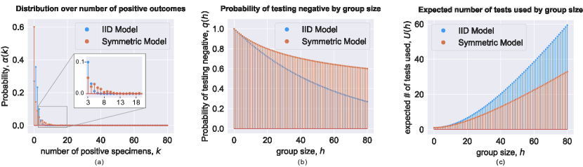
Figure 2: Comparison of an independent and identically distributed (IID) model with a symmetric model for a population of size 80. (a) The representation $\alpha$ of these distributions where $\alpha(k)$ is the probability of seeing $k$ positive specimens (see Proposition 3.2). The IID model decays more rapidly. The symmetric distribution has non-monotonic decay; e.g., it assigns more mass to five positives than four positives. (b) The representation $q$ where $q(h)$ is the probability that a group of size $h$ tests negative (see Lemma 3.4). The IID model underestimates these probabilities. (c) The function $U$ where $U(h)$ is the expected number of tests used on a group of size $h$ (see Lemma 4.6). The IID model overestimates these costs.

Pooling strategies

Strategies (1), (2) and (3) each indicate 10 pools of size 8 whereas strategy (4) indicates 8 pools of size 10. Since the strategies only indicate two distinct poolings, we refer to size-8 pools and size-10 pools in the discussion below.

Theoretical efficiencies

Both Dorfman’s infinite analysis and the finite IID model indicate an efficiency of 4.04 for size-8 pools. Under the estimated symmetric model, the efficiency of the size-8 and size-10 pools is 4.38 and 4.48, respectively.

Empirical efficiencies

The average empirical efficiencies of the size-8 and size-10 pools are 4.38 and 4.48, respectively. The standard error in both cases is 0.02. Without randomization, the empirical efficiencies for size-8 and size-10 pools are 4.71 and 4.75, respectively.

5.5 Discussion and interpretation

The estimated IID and symmetric distributions differ visibly (see Figure 2). The IID distribution underestimates the probabilities of observing $\geq 6$ positive specimens (see Figure 2, panel a). Hence, it also the underestimates probability that a group of a particular size will test negative (see Figure 2, panel b). As a result, it overestimates the number of tests used for a group of a particular size (see Figure 2, panel c).

Strategies

The first three strategies coincide whereas strategy (4) uses fewer and larger pools. In our experience, it is usual for the symmetric model to indicate larger pools. We attribute this phenomenon to the overestimation described in the previous paragraph.

We emphasize that strategies (1), (2) and (3) need not coincide. When they do differ, in our experience, it is often by indicating successively larger pools. For example, strategy (3) avoids the small remainder pool indicated by (2) when Dorfman’s pool size does not evenly divide the population size. Here the strategies agree. They also agree with the Hebrew University team’s original choice of size-8 pools.

Theoretical efficiencies

The efficiencies indicated by Dorfman and the finite IID model (a) agree, (b) exceed that reported in [21] and (c) underestimate the theoretical efficiency as predicted by the symmetric distribution. Phenomenon (a) may be interpreted to justify Dorfman’s approximation. Phenomenon (b) occurs because the prevalence is slightly lower in our processed data than the original dataset. Phenomenon (c) is a consequence of the IID model overestimating the expected number of tests used.

Under the estimated symmetric distribution, the efficiency of the size-10 pools exceeds that of the size-8 pools. We expect the size-10 pools to be at least as efficient as the size-8 pools as a consequence of the optimization carried out in strategy (4).

Empirical efficiencies

With randomization, the mean empirical efficiencies agree with their theoretical values. The standard errors are relatively small.

Without randomization, both size-8 and size-10 efficiencies increase with the size-10 efficiency remaining larger. This increase appears to be a consequence of the intentional pooling carried out by the Hebrew University Team. Since we batch and pool sequentially, the size-8 pools used here match exactly those constructed by the team. Although the size-10 efficiency is higher here, our experience indicates that this is not significant. The empirical efficiency reported in [21] is lower than these values because certain pools were retested even though each of the pool’s specimens was negative.

6 Conclusion

In this paper, we develop and apply tools for Dorfman’s two-stage adaptive group testing protocol. In particular, we study the problem under the modeling assumption that the statuses are exchangeable and so their distribution is symmetric.

This modeling assumption is both amenable to analysis and relevant for infectious disease screening. Although symmetric distributions are a simple model of reality, they nonetheless allow for correlation among specimen statuses. Such correlations appear in disease screening because specimens originating from the same family, living space, or workplace often arrive for testing, and hence for pooling, together. Since the disease is contagious, positive statuses co-occur. Accounting for this phenomenon in the probabilistic model may indicate better efficiency and larger pool sizes than proposed by the classical theory. The dataset we studied in Section 5 exhibits this feature. In summary, symmetric distributions are a prototypical class on the path to further research into and analysis of more complicated models.

6.1 Future directions

We focus on topics related to Dorfman’s procedure. It may also be of interest, however, to analyze other group testing protocols, e.g. Sterrett’s procedure [168] or Sobel and Groll’s binary splitting [162], under exchangeability.

Notable variants and generalization

We list three variants and a generalization of the symmetry considered in this paper. The three variants are (1) infinite population exchangeability, (2) test error models for exchangeable statuses, and (3) risk-adjusted objectives incorporating, e.g., the variance of the number of tests used. Even within the finite population, error-free, minimize-expected-tests setting of this paper, an interesting generalization of this paper may study distributions which are invariant under an arbitrary permutation group.

Characterizing savings and robustness

How much can we save by correctly modeling statuses as exchangeable instead of independent? Toward answering this, suppose $x$ has symmetric distribution $p$ and denote by $\bar{p}$ the IID distribution whose prevalence matches that of $p$. Suppose $G^{\star}$ and $\bar{G}^{\star}$ are the corresponding optimal partitions under $p$ and $\bar{p}$, respectively. One approach to the question of savings is to study the quantity $\Delta(p):=\mathbb{E}C(\bar{G}^{\star},x)-\mathbb{E}C(G^{\star},x)$. What is $\sup_{p}\Delta(p)$? Which symmetric distributions achieve this? There are no savings if $\bar{G}^{\star}=G^{\star}$, but Section 5 indicates that distributions with savings exist and appear empirically.

Also, how robust are these approaches to uncertainty in estimated parameters. Given an interval containing the population prevalence or a set containing the symmetric distribution, what are the optimal worst-case partitions? The linear programming approach (see Section 4.4.1) may be useful for these questions and the foregoing one.

Using features to estimate the probability a group tests negative

Lastly, we sketch a direction toward more complicated distributions. Although specimens have identical marginals under the symmetric models considered in this paper, it is natural to relax this assumption as well. Classically, Hwang [90] proposed using specimen-specific negative-status probabilities. He showed that, assuming independence, one can efficiently compute partitions to minimize the expected number of tests used. With modern tools, one might use features and logistic regression to estimate these probabilities. See [30] for an approach along these lines.

To generalize, one may drop the independence assumption and directly estimate the probability that a group tests negative by, for example, performing logistic regression on sets of individual specimen features. Regression models that do not depend on the order of an input list of feature vectors are called permutation-invariant [185, 32]. Given such a model indicating the probability that a group tests negative, one might then employ general-purpose partitioning algorithms to find partitions which minimize the expected number of tests used.

References

- [1] B. Abdalhamid, C. R. Bilder, E. L. McCutchen, S. H. Hinrichs, S. A. Koepsell, and P. C. Iwen, Assessment of specimen pooling to conserve SARS CoV-2 testing resources, American Journal of Clinical Pathology, 153 (2020), pp. 715–718, https://doi.org/10.1093/ajcp/aqaa064.
- [2] L. Abraham, G. Becigneul, B. Coleman, B. Scholkopf, A. Shrivastava, and A. Smola, Bloom origami assays: Practical group testing, 2020, https://arxiv.org/abs/2008.02641.
- [3] S. Ahn, W.-N. Chen, and A. Özgür, Adaptive group testing on networks with community structure, in 2021 IEEE International Symposium on Information Theory (ISIT), 2021, pp. 1242–1247, https://doi.org/10.1109/ISIT45174.2021.9517888.
- [4] S. Ahn, W.-N. Chen, and A. Özgür, Adaptive group testing on networks with community structure: The stochastic block model, IEEE Transactions on Information Theory, 69 (2023), pp. 4758–4776, https://doi.org/10.1109/TIT.2023.3247520.
- [5] D. J. Aldous, Exchangeability and related topics, in École d’Été de Probabilités de Saint-Flour XIII — 1983, Berlin, Heidelberg, 1985, Springer Berlin Heidelberg, pp. 1–198, https://doi.org/10.1007/BFb0099421.
- [6] M. Aldridge, Conservative two-stage group testing in the linear regime, 2022, https://doi.org/10.48550/arXiv.2005.06617, https://arxiv.org/abs/2005.06617.
- [7] M. Aldridge, O. Johnson, and J. Scarlett, Group testing: An information theory perspective, Foundations and Trends in Communications and Information Theory, 15 (2019), pp. 196–392, https://doi.org/10.1561/0100000099.
- [8] G. E. Andrews, The Theory of Partitions, Encyclopedia of Mathematics and its Applications, Cambridge University Press, 1984, https://doi.org/10.1017/CBO9780511608650.
- [9] S. Anily and A. Federgruen, Structured partitioning problems, Operations Research, 39 (1991), pp. 130–149, https://doi.org/10.1287/opre.39.1.130.
- [10] H. Aprahamian, D. R. Bish, and E. K. Bish, Optimal risk-based group testing, Management Science, 65 (2019), pp. 4365–4384, https://doi.org/10.1287/mnsc.2018.3138.
- [11] B. Arasli, Group Testing in Structured and Dynamic Networks, PhD thesis, University of Maryland, College Park, 2023.
- [12] B. Arasli and S. Ulukus, Graph and cluster formation based group testing, in 2021 IEEE International Symposium on Information Theory (ISIT), 2021, pp. 1236–1241, https://doi.org/10.1109/ISIT45174.2021.9518128.
- [13] B. Arasli and S. Ulukus, Group testing with a dynamic infection spread, in 2022 IEEE International Symposium on Information Theory (ISIT), 2022, pp. 2249–2254, https://doi.org/10.1109/ISIT50566.2022.9834486.
- [14] B. Arasli and S. Ulukus, Dynamic infection spread model based group testing, Algorithms, 16 (2023).
- [15] M. A. Attia, W.-T. Chang, and R. Tandon, Heterogeneity aware two-stage group testing, IEEE Transactions on Signal Processing, 69 (2021), pp. 3977–3990, https://doi.org/10.1109/TSP.2021.3093785.
- [16] N. Augenblick, J. T. Kolstad, Z. Obermeyer, and A. Wang, Group testing in a pandemic: The role of frequent testing, correlated risk, and machine learning, tech. report, National Bureau of Economic Research, 2020, https://doi.org/10.3386/w27457.
- [17] D. Austin, Pooling strategies for COVID-19 testing, 2020, http://www.ams.org/publicoutreach/feature-column/fc-2020-10.
- [18] M. Baccini, E. Rocco, I. Paganini, A. Mattei, C. Sani, G. Vannucci, S. Bisanzi, E. Burroni, M. Peluso, A. Munnia, F. Cellai, G. Pompeo, L. Micio, J. Viti, F. Mealli, and F. M. Carozzi, Pool testing on random and natural clusters of individuals: Optimisation of sars-cov-2 surveillance in the presence of low viral load samples, PLOS ONE, 16 (2021), pp. 1–15, https://doi.org/10.1371/journal.pone.0251589.
- [19] E. Balas and M. W. Padberg, Set partitioning: A survey, SIAM Review, 18 (1976), pp. 710–760, https://doi.org/10.1137/1018115.
- [20] D. J. Balding and D. C. Torney, Optimal pooling designs with error detection, Journal of Combinatorial Theory, Series A, 74 (1996), pp. 131–140, https://doi.org/10.1006/jcta.1996.0041.
- [21] N. Barak, R. Ben-Ami, T. Sido, A. Perri, A. Shtoyer, M. Rivkin, T. Licht, A. Peretz, J. Magenheim, I. Fogel, A. Livneh, Y. Daitch, E. Oiknine-Djian, G. Benedek, Y. Dor, D. G. G., M. Yassour, et al., Lessons from applied large-scale pooling of 133,816 SARS-CoV-2 RT-PCR tests, Science Translational Medicine, 13 (2021), https://doi.org/10.1126/scitranslmed.abf2823.
- [22] H. W. Becker and J. Riordan, The arithmetic of bell and stirling numbers, American Journal of Mathematics, 70 (1948), pp. 385–394, https://doi.org/10.2307/2372336.
- [23] R. Ben-Ami, A. Klochendler, M. Seidel, T. Sido, O. Gurel-Gurevich, M. Yassour, E. Meshorer, G. Benedek, I. Fogel, E. Oiknine-Djian, A. Gertler, Z. Rotstein, B. Lavi, Y. Dor, D. Wolf, M. Salton, Y. Drier, A. Klochendler, A. Eden, A. Klar, A. Geldman, A. Arbel, A. Peretz, B. Shalom, B. Ochana, D. Avrahami-Tzfati, D. Neiman, D. Steinberg, D. B. , E. Shpigel, G. Atlan, H. Klein, H. Chekroun, H. Shani, I. Hazan, I. Ansari, I. Magenheim, J. Moss, J. Magenheim, L. Peretz, L. Feigin, M. Saraby, M. Sherman, M. Bentata, M. Avital, M. Kott, M. Peyser, M. Weitz, M. Shacham, M. Grunewald, N. Sasson, N. Wallis, N. Azazmeh, N. Tzarum, O. Fridlich, R. Sher, R. Condiotti, R. Refaeli, R. Ben Ami, R. Zaken-Gallili, R. Helman, S. Ofek, S. Tzaban, S. Piyanzin, S. Anzi, S. Dagan, S. Lilenthal, T. Sido, T. Licht, T. Friehmann, Y. Kaufman, A. Pery, A. Saada, A. Dekel, A. Yeffet, A. Shaag, A. Michael-Gayego, E. Shay, E. Arbib, H. Onallah, K. Ben-Meir, L. Levinzon, L. Cohen-Daniel, L. Natan, M. Hamdan, M. Rivkin, M. Shwieki, O. Vorontsov, R. Barsuk, R. Abramovitch, R. Gutorov, S. Sirhan, S. Abdeen, Y. Yachnin, and Y. Daitch, Large-scale implementation of pooled RNA extraction and RT-PCR for SARS-CoV-2 detection, Clinical Microbiology and Infection, 26 (2020), pp. 1248–1253, https://doi.org/10.1016/j.cmi.2020.06.009.
- [24] T. Berger and V. I. Levenshtein, Asymptotic efficiency of two-stage disjunctive testing, IEEE Transactions on Information Theory, 48 (2002), pp. 1741–1749, https://doi.org/10.1109/TIT.2002.1013122.
- [25] T. Berger, N. Mehravari, D. Towsley, and J. Wolf, Random multiple-access communication and group testing, IEEE Transactions on Communications, 32 (1984), pp. 769–779, https://doi.org/10.1109/TCOM.1984.1096146.
- [26] P. Bertolotti, Inference and Diffusion in Networks, PhD thesis, Massachusetts Institute of Technology, February 2022.
- [27] P. Bertolotti and A. Jadbabaie, Network group testing, 2021, https://arxiv.org/abs/2012.02847.
- [28] A. F. Best, Y. Malinovsky, and P. S. Albert, The efficient design of nested group testing algorithms for disease identification in clustered data, Journal of Applied Statistics, 50 (2023), pp. 2228–2245, https://doi.org/10.1080/02664763.2022.2071419.
- [29] X. Bi, E. Miehling, C. Beck, and T. Başar, Approximate testing in uncertain epidemic processes, in 2022 IEEE 61st Conference on Decision and Control (CDC), 2022, pp. 4339–4344, https://doi.org/10.1109/CDC51059.2022.9992464.
- [30] C. R. Bilder, J. T. M., and P. Chen, Informative retesting, Journal of the American Statistical Association, 105 (2010), pp. 942–955, https://doi.org/10.1198/jasa.2010.ap09231.
- [31] M. S. Black, C. R. Bilder, and J. M. Tebbs, Group testing in heterogeneous populations by using halving algorithms, Journal of the Royal Statistical Society. Series C (Applied Statistics), 61 (2012), pp. 277–290, http://www.jstor.org/stable/41430963.
- [32] B. Bloem-Reddy and Y. W. Teh, Probabilistic symmetries and invariant neural networks, J. Mach. Learn. Res., 21 (2020).
- [33] A. Z. Broder and R. Kumar, A note on double pooling tests, 2020.
- [34] W. Bruno, E. Knill, D. Balding, D. Bruce, N. Doggett, W. Sawhill, R. Stallings, C. Whittaker, and D. Torney, Efficient pooling designs for library screening, Genomics, 26 (1995), pp. 21–30, https://doi.org/10.1016/0888-7543(95)80078-Z.
- [35] S.-J. Cao, R. Goenka, C.-W. Wong, A. Rajwade, and D. Baron, Group testing with side information via generalized approximate message passing, IEEE Transactions on Signal Processing, 71 (2023), pp. 2366–2375, https://doi.org/10.1109/TSP.2023.3287671.
- [36] C. L. Chan, P. H. Che, S. Jaggi, and V. Saligrama, Non-adaptive probabilistic group testing with noisy measurements: Near-optimal bounds with efficient algorithms, in 2011 49th Annual Allerton Conference on Communication, Control, and Computing (Allerton), 2011, pp. 1832–1839, https://doi.org/10.1109/Allerton.2011.6120391.
- [37] G. J. Chang and F. K. Hwang, A group testing problem, SIAM Journal on Algebraic Discrete Methods, 1 (1980), pp. 21–24, https://doi.org/10.1137/0601004.
- [38] G. J. Chang and F. K. Hwang, A group testing problem on two disjoint sets, SIAM Journal on Algebraic Discrete Methods, 2 (1981), pp. 35–38, https://doi.org/10.1137/0602005.
- [39] C. L. Chen and W. H. Swallow, Using group testing to estimate a proportion, and to test the binomial model, Biometrics, 46 (1990), pp. 1035–1046, https://doi.org/10.2307/2532446.
- [40] M. Cheraghchi, A. Hormati, A. Karbasi, and M. Vetterli, Group testing with probabilistic tests: Theory, design and application, IEEE Transactions on Information Theory, 57 (2011), pp. 7057–7067, https://doi.org/10.1109/TIT.2011.2148691.
- [41] M. Cheraghchi, A. Karbasi, S. Mohajer, and V. Saligrama, Graph-constrained group testing, IEEE Transactions on Information Theory, 58 (2012), pp. 248–262, https://doi.org/10.1109/TIT.2011.2169535.
- [42] A. Cohen, A. Cohen, and O. Gurewitz, Efficient data collection over multiple access wireless sensors network, IEEE/ACM Transactions on Networking, 28 (2020), pp. 491–504, https://doi.org/10.1109/TNET.2020.2964764.
- [43] A. Cohen, N. Shlezinger, S. Salamatian, Y. C. Eldar, and M. Médard, Serial quantization for sparse time sequences, IEEE Transactions on Signal Processing, 69 (2021), pp. 3299–3314, https://doi.org/10.1109/TSP.2021.3083985.
- [44] S. Comess, H. Wang, S. Holmes, and C. Donnat, Statistical modeling for practical pooled testing during the COVID-19 pandemic, Statistical Science, 37 (2022), pp. 229–250, https://doi.org/10.1214/22-STS857.
- [45] G. Cormode and S. Muthukrishnan, What’s hot and what’s not: Tracking most frequent items dynamically, ACM Trans. Database Syst., 30 (2005), pp. 249–278, https://doi.org/10.1145/1061318.1061325.
- [46] E. A. Daniel, B. H. Esakialraj L, A. S, K. Muthuramalingam, R. Karunaianantham, L. P. Karunakaran, M. Nesakumar, M. Selvachithiram, S. Pattabiraman, S. Natarajan, S. P. Tripathy, and L. E. Hanna, Pooled testing strategies for sars-cov-2 diagnosis: A comprehensive review, Diagnostic Microbiology and Infectious Disease, 101 (2021), https://doi.org/10.1016/j.diagmicrobio.2021.115432.
- [47] A. De Bonis, L. Gasieniec, and U. Vaccaro, Optimal two-stage algorithms for group testing problems, SIAM Journal on Computing, 34 (2005), pp. 1253–1270, https://doi.org/10.1137/S0097539703428002.
- [48] B. de Finetti, Funzione caratteristica di un fenomeno aleatorio, Memorie. Academia Nazionale del Linceo, 6 (1931), pp. 251–299.
- [49] B. De Finetti, Probability, Induction and Statistics: The Art of Guessing, Wiley, 1972.
- [50] A. Deckert, T. Bärnighausen, and N. Kyei, Simulation of pooled-sample analysis strategies for covid-19 mass testing, Bulletin of the World Health Organization, 98 (2020), pp. 590–598, https://doi.org/10.2471/BLT.20.257188.
- [51] P. Diaconis, Finite forms of de finetti’s theorem on exchangeability, Synthese, 36 (1977), pp. 271–281, https://doi.org/10.1007/BF00486116.
- [52] P. Diaconis and D. Freedman, Finite exchangeable sequences, The Annals of Probability, 8 (1980), pp. 745–764.
- [53] M. Doger and S. Ulukus, Group testing with non-identical infection probabilities, in 2021 XVII International Symposium “Problems of Redundancy in Information and Control Systems” (REDUNDANCY), 2021, pp. 110–115, https://doi.org/10.1109/REDUNDANCY52534.2021.9606443.
- [54] M. Doger and S. Ulukus, Dynamical dorfman testing with quarantine, in 2022 56th Annual Conference on Information Sciences and Systems (CISS), 2022, pp. 31–36, https://doi.org/10.1109/CISS53076.2022.9751175.
- [55] R. Dorfman, The detection of defective members of large populations, The Annals of Mathematical Statistics, 14 (1943), pp. 436–440, https://doi.org/10.1214/aoms/1177731363.
- [56] D. Du and F. K. Hwang, Combinatorial group testing and its applications, vol. 12 of Applied Mathematics, World Scientific, 2nd ed., 2000, https://doi.org/10.1142/4252.
- [57] A. G. D’yachkov, Lectures on designing screening experiments, 2014, https://arxiv.org/abs/1401.7505.
- [58] H. El Hajj, D. R. Bish, E. K. Bish, and H. Aprahamian, Screening multi-dimensional heterogeneous populations for infectious diseases under scarce testing resources, with application to COVID-19, Naval Research Logistics (NRL), 69 (2022), pp. 3–20, https://doi.org/10.1002/nav.21985.
- [59] J. Ellenberg, Five people. one test. this is how you get there., 2020, https://www.nytimes.com/2020/05/07/opinion/coronavirus-group-testing.html.
- [60] A. Emad and O. Milenkovic, Poisson group testing: A probabilistic model for nonadaptive streaming boolean compressed sensing, in 2014 IEEE International Conference on Acoustics, Speech and Signal Processing (ICASSP), 2014, pp. 3335–3339, https://doi.org/10.1109/ICASSP.2014.6854218.
- [61] A. Emad and O. Milenkovic, Semiquantitative group testing, IEEE Transactions on Information Theory, 60 (2014), pp. 4614–4636, https://doi.org/10.1109/TIT.2014.2327630.
- [62] K. Engel, T. Radzik, and J.-C. Schlage-Puchta, Optimal integer partitions, European Journal of Combinatorics, 36 (2014), pp. 425–436, https://doi.org/10.1016/j.ejc.2013.09.004.
- [63] D. Eppstein, M. T. Goodrich, and D. S. Hirschberg, Improved combinatorial group testing algorithms for real‐world problem sizes, SIAM Journal on Computing, 36 (2007), pp. 1360–1375, https://doi.org/10.1137/050631847.
- [64] W. A. Ericson, A bayesian approach to two-stage sampling, tech. report, University of Michigan, Ann Arbor, Department of Statistics, 1976.
- [65] M. Farach, S. Kannan, E. Knill, and S. Muthukrishnan, Group testing problems with sequences in experimental molecular biology, in Proceedings. Compression and Complexity of SEQUENCES 1997 (Cat. No.97TB100171), 1997, pp. 357–367, https://doi.org/10.1109/SEQUEN.1997.666930.
- [66] W. Feller, An Introduction to Probability Theory and Its Applications, vol. 1, John Wiley, New York, 3rd ed., 1968.
- [67] H. M. Finucan, The blood testing problem, Journal of the Royal Statistical Society. Series C (Applied Statistics), 13 (1964), pp. 43–50, https://doi.org/10.2307/2985222.
- [68] D. Freedman, Some Issues in the Foundation of Statistics, Springer Netherlands, Dordrecht, 1997, pp. 19–39, https://doi.org/10.1007/978-94-015-8816-4_4.
- [69] V. Gandikota, E. Grigorescu, S. Jaggi, and S. Zhou, Nearly optimal sparse group testing, in 2016 54th Annual Allerton Conference on Communication, Control, and Computing (Allerton), 2016, pp. 401–408, https://doi.org/10.1109/ALLERTON.2016.7852259.
- [70] V. Gandikota, E. Grigorescu, S. Jaggi, and S. Zhou, Nearly optimal sparse group testing, IEEE Transactions on Information Theory, 65 (2019), pp. 2760–2773, https://doi.org/10.1109/TIT.2019.2891651.
- [71] M. R. Garey and D. S. Johnson, Computers and Intractability: A Guide to the Theory of NP-Completeness, Books in the Mathematical Sciences, W. H. Freeman, 1979.
- [72] S. Ghosh, R. Agarwal, M. A. Rehan, S. Pathak, P. Agarwal, Y. Gupta, S. Consul, N. Gupta, Ritika, R. Goenka, A. Rajwade, and M. Gopalkrishnan, A compressed sensing approach to pooled RT-PCR testing for COVID-19 detection, IEEE Open Journal of Signal Processing, 2 (2021), pp. 248–264, https://doi.org/10.1109/OJSP.2021.3075913.
- [73] A. C. Gilbert, M. A. Iwen, and M. J. Strauss, Group testing and sparse signal recovery, in 2008 42nd Asilomar Conference on Signals, Systems and Computers, 2008, pp. 1059–1063, https://doi.org/10.1109/ACSSC.2008.5074574.
- [74] A. Gill and D. Gottlieb, The identification of a set by successive intersections, Information and Control, 24 (1974), pp. 20–35, https://doi.org/10.1016/S0019-9958(74)80020-3.
- [75] C. Z. Gilstein, Optimal partitions of finite populations for dorfman-type group testing, Journal of Statistical Planning and Inference, 12 (1985), pp. 385–394, https://doi.org/10.1016/0378-3758(85)90087-4.
- [76] R. Goenka, S.-J. Cao, C.-W. Wong, A. Rajwade, and D. Baron, Contact tracing enhances the efficiency of COVID-19 group testing, in ICASSP 2021 - 2021 IEEE International Conference on Acoustics, Speech and Signal Processing (ICASSP), 2021, pp. 8168–8172, https://doi.org/10.1109/ICASSP39728.2021.9414034.
- [77] M. Gonen, M. Langberg, and A. Sprintson, Group testing on general set-systems, in 2022 IEEE International Symposium on Information Theory (ISIT), 2022, https://doi.org/10.1109/ISIT50566.2022.9834789.
- [78] L. E. Graff and R. Roeloffs, Group testing in the presence of test error; an extension of the Dorfman procedure, Technometrics, 14 (1972), pp. 113–122, https://doi.org/10.1080/00401706.1972.10488888.
- [79] E. D. Green and M. V. Olson, Systematic screening of yeast artificial-chromosome libraries by use of the polymerase chain reaction., Proceedings of the National Academy of Sciences, 87 (1990), pp. 1213–1217, https://doi.org/10.1073/pnas.87.3.1213.
- [80] R. N. Gurnow, A note on G. S. Watson’s paper ‘A Study of the Group Screening Method”, Technometrics, 7 (1965), pp. 444–446, https://doi.org/10.1080/00401706.1965.10490276.
- [81] G. H. Hardy and E. M. Wright, An introduction to the theory of numbers, Oxford University Press, 5th ed., 1979.
- [82] N. J. Harvey, M. Patrascu, Y. Wen, S. Yekhanin, and V. W. Chan, Non-adaptive fault diagnosis for all-optical networks via combinatorial group testing on graphs, in IEEE INFOCOM 2007 - 26th IEEE International Conference on Computer Communications, 2007, pp. 697–705, https://doi.org/10.1109/INFCOM.2007.87.
- [83] J. Hayes, An adaptive technique for local distribution, IEEE Transactions on Communications, 26 (1978), pp. 1178–1186, https://doi.org/10.1109/TCOM.1978.1094204.
- [84] E. Hewitt and L. J. Savage, Symmetric measures on cartesian products, Transactions of the American Mathematical Society, 80 (1955), pp. 470–501, https://doi.org/10.2307/1992999.
- [85] B. D. Hitt, C. R. Bilder, J. M. Tebbs, and C. S. McMahan, The objective function controversy for group testing: Much ado about nothing?, Statistics in medicine, 38 (2019), pp. 4912–4923, https://doi.org/10.1002/sim.8341.
- [86] C. A. Hogan, M. K. Sahoo, and B. A. Pinsky, Sample pooling as a strategy to detect community transmission of SARS-CoV-2, Journal of the American Medical Association (JAMA), 323 (2020), pp. 1967–1969, https://doi.org/10.1001/jama.2020.5445.
- [87] D. Hong, R. Dey, X. Lin, B. Cleary, and E. Dobriban, Group testing via hypergraph factorization applied to COVID-19, Nature Communications, 13 (2022).
- [88] F. K. Hwang, A method for detecting all defective members in a population by group testing, Journal of the American Statistical Association, 67 (1972), pp. 605–608, https://doi.org/10.1080/01621459.1972.10481257.
- [89] F. K. Hwang, On finding a single defective in binomial group testing, Journal of the American Statistical Association, 69 (1974), pp. 146–150, https://doi.org/10.1080/01621459.1974.10480141.
- [90] F. K. Hwang, A generalized binomial group testing problem, Journal of the American Statistical Association, 70 (1975), pp. 923–926, https://doi.org/10.1080/01621459.1975.10480324.
- [91] F. K. Hwang, Group testing with a dilution effect, Biometrika, 63 (1976), pp. 671–680, https://doi.org/10.1093/biomet/63.3.671.
- [92] F. K. Hwang, An optimum nested procedure in binomial group testing, Biometrics, 32 (1976), pp. 939–943, https://doi.org/10.2307/2529277.
- [93] F. K. Hwang, A note on hypergeometric group testing procedures, SIAM Journal on Applied Mathematics, 34 (1978), pp. 371–375, https://doi.org/10.1137/0134030.
- [94] F. K. Hwang, Optimal group testing procedures for identifying a single defective from a finite population, Bulletin of the Institute of Mathematics Academia Sinica, 8 (1980), pp. 129–140.
- [95] F. K. Hwang, Optimal partitions, Journal of Optimization Theory and Applications, 34 (1981), https://doi.org/10.1007/BF00933355.
- [96] F. K. Hwang, Robust group testing, Journal of Quality Technology, 16 (1984), pp. 189–195, https://doi.org/10.1080/00224065.1984.11978917.
- [97] F. K. Hwang and U. G. Rothblum, Partitions: optimality and clustering (v. 1 Single-parameter), vol. 19 of Applied Mathematics, World Scientific, 2011, https://doi.org/10.1142/6518.
- [98] F. K. Hwang, T. T. Song, and D. Z. Du, Hypergeometric and generalized hypergeometric group testing, SIAM Journal on Algebraic Discrete Methods, 2 (1981), pp. 426–428, https://doi.org/10.1137/0602045.
- [99] F. K. Hwang, J. Sun, and E. Y. Yao, Optimal set partitioning, SIAM Journal on Algebraic Discrete Methods, 6 (1985), pp. 163–170, https://doi.org/10.1137/0606015.
- [100] F. K. Hwang and V. T Sós, Non-adaptive hypergeometric group testing, Studia Scientiarum Mathematicarum Hungarica, 22 (1987), pp. 257–263.
- [101] F. K.-m. Hwang and D.-Z. Du, Pooling designs and nonadaptive group testing: important tools for DNA sequencing, vol. 18 of Applied Mathematics, World Scientific, 2006.
- [102] H. A. Inan, S. Ahn, P. Kairouz, and A. Ozgur, A group testing approach to random access for short-packet communication, in 2019 IEEE International Symposium on Information Theory (ISIT), 2019, pp. 96–100, https://doi.org/10.1109/ISIT.2019.8849823.
- [103] H. A. Inan, P. Kairouz, and A. Ozgur, Sparse group testing codes for low-energy massive random access, in 2017 55th Annual Allerton Conference on Communication, Control, and Computing (Allerton), 2017, pp. 658–665, https://doi.org/10.1109/ALLERTON.2017.8262800.
- [104] H. A. Inan, P. Kairouz, and A. Ozgur, Energy-limited massive random access via noisy group testing, in 2018 IEEE International Symposium on Information Theory (ISIT), 2018, pp. 1101–1105, https://doi.org/10.1109/ISIT.2018.8437557.
- [105] H. A. Inan, P. Kairouz, and A. Özgür, Sparse combinatorial group testing, IEEE Transactions on Information Theory, 66 (2020), pp. 2729–2742, https://doi.org/10.1109/TIT.2019.2951703.
- [106] N. L. Johnson, S. Kotz, and X. Wu, Inspection Errors for Attributes in Quality Control, no. 44 in Monographs on Statistics and Applied Probability, Chapman & Hall, 1991.
- [107] W. O. Johnson and L. M. Pearson, Dual screening, Biometrics, 55 (1999), pp. 867–873, https://doi.org/10.1111/j.0006-341X.1999.00867.x.
- [108] O. Kallenberg, Probabilistic Symmetries and Invariance Principles, Probability and Its Applications, Springer, 1 ed., 2005, https://doi.org/10.1007/0-387-28861-9.
- [109] A. Karbasi and M. Zadimoghaddam, Sequential group testing with graph constraints, in 2012 IEEE Information Theory Workshop, 2012, pp. 292–296, https://doi.org/10.1109/ITW.2012.6404678.
- [110] R. M. Karp, Reducibility among Combinatorial Problems, The IBM Research Symposia Series, Springer, Boston, MA, 1972, pp. 85–103, https://doi.org/10.1007/978-1-4684-2001-2_9.
- [111] G. O. H. Katona, Combinatorial search problems, in A survey of combinatorial theory, North-Holland Publishing Company, 1973, pp. 285–308, https://doi.org/10.1016/B978-0-7204-2262-7.50028-4.
- [112] T. Kealy, O. Johnson, and R. Piechocki, The capacity of non-identical adaptive group testing, in 2014 52nd Annual Allerton Conference on Communication, Control, and Computing (Allerton), 2014, pp. 101–108, https://doi.org/10.1109/ALLERTON.2014.7028442.
- [113] D. G. Kendall, On finite and infinite sequences of exchangeable events, Studia Sci. Math. Hung, 2 (1967), pp. 319–327.
- [114] H.-Y. Kim, M. G. Hudgens, J. M. Dreyfuss, D. J. Westreich, and C. D. Pilcher, Comparison of group testing algorithms for case identification in the presence of test error, Biometrics, 63 (2007), pp. 1152–1163, https://doi.org/10.1111/j.1541-0420.2007.00817.x.
- [115] J. F. C. Kingman, Uses of exchangeability, The Annals of Probability, 6 (1978), pp. 183–197, https://doi.org/10.1214/aop/1176995566.
- [116] B. Korte and J. Vygen, Combinatorial Optimization, vol. 21 of Algorithms and Combinatorics, Springer, sixth ed., 2018, https://doi.org/10.1007/978-3-662-56039-6.
- [117] S. Kumar, Group-testing to classify all units in a trinomial sample, Studia Scientiarum Mathematicarum Hungarica, 5 (1970), pp. 247–229.
- [118] S. Kumar, Multinomial group-testing, SIAM Journal on Applied Mathematics, 19 (1970), pp. 340–350.
- [119] S. Kumar and M. Sobel, Finding a single defective in binomial group-testing, Journal of the American Statistical Association, 66 (1971), pp. 824–828, https://doi.org/10.1080/01621459.1971.10482351.
- [120] S. Kumar and M. Sobel, An asymptotically optimal bayes solution for group-testing, Tech. Report 200, University of Minnesota, 1973.
- [121] R. Lamarche-Perrin, Y. Demazeau, and J.-M. Vincent, A generic algorithmic framework to solve special versions of the set partitioning problem, in 2014 IEEE 26th International Conference on Tools with Artificial Intelligence, 2014, pp. 891–897, https://doi.org/10.1109/ICTAI.2014.136.
- [122] N. C. Landolfi, Symgt: A package for group testing against symmetric distributions, 2023, https://pypi.org/project/symgt/.
- [123] I. Lau, J. Scarlett, and Y. Sun, Model-based and graph-based priors for group testing, IEEE Transactions on Signal Processing, 70 (2022), pp. 6035–6050, https://doi.org/10.1109/TSP.2022.3229942.
- [124] E. L. Lawler, Combinatorial Optimization: Networks and Matroids, Holt, Rinehart and Winston, 1976.
- [125] J.-K. Lee and M. Sobel, Dorfman and R1-type procedures for a generalized group-testing problem, Mathematical Biosciences, 15 (1972), pp. 317–340, https://doi.org/10.1016/0025-5564(72)90040-5.
- [126] S. D. Lendle, M. G. Hudgens, and B. F. Qaqish, Group testing for case identification with correlated responses, Biometrics, 68 (2012), pp. 532–540.
- [127] C. H. Li, A sequential method for screening experimental variables, Journal of the American Statistical Association, 57 (1962), pp. 455–477, https://doi.org/10.1080/01621459.1962.10480672.
- [128] T. Li, C. L. Chan, W. Huang, T. Kaced, and S. Jaggi, Group testing with prior statistics, in 2014 IEEE International Symposium on Information Theory, 2014, pp. 2346–2350, https://doi.org/10.1109/ISIT.2014.6875253.
- [129] Y.-J. Lin, C.-H. Yu, T.-H. Liu, C.-S. Chang, and W.-T. Chen, Positively correlated samples save pooled testing costs, IEEE Transactions on Network Science and Engineering, 8 (2021), pp. 2170–2182, https://doi.org/10.1109/TNSE.2021.3081759.
- [130] S. Lohse, T. Pfuhl, B. Berkó-Göttel, J. Rissland, T. Geißler, B. Gärtner, S. L. Becker, S. Schneitler, and S. Smola, Pooling of samples for testing for SARS-CoV-2 in asymptomatic people, The Lancet Infectious Diseases, 20 (2020), pp. 1231–1232, https://doi.org/10.1016/S1473-3099(20)30362-5.
- [131] J. Luo and D. Guo, Neighbor discovery in wireless ad hoc networks based on group testing, in 2008 46th Annual Allerton Conference on Communication, Control, and Computing, 2008, pp. 791–797, https://doi.org/10.1109/ALLERTON.2008.4797638.
- [132] I. G. Macdonald, Symmetric functions and Hall polynomials, Clarendon Press, second ed., 1998.
- [133] A. J. Macula, Probabilistic nonadaptive and two-stage group testing with relatively small pools and DNA library screening, Journal of Combinatorial Optimization, 2 (1998), pp. 385–397, https://doi.org/10.1023/A:1009732820981.
- [134] Y. Malinovsky and P. S. Albert, Revisiting nested group testing procedures: New results, comparisons, and robustness, The American Statistician, 73 (2019), pp. 117–125, https://doi.org/10.1080/00031305.2017.1366367.
- [135] D. Malioutov and K. Varshney, Exact rule learning via boolean compressed sensing, in Proceedings of the 30th International Conference on Machine Learning, S. Dasgupta and D. McAllester, eds., vol. 28 of Proceedings of Machine Learning Research, Atlanta, Georgia, USA, 17–19 Jun 2013, PMLR, pp. 765–773.
- [136] S. Mallapaty, The mathematical strategy that could transform coronavirus testing, Nature, 583 (2020), pp. 504–505.
- [137] C. S. McMahan, J. M. Tebbs, and C. R. Bilder, Informative dorfman screening, Biometrics, 68 (2012), pp. 287–296, https://doi.org/10.1111/j.1541-0420.2011.01644.x.
- [138] C. S. McMahan, J. M. Tebbs, and C. R. Bilder, Two-dimensional informative array testing, Biometrics, 68 (2012), pp. 793–804, https://doi.org/10.1111/j.1541-0420.2011.01726.x.
- [139] N. Mehravari, Generalized binary binomial group testing, SIAM Journal on Algebraic Discrete Methods, 7 (1986), pp. 159–166, https://doi.org/10.1137/0607019.
- [140] L. Mutesa, P. Ndishimye, Y. Butera, J. Souopgui, A. Uwineza, R. Rutayisire, E. L. Ndoricimpaye, E. Musoni, N. Rujeni, T. Nyatanyi, et al., A pooled testing strategy for identifying SARS-CoV-2 at low prevalence, Nature, 589 (2021), pp. 276–280, https://doi.org/10.1038/s41586-020-2885-5.
- [141] M. Mézard and C. Toninelli, Group testing with random pools: Optimal two-stage algorithms, IEEE Transactions on Information Theory, 57 (2011), pp. 1736–1745, https://doi.org/10.1109/TIT.2010.2103752.
- [142] National Center for Immunization and Respiratory Diseases (U.S.). Division of Viral Diseases, Interim guidance for use of pooling procedures in sars-cov-2 diagnostic, screening, and surveillance testing, July 2020, https://stacks.cdc.gov/view/cdc/90937.
- [143] E. Nebenzahl and M. Sobel, Finite and infinite models for generalized group testing with unequal probability of success for each item, in Discriminant Analysis and Applications, Academic Press, 1973, pp. 239–278.
- [144] P. Nikolopoulos, S. R. Srinivasavaradhan, T. Guo, C. Fragouli, and S. Diggavi, Group testing for overlapping communities, in ICC 2021 - IEEE International Conference on Communications, 2021, pp. 1–7, https://doi.org/10.1109/ICC42927.2021.9500791.
- [145] P. Nikolopoulos, S. R. Srinivasavaradhan, T. Guo, C. Fragouli, and S. N. Diggavi, Community-aware group testing, IEEE Transactions on Information Theory, 69 (2023), pp. 4361–4383, https://doi.org/10.1109/TIT.2023.3250119.
- [146] H. Nikpey, J. Kim, X. Chen, S. Sarkar, and S. S. Bidokhti, Group testing with correlation under edge-faulty graphs, 2023, https://arxiv.org/abs/2202.02467.
- [147] Office of the Commissioner, Coronavirus (COVID-19) update: FDA issues first emergency authorization for sample pooling in diagnostic testing, 2020, https://www.fda.gov/news-events/press-announcements/coronavirus-covid-19-update-fda-issues-first-emergency-authorization-sample-pooling-diagnostic.
- [148] S. Onn and V. S. A., Some efficiently solvable problems over integer partition polytopes, Discrete Applied Mathematics, 180 (2015), pp. 135–140, https://doi.org/10.1016/j.dam.2014.08.015.
- [149] D. S. Pavlichin, Nearest symmetric distributions, in 2015 IEEE International Symposium on Information Theory (ISIT), IEEE, 2015, pp. 1630–1634, https://doi.org/10.1109/ISIT.2015.7282732.
- [150] C. G. Pfeifer and P. Enis, Dorfman-type group testing for a modified binomial model, Journal of the American Statistical Association, 73 (1978), pp. 588–592, https://doi.org/10.1080/01621459.1978.10480059.
- [151] R. M. Phatarfod and A. Sudbury, The use of a square array scheme in blood testing, Statistics in Medicine, 13 (1994), pp. 2337–2343, https://doi.org/10.1002/sim.4780132205.
- [152] J. Rewley, Specimen pooling to conserve additional testing resources when persons’ infection status is correlated: A simulation study, Epidemiology, 31 (2020), pp. 832–835, https://doi.org/10.1097/EDE.0000000000001244.
- [153] G.-C. Rota, The number of partitions of a set, The American Mathematical Monthly, 71 (1964), pp. 498–504, https://doi.org/10.1080/00029890.1964.11992270.
- [154] S. M. Samuels, The exact solution to the two-stage group-testing problem, Technometrics, 20 (1978), pp. 497–500, https://doi.org/10.1080/00401706.1978.10489706.
- [155] A. Schrijver, Theory of Linear and Integer Programming, John Wiley & Sons, 1998.
- [156] A. Schrijver, Combinatorial Optimization: Polyhedra and Efficiency, vol. 24 of Algorithms and Combinatorics, Springer, 2004.
- [157] D. K. Sewell, Leveraging network structure to improve pooled testing efficiency, Journal of the Royal Statistical Society Series C: Applied Statistics, 71 (2022), pp. 1648–1662, https://doi.org/10.1111/rssc.12594.
- [158] S. Sihag, A. Tajer, and U. Mitra, Adaptive graph-constrained group testing, IEEE Transactions on Signal Processing, 70 (2022), pp. 381–396, https://doi.org/10.1109/TSP.2021.3137026.
- [159] M. Sobel, Binomial and hypergeometric group-testing, Tech. Report 76, University of Minnesota, Department of Statistics, July 1966.
- [160] M. Sobel, Binomial and hypergeometric group-testing, Studia Scientiarum Mathematicarum Hungarica, 3 (1968), pp. 19–42.
- [161] M. Sobel and R. M. Elashoff, Group testing with a new goal, estimation, Biometrika, 62 (1975), pp. 181–193, https://doi.org/10.1093/biomet/62.1.181.
- [162] M. Sobel and P. A. Groll, Group testing to eliminate efficiently all defectives in a binomial sample, Bell System Technical Journal, 38 (1959), pp. 1179–1252.
- [163] M. Sobel and P. A. Groll, Binomial group-testing with an unknown proportion of defectives, Technometrics, 8 (1966), pp. 631–656, https://doi.org/10.1080/00401706.1966.10490408.
- [164] M. Sobel, S. Kumar, and S. Blumenthal, Symmetric binomial group-testing with three outcomes, in Statistical Decision Theory and Related Topics, S. S. Gupta and J. Yackel, eds., Academic Press, 1971, pp. 119–160, https://doi.org/10.1016/B978-0-12-307550-5.50011-3.
- [165] B. Spang and M. Wootters, Unconstraining Graph-Constrained Group Testing, in Approximation, Randomization, and Combinatorial Optimization. Algorithms and Techniques (APPROX/RANDOM 2019), D. Achlioptas and L. A. Végh, eds., vol. 145 of Leibniz International Proceedings in Informatics (LIPIcs), Dagstuhl, Germany, 2019, Schloss Dagstuhl–Leibniz-Zentrum fuer Informatik, pp. 46:1–46:20, https://doi.org/10.4230/LIPIcs.APPROX-RANDOM.2019.46.
- [166] S. R. Srinivasavaradhan, P. Nikolopoulos, C. Fragouli, and S. Diggavi, An entropy reduction approach to continual testing, in 2021 IEEE International Symposium on Information Theory (ISIT), 2021, pp. 611–616, https://doi.org/10.1109/ISIT45174.2021.9518188.
- [167] S. R. Srinivasavaradhan, P. Nikolopoulos, C. Fragouli, and S. Diggavi, Dynamic group testing to control and monitor disease progression in a population, in 2022 IEEE International Symposium on Information Theory (ISIT), 2022, pp. 2255–2260, https://doi.org/10.1109/ISIT50566.2022.9834823.
- [168] A. Sterrett, On the detection of defective members of large populations, The Annals of Mathematical Statistics, 28 (1957), pp. 1033–1036, https://www.jstor.org/stable/2237067.
- [169] A. F. Sunjaya and A. P. Sunjaya, Pooled testing for expanding COVID-19 mass surveillance, Disaster Medicine and Public Health Preparedness, 14 (2020), pp. e42–e43, https://doi.org/10.1017/dmp.2020.246.
- [170] J. M. Tebbs, C. S. McMahan, and C. R. Bilder, Two-stage hierarchical group testing for multiple infections with application to the infertility prevention project, Biometrics, 69 (2013), pp. 1064–1073, https://doi.org/10.1111/biom.12080.
- [171] S. Tsirtsis, A. De, L. Lorch, and M. Gomez-Rodriguez, Pooled testing of traced contacts under superspreading dynamics, PLOS Computational Biology, 18 (2022), pp. 1–17, https://doi.org/10.1371/journal.pcbi.1010008.
- [172] D. W. Turner, F. E. Tidmore, and D. M. Young, A calculus based approach to the blood testing problem, SIAM Review, 30 (1988), pp. 119–122, https://doi.org/10.1137/1030005.
- [173] S. Ubaru and A. Mazumdar, Multilabel classification with group testing and codes, in Proceedings of the 34th International Conference on Machine Learning, D. Precup and Y. W. Teh, eds., vol. 70 of Proceedings of Machine Learning Research, PMLR, 06–11 Aug 2017, pp. 3492–3501, https://proceedings.mlr.press/v70/ubaru17a.html.
- [174] P. Ungar, The cutoff point for group testing, Communications on Pure and Applied Mathematics, 13 (1960), pp. 49–54.
- [175] C. M. Verdun, T. Fuchs, P. Harar, D. Elbrächter, D. S. Fischer, J. Berner, P. Grohs, F. J. Theis, and F. Krahmer, Group testing for sars-cov-2 allows for up to 10-fold efficiency increase across realistic scenarios and testing strategies, Frontiers in Public Health, 9 (2021), https://doi.org/10.3389/fpubh.2021.583377.
- [176] J. Wan, Y. Zhang, and P. I. Frazier, Correlation improves group testing, 2022, https://doi.org/10.48550/arXiv.2111.07517, https://arxiv.org/abs/2111.07517.
- [177] D. Wang, C. S. McMahan, J. M. Tebbs, and C. R. Bilder, Group testing case identification with biomarker information, Computational Statistics & Data Analysis, 122 (2018), pp. 156–166, https://doi.org/10.1016/j.csda.2018.01.005.
- [178] H. Wang, C. A. Hogan, J. A. Miller, M. K. Sahoo, C. Huang, K. O. Mfuh, M. Sibai, J. Zehnder, B. Hickey, N. Sinnott-Armstrong, et al., Performance of nucleic acid amplification tests for detection of severe acute respiratory syndrome coronavirus 2 in prospectively pooled specimens, Emerging Infectious Diseases, 27 (2021), https://doi.org/10.3201/eid2701.203379.
- [179] H.-P. Wang, R. Gabrys, and A. Vardy, Tropical group testing, IEEE Transactions on Information Theory, (2023), pp. 1–1, https://doi.org/10.1109/TIT.2023.3282847.
- [180] G. S. Watson, A study of the group screening method, Technometrics, 3 (1961), pp. 371–388, https://doi.org/10.1080/00401706.1961.10489954.
- [181] L. M. Wein and S. A. Zenios, Pooled testing for hiv screening: capturing the dilution effect, Operations Research, 44 (1996), pp. 543–569, https://doi.org/10.1287/opre.44.4.543.
- [182] S. S. Wilks, Mathematical Statistics, John Wiley, New York, 1962.
- [183] J. Wolf, Born again group testing: Multiaccess communications, IEEE Transactions on Information Theory, 31 (1985), pp. 185–191, https://doi.org/10.1109/TIT.1985.1057026.
- [184] I. Yelin, N. Aharony, E. S. Tamar, A. Argoetti, E. Messer, D. Berenbaum, E. Shafran, A. Kuzli, N. Gandali, O. Shkedi, T. Hashimshony, Y. Mandel-Gutfreund, M. Halberthal, Y. Geffen, M. Szwarcwort-Cohen, and R. Kishony, Evaluation of COVID-19 RT-qPCR test in multi sample pools, Clinical Infectious Diseases, 71 (2020), pp. 2073–2078, https://doi.org/10.1093/cid/ciaa531.
- [185] M. Zaheer, S. Kottur, S. Ravanbakhsh, B. Poczos, R. R. Salakhutdinov, and A. J. Smola, Deep sets, in Advances in Neural Information Processing Systems, I. Guyon, U. V. Luxburg, S. Bengio, H. Wallach, R. Fergus, S. Vishwanathan, and R. Garnett, eds., vol. 30, Curran Associates, Inc., 2017.
- [186] Y. Zhou, U. Porwal, C. Zhang, H. Ngo, X. Nguyen, C. Ré, and V. Govindaraju, Parallel feature selection inspired by group testing, in Advances in Neural Information Processing Systems, Z. Ghahramani, M. Welling, C. Cortes, N. Lawrence, and K. Q. Weinberger, eds., vol. 27, Curran Associates, Inc., 2014.