Constructing cost-effective infrastructure networks

Abstract

The need for reliable and low-cost infrastructure is crucial in today’s world. However, achieving both at the same time is often challenging. Traditionally, infrastructure networks are designed with a radial topology lacking redundancy, which makes them vulnerable to disruptions. As a result, network topologies have evolved towards a ring topology with only one redundant edge and, from there, to more complex mesh networks. However, we prove that large rings are unreliable. Our research shows that a sparse mesh network with a small number of redundant edges that follow some design rules can significantly improve reliability while remaining cost-effective. Moreover, we have identified key areas where adding redundant edges can impact network reliability the most by using the SAIDI index, which measures the expected number of consumers disconnected from the source node. These findings offer network planners a valuable tool for quickly identifying and addressing reliability issues without the need for complex simulations. Properly planned sparse mesh networks can thus provide a reliable and a cost-effective solution to modern infrastructure challenges.

1 Model

Ensuring the reliability of infrastructure networks is of utmost importance in today’s world. The conventional approach to designing such networks involves extensive simulations and trial-and-error methods. Our primary objective is to uncover design principles that facilitate the construction of reliable and cost-effective networks. Our inspiration comes from electrical networks, which mainly exhibit three main topologies[1, 2]: radial (tree), ring, and mesh (Figure 1.a). While ring networks have improved significantly over the traditional radial topology due to their 2-connected nature, offering two disjoint paths from each node to the source, our research demonstrates that large rings are prone to unreliability. This discovery underscores the need to develop sparse and cost-effective mesh networks. Moreover, we find that incorporating a small number of redundant edges and adhering to specific design rules divides the network into smaller rings and significantly enhances its reliability. These findings are significant as they illustrate how a well-designed network can achieve high reliability at a low cost, and transforming large rings into sparse mesh networks proves beneficial.

Our study focuses solely on the combinatorial aspect of network reliability, using the widely studied independent edges failure model[3, 4], which assumes that nodes are reliable and the edges have a probability of failure independent of other edges. Also, we assume that the failure probabilities are small similar to typical infrastructure components. We use the SAIDI index[5] (System Average Interruption Duration Index) to measure network reliability, calculating the expected number of consumers disconnected from the source node at any given time. We propose an enhanced version of this index, assigning weights to each node and determining the expected weight disconnected from the source node. While the combinatorial perspective has limitations, it provides analytical insights, unlike more advanced models that rely on numerical solutions[6, 7]. Understanding a network’s combinatorial properties is essential to developing reliable and efficient networks.

A large part of the research in the field focuses on finding uniformly most reliable graphs[8, 9]. Assuming that all the failure probabilities are equal to a constant $p$, the all-terminal reliability polynom is the probability that the network is connected. Given a class of all graphs with a fixed number of nodes and edges, a uniformly most reliable graph is more reliable than all the other graphs in the same class for all $p$. Although such networks are helpful, we prove that the uniformly most reliable graph does not exist for the SAIDI index(supplementary C.2). Thus, our study focuses on finding reliable graphs relative to the more realistic SAIDI index for $p$ near zero. We are also quantifying the difference in reliability between graphs rather than just their rank and show that if the network complies with some basic design rules, there is no need for further improvements. A fundamental result of previous studies is that the most reliable graph for $p$ near zero is $2$-connected[10]. Also, the network should minimize the second coefficient of the polynom[11].

2 Trees and large rings are unreliable

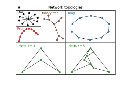
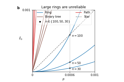
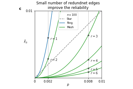
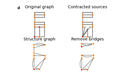
Figure 1: a shows different networks topologies with different redundancy($r$). b shows that large ring networks are unreliable and that radial networks are even more unreliable. The SAIDI index is plotted against the edge failure probabilities for different network structures (star, binary tree, path, and ring) and different numbers of nodes ($100,50,30$). c shows the optimal network near zero (edge failure probability) with $100$ nodes and various redundant edges ($r$ from $1$ to $6$). d Sparse graphs are easier to analyze through their structure graph. First, contact the sources into one node, such that all the neighbors of the old sources are the neighbors of the new source. Then, Turn each chain of nodes from degree two to one edge in the structure graph. Finally, Remove bridges. The nodes connecting to the bridges in these disconnected components can be considered the sources of these components.

Consider a graph $G=(V,E)$ with $n+1$ nodes, $m$ edges, and a designated source node $s\in V$. $p$ is the failure probability of all the edges in the network. We note that in the case of multiple sources, we can contract them into one source, as shown in figure 1.d. The SAIDI index is denoted as

$$\bar{F}_{G}=\frac{1}{n}F_{G}=\frac{1}{n}\sum_{v\in V}Pr_{G}(s\nleftrightarrow v)$$ (1)

is used to measure the reliability of the network.

Assume that $G$ is a radial(tree) network. In this scenario, the unreliability calculations are relatively simple. Each node that is $d$ distance away from the source works with a probability of $1-q^{d}$, where $q=1-p$ is the working probability. Therefore, the SAIDI index of the tree is

$$\bar{F}_{G} = 1-\mathbb{E}[q^{d}]=\mathbb{E}[d]\cdot p+o(p^{2})$$ (2)

This result implies that the most reliable trees are short and branched. As shown in figure 1.b, the star graph is the most reliable tree for all p values, while the path graph is the least.

We also calculate the explicit SAIDI index of a ring network. Each node works if at least one of its two disjoint paths to the source is working. Therefore, the SAIDI index for a ring network with one source and $n$ consumers is:

$$\bar{F}_{ring}(n) = \frac{1}{n}\sum_{k=1}^{n}\left(1-q^{k}\right)\left(1-q^{n+1-k}\right)$$

$$= 1+q^{n+1}-\frac{2}{n}\cdot\frac{q\left(1-q^{n}\right)}{p}$$

$$= \frac{1}{6}\left(n^{2}+3n+2\right)p^{2}+O\left(p^{3}\right)$$

This equation implies that despite the order of a ring network being two, large rings are unreliable because their $p^{2}$ coefficient is $O\left(n^{2}\right)$(fig 1.b). This phenomenon is a version of the birthday paradox: even though the probability of any specific edge pair failing is low, the number of such pairs is $O\left(n^{2}\right)$. Also, because each pair of edges, on average, disconnects $1/3$ of the nodes, the overall unreliability of the ring network is relatively high.

On the other hand, by reducing the length of the ring by dividing it into $k$ equally sized rings or by adding $k$ equally distributed sources to the ring, the SAIDI index is approximately $k^{2}$ times better.

$$\frac{\bar{F}_{rings}(n;k)}{\bar{F}_{ring}(n)}\approx\frac{\frac{n}{k}^{2}+3\frac{n}{k}+2}{n^{2}+3n+2}\overset{n\rightarrow\infty}{\longrightarrow}\frac{1}{k^{2}}$$ (4)

This equation demonstrates that a small change in the graph can lead to a significant improvement in reliability. The cases of unequal failure probabilities are discussed in the supplementary materials(supplementary A.5)

3 Analyzing sparse mesh networks

We can simplify the analysis of sparse mesh networks using various mathematical methods, including chain decomposition, decomposition of bridges, cut-set formula, and tree decomposition(supplementary D). The chain decomposition method[12] represents a path of $c$ nodes in a mesh network as a single edge with a failure probability of $1-q^{c+1}$, where $q$ is the probability of success(fig 1.d). This new graph is called the structure graph(or Distillation), its nodes are the hubs of the original graph, and its edges are called chains. The structure graph of the network $G$ is $S(G)$. If the number of redundant edges is small, the structure graph is also small and simple to analyze by, for example, using the ring-path formula(supplementary A.1). A bridge is an edge in the graph that, if removed, splits the network into two components. The bridge decomposition method involves analyzing each of those components independently(figure 1.d).

Finally, we use the cut-set formula to analyze the impact of each cut-set on the network reliability. A cut-set is a set of edges that separates the graph into multiple components, and a minimal cut-set is a cut-set that does not contain any other cut-sets. The set of all the minimal cut-sets of graph $G$ is $mcs_{G}$. We propose the risk index of a minimal cut set (RIC) to assess the effect of each minimal cut set on the SAIDI index. RIC of a minimal cut set $X$ is defined as the probability that $X$ fails and is connected to the source multiplied by the size of the disconnected component of $X$, represented as $D_{G}(X)$. Mathematically, RIC is expressed as:

$$R_{G}(X) = Pr_{G}\left(s\leftrightarrow X\wedge X\text{\,fail}\right)\cdot D_{G}(X)$$

$$= p^{\left|X\right|}\cdot D_{G}(X)+O\left(p^{|X|+1}\right)$$

Where $Pr_{G}(s\leftrightarrow X)$ is the probability that all the edges in $X$ are connected to the source. In essence, RIC represents the expected number of disconnected nodes resulting from the cut set failure. The SAIDI index of a graph is calculated using the risk index:

$$F_{G}=\sum_{X\in mcs_{G}}R_{G}(X)$$ (6)

Instead of analyzing all possible cut-sets in $G$, we can examine only those in the structure graph. Each minimal cut set $X^{\prime}\in E(S(G))$ disconnects $D_{G}(X^{\prime})$ nodes outside the chains of $X$. Also, the expected number of disconnected nodes from each chain $e^{\prime}\in X$ is approximate to $\frac{1}{2}\cdot c(e^{\prime})$, where $c(e^{\prime})$ is the length of the chain. Similarly, the failure probability of each chain is approximately $(c(e^{\prime})+1)p$.

As a result, an approximation of the cut-set risk in the structure graph is:

$$R_{G}(X^{\prime})=p^{\mid X^{\prime}|}\prod_{e^{\prime}\in X^{\prime}}\left(c(e^{\prime})+1\right)\left(D_{G}(X^{\prime})+\frac{1}{2}\sum_{e^{\prime}\in X^{\prime}}c(e^{\prime})\right)+O\left(p^{|X^{\prime}|+1}\right)$$ (7)

Another type of risk is the chain inter-risk. If the two nodes in the boundary of a chain are connected to the source, the chain becomes a ring. For each chain $e^{\prime}$, the chain inter-risk is

$$R_{G}(e^{\prime})=P_{2}(e^{\prime})\cdot F_{ring}(c(e^{\prime}))$$ (8)

Where $P_{2}(e^{\prime})$ is the probability that the two nodes on the boundary of the chain are connected to the source in the graph without the chain $e^{\prime}$. An approximation to the inter-chain risk is

$$R_{G}(e^{\prime}) = \frac{1}{6}p^{2}\left(c(e^{\prime})^{3}+3c(e^{\prime})^{2}+2c(e^{\prime})\right)+O\left(p^{3}\right)$$ (9)

The inter-risk is the expected number of disconnected nodes in the chain resulting from a cut set of nodes inside the chain. Combining the results above give us a formula for the SAIDI index in terms of the structure graph:

$$F_{G} = \sum_{X^{\prime}\in mcs_{S(G)}}R_{G}(X^{\prime})+\sum_{e^{\prime}\in E(S(G))}R_{G}(e^{\prime})$$ (10)

The complexity of the SAIDI calculation is due to the factors $Pr_{G}\left(s\leftrightarrow X\right),P_{2}(e^{\prime})$ in the risk formulas(3, 8). Fortunately, if $p$ and the chain’s length are small, we can settle for a 3rd-order approximation which is much easier to calculate. Additional information on computing 3rd-order approximations using the risk index and the approximation quality is discussed in the supplementary material(supplementary A.5).

We conclude that the SAIDI index is influenced by two types of cut sets: structural and inter-chain cut sets. The length of the chain influences inter-chain cut sets. The risk of a cut set in the structure graph is determined by equation 7, which considers the cut set’s order, the number of disconnected nodes and the multiplication of the cut set chain’s length. The sum of the SAIDI index of all the rings with the length of the graph chains is a lower bound to the network unreliability even if the structure graph is highly connected.

4 Construct the optimal graph

We have determined that the main risk factors of a graph are long chains, low-order structure graph cut sets, and the number of disconnected nodes resulting from these cut sets. The significance of each factor varies depending on the value of $p$ and the length of the chains. For small values of $p$ and short chains, the order and the number of minimal cut sets of the structure graph are the most critical factors. However, as $p$ and chain lengths increase, low-order cut sets with long chains that disconnect many nodes become more significant. For a large $p$, the most crucial factor is the proximity of the nodes to the source(supplementary C.2).

Based on these conclusions, we can characterize the optimal graph near zero as demonstrated in figure 2. The optimal network is the most reliable given a fixed number of nodes, redundant edges, and equal failure probability $p$. Firstly, the optimal is bridgeless to minimize the impact of low-order structure graph cut sets. Secondly, the optimal network should have equal-length chains to minimize the inter-chain risk, which is square in the length of the chain. A shorter chain length is a challenging task given a fixed number of redundant edges, but achievable by avoiding hubs with degrees greater than $3$. In fact, the optimal structure graph is $3$-regular, as a redundant edge between nodes of degree $2$ reduces the length of both chains, while a chain from a hub to a chain or from hub to hub reduces the length of one or zero chains, respectively. A graph with a $3$-regular structure graph, equal-length chains, and $k$-redundant edges contains $3(k-1)$ chains and therefore reduces the inter-chain risk by a factor of $9$ compared to the naive $k$-equal rings topology(supplementary C.3).

To further minimize the risk of three-order cut sets, the optimal network’s structure graph should also be $3$-connected. When the structure graph is $3$-connected, the only two-order risks present are the inter-chain risks. However, when the chains are long, or $p$ is large, there is a non-negligible probability of three-order cut sets in the structure graph(supplementary A.5). In this case, the optimal network should be super $3$-connected, meaning that the only three-order cut sets present are the trivial cut sets consisting of the edges connecting a node’s neighbors. Cubic super 3-connected networks always exist for any size[13]. Note that if third-order cut sets are not negligible due to long chains, the best solution is, if possible, reducing the chain’s length as it also reduces the chain inter-risk. The rules provided are enough to build a reliable graph because of the observation that a third-order approximation is adequate for small p, as shown in the supplementary subsection A.5. The results are fundamental because they hold for other reliability indices, such as the all-terminal reliability[11] and the pair-wise reliability(supplementary C.4).

Despite the simplicity of the model and the many assumptions we made, those design rules serve as the fundamental analytical rules of reliable network planning. These rules are easy to interpret and can be identified at a glance without the need for complicated numeric simulations. However, to make real-world decisions, other essential variables must be considered, such as the cost of each edge, the weight of each node, and the diversity of the edge failure probabilities. For example, in most cases, the optimal network does not have an equal chain length due to geometrical considerations(figure 4). To give more accurate results, the risk approximation formulas presented earlier are helpful tools, as discussed in the next section.

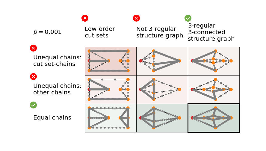
Figure 2: The optimal network has a $3$-regular and super $3$-connected structure with equal-length chains. The table above compares network topologies with $120$ nodes and $124$ edges, with color indicating the SAIDI index ($p=0.001$). The columns show different structure graphs, and the rows show different chain lengths. Although covering all network topologies is impossible, we can see that unequal chains reduce network reliability and that, if they exist, they should not be on the edges of low-order structure graphs. Also, if the structure graph is not $3$-regular, the number of chains is lower, causing longer and less reliable chains.

5 Improve existing network

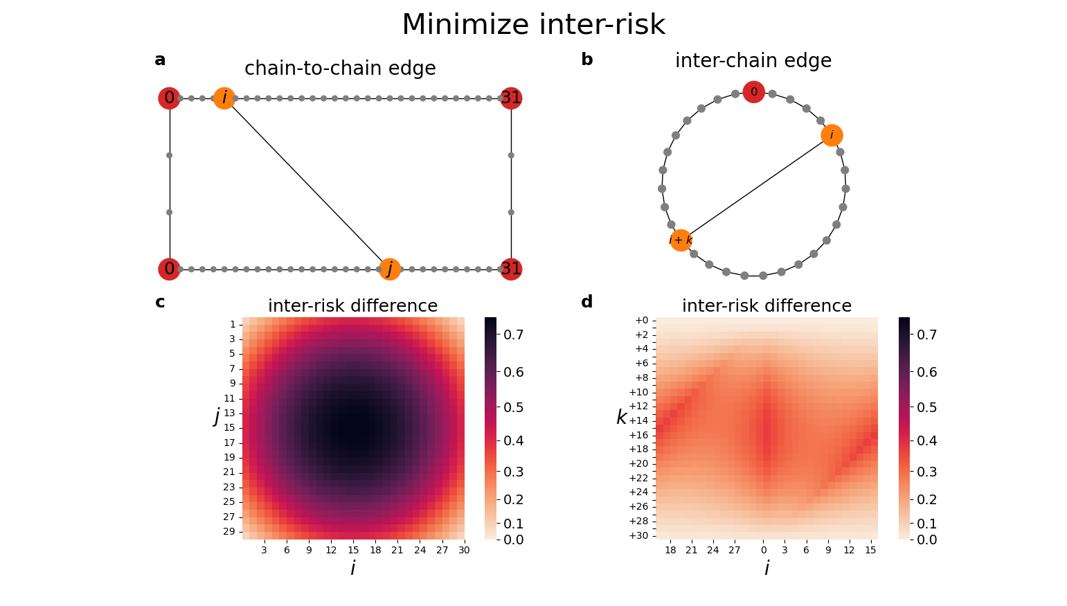
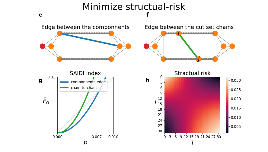
Figure 3: The figure shows the effect of adding a new edge on inter and structural risks. The first row demonstrates a chain-to-chain edge(a) and inter-chain edge(b). c present the inter-risk difference of the chain-to-chain edge from node $i$ to $j$ (as presented in a) d presents the inter-risk of an inter-chain edge from node $i$ to $i+k$, clockwise(as presented in b). We observed that chain-to-chain edges have a greater inter-risk difference. The optimal chain-to-chain edges should be positioned close to the center of each chain, and the best inter-chain edge should have a length equal to half a chain and start as close as possible to the source. If $i=0$ in both edges type, the edge is a hub-to-chain edge. Minimizing the structural risk of a minimal cut set is possible by adding an edge between the two components separated by the cut set(e) or by adding an edge that touches at least one of the cut set chains(f). g compares the SAIDI index after adding each edge kind and demonstrates that adding an edge between the cut set components is more effective. Finally, h shows the SAIDI index after adding the edge $(i,j)$ as depicted in figure f. It follows that the optimal edge has one end in one of the components and the other end in the other component.

We can use the risk difference to measure the effectiveness of adding a new edge to an existing network. The risk difference is between the risk of some cut set $X$ before and after adding a new edge $e$.

$$\Delta R_{G}(X;e)=R_{G}(X)-R_{G\cup\{e\}}(X)$$ (11)

By summing the risk difference for each edge and the predefined cost of it, we can decide which new edge is the most beneficial. You can find exact formulas for the risk difference of any edge in the general model in supplementary B. The effect of adding new edges to an existing network is limited because it creates chains from length 1. Therefore, good preplanning is preferred, as demonstrated in figures 4 and 5.

It is possible to add four different types of edges to a network: chain-to-chain, inter-chain, hub-to-chain, and hub-to-hub connections. Adding a chain-to-chain edge is the most effective in reducing inter-risk, as it transforms a pair of rings into four rings. Hub-to-chain edge is A specific case of chain-to-chain, which is less effective as it only affects one chain. An inter-chain edge is also less effective because it turns a ring into three rings but produces another order two structural cut set. Lastly, a hub-to-hub edge does not affect inter-risk at all. Figure 3(a-d) compares the effect of each edge type on the inter-risk. It follows that the optimal chain-to-chain edge touches the middle of each chain, and the optimal hub-to-chain and inter-chain edges are from the end to the middle of the chain, dividing the chain into two equal rings. The optimal chain-to-chain edge is approximately $2$ times better than the other edge types in reducing inter-risk(supplementary B.1).

There are two options to reduce the structural risk of a minimal cut set(figure 3(e-h)): adding an edge between the two components separated by the minimal cut set or adding an edge that divides one or two of the minimal cut set chains. The first option is the most effective in reducing structural risk because it raises the order of the cut set. However, the second option only minimizes the coefficient of the polynom and not its order. The closer one side of the new edge is to the source component and the other side to the disconnected component, the bigger the risk difference, as shown in figure 3. For this reason, chain-to-chain edges are also more effective than inter-chain edges in reducing structural risk.

6 real-world analysis

We demonstrate the main ideas of our research in two examples: the Baran & Wu system and grid networks. The Baran & Wu system is a synthetic distribution network[14]. The system has one source, 32 loads, and 37 edges(figure4.b). Despite its high redundancy and cost, the network is unreliable due to a bridge that disconnects the entire network. Figure 4 shows several versions of the same nodes. In each version, we display the ratio of the network’s length and SAIDI index compared to the basic ring network. Furthermore, we present the top $5$ risks for each example and use them to improve the network. Using the risk analysis, we managed to construct more cost-effective versions of this network while keeping the budget at a $10$ extra length than the ring version and improving the network reliability up to $8.83$ times more than the ring network. However, due to the sparsity of the network nodes, it is hard to further improve the network without using high-cost edges.

The second example is a $7\times n$ grid with sources in the left upper and the right bottom corners(figure 5). This example is important because the grid is a common topology among cities. A basic approach is filling the top and bottom rows, creating chains with $n$ nodes. A naive improvement for this topology is a grid configuration with a middle row that divides each ring into two equal rings. However, this design is not agreed with the design rule of making hubs with a degree of $3$. To address this problem, we separated the middle row into a $1/3,2/3$ configuration that divided the middle chain into three almost equal chains and the outer chains into two nearly equal chains. This new configuration improves the SAIDI ratio by a factor of $6$, which is $1.54$ times better than the naive middle-row configuration even though the number of nodes is very high. Also, by defining the number of redundant edges between every two consecutive chains, we can use a dynamic programming algorithm to find the optimal edge configuration(supplementary E.1). Figure 5 presents the optimal and the nonoptimal configurations. The downside of those configurations is that the east-west chains are from length $1$.

Finally, we analyze three real distribution networks from the Atlantic City website. Distribution networks tend to traverse major roads[15]. Therefore, we illustrate that by adding a relatively small number of redundant edges based on roads, we can transform the ring-like topologies into sparse mesh topologies, which improved the SAIDI ratio by a factor of $27.12$ to $3.14$ for $p=0.0001$. The data is taken from the electrical vehicle load capacity map on March 2023. Although the map is not necessarily accurate, the data demonstrate a real-world distribution network. More technical details of the analysis are in the supplementary E.2.

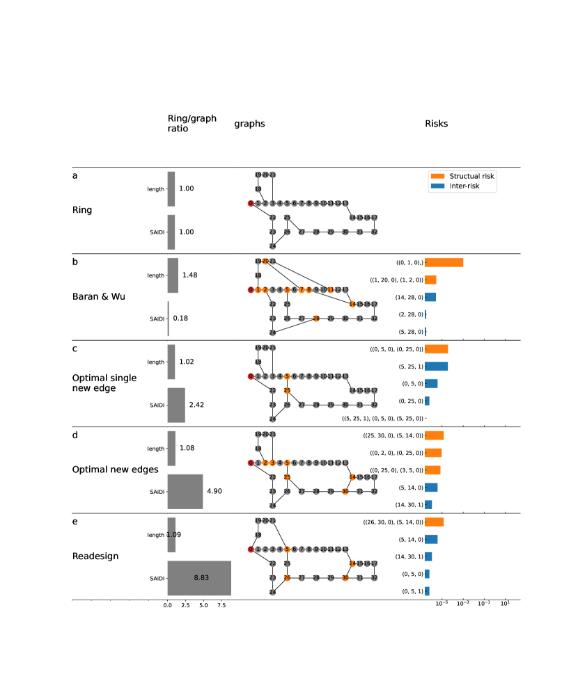
Figure 4: Improve the Baran & Wu system. The first row represents the original test case with high density but low reliability. The second row introduces a ring approach, while subsequent rows show further enhancements. Comparisons of the mesh networks to the ring configuration are made based on edge lengths, SAIDI(column 2), and identifying the top 5 risks(last column). The last row demonstrates that designing a network from scratch proves more effective than adding edges to an existing network.

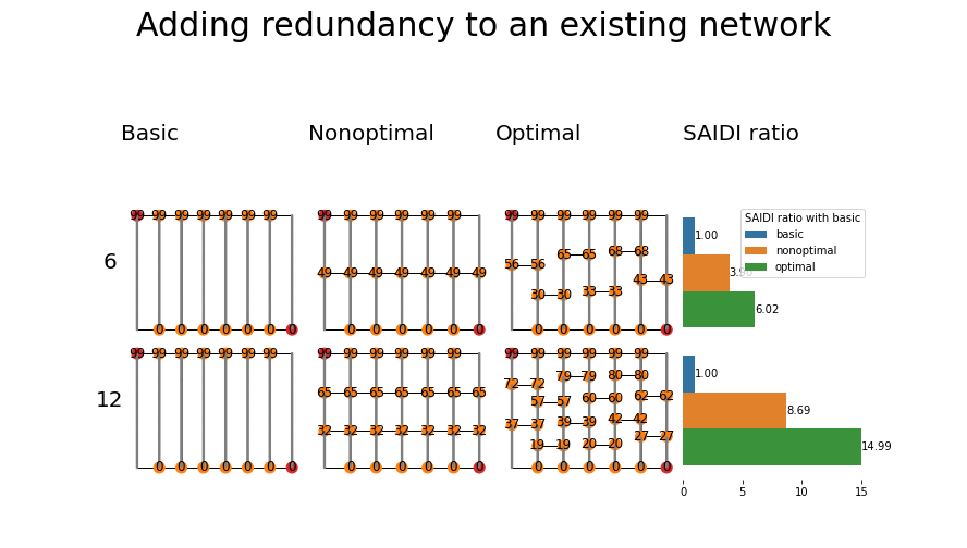
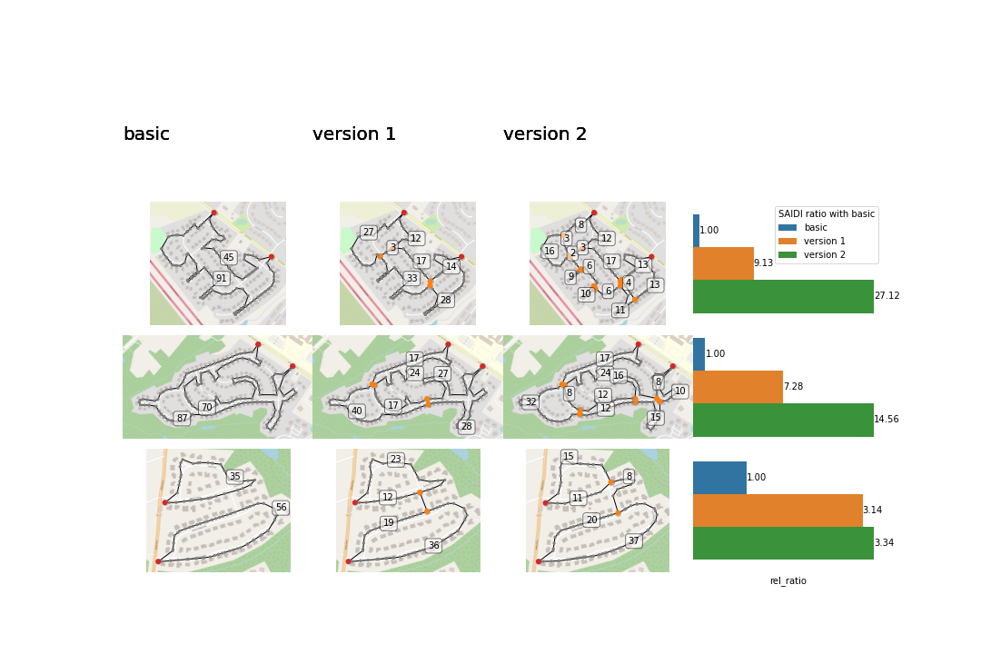
Figure 5: Adding redundant edges for existing networks. The upper figure presents a common $100X7$ grid topology with vertical and horizontal edges in the upper and bottom rows. In each row of the figure, we add redundant edges as presented in the second column(nonoptimal) and the same amount of redundant edges with a more equal-chains topology in the third column(optimal). The right column shows the SAIDI ratio of the basic network to the nonoptimal network(in orange) and the optimal network(in green). By creating hubs with three neighbors, we get more chains and improve the grid’s reliability. Also, we observed that a small number of new edges significantly improved the reliability. The lower figure shows real ring networks(on the left column) and two versions of modifications to the network. The right column compares the SAIDI ratio of those versions to the original network. The floating numbers represent the number of nodes in each chain. By following the design rules, we significantly improved the networks with a relatively small amount of redundant edges.

Appendix A Exact analysis of the general model

A.1 SAIDI computation

This section provides a formula for the SAIDI index of various topologies in the general weight-probabilities model. The SAIDI index of a network $G$ is calculated through its minimal cut sets risk(proposition 1).

$$F_{G}=\sum_{X\in mcs_{G}}R_{G}(X)=\sum_{X\in mcs_{G}}Pr_{G}\left(s\leftrightarrow X\wedge X\text{\,fail}\right)\cdot D_{G}(X)$$ (12)

To calculate $Pr_{G}(s\leftrightarrow X\wedge X\text{\,fail})$, we focuses on $cc(X)$ - the connected component of $s$ after the removal of $X$ and use the inclusion-exclusion principle

$$Pr_{G}(s\leftrightarrow X\wedge X\text{\,fail}) = Pr_{G}(X)\cdot\sum_{\chi\subseteq mcs_{cc(X)}(X)}(-1)^{|\chi|-1}\cdot Pr_{G}\left(\bigcup_{A\in\chi}A\right)$$ (13)

Where $mcs_{cc(X)}(X)$ is the set of all minimal cut sets of $cc(X)$ that disconnect $X$ from the source. This formula complexity is $O\left(2^{\left|mcs_{cc(X)}(X)\right|}\right)$. Fortunately, if the probabilities $p_{e}$ are sufficiently small, we can ignore the probability of high-order cut sets. Subsection A.5 contains the specific details of this approximation. As mentioned in the main article, we can simplify the SAIDI computations in a sparse network by enumerating only the minimal cut sets of the structure graph.

The ring-path formula is another method to calculate the SAIDI index of a sparse network based on its structure graph. We can determine the expected number of disconnected nodes from a specific chain $(u,v)$ in the structure graph by considering the different scenarios that can occur if we remove the chain, as presented in figure 6. For example, assume that the chain contains $c$ nodes. If both nodes $u$ and $v$ are disconnected, the entire chain is disconnected, resulting in $f_{0}=c$ disconnected nodes. If only one of them is connected, the chain becomes a path with $c$ nodes, resulting in $f_{1}=F_{path}(c)$ disconnected nodes on average. Finally, if both nodes are connected, the chain becomes a ring with $c$ nodes, resulting in $f_{2}=F_{ring}(c)$ disconnected nodes on average. We can use the probabilities of each of these cases $P_{0}(e^{\prime}),P_{1}(e^{\prime}),P_{2}(e^{\prime})$ to calculate the ring-path formula:

$$F_{G} = \sum_{e^{\prime}\in E(S(G))}\sum_{i=0}^{2}f_{i}(e^{\prime})\cdot P_{i}(e^{\prime})+F_{S(G)}$$

$$= \sum_{e^{\prime}\in E(S(G))}c(e^{\prime})\cdot P_{0}(e^{\prime})+F_{path}(e^{\prime})\cdot P_{1}(e^{\prime})+F_{ring}(c(e^{\prime}))\cdot P_{2}(e^{\prime})+F_{S(G)}$$

where $S(G)$ is the structure graph of $G$. Additionally, in the general weight-probabilities model, the chains are not symmetric. Hence, two types of $P_{1}$ events exist. Each connected node in the boundary of the chain creates a path with a different source. In this scenario, we can use the more general partitions formula. For a set of nodes $X\subseteq V(G)$, denote $\pi(X)$ as the set of all the partitions of $X\cup\{s\}$. Assume that the graph is partition into two subgrphs $A_{1}\cup A_{2}=G$, and denote $X=A_{1}\cap A_{2}$. We can split the probability space of $G/A_{i}$ to an equivalence class defined by the connected components of $X\cup\{s\}$. Given a specific partition in $G/A_{i}$, we can contract all the nodes in $A_{i}$ that are in the same partition component to one node. Then, by the law of total probability:

$$F_{G}=\sum_{i=1}^{2}\sum_{\chi\in\pi(A_{1}\cap A_{2})}Pr_{A_{i}^{c}}(\chi)\cdot F_{A_{i}\mid\chi}$$ (15)

Where $A_{i}\mid\chi$ is the graph $A_{i}$ after contracting each component in $\chi$ to one node(figure 7). As a private case, the ring-path formula in the general model is

$$F_{G}=\sum_{(u,v)\in E(S(G))}\sum_{\chi\in\pi(\{u,v\})}Pr_{G/(u,v)}(\chi)\cdot F_{C(u,v)\mid\chi}+F_{S(G)}$$ (16)

Where $C(u,v)$ is the chain from $u$ to $v$.

This article showcases several applications of the partition formula. One of its applications is a fast algorithm that can compute the network’s reliability using tree decomposition(subsection D.1). When combined with the ring-path formula, this algorithm can also calculate the SAIDI index of a network even faster. Another application of the partition formula is the modularity of network planning. For instance, if we have a neighborhood $A\in G,$ we can quickly identify the impact of changes made inside the neighborhood, such as adding or removing edges, as we only need to identify those changes on the indexes $F_{G\mid\chi}$ for $\chi\in\pi(A\cap A^{c})$. For example, in subsection E.1, we design reliable grids using this formula.

A private case of the partitions formula is bridge decomposition[12]. A bridge is an edge $e=(u,v)$ that, if removed, splits a set of nodes $X$ from the source. For example, suppose that $u$ is a member of $X$ and mark the subgraph of $X$ in $G$ with $u$ as the source node as $G_{X}$, then for any other node $w$ in $X$, the probability that $w$ is connected to the source is

$$Pr_{G}(s\leftrightarrow w)=Pr_{G}(s\leftrightarrow v)\cdot p_{e}\cdot Pr_{G_{X}}(u\leftrightarrow w)$$ (17)

This means that by adding the weight $1-p_{e}\cdot F_{G_{X}}$ to the node $u$, we can remove $X$ from $G$, thereby reducing the size of the graph and ensuring that there are no bridges in it.

Finally, we use the risk sum formula to compute the SAIDI index of the network.

Proposition 1 (The risk formula).

For a network $G$, $F_{G}$ is the sum of the risks associated with all minimal cut sets:

$$F_{G}=\sum_{X\in mcs_{G}}R_{G}(X)$$ (18)

Proof.

Let $v$ be a node in the network. We denote the set of all minimal cut sets that disconnect $v$ from the source $s$ as $mcs_{G}(s,v)$. If $v$ is disconnected from the source, there is a unique minimal cut set in $mcs_{G}(s,v)$ that fails, and all its edges are reachable from the source. This minimal cut set is the set of edges between the connected component of $v$ and the source component.

The probability space can be split into disjoint sets by the unique reachable minimal cut set in $mcs_{G}(s,v)$. The probability that $X$ is the reachable failing cut set is $Pr_{G}(s\leftrightarrow X)\cdot Pr_{G}(X)$. Summing over all the nodes of the network gives us the desired formula. Therefore, we can express the total risk of the network as the sum of the risks associated with all minimal cut sets in $G$. ∎

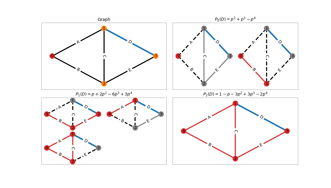
Figure 6: The ring-path formula. The probability that $i$ nodes from the boundary of chain $D$, after its removal from the structure graph, are connected to the source (denoted as $P_{i}(D)$) can be calculated by considering all the minimal cut sets in $G/\{D\}$ and applying the inclusion-exclusion principle. The graph above presents the minimal cut sets for each $i$, with node $0$ representing the source. Edges represented as dashes indicate disconnections, red nodes and edges show connections to the source, and grey elements depict disconnections.

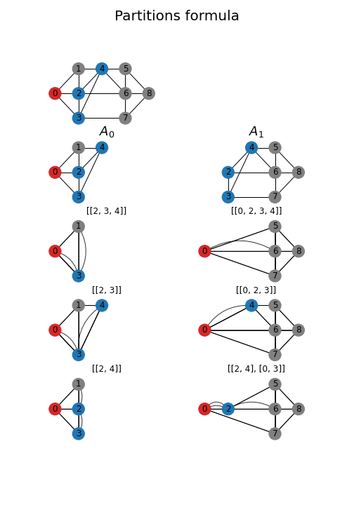
Figure 7: The partitions formula. A graph is divided into two subgraphs, and the partitions formula is used to compute the SAIDI index. The graph separates into two subgraphs $A_{0},A_{1}$. the intersection nodes are $X=\{2,3,4\}$(in blue). To calculate the reliability of the nodes in $A_{i}$, we compute the probability for each partition of the nodes in $X\cup\{s\}$ in the graph $A_{i}^{c}$ that the partition is the connected components of the nodes in $X$ in the graph $A_{i}^{c}$. We contract all the nodes in the same partition components for each such partition.

A.2 Radial networks

Here we present the analytical analysis of the radial networks’ reliability in the general model. The SAIDI analysis of the general tree is quite simple. Let the set of edges in the unique path between $s,v$ be $path(s,v)$. Note that

$$Pr_{T}(s\nleftrightarrow v)=1-\prod_{e\in path(s,v)}q_{e}$$ (19)

and hence, the SAIDI index of a tree $T$ is

$$F_{T}=\sum_{v\in V(T)}\left(1-\prod_{e\in path(s,v)}q_{e}\right)\cdot w_{v}$$ (20)

Where $\omega_{v}$ is the weight of the node $v$.

To calculate the risk of each edge, denote the total weight of disconnected nodes resulting from the failure of an edge $e$ as $D_{T}(e)$. The risk of an edge $e$ is

$$\begin{cases}R_{T}(e)=\left(\prod_{e^{\prime}\in path(s,e)}q_{e^{\prime}}\right)\cdot p_{e}\cdot D_{T}(e)\\ F_{T}=\sum_{e\in E(T)}R_{T}(e)\end{cases}$$ (21)

By set $q_{e^{\prime}}=1-p_{e^{\prime}}$ in 21, it follows that the polynom coefficients are

$$F_{T} = \sum_{e\in E(T)}\sum_{J\subseteq path(s,e)}(-1)^{|J|}D_{T}(e)\left(p_{e}\prod_{e^{\prime}\in J}p_{e^{\prime}}\right)$$ (22)

And that the first-order approximation is

$$F_{T} \approx \sum_{e\in E(T)}p_{e}\cdot D_{T}(e)$$ (23)

As a private case, the SAIDI index of a tree in the equal probabilities-weights model is

$$F_{T} = \sum_{k=1}^{n}(-1)^{k-1}\left(\sum_{a=k}^{n}d(a)\cdot{\binom{a}{k}}\right)p^{k}$$ (24)

Where $d(a)$ is the number of the nodes at a distance $a$ from the source. By set $d(a)=1$ and using the hockey Stick Identity[16] we get The SAIDI index of a path

$$F_{path}(n)=\sum_{k=1}^{n}(-1)^{k-1}{\binom{n+1}{k+1}}p^{k}$$ (25)

A.3 Ring networks

To calculate the SAIDI index of a general ring, we observed that each ring node connects in two disjoint paths to the source(figure 11)

$$F_{ring}=\sum_{v=1}^{n}\left(1-\prod_{i=1}^{v}q_{i}\right)\left(1-\prod_{i=v+1}^{n+1}q_{i}\right)\cdot w_{v}$$ (26)

And in the risks method, each minimal cut set is a pair of edges $\{i,j\}$

$$R_{ring}(\{i,j\}) = \prod_{k=1}^{i}q_{k}\prod_{k=j+1}^{n+1}q_{k}\cdot p_{i}p_{j}\cdot\sum_{k=i}^{j}w_{k}$$

$$= \left(\prod_{k=1}^{n+1}q_{k}\right)\left(p_{i}p_{j}\right)\left(\frac{\sum_{k=i}^{j}w_{k}}{\prod_{k=i}^{j}p_{k}}\right)$$

We can see that a ring cut set risk depends on the failure probability of the cut set($p_{i}p_{j}$), by $D_{ring}(\{i,j\})=\sum_{k=i}^{j}w_{k}$ , and by the probabilities product of the disconnected path($\prod_{k=i}^{j}p_{k}$). Another insight is that in the equal weight-probabilities model

$$R_{ring}(\{i,j\})<R_{ring}(\{i^{\prime},j^{\prime}\})$$ (28)

For $i^{\prime}<i,j^{\prime}>j$ and $i<j$. However, unlike the equal probabilities model, where the maximal risk is of the two edges that are connected to the source, in the general model, any cut set can have the maximal risk for the appropriate parameters. The SAIDI index of the ring with $n$ consumers is computed in $O(n)$ using a dynamic programming approach.

In the equal weights-probabilities model

$$F_{ring}(n)=\sum_{k=2}^{n+1}(-1)^{k}(k-1)\binom{n+2}{k+1}p^{k}$$ (29)

A.4 Structural risk

The exact calculation of the risk difference after adding a new edge is hard to calculate. However, there are some methods to approximate this risk difference relatively quickly. We present the exact risk difference of each kind and, in the approximation section, provide the proper approximations.

The structural risk of a structural graph cut set defines as

$$R_{G}(X^{\prime}) = Pr_{S(G)/X^{\prime}}(s\leftrightarrow X^{\prime})\left(Pr_{S(G)}(X^{\prime})\cdot D_{G}(X^{\prime})+\sum_{C\in X}Pr_{S(G)}(X^{\prime}/C)\cdot F_{path}(C)\right)$$ (30)

$$= Pr_{S(G)/X^{\prime}}\left(s\leftrightarrow X^{\prime}\right)\cdot Pr_{S(G)}\left(X^{\prime}\right)\left(D_{G}(X^{\prime})+\sum_{C\in X}\frac{F_{path}(C)}{Pr_{G}(C)}\right)$$

The probability $Pr_{S(G)}(X^{\prime})=\prod_{C\in X^{\prime}}\left(1-\prod_{e\in C}q_{e}\right)$. $F_{path}(C)$ calculate using equation 20 or 22. Subsection D.1 explains how to calculate the probability $Pr_{S(G)}(s\leftrightarrow X^{\prime})$. Although, calculating the precise value of $Pr_{S(G)}(s\leftrightarrow X^{\prime})$ is a hard task; if we examine only cut sets from orders less than $k$, then we calculate the reaching probability up to order $k-\left|X\right|$.

We can approximate the structural risk using the approximations introduced in section A.2. For example, in the equal probabilities-weights model, the most basic approximation is

$$R_{G}(X^{\prime})=p^{\mid X^{\prime}|}\prod_{e^{\prime}\in X^{\prime}}\left(c(e^{\prime})+1\right)\left(D_{G}(X^{\prime})+\frac{1}{2}\sum_{e^{\prime}\in X^{\prime}}c(e^{\prime})\right)+o\left(p^{|X^{\prime}|+1}\right)$$ (31)

A.5 Approximations

We aim to determine the minimum order required to achieve a satisfactory approximation. The accurate computation of SAIDI is not feasible for graphs with many edges[17]. Our primary focus is identifying weak points in the network and determining which new edges to add, which involves analyzing all the lower-order cut sets. However, the calculations are inefficient due to a large number of minimal cut sets and their intersections in the inclusion-exclusion principle. However, if $p$ is small, the number of concurrent failures is relatively low, allowing us to examine only lower-order cut sets. Additionally, not all simultaneous failures lead to network breakdown, so that lower-order cut sets can approximate reliable graphs more easily. The critical question is, what minimum order is required to achieve a satisfactory approximation? To answer this question, we first examine the approximations of fundamental components such as ring, chain, and structural risk and then analyze the approximation of several graphs.

Figure 8 presents the approximation quality of fundamental network components. Although the precise calculation of these components is straightforward, their exact evaluation is unnecessary. For each order of approximation, the figure displays the minimum p with an error deviation of at least $\epsilon=0.0001$ from the actual value ($p_{0}$) as a function of chain length($c$). If the approximation order is smaller than the minimum non-zero coefficient, the approximation is zero, indicating that the risk of the component can be ignored. The figure indicates that the ring and chain failure components are relatively accurate for orders $2$ or $3$.

We use equal chain configurations to estimate the approximation quality of structural risks. This choice is based on the observation that equal chains represent the most unreliable configuration regarding structural risk, as the failure probability is the product of each chain’s failure probability (it is worth noting that equal chains aim to minimize inter-risks). Consequently, estimating the error in the equal chain’s configuration provides an upper bound for the error in structural risk when dealing with unequal chains but an equal number of nodes. However, the approximation error increases when a significant number of nodes become disconnected (denoted as $D_{G}(X)$). This implies that even 5th-order structural cut sets cannot be disregarded if the number of disconnected nodes is sufficiently large. Figure 8 illustrates a 2nd-order and 3rd-order structural cut set using equal chains of length $c$ that disconnect $d=100$ nodes.

Figure 9 demonstrates that a second or third order of approximation is adequate for small $p$. The figure examines three different topologies, one with a second-order structural cut set, one with a significant four-order cut set, and one with a super $3$-connected structure graph. The graphs have equal-length chains, but a more heterogeneous configuration results in an even more accurate approximation. The vertical lines represent $p_{0}$, the minimum $p$ with an approximation error of at least $\epsilon=0.0001$. In summary, a second or third-order approximation is sufficient for small $p$, even for networks with many nodes. Although very unreliable network approximations may be inaccurate, they are rare in practice because of their ineffectiveness.

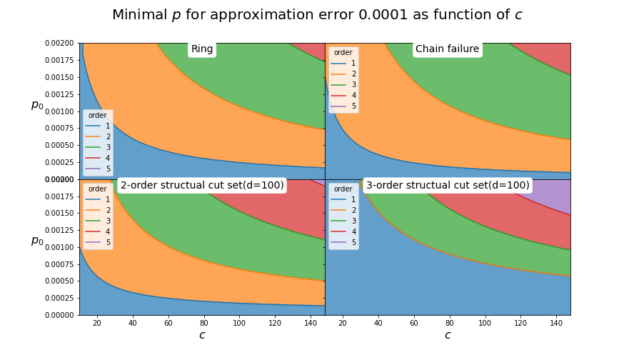
Figure 8: The figure displays the minimum order of approximation required to achieve an error deviation of at least $0.0001$ from the actual value ($p_{0}$) for each fundamental network component. The x-axis represents the length of the chains, while the y-axis represents $p_{0}$. The structural cut sets in the figure result in $100$ disconnected nodes.

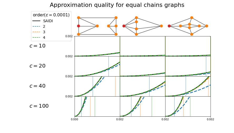
Figure 9: The figure illustrates the quality of low-order approximation for several structured graphs with different equal-length chains. The vertical lines in the figure represent $p_{0}$, which is the minimum value of $p$ required for a satisfied approximation with an error deviation of at least $0.0001$.

A.6 Inter-risk

Calculating a third-order approximation of the inter-risk for a chain in the structure graph is straightforward. The challenge lies in calculating $P_{2}(e^{\prime})$. Fortunately, using only the first order of $P_{2}(e^{\prime})$ provides a good approximation because the SAIDI polynomial of a ring is $O(p^{2})$, and an order three approximation is accurate enough for SAIDI calculations. To compute the inter-risk of an edge $e^{\prime}$ in the structure graph G, use the following formula:

$$R_{G}(e^{\prime})=\left(1-\sum_{e\in B_{G}(e^{\prime})}p_{e}\right)\cdot F_{ring}(e^{\prime})$$ (32)

Here, $B_{G}(e^{\prime})$ is the set of all bridges in the graph that disconnect $e^{\prime}$ from the source. In the equal probabilities-weights model:

$$R_{G}(e^{\prime})=\frac{1}{6}\left(1-\left(\sum_{C\in B_{S(G)}(e^{\prime})}(c(e^{\prime})+1)\right)p\right)\cdot\left(c(e^{\prime})^{3}+3c(e^{\prime})^{2}+2c(e^{\prime})\right)$$ (33)

Appendix B Risk difference analysis

In this section, we provide the formulas for calculating the risk difference that results from adding a new edge. Throughout this section, we assume that we have identified all the minimal cut sets of the network up to the desired order. More details about the algorithm for finding these cut sets are in subsection D.2.

To find the risk difference of a new edge $e$ we only need to calculate $R_{G\backslash e}$. $G\backslash e$ is the network $G$ after contracting the nodes of $e$. From the definition of risk difference $\Delta R_{G}(X;e)=R_{G}(X)-R_{G\cup\{e\}}(X)=R_{G}(X)-p_{e}R_{G}(X)-q_{e}R_{G\backslash e}(X)$ and hence

$$\Delta R_{G}(X;e)=q_{e}\left(R_{G}(X)-R_{G\backslash e}(X)\right)$$ (34)

The purpose of this risk difference analysis is twofold. Firstly, we aim to understand the impact of a new edge on the graph. For example, a chain-to-chain edge is typically more efficient than an inter-chain edge. Secondly, we aim to efficiently approximate the impact of the new edge on the risk difference. There are four types of new edges: chain-to-chain, inter-chain, hub-to-chain, and hub-to-hub. We begin by analyzing the inter-risk difference of all new edge types and then analyzing the structural risk difference.

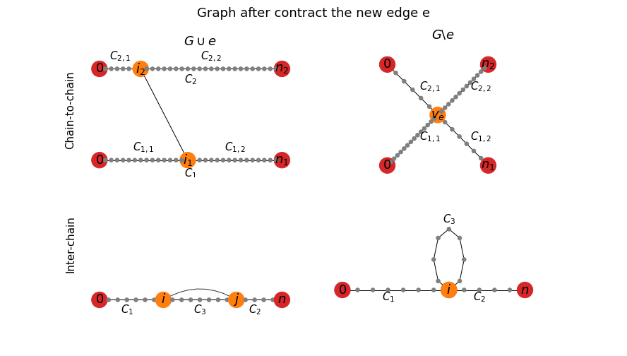
Figure 10: Adding a chain-to-chain and inter-chain new edge. The left column represents the new edge and the right column represents the graph after the contraction of the edge.

B.1 Inter-risk difference

We only need to analyze chain-to-chain and inter-chain edges to understand the inter-risk difference, as hub is the zero node of a chain. The inter-risk formula is $R_{G}(C)=P_{2}(C)\cdot F_{ring}(C)$. The hub-to-hub edge can affect only $P_{2}(C)$.

Chain-to-chain

Assume that there are two chains $C_{1},C_{2}$, and that we add an edge $e$ between the $i_{1}$ node on the chain $C_{1}$, and the $i_{2}$ node on the chain $C_{2}$(figure 10). The new edge is dividing each of the chains $C_{k}$ into two smaller chains $C_{k,1},C_{k,2}$. After contracting the edge $e$, the chains $C_{1}$ and $C_{2}$ are turning into star network subgraphs with the node $v_{e}$ in the middle(figure 10). Note that the contraction of the edge does not change the value of $P_{2}(C_{k})$.

$$R_{G\backslash e}(C_{k}) = P_{2}(C_{k})[Pr_{G/C_{k}}\left(s\leftrightarrow v_{e}\mid P_{2}(C_{k})=1\right)\left(F_{ring}(C_{k,1})+F_{ring}(C_{k,2})\right)$$ (35)

$$+ \left(1-Pr_{G/C_{k}}\left(s\leftrightarrow v_{e}\mid P_{2}(C_{k})=1\right)\right)\left(F_{ring}(C_{k})\right)]$$

Which is the risk given that $v_{e}$ is connected to the source in $G\backslash C_{k}$ plus the risk given the complementary event. From here,

$$R_{G\backslash e}(C_{k}) = P_{2}(C_{k})Pr_{G/C_{k}}\left(s\leftrightarrow v_{e}\mid P_{2}(C_{k})=1\right)\left(F_{ring}(C_{k,1})+F_{ring}(C_{k,2})-F_{ring}(C_{k})\right)$$ (36)

$$+ P_{2}(C_{k})F_{ring}(C_{k})$$

Therefore,

$$\Delta R_{G}(C_{k};e) = q_{e}\cdot Pr_{G/C_{k}}\left(s\leftrightarrow v_{e}\wedge P_{2}(C_{k})=1\right)\cdot\left(F_{ring}(C_{k})-F_{ring}(C_{k,1})-F_{ring}(C_{k,2})\right)$$ (37)

$$\overset{\text{order\,2}}{\approx} F_{ring}(C_{k})-F_{ring}(C_{k,1})-F_{ring}(C_{k,2})$$

We can infer some insights about the optimal new edge from the equation above. The position of the edge in $C_{2}$ should maximize the probability $Pr_{G/C_{1}}\left(s\leftrightarrow v_{e}\wedge P_{2}(C_{1})=1\right)$ to minimize the inter-risk of $C_{1}$, which imply that the edge should be close to the boundary of $C_{2}$. On the other hand, by adding the new edge, we remove minimal cut sets that are edges pairs from the opposite sides of the new edge, which imply that the optimal new edge is closer to the middle of $C_{1}$ in relative equal weights and probabilities (Although this can change in a heterogeneous chain). Equation A.3 explains the causes of high-risk minimal cut sets in a chain and can help analyze the optimal new edge’s location. For example, the optimal new edge in equal-length and homogeneous chains is from the middle of each chain.

Inter-chain

Assume that there is a chain $C$, and that we add an edge $e$ between the $i$ and the $j$ node of the chain(figure 10). After the contracting of the edge $e$, the chain transforms into a smaller chain $C_{1}\cup C_{2}$ with a self-loop in the $i$ node denoted as $C_{3}$. The risk of the chain after the contraction of $e$ i

$$R_{G\backslash e}(C)=P_{2}(C)\cdot\left[F_{ring}(C_{1}\cup C_{2})+p_{C1}p_{C2}\left(w(C_{3})-F_{ring}(C_{3})\right)+F_{ring}(C_{3})\right]$$ (38)

Where $p_{C_{k}}$ is the failure probability of the chain $C_{k}$, and $w(C_{3})$ is the total weight of $C_{3}$.

$$\Delta R_{G}(C;e) = q_{e}\cdot P_{2}(C)\cdot\left[F_{ring}(C)-F_{ring}(C_{1}\cup C_{2})-F_{ring}(C_{3})-p_{C1}p_{C2}\left(w(C_{3})-F_{ring}(C_{3})\right)\right]$$ (39)

$$\overset{\text{order\,2}}{\approx} F_{ring}(C)-F_{ring}(C_{1}\cup C_{2})-F_{ring}(C_{3})-p_{C1}p_{C2}w(C_{3})$$

In the equal probabilities-weights model, the optimal chain-to-chain edge is approximately two times better than the other edge types in reducing inter-risk. Suppose there are two chains with $n$ nodes. The optimal chain-to-chain edge divides two chains into two chains, but the optimal inter-chain edge divides only one chain into two chains.

B.2 Structural risk

The hub-to-chain is a private case of chain-to-chain or inter-chain, even in the structural risk scenario. To simplify the calculations we introduce the notation $\rho(X,D)$ for a set of chains $X$ and a number $D$

$$\rho(X,D)=Pr_{S(G)}(X)\cdot D+\sum_{C\in X}Pr_{S(G)}(X/C)\cdot F_{path}(C)$$ (40)

And the structural risk formula transform to $R_{G}(X)=Pr_{G/X}(s\leftrightarrow X)\cdot\rho(X,D_{G}(X))$

Chain-to-chain

Suppose there is a new edge between two of the chains $C_{1}$ and $C_{2}$ of the structural cut set similar to figure 10. Denote $X^{\prime}=X/(C_{1}\cup C_{2})$. After contracting the new edge, the structural cut set transforms into two structural cut sets: $X_{1}=X^{\prime}\cup\{C_{1,1}\cup C_{2,1}\}$ and $X_{2}=X^{\prime}\cup\{C_{1,2},C_{2,2}\}$. The first cut set disconnects a weight of $D_{G}(X_{1})=D_{G}(X)+w(C_{1,2}\cup C_{2,2})$, and the second cut set disconnects a weight of $D_{G}(X)$.

$$R_{G\backslash e}(X)=Pr_{G/X}(s\leftrightarrow X)\cdot Pr_{G}(X^{\prime})\cdot\left(\rho(X_{1},D_{G}(X_{1}))+\rho(X_{2},D_{G}(X))\cdot(1-p_{C_{1,1}}p_{C_{1,2}})\right)$$ (41)

Where $p_{C_{1,j}}$ is the failure probability of the chain $C_{1,j}$.

Inter-chain

An inter-chain edge shortens one of the chains of the cut set. Assume that there is a chain $C$ and that we add an edge $e$ between the $i$ and the $j$ node of the chain(figure 10). After the contraction of the edge $e$, the cut set split into two structural cut sets: $X/C\cup C_{1}$ and $X/C\cup C_{2}$. The first cut set disconnects a weight of $D_{G}(X)+w(C_{3}\cup C_{2})$, and the second cut set disconnects a weight of $D_{G}(X)$. It follows that the new risk is

$$R_{G\backslash e}(X) = Pr_{G/X}(s\leftrightarrow X)\cdot(\rho\left(X/C\cup\{C_{1}\},D_{G}(X)+w(C_{3}\cup C_{2})\right)$$

$$+ q_{C_{1}}\cdot\rho\left(X/C\cup\{C_{2}\},D_{G}(X)\right))$$

Hub-to-hub

A hub-to-hub edge between the source component and the disconnected component increases the order of the structural risk by one. After the edge contraction, $X$ is no longer a minimal cut set, therefore $R_{G\backslash e}(X)=0$ and

$$\Delta R_{G}(X;e)=q_{e}\cdot R(X)$$ (43)

B.3 The optimal new edge

It is not easy to characterize the optimal new edge in the general model. We characterize the optimal edge for reducing inter and structure risks in the main article for the equal model. However, in the general model, for a given chain and a new edge that touches the chain, we can change the probabilities and the weights of the chain so that the new edge is optimal. For example, an inter-chain new edge reduces minimal cut sets with one edge in $C_{3}$ and the other in $C_{1}\cup C_{2}$. By assigning a high failure probability to the edges in $C_{3}$ and low weight to the nodes in $C_{3}$, the optimal new edge is on the boundary of $C_{3}$(figure 11).

Despite its complexity, the general model analysis provides valuable insights for reducing structural risk. The first insight is that structural cut sets worth investing in are not only those with high failure probability and that disconnect a large number of nodes. They are also connected to the source with high probability, and their disconnected component is well-connected. The first statement follows from the structural risk definition, and the last statement is since improving the cut set increases the risk of the disconnected component cut sets. The second insight is that the optimal new edge for reducing the structural risk of a structural cut set is close to its source component from one side and to its disconnected component from the other side.

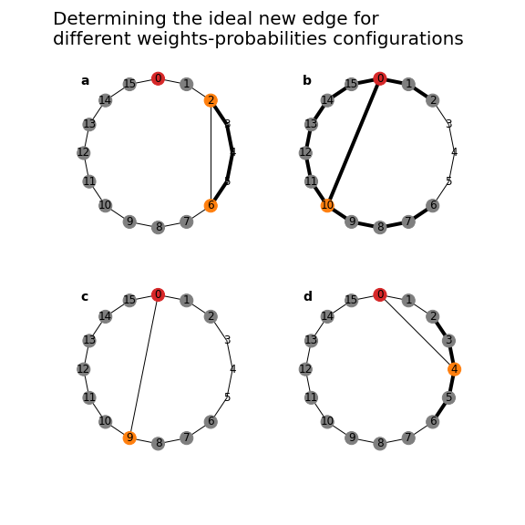
Figure 11: The figure shows how the configurations of the probabilities of the edges and the node’s weight affect the optimal new edge. Thick edges present edges with a high failure probability and large nodes radius represent large node weight. In each example, the edge’s low failure probability is $0.00001$, and the high failure probability is $0.01$. The low node weight is $1$, and the high weight is $1000$. In a,b, and c, we assign a low weight for the nodes in a segment. In a and d, we assign a high failure probability to the edges in the segment, but in b, we assign a high failure probability to the edges that are not in the segment. In a, by assigning high failure probabilities and low nodes weight for edges in a segment of the circle, the optimal new edge is on the boundary of the segment.

Appendix C Most reliable networks near zero

We aim to find the most reliable graph near zero for a fixed number of nodes and edges. First, we must define a reliable graph for small, large, or all $p$. The set $G_{n,m}$ includes all networks with $n$ nodes and $m$ edges.

Definition 1.

Most reliable graph

Given $n,m\in\mathbb{N}$ , define:

1. An uniformly most reliable graph is a graph $G\in G_{n.m}$ s.t $\forall p\in[0,1]:F_{G}(p)=\min_{H\in G_{n,m}}F_{H}(p)$

2. A most reliable graph near zero is a graph $G\in G_{n.m}$ s.t $\exists p^{\prime}\in[0,1]:\forall p\in[0,p^{\prime}]\,F_{G}(p)=\min_{H\in G_{n,m}}F_{H}(p)$

3. A most reliable graph near one is a graph $G\in G_{n.m}$ s.t $\exists p^{\prime}\in[0,1]:\forall p\in[p^{\prime},1]\,F_{G}(p)=\min_{H\in G_{n,m}}F_{H}(p)$

Identifying the uniformly most reliable graph is helpful because, in practice, we do not always have accurate information on the failure probability of network edges. This problem has been extensively researched by mathematicians[8]. The main difference is that their focus has been on the connectivity index called the all-terminal unreliability $Pr(G\text{ disconnected})$. While there are some known most reliable graphs relative to the all terminal unreliability, and some cases where it proved to have no such most reliable network[18], we prove in subsection C.2 that the only uniformly most reliable network relative to the SAIDI index is the star graph. This result encourages us to find the most reliable graph near zero(subsection C.3).

C.1 Methods

An alternative approach to represent the SAIDI polynomial with a more combinatorial interpretation exists. Instead of using the conventional polynomial expression $F_{G}=\sum_{k=0}^{m}a_{k}(G)p^{k}$, we can employ the binomial form

$$F_{G}=\sum_{k=1}^{m}b_{k}(G)p^{k}q^{m-k}$$ (44)

In this form, the value $b_{k}$ corresponds to the sum of the number of disconnected nodes resulting from each of the graph’s $k$ edges cut sets, which is deduced from the probability of having $k$ edge failures and $(m-k)$ operational edges, which is given by $p^{k}q^{m-k}$. The following equations can be used to convert between the two representations [12]:

$$a_{1} = b_{1};$$

$$a_{k} = \sum_{j=1}^{k}(-1)^{j+k}\binom{k}{j}b_{j}$$ (45)

$$b_{k} = a_{k}+\sum_{j=1}^{k-1}(-1)^{j+k-1}\binom{k}{j}b_{j}$$

The binomial SAIDI representation creates an effective method for finding the most reliable graphs.

Proposition 2.

Coefficients compression lemma[10]

Given two polynoms $f=\sum_{k=1}^{m}a_{k}p^{k}(1-p)^{m-k},g=\sum_{k=1}^{m}b_{k}p^{k}(1-p)^{m-k}$

1. If $\exists i$ s.t $\forall j\in[1,i):a_{j}=b_{j}$, and $a_{i}\leq b_{i}$, then there exist $p^{\prime}$ s.t $\forall p\in[0,p^{\prime}]:f(p)\leq g(p)$

2. If $\exists i$ s.t $\forall j\in[1,i):a_{m-j}=b_{m-j}$, and $a_{m-i}\leq b_{m-i}$, then there exist $p^{\prime}$ s.t $\forall p\in[p^{\prime},1]:f(p)\leq g(p)$

3. If $\forall i$ $a_{i}\leq b_{i}$, then $\forall p\in[0,1]:f(p)\leq g(p)$

We can follow a sequential approach to identify the most reliable graph for small or large values of $p$. We begin by identifying all the networks in $G_{n,m}$ that minimizes the first coefficient from each side. We then choose the network with the minimum value of the second coefficient from this subset, and so on. This process establishes a total order in $G_{n,m}$, the lexicographic order induced by the polynomial coefficient vector. Near zero, the lexicographic order is from the left to right of the coefficient vector; near one, the order is in the opposite direction. By sorting the polynomial coefficient vector from the $0$ to the $m$ coefficients, we can say that $G_{1}<G_{2}$ if and only if there exists a value $p^{\prime}$ such that for all $p$ in the range $[0,p^{\prime}],F_{G1}\leq F_{G2}$. Similarly, by sorting the coefficient vector from the $m$ to the $0$ coefficients, we can say that $G_{1}<G_{2}$ if and only if there exists a value $p^{\prime}$ such that for all $p$ in the range $[p^{\prime},1],F_{G1}\leq F_{G2}$.

We define a chain of network sets for a fixed $n,m\in\mathbb{N}$

$$A_{0} = \left\{G\in G_{n,m}\mid\forall H\in G_{n,m}:b_{0}(G)\leq b_{0}(H)\right\}$$

$$A_{k} = \left\{G\in A_{k-1}\mid\forall H\in A_{k-1}:b_{k}(G)\leq b_{k}(H)\right\}$$ (46)

$$B_{0} = \left\{G\in G_{n,m}\mid\forall H\in G_{n,m}:b_{m}(G)\leq b_{m}(H)\right\}$$

$$B_{k} = \left\{G\in B_{k-1}\mid\forall H\in B_{k-1}:b_{m-k}(G)\leq b_{m-k}(H)\right\}$$

Note that $A_{k}\subseteq A_{k-1}$ and that $B_{k}\subseteq B_{k-1}$. Also, the networks in $A_{k}$ or $B_{k}$ are smaller than the graph in $A_{k-1}$, $B_{k-1}$, respectively, relative to the appropriate order. The most reliable network near zero is in $A_{m}$, and the most reliable network near one is in $B_{m}$.

C.2 The only uniformly most reliable network is a star graph

Reliable networks near zero are from maximal connectivity. The connectivity of a network is the size of its smallest cut set. A network that is $k$-connected is in $A_{k-1}$ because all of its $(k-1)$ first coefficients are $0$. The network’s connectivity is at least its minimal degree because the set of all adjacent edges of a node is a cut set. From the hand-shaking lemma, a network with a minimal degree of $k$ has at least $kn/2$ edges. A super $k$-connected graph is a $k$-connected graph such that the only cut sets from size $k$ are the edges adjacent to a node. A super $k$-connected graph is in $A_{k}$ because it minimizes the $k$-coefficient. Finally, Bauer [19] found that a super $k$-connected $k$-regular graph for $k\geq 3$ always exists. We conclude that the most reliable network near zero has connectivity of at least $\lfloor\frac{2m}{n}\rfloor$. From the other side, we prove in the rest of the subsection that the most reliable networks near one have smaller connectivity which leads to the conclusion that there is no uniformly most reliable graph for non-tree graphs.

The most reliable networks near one are star multigraphs with almost equal edge multiplicity. Using the coefficient compression method, we must first minimize the coefficient $b_{m-1}$. This coefficient counted the number of connected nodes resulting from only one working edge. In that case, the only optionally connected nodes are the neighbors of the source, which imply that the optimal network is a star multigraph with the source in the middle.

The next step is to minimize $b_{m-2}$ over $B_{1}$. Mark the edge multiplicity of the edge $(s,t)$ for $t\in V(G)$ as $r_{t}$. $b_{m-2}$ represent two working edges. If the two edges are from the same nodes, $(n-1)$ nodes fail, and else, $(n-2)$ nodes fail.

$$b_{m-2}=\left([n-1]\sum_{i=1}^{m}\binom{r_{i}}{2}+[n-2]\left(\binom{m}{2}-\sum_{i=1}^{m}\binom{r_{i}}{2}\right)\right)$$ (47)

So in order to minimize $b_{m-2}$ we must minimize $\sum_{i=1}^{m}\binom{r_{i}}{2}=\frac{1}{2}(\sum_{i=1}^{m}r_{i}^{2}-m)$ i.e minimize $\sum_{i=1}^{m}r_{i}^{2}$. Proposition 3 states that this sum is minimized if the numbers $\{r_{i}\}$ differ by at most $1$. Finally, we conclude that the most reliable network near one is a star multigraph such that the edge multiplicity of any two edges differed at most by $1$.

It follows that the only uniformly most reliable network is a star graph in the case of $m=n-1$ or $n=2$. The minimal degree of the most reliable network near one is $\lfloor\frac{m}{n-1}\rfloor$. On the other hand, the connectivity of the most reliable network near zero is $\lfloor\frac{2m}{n}\rfloor$. Therefore, if $m\geq n$ and $n\neq 2$, the uniformly most reliable networks do not exist. Also, in the case of $m=n-1$, the graph is a tree with a SAIDI index of $\bar{F}_{G}=1-\mathbb{E}[q^{d}]$ for $d$ the number of nodes from each distance to the source. The multi-star graph minimizes this distance and is the uniformly most reliable network. Figure 12 shows an example of such a graph and compares it SAIDI with a super $3$-connected graph.

We conclude that reliable networks with unreliable components should minimize their distances from the source.

Proposition 3.

minimize the sum of powers with a constant sum.

Let $(x_{1}...,x_{k})\in\mathbb{N}^{k}$ s.t $\sum_{i=1}^{k}x_{i}=C$ for $s\geq 2$. The function $f_{s}=\sum_{i=1}^{k}x_{i}^{s}$ is minimized if and only if $\forall i,j:|x_{i}-x_{j}|\leq 1$

Proof.

If $k=2$ then $f_{s}=x_{1}^{s}+x_{2}^{s}$. $f_{s}$ has only one minimum point $x^{\prime}_{1}=x^{\prime}_{2}=\frac{x_{1}+x_{2}}{2}$. Therefore, the minimum in $\mathbb{N}$ is $x^{\prime}\in\{\lfloor\frac{x_{1}+x_{2}}{2}\rfloor,$$\lceil\frac{x_{1}+x_{2}}{2}\rceil\}$. For $k>2$, assume by contradiction and without loss of generality that there is a minimum point $X=(x_{1},...x_{k})\in\mathbb{N^{\text{k}}}$ of $f_{s}$ s.t $x_{1}=x_{2}+a$ for $|a|>2$ then for $Y=(\lfloor\frac{x_{1}+x_{2}}{2}\rfloor,\lceil\frac{x_{1}+x_{2}}{2}\rceil,x_{3},...,x_{k})$

$$f_{s}(Y) = \lfloor\frac{x_{1}+x_{2}}{2}\rfloor^{s}+\lceil\frac{x_{1}+x_{2}}{2}\rceil^{s}+\sum_{i=3}^{k}x_{i}^{k}$$

$$< \sum_{i=1}^{k}x_{i}^{k}=f_{s}(X)$$

From the other hand, all the points $X\in\mathbb{N}^{k}$s.t $\forall i,j:|x_{i}-x_{j}|\leq 1$, have the same value of $f_{s}(X)$ because, suppose that $\beta=\mod(C,k)$, then $x_{1}=\ldots=x_{\beta}=\lceil\frac{C}{k}\rceil$ and $x_{\beta-1}=\ldots=x_{k}=\lfloor\frac{C}{k}\rfloor$. ∎

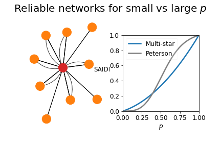
Figure 12: The figure compares reliable networks for small and large $p$. The multi-star graph is the most reliable for large p. The Peterson graph is super $3$-connected and hence reliable for small $p$.

C.3 Reliable network graphs are subdivisions of a cubic graphs

A sparse network is defined as one that maintains $m<1.5n$. For small values of $p$, the most reliable sparse network has a connectivity of two. Chains of edges with a degree of two can be contracted into a single chain, resulting in a structure graph where nodes are called hubs and edges are chains. The failure of each chain is $1-q^{c+1}$ for $c$ the number of nodes in the chain. By the ring-path formula(equation A.1), we can calculate the SAIDI index of the network using its structure graph. [11] shows that in the most reliable graph near zero relative to the all terminal polynomial, the structure graph is a $3$-connected and $3$-regular graph, and the chain’s lengths differ by at most one relative to the all terminal reliability. We prove that the result for the SAIDI polynomial is the same.

First, we minimize the second coefficient of $P_{2}f_{2}$ in equation A.1. The second coefficient is(equation 29) $\sum_{e^{\prime}\in S(G)}c(e^{\prime})^{3}+3c(e^{\prime})^{2}+2c(e^{\prime})$ where $c(e^{\prime})$ is the chain length. From proposition 3, because the sum of all chain’s lengths is constant, the minimum of the sum obtain if the chain lengths differ at most by $1$. In this scenario, the length of each chain is approximately $\frac{n-n^{\prime}}{m^{\prime}}$ where $n^{\prime}$ and $m^{\prime}$ are the number of nodes and edges in the structure graph, respectively.

The structure graph of the most reliable network near zero is a $3$-connected cubic graph with almost equal chains. To prove it, we first notice that in the structure graph, $m^{\prime}-n^{\prime}=m-n$ because by transforming a node with two edges to one edge, we preserve the difference $m-n$. To further minimize the second coefficient of $P_{2}f_{2}$, we need to minimize the chain’s length $\frac{n-n^{\prime}}{m^{\prime}}$. From the hand-shaking lemma and because the minimal degree of the structure graph is three, $3n^{\prime}\leq\sum_{v\in V(S(G))}deg(v)=2m^{\prime}$, which creates the upper bounds $m^{\prime}\leq 3(m-n)$ and $n^{\prime}\leq 2(m-n)$. The upper bound of the inequalities is received if the average degree in the structure graph is exactly $3$; hence, $S(G)$ is a cubic graph. If the structure graph is also a $3$-connected graph, the second coefficients of $P_{0}f_{0},P_{1}f_{1}$ and $F_{S(G)}$ are $0$. We conclude that all the networks in $A_{2}$ have a cubic $3$-connected structure graph with a chain length that differ by at most $1$.

We can minimize the network’s third coefficient by strategically placing the long chains. Assuming the structure graph is super 3-connected, we aim to reduce the number of long chains connected to the source node and minimize the number of long chains that share a connection with the same hub.

We can prove it using the risk formula 6. Let $e_{i}^{\prime}$ denote the length of the chain, given by $\alpha+r_{i}$, where $\alpha$ is a constant, and $r_{i}\in\{0,1\}$. In a super 3-connected graph, every three-order minimal cut set comprises one edge from each chain that connects to a particular hub. The risk associated with the cut sets originating from hub $v$ is given by:

$$\prod_{e_{i}^{\prime}\sim v}\left(\alpha+r_{i}+1\right)\left(D_{G}(E(v))+\frac{1}{2}\sum_{e^{\prime}\in X^{\prime}}(\alpha+r_{i})\right)$$ (48)

Here, $D_{G}(E(v))$ is 1 if $v$ is not the source, and $n-1$ otherwise. Consequently, we must avoid long chains that connect to the source. Furthermore, to minimize the factor $\prod_{e_{i}^{\prime}\sim v}(\alpha+r_{i}+1)$, we aim to reduce the number of long chains that connect to the same hub.

The $3$ connectivity of the structure graph is the most crucial structure graph factor in practice. Figure 13 compares different structure graphs with equal chains: a super $3$-connected graph, the worst $3$-connected graph with a given size, and a $k$-rings graph. All of those graphs have almost the same number of total nodes. Although the differences between the $k$-rings and the other graphs are significant, the difference between the optimal and worst $3$-connected graphs is minor, near zero. The figure also presents a family of super $3$-connected graphs, which are two connected rings. This simple form is used in subsection E.1 to create a reliable grid graph. The worst 3-connected graph is chosen by iterating all the cubic graphs with a given size using a database of all the cubic graphs with a given size [20][21]

Note that by adding $r+1$ redundant edges near zero, we approximate the SAIDI of the optimal graph as a ring with $(n-2r)/3r$ nodes

$$\bar{F}_{G}\overset{\text{order 2}}{=}\bar{F}_{ring}(\lfloor\frac{n-2r}{3r}\rfloor)\stackrel{{\scriptstyle n\gg 1}}{{\approx}}\frac{\left(1-2\frac{r}{n}\right)^{2}}{9r^{2}}\cdot\left[F_{ring}(n)\right]$$ (49)

On the other hand, a naive solution uses a $(r+1)$-rings approach, meaning setting a network with $(r+1)$ almost equal chains. The rings size in the $(r+1)$ rings solution is approximately $\frac{n}{r+1}$. We conclude that for a large value of $n$, the cubic structure graph approach is more than $9$ times better than the multi-rings approach.

Remark 1.

The optimal cubic structure graph solution is better than the naive $(r+1)$-rings solution by a factor of approximately

$$9\cdot\frac{r^{2}}{(r+1)^{2}(1-2\frac{r}{n})^{2}}$$ (50)

for a large value of $n$(figure 13).

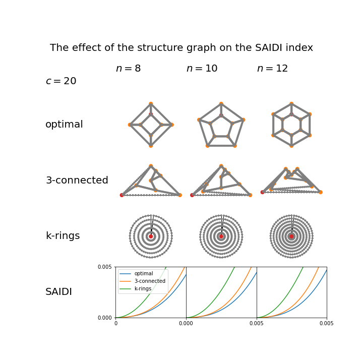
Figure 13: The figure tests the effect of the structure graph on the SAIDI index. The first row presents a family of super $3$-connected graphs, the second row presents the worst $3$-connected $3$-regular graph with a given size, and the third row presents the $k$-rings graph. Each column presents the number of nodes in the structure graph of the first two rows. Each chain of the first two rows contains $20$ nodes, and the number of nodes in each ring in the k-rings graph is chosen to have approximately the same amount of total nodes. The number of redundant edges in each column is the same. In the last row, we can compare the SAIDI index of the different topologies and conclude that the SAIDI difference between the $k$-rings and the other graphs are significant. However, the SAIDI difference between two graphs with a $3$-connected structure graph is minor.

C.4 Other reliability indexes

The construction rules of the most reliable graph near zero are maintained for other reliability indexes, such as the all-terminal reliability and pairwise reliability. The all-terminal reliability is the probability that the network is not connected $U_{G}=1-Pr(G\text{ connected})$. The pairwise reliability is the total number of disconnected node pairs $C_{G}=\sum_{v,u\in V(G)}Pr_{G}(v\nleftrightarrow u)$. The pairwise reliability is also the sum of the SAIDI index among all the optional sources in the graph. [11] proves that the most reliable sparse graph relative to the all terminal reliability index is a $3$-regular and $3$-connected structure graph with chain lengths that differ by at most one.

This equal-length chain property is also correct for the pairwise reliability index. If the structure graph is three-connected, the second coefficient of the polynom $Pr_{G}(v\nleftrightarrow u)$ for a pair of nodes $u$ and $v$ is the sum of all two-order cut sets that disconnect the two nodes. Those two-order cut sets are in the same chain. A pair of edges in the same chain with a distance $s$ disconnect $s(n-s)$ pairs of nodes if $n$ is the number of nodes in the graph. Each chain with $c+1$ edges has $c+1-s$ edges pairs with a distance $s$. it follows that the second coefficient of the pairwise polynomial is

$$b_{2}=\sum_{e_{i}^{\prime}\in E(S(G))}{\sum_{s=1}^{c_{i}}(c_{i}+1-s)\cdot s(n-s)}=\frac{1}{12}\sum_{e_{i}^{\prime}\in E(S(G))}c_{i}(c_{i}+1)(c_{i}+2)(2n-(c_{i}+1))$$ (51)

This sum is minimized if the chain’s length is differed by at most one. We can prove it by observe that the function $h(x)=x(x+1)(x+2)(2n-(x+1))$ is convex. We define two numbers $a<b$ and two numbers $\alpha=ta+(1-t)b$ and $\beta=(1-t)a+tb$. From the convex definition, $h(\alpha)+h(\beta)<h(a)+h(b)$. It follows that $h(\lfloor\frac{a+b}{2}\rfloor)+h(\lceil\frac{a+b}{2}\rceil)<h(a)+h(b)$, and similar to proposition 3, if the optimal solution has two chains length that differs by more than one, we can take the floor and the ceil of their average to get a better solution.

Appendix D Computation details

There are three significant algorithmic challenges in the network analysis. The first involves computing the SAIDI index. The second is identifying all minimal cut sets, and the third challenge is calculating the risk of a minimal cut set.

D.1 SAIDI computation

Calculating the SAIDI index of a graph is a computationally expensive task and is known to be an NP-hard problem [17]. The classical algorithm used to find the SAIDI index is the deletion-contraction algorithm, which has a time complexity of $O(2^{m})$, where $m$ is the number of edges in the graph. The deletion-contraction algorithm is a recursive algorithm where, in each step, one edge is chosen, and the probability space is split into the case where this edge is failing (deletion) and the case where the edge works (contraction). However, for certain families of graphs, a tree decomposition-based algorithm can be used to calculate the SAIDI index more efficiently.

Tree decomposition is a tree-like structure that enables a faster computation of certain graph properties. A tree decomposition of a graph $G$ is a pair $(T,X)$, where $T$ is a tree, and $X=\left\{X_{i}:i\in V(T)\right\}$ is a collection of sets, called bags, such that:

1. For each vertex $v\in G$, there exists at least one bag $X_{i}$ that contains $v$.

2. For each edge $(u,v)\in G$, there exists at least one bag $X_{i}$ that contains both $u$ and $v$.

3. For each vertex $v\in G$, the bags containing $v$ form a connected subtree of $T$.

The width of a tree decomposition is the maximum size of any bag minus one. The treewidth of a graph is the minimum width among all of its tree decompositions. There exists a linear-time algorithm that identifies if a graph’s treewidth is at most $\omega$, and if so, finds the tree decomposition with treewidth at most $\omega$ [22].

Tree decomposition algorithms can efficiently calculate the SAIDI index of graphs with small treewidth. Existing algorithms use tree decompositions to calculate the $K$-terminal reliability of a graph and the reaching probability between two nodes [23, 24]. The $K$-terminal reliability is the probability that a set $K$ of nodes is connected. These algorithms have a linear-time fixed-parameter complexity when the treewidth is used as the parameter. This means that the $K$-terminal reliability of graphs with treewidth smaller than a constant can be calculated in time that it linear in the number of nodes but exponential in the treewidth. Therefore, it is inefficient for graphs with large treewidth. By applying the algorithm for each node, a SAIDI index algorithm can be obtained with a complexity of $O(n^{2}\cdot\omega^{3}\cdot 2^{(\omega+2)(\omega+1)})$, where $n$ represents the number of nodes in the graph. Note that using the chain decomposition method and the ring-path formula in the tree decomposition-based approach, the algorithm’s complexity is linear in the number of hubs in the graph but exponential in the treewidth of the structure graph.

Although the exact SAIDI calculation is challenging, $k$-order approximations offer a polynomial time complexity in terms of the number of edges. In subsection A.5, we show that a 3rd-order approximation of the SAIDI index satisfies near zero. The complexity of the deletion-contraction $k$-order approximation is $O(m^{k})$. Similarly, the tree decomposition-based algorithm is polynomial in the treewidth of the graph. By combining the ring-path formula, the tree decomposition algorithm, and the observation that a third-order approximation is good in sparse graphs, we conclude that the SAIDI calculation of the graph is relatively fast.

D.2 Find minimal cut sets

Minimal cut sets of the structure graph are used to find structural risks. Finding those structural risks are important to understand the weak point of the network and decide which new edges are the most important. Because we focus on finding minimal cut sets of the structure graph and approximate the reliability index through 3rd-order cut sets, finding the relevant minimal cut sets of a sparse network is simpler.

Minimal cut sets are induced from connected subgraphs. Minimal cut sets separate the graph into exactly two connected components because otherwise, we can find a cut set contained in the minimal cut set. We can find the minimal cut sets by enumerating all the connected subgraphs and finding their boundary edges[25]. However, not every boundary edges of a connected subgraph is a minimal cut set. Therefore, after finding all the connected subgraphs of the structure graph, we need to check which cut sets are not minimal. We can also use the algorithm proposed in [26] or simply enumerate all the edges subsets of the graph with at most three edges and check which ones are minimal.

D.3 Calculating risks

After enumerating all the structure graph minimal cut sets, we can calculate the inter and structural risks of the network. The challenging part of calculating inter and structural risks is the probabilities $P_{2}(e^{\prime})$ and $Pr_{S(G)}(s\leftrightarrow X^{\prime})$ for a chain $e^{\prime}$ and structural minimal cut set $X^{\prime}$. The exact calculations can be done using the deletion-contraction or tree decomposition-based algorithm. However, suppose we calculate only a third-order approximation. In that case, those probabilities are much simpler: to calculate $P_{2}(e^{\prime})$, we only need to find bridges that disconnect the chain, and finding $Pr_{S(G)}(s\leftrightarrow X^{\prime})$ only requires to find cut sets with at most $(3-\left|X^{\prime}\right|)$ edges.

Appendix E Test cases

E.1 Grid

We use dynamic programming to calculate the optimal new edges in a grid, as shown in figure 5. The objective is to minimize the second coefficient of the super 3-connected network grid. The grid consists of m columns, and the source points are located in the top-left and bottom-right corners. Initially, the number of new edges between each adjacent column pair is defined, and the score of each new edge configuration is calculated by summing the ring second coefficient for each chain in the new graph. The goal is to minimize the score.

In the algorithm’s $i$ iteration, we calculate for each edge’s configuration between the $i$ and the ($i+1)$ columns the optimal edge’s configuration between columns $1$ to $i$. In the first step, we enumerate all the edge configurations between the first and the second columns. In the $i$ iteration, we already know the score of the optimal configurations on columns $1$ to $(i-1)$ given each edge configuration between the columns $(i-1)$ and $i$. We then enumerate each pair of edges configuration between the $(i-1$) to the $i$ columns and between the $i$ to the $(i+1)$ columns. The score of each configuration is the sum of the score on columns $1$ to $(i-1)$, which is already known, and the score of the $i$ columns.

The complexity of the algorithm is $O\left(m\cdot max_{i=1}^{m-1}\left(n_{i}^{k_{i}}\cdot n_{i+1}^{k_{i+1}}\right)\right)$ where $n_{i}$ is the length of the $i$ columns, and $k_{i}$ is the number of edges between the columns $i$, $(i+1)$. This example demonstrates the principle of modular design as implied by equation 15: the only effect of new edges within a subgraph on the rest of the graph is the partition probabilities of the subgraph boundaries. We can more efficiently determine the optimal new edges by computing the optimal inter-edges given the boundary configurations.

There are even better grid configurations. The grid topology, as presented above, has a major disadvantage because the east-west chains are from length $1$. To overcome this problem, we present, for example, a $5X100$ grid network with only four redundant edges, the same as the basic network topology(figure 14). However, the chains in the network are distributed more evenly, resulting in a more than $4$-fold improvement in the second coefficient of the SAIDI index. However, since the structure graph is not super $3$-connected, the improvement in SAIDI is only by a factor of $3.32$ for $p=0.0001$. We create the network by choosing a family of $3$-connected cubic graphs of two connected rings, as shown in figure 13, with six nodes to create five redundant edges and then fit the topology to the actual nodes. Using the cubic networks database[20], we can verify that there is no planner super $3$-connected cubic graph with six nodes. Because we have two sources, it is enough that each of them is from a degree of two. Therefore, we can split two of the chains into two chains, which results in a total of $11$ chains. Figure 14 presents the construction of this graph.

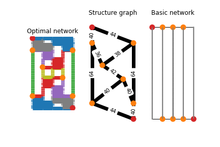
Figure 14: 5X100 grid configuration. The left network is a reliable network topology on a 5X100 grid. Each color represents a chain, and the red nodes are sources. The middle network is the structure graph of the network with the chain lengths. We can see that the chains are relatively equally distributed. The right network is the basic grid topology with the same amount of redundant edges.

E.2 Real networks analysis

We analyze data from the public electrical vehicle load capacity map by “Atlantic city electric” as presented in the main paper. The map goal as stated on the map website is to “represent areas on the distribution grid where it is reasonable capacity to accommodate electric vehicle charging infrastructure and other load sources with a lower probability of necessitating extensive equipment upgrades or line extensions that would add cost or time to projects”. The data was extracted manually in March 2023. A screen shot of the map is shown in figure 15.

To increase the network’s reliability, we identify short, optional road segments that can be used to create both chain-to-chain and inter-chain configurations, thereby improving the network’s reliability. We then experiment with various new edge configurations, aiming to minimize the second coefficient of the polynomial. For instance, two chains are relatively close in network 2. Therefore, we can use a chain-to-chain edge to connect them in the small gaps, which helps to enhance reliability. Finally, we enumerate the different combinations of these new edges and try to minimize the sum of the second coefficient of the SAIDI for a $3$-connected subgraph, represented as $\sum_{e\in S(G)}\frac{1}{6}(c(e)^{3}+3c(e)^{2}+2c(e))$. Similar to optimizing new edges in a grid, we can use a more sophisticated dynamic programming approach, whereby each new edge divides the chains into two segments, and we optimize each of these segments independently.

There are networks in which it is not worth investigating in new lines. For example, in network 3, apart from a crossing new edge between the two rings, there are no significant improvements we can make to the network’s reliability without resorting to expensive lines. Moreover, since the neighborhood is small, it is not worth investing in more lines. However, another optional improvement (version 2) is to move some nodes for the new crossing edge to reduce the length of the longer chain.

Name	Networks snapshots	Location(EPSG:4326)
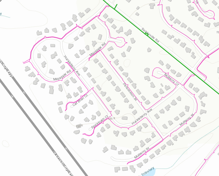
Network 1		(-75.0827636, 39.7401530)
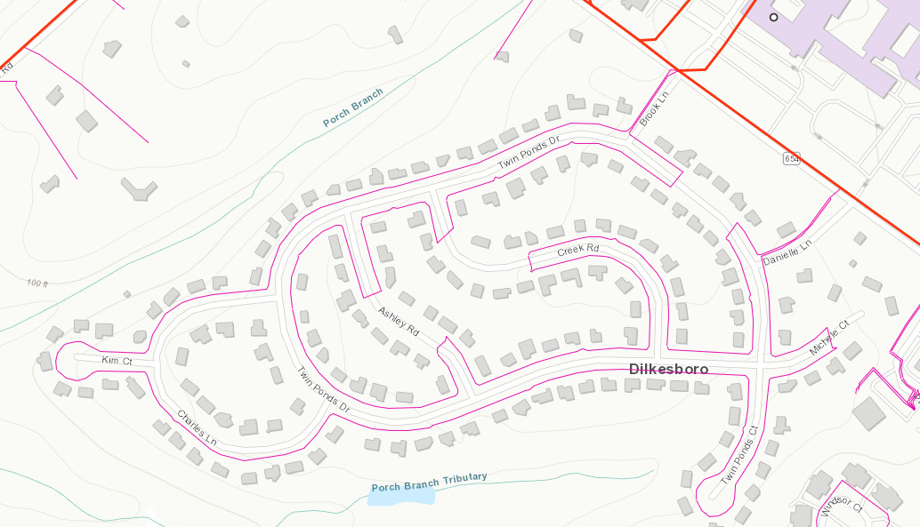
Network 2		(-75.0827636, 39.7401530)
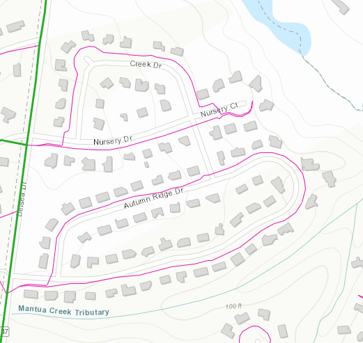
Network 3		(-75.112447,39.729465)

Figure 15: Snap shots of the networks from the “Atlantic city electric website”

References

- \bibcommenthead
- Prakash et al. [2016] Prakash, K., Lallu, A., Islam, F., Mamun, K.: Review of power system distribution network architecture, pp. 124–130 (2016). https://doi.org/10.1109/APWC-on-CSE.2016.030
- Islam et al. [2017] Islam, F.R., Prakash, K., Mamun, K.A., Lallu, A., Pota, H.R.: Aromatic network: A novel structure for power distribution system. IEEE Access 5, 25236–25257 (2017) https://doi.org/10.1109/ACCESS.2017.2767037
- Moore and Shannon [1956] Moore, E.F., Shannon, C.E.: Reliable circuits using less reliable relays. Journal of the Franklin Institute 262(3), 191–208 (1956)
- Canale et al. [2020] Canale, E., Rela, G., Robledo, F., Romero, P., Stábile, L.: Design of most-reliable cubic networks by augmentations. In: 2020 16th International Conference on the Design of Reliable Communication Networks DRCN 2020, pp. 1–6 (2020). https://doi.org/10.1109/DRCN48652.2020.1570611164
- [5] Mousa, S.K., Faraj, M.A., Amoura, F.K., Shuaieb, W.S.: Reliability indices evaluation of ring distribution systems without and with dg
- Anghel et al. [2007] Anghel, M., Werley, K.A., Motter, A.E.: Stochastic model for power grid dynamics. In: 2007 40th Annual Hawaii International Conference on System Sciences (HICSS’07), pp. 113–113 (2007). https://doi.org/10.1109/HICSS.2007.500
- Gertsbakh and Shpungin [2010] Gertsbakh, I., Shpungin, Y.: Models of network reliability. analysis, combinatorics and monte carlo (2010)
- Romero [2021] Romero, P.: Uniformly optimally reliable graphs: A survey. Networks (2021)
- ROMERO [2017] ROMERO, P.: Wagner and petersen are uniformly most-reliable graphs (2017)
- Bauer et al. [1987] Bauer, D., Boesch, F., Suffel, C., Van Slyke, R.: On the validity of a reduction of reliable network design to a graph extremal problem. IEEE Transactions on Circuits and Systems 34(12), 1579–1581 (1987) https://doi.org/%****␣tex.bbl␣Line␣175␣****10.1109/TCS.1987.1086075
- Wang and Zhang [1997] Wang, G., Zhang, L.: The structure of max -min m+ 1 graphs used in the design of reliable networks. Networks: An International Journal 30(4), 231–242 (1997)
- Rodionov and Rodionova [2016] Rodionov, A.S., Rodionova, O.: Practical notes on obtaining reliability polynomials. WSEAS Transactions on mathematics 15, 450–461 (2016)
- Harary [1962] Harary, F.: The maximum connectivity of a graph. Proceedings of the National Academy of Sciences of the United States of America 48(7), 1142 (1962)
- Baran and Wu [1989] Baran, M.E., Wu, F.F.: Network reconfiguration in distribution systems for loss reduction and load balancing. IEEE Transactions on Power Delivery 4(2), 1401–1407 (1989) https://doi.org/10.1109/61.25627
- Ali et al. [2020] Ali, M., Macana, C.A., Prakash, K., Islam, R., Colak, I., Pota, H.: Generating open-source datasets for power distribution network using openstreetmaps. In: 2020 9th International Conference on Renewable Energy Research and Application (ICRERA), pp. 301–308 (2020). https://doi.org/%****␣tex.bbl␣Line␣250␣****10.1109/ICRERA49962.2020.9242771
- Ross [1997] Ross, P.: Generalized hockey stick identities and n-dimensional blockwalking. The College Mathematics Journal 28(4), 325 (1997)
- Ball [1986] Ball, M.O.: Computational complexity of network reliability analysis: An overview. Ieee transactions on reliability 35(3), 230–239 (1986)
- Myrvold et al. [1991] Myrvold, W., Cheung, K.H., Page, L.B., Perry, J.E.: Uniformly-most reliable networks do not always exist. Networks 21(4), 417–419 (1991)
- Bauer et al. [1985] Bauer, D., Boesch, F., Suffel, C., Tindell, R.: Combinatorial optimization problems in the analysis and design of probabilistic networks. Networks 15(2), 257–271 (1985)
- Meringer [1999] Meringer, M.: Fast generation of regular graphs and construction of cages. Journal of Graph Theory 30(2), 137–146 (1999)
- Coolsaet et al. [2023] Coolsaet, K., D’hondt, S., Goedgebeur, J.: House of graphs 2.0: A database of interesting graphs and more. Discrete Applied Mathematics 325, 97–107 (2023)
- Bodlaender [1993] Bodlaender, H.L.: A linear time algorithm for finding tree-decompositions of small treewidth. In: Proceedings of the Twenty-fifth Annual ACM Symposium on Theory of Computing, pp. 226–234 (1993)
- Goharshady and Mohammadi [2020] Goharshady, A.K., Mohammadi, F.: An efficient algorithm for computing network reliability in small treewidth. Reliability Engineering & System Safety 193, 106665 (2020)
- Hagstrom [1983] Hagstrom, J.N.: Using the decomposition-tree of a network in reliability computation. IEEE Transactions on Reliability R-32(1), 71–78 (1983) https://doi.org/10.1109/TR.1983.5221478
- Alokshiya et al. [2019] Alokshiya, M., Salem, S., Abed, F.: A linear delay algorithm for enumerating all connected induced subgraphs. BMC bioinformatics 20, 1–11 (2019)
- Rebaiaia and Ait-Kadi [2013] Rebaiaia, M.-L., Ait-Kadi, D.: A new technique for generating minimal cut sets in nontrivial network. AASRI Procedia 5, 67–76 (2013)