Harnessing The Collective Wisdom:
Fusion Learning Using Decision Sequences From Diverse Sources

Abstract

Learning from the collective wisdom of crowds enhances the transparency of scientific findings by incorporating diverse perspectives into the decision-making process. Synthesizing such collective wisdom is related to the statistical notion of fusion learning from multiple data sources or studies. However, fusing inferences from diverse sources is challenging since cross-source heterogeneity and potential data-sharing complicate statistical inference. Moreover, studies may rely on disparate designs, employ widely different modeling techniques for inferences, and prevailing data privacy norms may forbid sharing even summary statistics across the studies for an overall analysis. In this paper, we propose an Integrative Ranking and Thresholding (IRT) framework for fusion learning in multiple testing. IRT operates under the setting where from each study a triplet is available: the vector of binary accept-reject decisions on the tested hypotheses, the study-specific False Discovery Rate (FDR) level and the hypotheses tested by the study. Under this setting, IRT constructs an aggregated, nonparametric, and discriminatory measure of evidence against each null hypotheses, which facilitates ranking the hypotheses in the order of their likelihood of being rejected. We show that IRT guarantees an overall FDR control under arbitrary dependence between the evidence measures as long as the studies control their respective FDR at the desired levels. Furthermore, IRT synthesizes inferences from diverse studies irrespective of the underlying multiple testing algorithms employed by them. While the proofs of our theoretical statements are elementary, IRT is extremely flexible, and a comprehensive numerical study demonstrates that it is a powerful framework for pooling inferences.

Keywords: Crowdsourcing, E-values, False Discovery Rate, Fusion learning, Integrative inference, Meta-analysis

1 Introduction

Learning from the wisdom of crowds is the process of synthesizing the collective wisdom of disparate participants for performing related tasks, and has evolved into an indispensable tool for modern scientific inquiry. This process is also known as ‘Crowdsourcing’, which has generated tremendous societal benefits through novel drug discovery (Chodera et al., 2020), new machine learning algorithms (Sun et al., 2022), product design (Jiao et al., 2021) and crime control (Logan, 2020), to name a few. Harnessing such collective wisdom allows incorporating diverse opinions as well as expertise into the decision-making process and ultimately broadens the transparency of scientific findings (Surowiecki, 2005).

Synthesizing the collective wisdom of crowds is related to the statistical notion of fusion learning from multiple data sources or studies (Liu et al., 2022; Guo et al., 2023). Over the past decade, techniques for such fusion learning have found widespread use for incorporating heterogeneity into the underlying analysis and increasing the power of statistical inference. For instance, in recent years the accrescent volume of gene expression data available in public data repositories, such as the Gene Expression Omnibus (GEO) (Barrett et al., 2012) and Array Express (Rustici et al., 2012), have facilitated the synthesis and reuse of such data for meta-analysis across multiple studies. Biologists can use OMiCC (Shah et al., 2016), a crowdsourcing web platform, for generating and testing hypotheses by integrating data from diverse studies. Relatedly, sPLINK (Nasirigerdeh et al., 2022), a hybrid federated tool, allows conducting privacy-aware genome-wide association studies (GWAS) on distributed datasets. In distributed multisensor systems, such as wireless sensor networks, each node in the network evaluates its designated region in space by conducting simultaneous test of several hypotheses. The decision sequence is then transmitted to a fusion center for processing. Sensor fusion techniques are used to synthesize the data from multiple sensors, which provides improved accuracy and statistically powerful inference than that achieved by the use of a single sensor alone. (Hall and Llinas, 1997; Shen and Wang, 2001; Jamoos and Abuawwad, 2020)

However, fusing inferences from diverse sources is challenging for several reasons. First, cross-source heterogeneity and potential data-sharing complicate statistical inference. For instance, in microarray meta-analysis, an integrative false discovery rate (FDR) analysis of the multiple hypotheses often require making additional assumptions such as study independence and strong modeling assumptions to capture between-study heterogeneity. Second, prevailing data privacy norms may forbid sharing even summary statistics across the studies for an overall analysis. This is particularly relevant in the context of genomic data where NIH (National Institutes of Health) restricts the availability of dbGaP (database of Genotypes and Phenotypes) data to approved users (Couzin, 2008; Zerhouni and Nabel, 2008). Also, in wireless sensor networks, communication limits may restrict sharing all information from the nodes to the fusion center. Third, in the case of meta-analysis where fusion learning is widespread, different studies may rely on disparate designs and widely different modeling techniques for individual inferences. Besides introducing algorithmic randomness into the individual inferences, it is also unclear how such inferences can be integrated and subsequently interpreted. Fourth, often significant statistical and computational experience is required for integrating the individual inferences. This may preclude investigators without substantial statistical training to perform such analyses.

In this paper, we develop a framework for fusion learning in multiple testing that seeks to overcome the aforementioned challenges of integrative inference across multiple data sources. Our framework, which we call IRT for Integrative Ranking and Thresholding, operates under the setting where from each study a triplet is available: the study-specific vector of binary accept / reject decisions on the tested hypotheses, the FDR level of the study and the hypotheses tested by the study. Under this setting, the IRT framework consists of two key steps: in step (1) IRT utilizes the binary decisions from each study to construct nonparametric evidence indices which serve as measures of evidence against the corresponding null hypotheses, and in step (2) the evidence indices across the studies are fused into a discriminatory measure that ranks the hypotheses in the order of their likelihood of being rejected. The proposed fusion learning framework has several distinct advantages. First, the IRT framework guarantees an overall FDR control under arbitrary dependence between the evidence indices as long as the individual studies control the FDR at their desired levels. Second, IRT is extremely simple to implement and is broadly applicable without any model assumptions. This particular aspect is especially appealing because IRT synthesizes inferences from diverse studies irrespective of the underlying multiple testing algorithms employed by the studies. Third, the evidence indices in our framework are closely related to “$e-$values” (see Shafer (2021); Vovk and Wang (2021); Grünwald et al. (2023); Ramdas et al. (2020); Wasserman et al. (2020) for an incomplete list) for hypothesis testing. Besides being a natural counterpart to the popular $p-$values in statistical inference, $e-$values are relatively more robust to model misspecification and particularly to dependence between the $p-$values. In our numerical experiments, we find that when the $p-$values are exchangeable IRT is substantially more powerful than methods that rely on a conversion from $p-$values to $e-$values for pooling inferences. For almost a century, $e-$values have been used in Statistics, often disguised as likelihood ratios, Bayes factors, stopped nonnegative supermartingales. See Ramdas et al. (2022) for a survey on additional settings, such as betting scores, game-theoretic statistics and safe anytime-valid inference, where $e-$values arise naturally. Finally, to the best of our knowledge, IRT is the first fusion learning framework for multiple testing that relies on the binary decision sequences which are relatively more private than summary statistics. We rely on a novel construction of $e-$values from the accept-reject decisions which are also related to the all-or-nothing bet of Shafer (2021) for testing a single null hypothesis.

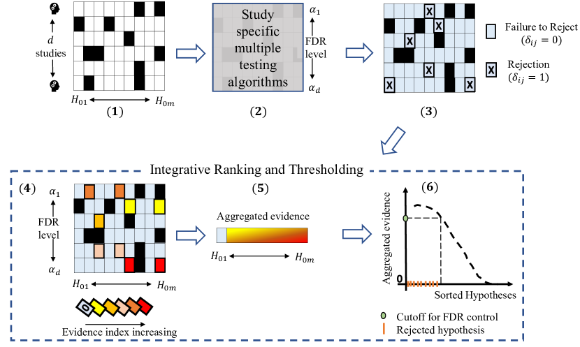
Figure 1: A pictorial representation of the IRT framework. In panel (1) $d$ studies are testing a study-specific subset of $m$ null hypotheses. Here the black solid squares represent hypotheses that are not tested by the individual studies. In panel (2), these studies use different multiple testing algorithms that are designed to control their respective FDR at level $\alpha_{j},~{}j=1,\ldots,d$. The ‘X’-marked squares in panel (3) depict the rejected hypotheses and represent the data that is available to the IRT framework. It includes the binary decision vectors $\delta_{ij}$ from each study, the study-sepcific FDR level $\alpha_{j}$ and the subset of $m$ hypotheses evaluated by each study. In panel (4), the IRT framework converts each binary decision into a nonparametric evidence index such that a higher index, displayed in a darker shade of red, represents a larger likelihood for rejecting that study-specific null hypothesis. In panel (5), the study-specific evidence indices are fused in a manner such that the aggregated indices rank the $m$ hypotheses and, as demonstrated in panel (6), the rankings can be used to determine a cutoff for valid FDR control at a pre-determined level $\alpha$.

1.1 Outline of the proposed approach

Figure 1 provides a pictorial representation of our setup and an overview of the IRT framework. A precise formulation and formal mathematical statements are deferred until Section 2. Panel (1) of Figure 1 represents a scenario where $d$ studies are testing a study-specific subset of $m$ null hypotheses. Here the black solid squares represent hypotheses that are not tested by the individual studies. In Panel (2), these individual studies use different multiple testing algorithms that are designed to control their respective FDR at level $\alpha_{j},~{}j=1,\ldots,d$. The ‘X’-marked squares in Panel (3) depict the rejected hypotheses and represent the data that is available to the IRT framework for synthesis. It includes the binary decisions $\delta_{ij}$ from each study, the study-sepcific FDR level $\alpha_{j}$ and the subset of $m$ hypotheses evaluated by each study. Panels (4)-(6) illustrate the IRT framework. Particularly, in Panel (4), the IRT framework converts each binary decision $\delta_{ij}$ into a nonparametric evidence index such that a higher index, displayed in a darker shade of red, represents a stronger conviction against that study-specific null hypothesis. In Panel (5), the study-specific evidence indices are fused in a manner such that the aggregated indices rank the $m$ hypotheses and, as demonstrated in Panel (6), the rankings can be used to determine a cutoff for valid FDR control at a pre-determined level $\alpha$.

1.2 Related literature

The IRT framework is related to multiple strands of literature, which includes FDR control using $e-$values, integrative multiple testing under data-privacy and algorithmic derandomization. Next, we discuss how IRT differs from these existing body of works.

Recently, there has been a proliferation of interest in developing methods for simultaneous hypotheses testing using $e-$values. See, for instance, Wang and Ramdas (2022); Ignatiadis et al. (2022); Chi et al. (2022); Vovk and Wang (2023); Xu and Ramdas (2023) and the references therein. In these works, the $e-$values are typically constructed from either $p-$values or likelihood ratios. In contrast, the generalized $e-$values (Wang and Ramdas, 2022; Ren and Barber, 2022) in our setting arise from the accept / reject decisions of the corresponding null hypotheses and are constructed in a nonparametric fashion.

The literature on the evolving field of integrative multiple testing under data-privacy is also related to our work. For instance, under the restricted data-sharing mechanism of Wolfson et al. (2010), Liu et al. (2021), henceforth Liu21, propose an integrative high-dimensional multiple testing framework with asymptotic FDR control. Our work differs from Liu21 on two main aspects. First, for our setting we consider a relatively more stringent data-privacy regime where the studies are only allowed to share their decision sequences, the FDR level and the hypotheses tested by them. Second, the integrative FDR control offered by IRT is non-asymptotic if the individual studies guarantee a non-asymptotic control of their respective FDR levels (see Section 4.3). This aspect is particularly appealing when the underlying multiple testing problem is small-scale.

Numerous methods have been proposed for mitigating algorithmic randomness in recent years. For instance, Bashari et al. (2023) propose a method to aggregate conformal tests for outliers obtained with repeated splits of the same data set, while controlling the FDR. In the context of high dimensional variable selection, Ren and Barber (2022) develop a methodology for derandomizing model-X knockoffs (Barber and Candès, 2015; Candes et al., 2018) with provable FDR control while Dai et al. (2022, 2023) develop a multiple data-splitting method with asymptotic FDR control to stabilize variable selection results. The IRT framework can be similarly viewed as a method for mitigating algorithmic randomness that may potentially arise from the use of myriad multiples testing procedures for FDR control by the $d$ studies. Crucially, however, our framework does not rely on hard-to-verify assumptions for FDR control, such as Dai et al. (2022, 2023), and in contrast to Ren and Barber (2022); Bashari et al. (2023), IRT only requires access to the binary decision vector of each study for integrative FDR control.

1.3 Organization

The article is laid out as follows: Section 2 presents our formal problem statement. The IRT framework is introduced in Section 3 and its operational characteristics are discussed in Section 4. A real data illustration is presented in Section 5 while Section 6 reports the empirical performance of IRT on synthetic data. The article concludes with a summary in Section 7.

2 Problem statement

Throughout the paper, we write $\mathcal{M}=\{1,\dots,m\}$ and consider testing $m$ null hypotheses $H_{01},\dots,H_{0m}$. Denote $\mathcal{H}_{0}=\{i:H_{0i}\ \text{is true}\}$ and $\mathcal{H}_{1}=\mathcal{M}/\mathcal{H}_{0}$, respectively, as the set of true null and non-null hypotheses. Let $\mathbb{I}(\cdot)$ denote the indicator function that returns 1 if condition is true and 0 otherwise, and denote $\|\bm{a}\|_{p}$ as the $l_{p}$-norm of the vector $\bm{a}$. In the sequel, $a\vee b$ will denote $\max(a,b)$ for two real numbers $a$ and $b$.

We consider a setting where the $\mathcal{M}$ hypotheses are tested by $d$ studies with study $j$ testing $\mathcal{M}_{j}\subseteq\mathcal{M}$ hypotheses. Here $\cup_{j=1}^{d}\mathcal{M}_{j}=\mathcal{M}$ and $|\mathcal{M}_{j}|=m_{j}$ so that $\sum_{j=1}^{d}m_{j}\geq m$. Let $\theta_{i}=\mathbb{I}(H_{0i}\text{~{}is false})$ be an indicator function that gives the true state of the $i$th testing problem and denote $\delta_{ij}\in\{0,1\}$ as the decision that study $j$ makes about hypothesis test $i\in\mathcal{M}_{j}$, with $\delta_{ij}=1$ being a decision to reject $H_{0i}$. Denote the vector of all $m_{j}$ decisions $\bm{\delta}_{j}=(\delta_{1j},\cdots,\delta_{m_{j}j})\in\{0,1\}^{m_{j}}$. A selection error, or false positive, occurs if study $j$ asserts that $H_{0i},~{}i\in\mathcal{M}_{j}$, is false when it actually is not. In multiple testing problems, such false positive decisions are inevitable if we wish to discover interesting effects with a reasonable power. Instead of aiming to avoid any false positives, a practical goal is to keep the false discovery rate (FDR) (Benjamini and Hochberg, 1995) small, which is the expected proportion of false positives among all selections,

$$\text{FDR}(\bm{\delta}_{j})=\mathbb{E}\left[\text{FDP}(\bm{\delta}_{j})\right]~{}\text{where FDP}(\bm{\delta}_{j})=\dfrac{\sum_{i\in\mathcal{M}_{j}}(1-\theta_{i})\delta_{ij}}{\sum_{i\in\mathcal{M}_{j}}\delta_{ij}\vee 1}.$$

The power of a testing procedure is measured by the expected number of true positives (ETP) where,

$$\mbox{ETP}(\bm{\delta}_{j})=\mathbb{E}\Big{(}\sum_{i\in\mathcal{M}_{j}}\theta_{i}\delta_{ij}\Big{)}=\mathbb{E}\Big{(}\sum_{i\in\mathcal{M}_{j}}\mathbb{I}(H_{0i}\text{ is false})\delta_{ij}\Big{)}.$$

Hence, the multiple testing problem for study $j$ can be formulated as

$$\text{maximize}_{\bm{\delta}_{j}}~{}\text{ETP}(\bm{\delta}_{j})~{}\text{subject to }\mbox{FDR}(\bm{\delta}_{j})\leq\alpha_{j},$$

where $\alpha_{j}\in(0,1)$ is a pre-specified cap on the maximum acceptable FDR for the $j^{th}$ study.

Our goal is to conduct inference for $\bm{\theta}=(\theta_{1},\ldots,\theta_{m})$ by fusing the evidence available in the binary decision sequences $\bm{\delta}_{j}$ provided by the $d$ studies. To do that we develop an integrative ranking and thresholding procedure that operates on the triplet $\mathcal{D}_{j}=\{\bm{\delta}_{j},\alpha_{j},\mathcal{M}_{j}\}$ available from each study and provably controls the FDR within a pre-determined level $\alpha\in(0,1)$.

3 Integrative ranking and thresholding using binary decision sequences

In this section we present IRT, an Integrative Ranking and Thresholding framework that involves three steps. In Step 1, IRT utilizes the binary decision sequence $\bm{\delta}_{j}$ from study $j$ to construct a measure of evidence against the null hypotheses $\mathcal{M}_{j}$. In Step 2, this evidence is aggregated into a discriminatory measure such that for each null hypothesis $H_{0i}$, a large aggregated evidence implies a higher likelihood of rejecting $H_{0i}$. In the final Step 3, the rankings provided by the aggregated evidence are used to determine a cutoff for FDR control. In what follows, we describe each of these steps in detail while Algorithm 1 summarizes the discussion below.

Step 1: Evidence construction

IRT uses the information in $\mathcal{D}_{j}$ to construct an evidence index $e_{ij}$ as follows:

$$e_{ij}=w_{j}\dfrac{\delta_{ij}}{\|\bm{\delta}_{j}\|_{0}\vee 1},~{}i\in\mathcal{M}_{j},$$ (1)

where the evidence weights $w_{j}=m_{j}/\alpha_{j}$. The evidence weights in Equation (1) capture the relative importance of a rejection across the $d$ studies and, hence, play a key role in differentiating among them. For study $j$, the evidence weight is distributed evenly across the rejected hypotheses. Moreover, this weight is higher if study $j$ has tested more hypotheses (larger $m_{j}$) and more conservative (smaller $\alpha_{j}$). This is in perfect accordance with our intuition since the evidence needed to reject a hypothesis increases if the number of hypotheses tested increases or the target FDR level decreases. For example, if only one hypothesis is tested then rejecting that null hypothesis when the $p-$value is below $\alpha$ guarantees FDR is controlled at level $\alpha$. However, if more than one hypothesis is tested then rejecting null hypotheses with $p-$value atmost $\alpha$ does not guarantee FDR control at level $\alpha$.

The evidence indices $\bm{e}_{j}=\{e_{ij}:i\in\mathcal{M}_{j}\}$ in Equation (1) are related to $e-$values for hypothesis testing, which serve as a natural counterpart to the widely adopted $p$-values. A non-negative random variable $e$ is an “$e-$value” if $\mathbb{E}[e]\leq 1$ under the null hypothesis. A large $e-$value provides evidence against the null hypothesis. See Vovk and Wang (2021) for a background on $e-$values for hypothesis testing. Recently, Wang and Ramdas (2022); Ren and Barber (2022) introduce the concept of generalized $e-$values which are defined as follows:

Definition 1 (generalized $e-$values).

Let $\bm{e}=\{e_{1},e_{2},\dots,e_{m}\}$ be a collection of random variables associated with the null hypotheses $H_{01},H_{02},\dots,H_{0m}$. Then $\bm{e}$ is a set of generalized $e-$values if $\sum_{i\in\mathcal{H}_{0}}\mathbb{E}(e_{i})\leq m$.

Theorem 1 establishes that the evidence indices in Equation (1) are generalized $e-$values.

Theorem 1.

Suppose the $j^{th}$ study controls FDR at level $\alpha_{j}$. Then $\bm{e}_{j}$ are generalized $e-$values associated with $\mathcal{H}_{0j}=\{H_{0i}:i\in\mathcal{M}_{j}\}$.

Proof.

We have

$$\sum_{i\in\mathcal{H}_{0j}}\mathbb{E}(e_{ij}) =\dfrac{m_{j}}{\alpha_{j}}\mathbb{E}\Big{(}\dfrac{\sum_{i\in\mathcal{H}_{0j}}\delta_{ij}}{\|\bm{\delta}_{j}\|_{0}\vee 1}\Big{)}$$

$$=\dfrac{m_{j}}{\alpha_{j}}\text{FDR}(\bm{\delta}_{j})\leq m_{j},$$

where the last inequality follows from the fact that study $j$ controls FDR at level $\alpha_{j}$. ∎

Next, we discuss Step 1 under the light of an important special case of testing a single hypothesis. Suppose $m=d=1$ and we are testing $H_{01}$. Then, in this setting the most powerful testing procedure is the one that rejects $H_{01}$ when the underlying $p-$value, say $p$, is at most $\alpha_{1}$, i.e $\delta_{11}=\mathbb{I}\{p\leq\alpha_{1}\}$. The corresponding evidence index,

$$e_{11} = (1/\alpha_{1})\mathbb{I}\{\delta_{11}=1\},$$ (2)

is the most powerful $e-$value that is equivalent to this testing procedure at threshold $1/\alpha_{1}$. The evidence index in Equation (2) is also known as the all-or-nothing bet (Shafer, 2021) against $H_{01}$ and provides another intuitive interpretation of the evidence indices in Equation (1) as follows: if the $j^{th}$ study controls FDR at level $\alpha_{j}$ then $\bm{e}_{j}$ are scaled all-or-nothing bets against the null hypotheses in $\mathcal{M}_{j}$ where the scaling $m_{j}/(\|\bm{\delta}_{j}\|_{0}\vee 1)$ ensures that if all the null hypotheses corresponding to the non-zero bets ($e_{ij}\neq 0$) in $\mathcal{M}_{j}$ are true then the probability that the sum of those non-zero bets exceed $m_{j}/\alpha_{j}$ is at most $\alpha_{j}$.

Step 2: Evidence aggregation

Denote $n_{i}=\sum_{j=1}^{d}\mathbb{I}\{i\in\mathcal{M}_{j}\}$ as the number of times hypothesis $H_{0i}$ is tested by the $d$ studies and let $n=\max\{n_{1},\ldots,n_{m}\}\geq 1$. IRT aggregates the evidence indices $\bm{e}_{j}$ across the studies as follows:

$${e}_{i}^{\sf agg}=\dfrac{1}{n}\sum_{j=1}^{d}e_{ij}\mathbb{I}\{i\in\mathcal{M}_{j}\}.$$ (3)

In Equation (3), $e_{i}^{\sf agg}$ represents the aggregated evidence across all studies that test hypothesis $H_{0i}$. When each study tests all the $m$ hypotheses, i.e $n_{i}=n=d$, then $e_{i}^{\sf agg}$ is the arithmetic mean of the $d$ evidence indices corresponding to hypothesis $i$, which dominates any symmetric aggregation function by Proposition 3.1 of Vovk and Wang (2021). However, when $n_{i}$ are different, the aggregation scheme in Equation (3) is a natural counterpart to the arithmetic mean of the $d$ evidence indices. Furthermore, in this setting Theorem 2 establishes that $\bm{e}^{\sf agg}=\{e_{1}^{\sf agg},\ldots,e_{m}^{\sf agg}\}$ are generalized $e-$values associated with $\mathcal{H}_{0}$.

Theorem 2.

Suppose study $j$’s testing procedure controls FDR at level $\alpha_{j}$. Then $\bm{e}^{\sf agg}$ are generalized $e-$values associated with $\mathcal{H}_{0}$.

Proof.

We have,

$$\sum_{i\in\mathcal{H}_{0}}\mathbb{E}(e_{i}^{\sf agg}) =\dfrac{1}{n}\sum_{i\in\mathcal{H}_{0}}\sum_{j=1}^{d}\dfrac{m_{j}}{\alpha_{j}}\mathbb{E}\Big{(}\dfrac{\delta_{ij}}{\|\bm{\delta}_{j}\|_{0}\vee 1}\Big{)}\mathbb{I}\{i\in\mathcal{M}_{j}\}$$

$$=\dfrac{1}{n}\sum_{j=1}^{d}\dfrac{m_{j}}{\alpha_{j}}\mathbb{E}\Big{(}\dfrac{\sum_{i\in\mathcal{H}_{0j}}\delta_{ij}}{\|\bm{\delta}_{j}\|_{0}\vee 1}\Big{)}$$

$$\leq\dfrac{1}{n}\sum_{j=1}^{d}m_{j}.$$ (4)

But $\sum_{j=1}^{d}m_{j}=\sum_{j=1}^{d}\sum_{i=1}^{m}\mathbb{I}(i\in\mathcal{M}_{j})=\sum_{i=1}^{m}n_{i}$. Substituting this in Equation (3) and noting that $\sum_{i=1}^{m}n_{i}\leq mn$ establishes that $\sum_{i\in\mathcal{H}_{0}}\mathbb{E}(e_{i}^{\sf agg})\leq m$, which completes the proof. ∎

In Section 4.1 we discuss an alternative evidence aggregation scheme where $n$ is replaced by $n_{i}$ in Equation (3) and $e_{i}^{\sf agg}$ continue to be generalized $e-$values under some additional assumptions on the data generating process for each study.

Step 3: FDR control at level $\alpha$

In the context of multiple testing with $e-$values, Wang and Ramdas (2022) proposed the $e-$BH procedure that controls the FDR at level $\alpha$ even under unknown arbitrary dependence between the $e-$values. The $e-$BH procedure is related to the well-known Benjamini-Hochberg (BH) procedure (Benjamini and Hochberg, 1995) and can be summarized as follows: let $e_{i}$ be a generalized $e-$value associated with the null hypothesis $H_{0i},~{}i=1,\ldots,m$. Denote $e_{(1)}\geq\ldots\geq e_{(m)}$ as the ordered $e-$values from largest to smallest. The rejection set under the $e-$BH procedure is given by $\{i:e_{(i)}\geq m/(\alpha k_{\alpha})\}$ where

$$k_{\alpha}=\max\Big{(}i\in\mathcal{M}:e_{(i)}\geq\dfrac{m}{i\alpha}\Big{)}.$$

In step 3, IRT uses $\bm{e}^{\sf agg}$ as input for the $e-$BH procedure to get the final rejection set and, in conjunction with Theorem 2, the IRT framework controls FDR at level $\alpha$.

We summarize the aforementioned three steps in Algorithm 1. Readers interested in the numerical performance of IRT may skip to sections 5 and 6 without any significant loss of continuity.

Algorithm 1 Integrative Ranking and Thresholding (IRT)

Inputs: $\mathcal{D}_{j}=\{\bm{\delta}_{j},\alpha_{j},\mathcal{M}_{j}\}$ for $j=1,\ldots,d$ studies.

1:Step 1: Evidence construction

2:for $j=1,\dots,d$ do

3:     Construct $e_{ij}={m_{j}\delta_{ij}}\big{/}\{\alpha_{j}(\|\bm{\delta}_{j}\|_{0}\vee 1)\}$ for each $i\in\mathcal{M}_{j}$.

4:end for

5:Step 2: Evidence aggregation

6:for $i=1,\dots,m$ do

7:     if The conditions of Theorem 3 are satisfied, then

8:         Calculate ${e}_{i}^{\sf agg}=\sum_{j=1}^{d}\frac{1}{n_{i}}e_{ij}\mathbb{I}\{i\in\mathcal{M}_{j}\}.$

9:     else

10:         Calculate $e_{i}^{\sf agg}=\frac{1}{n}\sum_{j=1}^{d}e_{ij}\mathbb{I}\{i\in\mathcal{M}_{j}\}$.

11:     end if

12:end for

13:Step 3: FDR control

14:($e-$BH procedure) Given a designated FDR level $\alpha\in(0,1)$, choose the threshold $k_{\alpha}$ as:

$$k_{\alpha}=\max\Big{(}i\in\mathcal{M}:e^{\sf agg}_{(i)}\geq\dfrac{m}{i\alpha}\Big{)}.$$ (5)

Output: Reject all $H_{0i}$ with $e^{\sf agg}_{i}\geq m/(\alpha k_{\alpha})$.

4 Discussion

In this section, we make several remarks related to the operational characteristics of the IRT framework.

4.1 Alternative evidence aggregation scheme

Suppose $\theta_{i}$ are random variables with an exchangeable joint distribution and conditional on $\theta_{i}$, the summary statistics $X_{ij}$ for study $j$ are generated according to the following model:

$$X_{ij}~{}\mid~{}\theta_{i}\stackrel{{\scriptstyle ind.}}{{\sim}}(1-\theta_{i})f_{0j}+\theta_{i}f_{1j},$$ (6)

where $f_{0j},f_{1j}$ represent, respectively, the null and non-null densities of $X_{ij}$. Under this setup a new aggregation scheme, analogous to Equation (3), can be defined as follows:

$${e}_{i}^{\sf agg*}=\sum_{j=1}^{d}\dfrac{1}{n_{i}}e_{ij}\mathbb{I}\{i\in\mathcal{M}_{j}\}.$$ (7)

Theorem 3 establishes that $\bm{e}^{\sf agg*}=\{e_{1}^{\sf agg*},\ldots,e_{m}^{\sf agg*}\}$ continue to be generalized $e-$values.

Theorem 3.

Suppose $\theta_{i}$ are random and their joint distribution exchangeable. Assume study $j$’s testing procedure controls FDR at level $\alpha_{j}$. Then $\bm{e}^{\sf agg*}$ in Equation (7) are generalized $e-$values associated with $\mathcal{H}_{0}$.

Proof.

We have

$$\sum_{i=1}^{m_{j}}\mathbb{E}\{e_{ij}\mathbb{I}(\theta_{i}=0)\}=\sum_{i=1}^{m_{j}}\mathbb{E}\{e_{ij}|\theta_{i}=0\}\mathbb{P}(\theta_{i}=0).$$

By exchangeability, $\mathbb{P}(\theta_{i}=0)$ is independent of $i$, and by Equation (6) $\mathbb{E}\{e_{ij}|\theta_{i}=0\}$ is also independent of $i$. Since $\sum_{i=1}^{m_{j}}\mathbb{E}\{e_{ij}\mathbb{I}(\theta_{i}=0)\}\leq m_{j}$ it follows that $\mathbb{E}\{e_{ij}\mathbb{I}(\theta_{i}=0)\}\leq 1$. Hence,

$$\sum_{i=1}^{m}\mathbb{E}\{e_{i}^{\sf agg*}\mathbb{I}(\theta_{i}=0)\} =\sum_{i=1}^{m}\sum_{j=1}^{d}\frac{1}{n_{i}}\mathbb{E}\{e_{ij}\mathbb{I}(i\in\mathcal{M}_{j})\mathbb{I}(\theta_{i}=0)\}$$

$$\leq\sum_{i=1}^{m}1=m.$$

∎

The advantage of $\bm{e}^{\sf agg*}$ over $\bm{e}^{\sf agg}$ is that the former provide a relatively better ranking of the hypotheses, which can lead to an improved power at the same FDR level $\alpha$. Our numerical experiments in Section 6 demonstrate that this is indeed true when the data generating mechanism obeys Equation (6) and the conditions of Theorem 3.

4.2 The choice of $\alpha$

The IRT procedure guarantees an overall FDR control at level $\alpha$ as long as the $d$ studies control FDR at their respective levels $\alpha_{j}$. However, the choice of $\alpha$ bears important consideration as far as the power of the proposed procedure is concerned. For instance, with a relatively smaller value of $\alpha$, IRT may fail to recover discoveries identified by studies with a smaller weight $w_{j}$. We give two examples to illustrate the impact of $\alpha$ on power.

Example 1.

Suppose there are two studies, each testing half of the $m=2k$ null hypotheses. So, $\mathcal{M}_{1}\cap\mathcal{M}_{2}=\emptyset$, $\mathcal{M}_{1}\cup\mathcal{M}_{2}=\mathcal{M}$, and $m_{1}=m_{2}=k$. Further, assume that $\alpha_{1}=\alpha_{2}$ and $\|\bm{\delta}_{1}\|_{0}=\|\bm{\delta}_{2}\|_{0}$. In this setting, it is tempting to set $\alpha=\alpha_{1}$ and hope that IRT will reject all the hypotheses rejected by either study. However, IRT will not reject any hypotheses under this choice of $\alpha$. To see this, note that both equations (3) and (7) suggest $e^{\sf agg}_{i}=e^{\sf agg*}_{i}=k/(\alpha_{1}\|\bm{\delta}_{1}\|_{0})$ if $H_{0i}$ is rejected by either study, and $e^{\sf agg}_{i}=e^{\sf agg*}_{i}=0$ otherwise. For the $e-$BH procedure to reject $H_{0i}$ with $e^{\sf agg}_{i}\neq 0$ we need

$$e^{\sf agg}_{i}=\frac{k}{\alpha_{1}\|\bm{\delta}_{1}\|_{0}}\geq\dfrac{m}{2\|\bm{\delta}_{1}\|_{0}\alpha},$$

which can be achieved by setting $\alpha\geq 2\alpha_{1}$, a choice also recommended by Ren and Barber (2022). The above phenomenon has an simple explanation in terms of evidence index. Intuitively, if the number hypotheses tested increases, the evidence needed to reject each hypotheses at the same FDR level also increases. If we still want to reject the same hypotheses the target FDR level needs to be increased as well to offset the stronger evidence requirement.

Example 2.

Suppose there are two studies, each tests all of the $m$ hypotheses, with $\alpha_{1}<\alpha_{2}$. Assume their decisions agree and denote the indices of rejected hypotheses as $\mathcal{R}$. Then, the IRT procedure does not reject any hypotheses at level $\alpha_{1}$. To see why, both equations (3) and (7) suggest $e^{\sf agg}_{i}=e^{\sf agg*}_{i}=\frac{1}{2}(\frac{m}{\alpha_{1}|\mathcal{R}|}+\frac{m}{\alpha_{2}|\mathcal{R}|})<\frac{m}{\alpha_{1}|\mathcal{R}|}$ if $i\in\mathcal{R}$, and $e^{\sf agg}_{i}=e^{\sf agg*}_{i}=0$ otherwise. However, for the $e-$BH procedure to reject $e^{\sf agg}_{i}\neq 0$ we need $e^{\sf agg}_{i}\geq\frac{m}{\alpha_{1}|\mathcal{R}|}.$ This is surprising, since intuitively the decisions of study 2 should enhance the evidence against $\{H_{0i}:i\in\mathcal{R}\}$. How can it be that the evidence from study 1 is sufficient to reject $\{H_{0i}:i\in\mathcal{R}\}$ but the combined evidence from the two studies is not sufficient to reject $\{H_{0i}:i\in\mathcal{R}\}$? To resolve this paradox we need to take a closer look at the meaning of evidence index. Suppose we want to estimate the q-value (Storey, 2002) for $\{H_{0i}:i\in\mathcal{R}\}$. The decisions of study 1 suggest the q-value should be $\leq\alpha_{1}$ and the decisions of study 2 suggest the q-value should be $\leq\alpha_{2}$. Without further assumption, it is reasonable to assert the “true” q-value should be less than a number somewhere between $\alpha_{1}$ and $\alpha_{2}$. Indeed, $e^{\sf agg}_{i}=\frac{1}{2}(\frac{m}{\alpha_{1}|\mathcal{R}|}+\frac{m}{\alpha_{2}|\mathcal{R}|})>\frac{m}{\alpha_{2}|\mathcal{R}|}.$ Hence, the smallest $\alpha$ so that the IRT can reject hypotheses with $e^{\sf agg}\neq 0$ is between $\alpha_{1}$ and $\alpha_{2}$.

4.3 Study-specific FDR control

A key requirement for the validity of the IRT procedure is that the study-specific multiple testing procedure controls FDR at their pre-specified level $\alpha_{j}$. Theorems 2 and 3 implicitly assume that such an FDR control holds for finite samples, i.e. $\mathbb{E}\{\sum_{i\in\mathcal{H}_{0j}}\delta_{ij}/(\|\bm{\delta}_{j}\|_{0}\vee 1)\}\leq\alpha_{j}$ for all $j=1,\ldots,d$. In reality, however, for some studies their FDR control may be asymptotic in $m_{j}$. In such a scenario, $\bm{e}^{\sf agg}$ in Theorems 2 and 3 are asymptotic generalized e-values and the IRT procedure in Algorithm 1 guarantees FDR control at level $\alpha$ as $m\to\infty$. We summarize the above discussion in the following proposition.

Proposition 1.

Suppose $\bm{\delta}_{j}$ controls FDR at level $\alpha_{j}$ asymptotically. Then, Algorithm 1 controls FDR at level $\alpha$ asymptotically.

Proof.

We first establish that $\bm{e}^{\sf agg}$ (Equation (3)) and $\bm{e}^{\sf agg*}$(Equation (7)) are generalized $e-$values asymptotically.

Let $e_{i}^{\sf agg}$ be as defined in Equation (3). Following the proof of Theorem 2, we have

$$\sum_{i=1}^{m}\mathbb{E}\{e_{i}^{\sf agg}\mathbb{I}(\theta_{i}=0)\} =\dfrac{1}{n}\sum_{j=1}^{d}\dfrac{m_{j}}{\alpha_{j}}\mathbb{E}\Big{(}\dfrac{\sum_{i\in\mathcal{H}_{0j}}\delta_{ij}}{\|\bm{\delta}_{j}\|_{0}\vee 1}\Big{)}$$

$$\leq\dfrac{1}{n}\sum_{j=1}^{d}\frac{m_{j}}{\alpha_{j}}(\alpha_{j}+o(1))$$

$$\leq\dfrac{1}{n}\sum_{j=1}^{d}m_{j}+o(m_{j})$$

Since $\sum_{j=1}^{d}m_{j}=\sum_{j=1}^{d}\sum_{i=1}^{m}\mathbb{I}(i\in\mathcal{M}_{j})=\sum_{i=1}^{m}n_{i}\leq mn$, we have

$$\sum_{i=1}^{m}\mathbb{E}\{e_{i}^{\sf agg}\mathbb{I}(\theta_{i}=0)\}\leq m+o(m).$$ (8)

We also have

$$\sum_{i=1}^{m}\mathbb{E}\{e_{ij}\mathbb{I}(\theta_{i}=0)\} =\dfrac{m_{j}}{\alpha_{j}}\mathbb{E}\Big{(}\dfrac{\sum_{i\in\mathcal{H}_{0j}}\delta_{ij}}{\|\bm{\delta}_{j}\|_{0}\vee 1}\Big{)}$$

$$=\dfrac{m_{j}}{\alpha_{j}}\text{FDR}(\bm{\delta}_{j})\leq m_{j}+o(m_{j}).$$

Suppose the conditions for Theorem 3 are satisfied then following the same argument as in the proof of Theorem 3 we have $\mathbb{E}\{e_{ij}\mathbb{I}(\theta_{i}=0)\}\leq 1+o(1)$. Hence

$$\sum_{i=1}^{m}\mathbb{E}\{e_{i}^{\sf agg*}\mathbb{I}(\theta_{i}=0)\} =\sum_{i=1}^{m}\sum_{j=1}^{d}\frac{1}{n_{i}}\mathbb{E}\{e_{ij}\mathbb{I}(i\in\mathcal{M}_{j})\mathbb{I}(\theta_{i}=0)\}$$

$$\leq\sum_{i=1}^{m}1+o(1)=m+o(m).$$

Next, we establish that Algorithm 1 provides asymptotic FDR control. Let $\bm{\delta}=\{\delta_{1},\ldots,\delta_{m}\}$ be the decision rule described by Algorithm 1. The $e-$BH procedure satisfies

$$e_{i}^{\sf agg}\geq\dfrac{m}{\alpha\|\bm{\delta}\|_{0}\vee 1}\quad\text{if}\ \delta_{i}=1.$$

Hence, the FDP of $\bm{\delta}$ satisfies

$$\text{FDP}(\bm{\delta}) =\sum_{i=1}^{m}\dfrac{\mathbb{I}(\delta_{i}=1,\theta_{i}=0)}{\|\bm{\delta}\|_{0}\vee 1}$$

$$=\sum_{i=1}^{m}\dfrac{\alpha e_{i}^{\sf agg}\mathbb{I}(\delta_{i}=1,\theta_{i}=0)}{m}$$

$$\leq\alpha\sum_{i=1}^{m}\dfrac{e_{i}^{\sf agg}\mathbb{I}(\theta_{i}=0)}{m}.$$

By Equation (8), we have $\text{FDR}(\bm{\delta})\leq\alpha+o(1)$. ∎

4.4 When $p-$values are available

While the IRT framework takes $\mathcal{D}_{j}$ as an input from each study $j$, it is important to consider the setting where study-specific $p-$values, denoted $\{p_{ij},~{}i\in\mathcal{M}_{j},~{}j=1,\ldots,d\}$, are available. The goal under this setting is to aggregate the $p-$values pertaining to each hypothesis $i$ and then determine an appropriate threshold for FDR control at level $\alpha$ using the aggregated $p-$values. However, choosing an aggregation function for combining multiple $p-$values is challenging without making additional assumptions regarding their dependence structure (Vovk and Wang, 2020). Furthermore, if the underlying model is misspecified the validity of the corresponding $p-$values may be affected. In contrast, $e-$values are relatively more robust to such model misspecification (Wang and Ramdas, 2022) and particularly to dependence between the $p-$values (Vovk and Wang, 2021).

In this section, we consider the following calibrator from Vovk and Wang (2021) ( Equation B.1 with $\kappa=1$ ) for transforming $p_{ij}$ to corresponding $e-$values, denoted $e_{ij}^{p2e}$:

$$e_{ij}^{p2e}=\begin{cases}\infty,~{}&\text{if~{}}p_{ij}=0\\ \dfrac{2}{p_{ij}(-\log p_{ij})^{2}},~{}&\text{if~{}}p_{ij}\in(0,\exp{(-2)}]\\ 0,~{}~{}&\text{if~{}}p_{ij}\in(\exp{(-2)},1]\end{cases}.$$ (9)

With the $e-$values from Equation (9), Steps (2) and (3) of the IRT framework provide a fusion algorithm, which we call P2E, that provides valid FDR control at a pre-determined level $\alpha$. Specifically, in this setting, the aggregated evidence index is given by

$$e_{i}^{p2e}=\dfrac{1}{n}\sum_{j=1}^{d}e_{ij}^{p2e}\mathbb{I}\{i\in\mathcal{M}_{j}\},~{}~{}~{}~{}~{}~{}~{}~{}~{}~{}~{}~{}~{}(\textbf{Step 2})$$

and the rejection set under the $e-$BH procedure is given by $\{i:e_{(i)}^{p2e}\geq m/(\alpha k_{\alpha}^{p2e})\}$ where

$$k_{\alpha}^{p2e}=\max\Big{(}i\in\mathcal{M}:e_{(i)}^{p2e}\geq\dfrac{m}{i\alpha}\Big{)}.~{}~{}~{}~{}~{}~{}(\textbf{Step 3})$$

When the conditions of Theorem 3 hold, $e_{i}^{p2e*}$ is the counterpart to $e_{i}^{p2e}$ with $n$ replaced by $n_{i}$ in Step 2 above and $k_{\alpha}^{p2e*}=\max(i\in\mathcal{M}:e_{(i)}^{p2e*}\geq\dfrac{m}{i\alpha})$ in Step 3. In sections 5 and 6 we evaluate the numerical performance of P2E vis-a-vis IRT.

5 Illustrative example

We illustrate the IRT framework for the integrative analysis of $d=8$ microarray studies (Singh et al., 2002; Welsh et al., 2001; Yu et al., 2004; Lapointe et al., 2004; Varambally et al., 2005; Tomlins et al., 2005; Nanni et al., 2002; Wallace et al., 2008) on the genomic profiling of human prostate cancer. The first three columns of Table 1 summarize the $d$ data sets where a total of

Table 1: Summary of the $d=8$ studies and the evidence against each rejected null hypothesis. Here $e_{j}^{+}=\max\{e_{ij}:i=1,\ldots,m_{j}\}$.

$j$	Study	$m_{j}$	sample size	$\alpha_{j}$	$\|\bm{\delta}_{j}\|_{0}$	$e_{j}^{+}$
1	Singh et al. (2002)	8,799	102	0.05	2,094	84.04
2	Welsh et al. (2001)	8,798	34	0.01	921	955.27
3	Yu et al. (2004)	8,799	146	0.05	1,624	108.36
4	Lapointe et al. (2004)	13,579	103	0.05	3,328	81.60
5	Varambally et al. (2005)	19,738	13	0.01	282	6999.29
6	Tomlins et al. (2005)	9,703	57	0.01	1,234	786.30
7	Nanni et al. (2002)	12,688	30	0.01	0	0
8	Wallace et al. (2008)	12,689	89	0.05	4,716	53.81

$m=23,367$ unique genes are analyzed with each gene $i$ being profiled by $n_{i}\in[1,d]$ studies. The left panel of Figure 2 presents a frequency distribution of the $n_{i}$’s where almost $30\%$ of the $m$ genes are analyzed by just one of the $d$ studies while approximately $18\%$ of the genes are profiled by all $d$ studies.

Our goal in this application is to use the IRT framework to construct a rank ordering of the $m$ gene expression profiles for prostate cancer. Such a rank ordering is particularly useful when data-privacy concerns prevent sharing of study-specific summary statistics, such as $p-$values, and information regarding the operational characteristics of the multiple testing methodology used in each study. For study $j$, our data are an $m_{j}\times s_{j}$ matrix of expression values where $s_{j}$ denotes the sample size in study $j$. Each sample either belongs to the control group or the treatment group and the goal is to test whether gene $i$ is differentially expressed across the two groups. Since IRT operates on the binary decision vector $\bm{\delta}_{j}$, we convert the expression matrices from each study to $\bm{\delta}_{j}$ as follows. For each study $j$, we first use the R-package limma (Ritchie et al., 2015) to get the $m_{j}$ vector of raw $p-$values. Thereafter, the BH-procedure is applied on these raw $p-$values at FDR level $\alpha_{j}$ (see column four in Table 1) to derive the final decision sequence $\bm{\delta}_{j}$. We note that typically an important intermediate step before computing the $p-$values in each study is to first validate the quality and compatibility of these studies via objective measures of quality assessment, such as Kang et al. (2012). In this application, however, we do not consider such details.

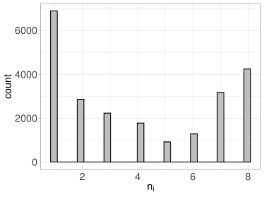
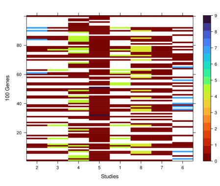
Figure 2: Left: Frequency distribution of the $n_{i}$’s. Right: heatmap of the $\log$ evidence indices for $100$ randomly sampled genes across the $d$ studies. White shade represents a gene not analyzed by the corresponding study while the shade of brown represents an evidence index of $0$ which corresponds to failure to reject.

The sixth column of Table 1 reports the number of rejections for each of these studies and the last column presents the evidence against each rejected null hypothesis in study $j$. It is interesting to see that study 5 (Varambally et al., 2005) receives the highest evidence for its rejected hypotheses, which is not surprising given the large weight $w_{5}$ that each of its relatively small number of rejections receive. In contrast, study 8 (Wallace et al., 2008) has the smallest non-zero evidence which is driven by the largest number of rejections reported in this study. The right panel of Figure 2 presents a heatmap of the $\log$ evidence indices for $100$ randomly sampled genes across the $d$ studies. Here the white shade represents a gene not analyzed by the study while the shade of brown represents an evidence index of $0$ which corresponds to failure to reject the underlying null hypothesis. The heterogeneity across the $d$ studies is evident through the different magnitudes of the evidence indices constructed for each study. Table 2 presents the distribution of the rejected hypotheses across the $d$ studies, with the exception of study 7. For instance, studies 1 and 3 share $1,531$ rejected hypotheses while studies 2 and 5 share just $1$ rejected hypothesis. Also, study 5, which investigates the largest number of genes, has minimal overlap with the other studies as far as its discoveries are concerned.

Table 2: Distribution of rejection overlaps across $7$ studies.

$j$	$\|\bm{\delta}_{j}\|_{0}$	1	2	3	4	5	6	8
1	2,094	-	509	1531	387	7	130	1029
2	921	509	-	423	108	1	27	324
3	1,624	1531	423	-	294	7	105	809
4	3,328	387	108	294	-	17	172	970
5	282	7	1	7	17	-	4	8
6	1,234	130	27	105	172	4	-	365
8	4,716	1029	324	809	970	8	365	-

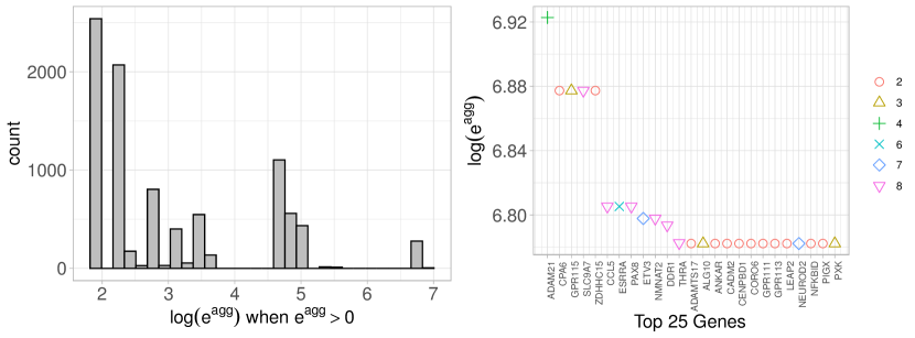
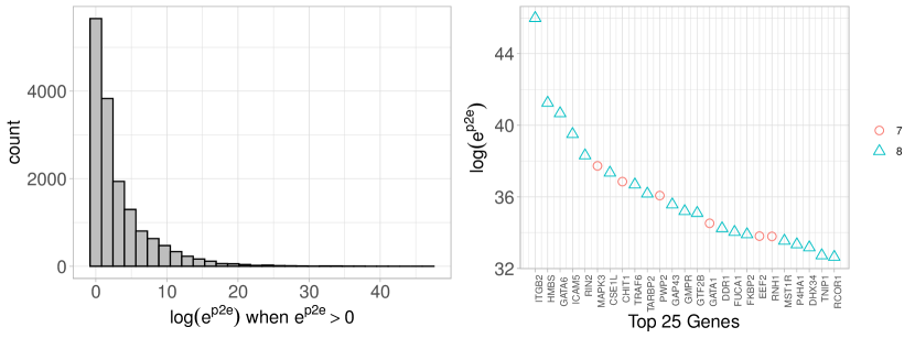
Figure 3: Left: Histogram of the log transformed non-zero aggregated evidences from IRT. Right: Top 25 genes with respect to their aggregated evidence, color and shape-coded by the number of times the corresponding gene was analyzed across the $d$ studies.

Figure 4: Left: histogram of the log transformed non-zero aggregated evidences from P2E. Right: Top 25 genes with respect to their aggregated evidence, color and shape-coded by the number of times the corresponding gene was analyzed across the $d$ studies.

The left panel of Figure 4 presents a histogram of the log transformed non-zero aggregated evidences from IRT while the right panel plots the top 25 genes with respect to their aggregated evidence, colored and shape-coded by the number of times the corresponding gene was analyzed across the $d$ studies. Interestingly, the top second and third genes have $n_{i}=2$ and $3$, respectively, suggesting that apart from the number of times a particular null hypothesis is analyzed across the $d$ studies, the magnitude of the study-specific evidence indices also play a key role in the overall ranking. To put this into perspective, the right panel of Figure 4 presents the top 25 genes with respect to their aggregated evidence from the P2E framework introduced in Section 4.4. In a stark contrast to the IRT framework, here the top 25 genes have $n_{i}>=7$. Furthermore, both the left and right panels of Figure 4 suggest that $e_{i}^{p2e}$ can be substantially larger in magnitude than $e_{i}^{\sf agg}$ particularly when one of the studies rejects the null hypothesis with an astronomically small $p-$value.

Table 3: Distribution of rejected hypotheses with respect to $n_{i}$ at $\alpha=0.1$.

	# Rejections	$n_{i}=1$	2	3	4	5	6	7	8
IRT	2,405	23.91%	2.95%	4.53%	1.25%	5.03%	18.04%	15.13%	29.16%
P2E	4,390	7.15%	7.33%	3.03%	4.26%	3.21%	10.20%	23.07%	41.75%

Table 4: Composition of rejected hypotheses at $\alpha=0.1$

			% Rejected at $\alpha=0.1$
$j$	$\|\bm{\delta}_{j}\|_{0}$	$e_{j}^{+}$	by IRT	by P2E
1	2,094	84.04	30.32	63.08
2	921	955.27	100	57.65
3	1,624	108.36	32.45	71.00
4	3,328	81.60	8.71	51.83
5	282	6,999.29	100	65.25
6	1,234	786.30	100	50.40
7	0	0	-	-
8	4,716	53.81	14.48	51.44

Next, we study the composition of rejected hypotheses from IRT and P2E at $\alpha=0.1$. Table 3 presents the distribution of rejected hypotheses with respect to $n_{i}$ and reinforces the point that for IRT, the evidence weights $w_{j}$ play a key role in the overall ranking while P2E relies on how often a hypothesis has been tested across the $d$ studies. For each study $j$, Table LABEL:tab:realdata2 presents the number of hypotheses rejected by IRT and P2E as a percentage of the total number of rejections for that study. In case of IRT, studies 2, 5, and 6 have a $100\%$ rejection rate which is not surprising given that these three studies also exhibit the three highest evidence against their rejected null hypotheses. Notably, Study 8 has a higher percentage rejection than Study 4 even though the former has a lower evidence index. This is expected since, from Table 2, out of the 4,716 rejected hypotheses in Study 8, approximately $14\%$ are shared with studies 2 and 6, which exhibit high evidence indices. In contrast, of the 3,328 hypotheses rejected in Study 4, less than $8.5\%$ Study 2 and Study 6. Thus, the aggregated evidence index for the rejected hypotheses in Study 8 receive an overall higher weight. In contrast, P2E exhibits a relatively more even distribution of the rejected hypotheses across the $d$ studies which is primarily driven by the magnitude of the $p-$values returned by each study.

6 Numerical experiments

Here we assess the empirical performance of IRT on simulated data. We consider six simulation scenarios with $m=1000$ and test $H_{0i}:\mu_{i}=0~{}vs~{}H_{1i}:\mu_{i}\neq 0$, where $\mu_{i}\stackrel{{\scriptstyle i.i.d.}}{{\sim}}0.8N(0,1)+0.1N(3,1)+0.1N(-3,1)$. In each scenario, study $j$ uses data $X_{ij}$, to be specified subsequently, to conduct $m_{j}$ tests and reports the corresponding decisions $\bm{\delta}_{j}$ obtained from the BH-procedure that controls the FDR at level $\alpha_{j}$. The empirical performance of IRT is compared against three alternative procedures: (1.) the Naive method which rejects $H_{0i}$ if at least $d/2$ studies reject it, (2.) the method Fisher which pools the study specific $p-$values using Fisher’s method (Fisher, 1948) and then applies the BH-procedure on the pooled $p-$value sequence for FDR control, and (3.) the P2E procedure discussed in Section 4.4. When the $p-$values are independent, we expect Fisher to exhibit higher power than $e-$value procedures, such as IRT and P2E. Nevertheless, in such settings Fisher provides a practical benchmark for assessing the empirical performances of P2E, IRT and Naive, where the last two procedures rely only the binary decision sequences $\bm{\delta}_{j}$.
 
Scenario 1 - in this scenario we let $X_{ij}|\mu_{i},\sigma_{j}\stackrel{{\scriptstyle ind.}}{{\sim}}N(\mu_{i},\sigma_{j}^{2}),~{}\sigma_{j}\stackrel{{\scriptstyle i.i.d.}}{{\sim}}U(0.75,2)$, $m_{j}=m$, $\alpha_{j}=0.01$, $\alpha=0.1$ and vary $d$ from $5$ to $50$. Figure 5 presents the average FDP and the ETP across 500 Monte Carlo repetitions. Unsurprisingly, Fisher exhibits the highest power across all values of $d$ while IRT is the next best. The Naive method, on the other hand, is substantially less powerful. While all methods control the FDR at $\alpha$, P2E is less powerful than IRT in this setting. Infact, in all our simulation scenarios, we find that IRT dominates P2E in power at the same FDR level.

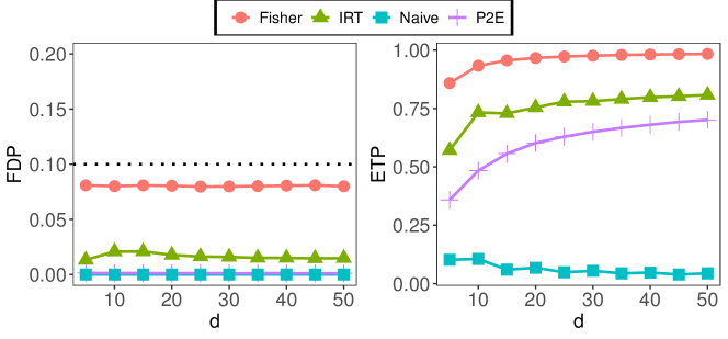
Figure 5: Scenario 1

Scenario 2 - we continue to borrow the setting from Scenario 1 but set $\sigma_{j}=1,~{}d=5$ and introduce correlation across the $d$ studies. Specifically, we let $\text{Corr}(X_{ij},X_{ik})=\rho,~{}j\neq k$ where $\rho\in\{-0.2,-0.1,0,0.1,0.3,0.5,0.7,0.9\}$. In this scenario, the $d$ $p-$values for each hypothesis are exchangeable but not independent unless $\rho=0$. Figure 6 reports the average FDP and the ETP for various methods. Fisher fails to control the FDR at $\alpha=0.1$ for large $\rho$ and therefore does not appear in the left panel of Figure 6. We find that IRT continues to dominate P2E and Naive for all values of $\rho$. Here HM represents another method which pools the study specific $p-$values using harmonic mean (Wilson, 2019) and then applies the BH-procedure on those pooled $p-$values for FDR control. Other methods for pooling exchangeable $p-$values are discussed in Vovk and Wang (2020) but all of them rely on some prior knowledge regarding the strength of the dependence between the $p-$values, which may not be available in practice.

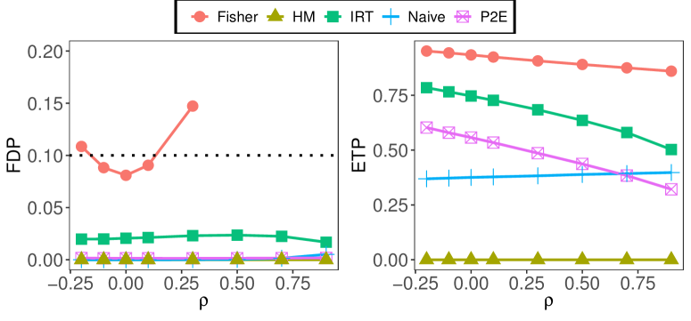
Figure 6: Scenario 2

Scenario 3 - we set $\sigma_{j}=1$ and introduce correlation across the studies as well as the test statistics. Specifically, we let $\text{Corr}(X_{ij},X_{ik})=0.7,~{}j\neq k$ and $\text{Corr}(X_{ij},X_{rj})=0.5,i\neq r$. Figure 7 reports the average FDP and the ETP for various methods as $d$ varies from $5$ to $50$. We see a similar pattern as Figure 6 where IRT controls the FDR and exhibits higher power than Naive, HM and P2E. The results from scenarios 2 and 3 suggest that when the $p-$values are exchangeable, IRT provides a powerful framework for pooling inferences across the various studies. Furthermore, while the building blocks of IRT involve the study-specific binary decision sequences, it is more powerful than P2E which directly relies on the magnitude of study-specific $p-$values for conversion to $e-$values.

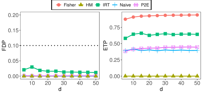
Figure 7: Scenario 3

Scenario 4 - we fix $d=30$ and borrow the setting from Scenario 1 except that for all non-null cases exactly $K$ out of the $d$ studies reject the null hypotheses. Figure 8 reports the average FDP and the ETP for the two methods for different choices of $K$. In this scenario, we expect all methods to exhibit higher power as $K$ increases. The Naive method in, particular, has almost no power for small $K$ while IRT dominates P2E across all values of $K$.

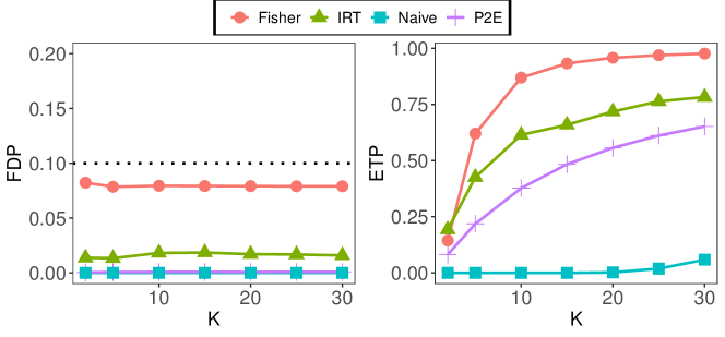
Figure 8: Scenario 4

Scenario 5 - here the data are generated according to Scenario 1 with $\sigma_{j}=1$ but we vary $m_{j}$ for the $d$ studies. Specifically, we set $d=30$, $n=20$ and consider the ratio $\eta=\min\{n_{1},\ldots,n_{m}\}/n$. For a given choice of $\eta$, we first sample $n_{1},\ldots,n_{m}$ uniformly from $[\lceil n\rho\rceil,n]$ with replacement and then for each $i$, $n_{i}$ studies are chosen at random from the $d$ studies without replacement. Figure 9 reports the average FDP and the ETP for the three methods as $\eta$ varies over $[0.05,0.8]$. We also include IRT* and P2E* in our comparisons, which correspond to the IRT and P2E procedures using $\bm{e}^{\sf agg*}$ and $\bm{e}^{p2e*}=(e_{1}^{p2e*},\ldots,e_{m}^{p2e*})$ from Equation (7) and Section 4.4, respectively. As $\eta$ increases, the number of studies testing any given hypothesis $i$ increases, which leads to an improved power for IRT and IRT* in this scenario. Moreover, as discussed in Section 4, IRT* exhibits a higher power than IRT and their power is comparable when the heterogeneity in $n_{i}$ is small, which corresponds to a large value of $\eta$.

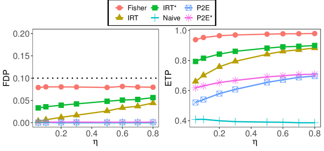
Figure 9: Scenario 5

Scenario 6 - in this scenario we vary $(m_{j},\alpha_{j})$ and continue to include IRT* and P2E* in our comparisons. We borrow the setting from Scenario 1 with $\sigma_{j}=1$, $m=1000$ and $\alpha=0.15$. To vary $m_{j}$, we set $m_{(1)}=\max\{m_{1},\ldots,m_{d}\}=900$ and consider the ratio $\eta=\min\{m_{1},\ldots,m_{d}\}/m_{(1)}$. For a given choice of $\eta$, we first sample $m_{1},\ldots,m_{d}$ uniformly from $[\lceil m_{(1)}\rho\rceil,m_{(1)}]$ with replacement and then for each $j$, $m_{j}$ hypotheses are chosen at random from the $m$ hypotheses without replacement. We set $\alpha_{j}\in\{0.05,0.03,0.01\}$ according to $m_{j}\leq 600$, $m_{j}\in(600,800]$ or $m_{j}>800$, respectively. Thus, in this setting studies with a higher $m_{j}$ receive a larger weight on their rejections. Figure 10 reports the average FDP and the ETP for various methods as $\eta$ varies over $[0.1,0.6]$. As observed in Figure 9, both IRT and IRT* exhibit higher power as $\eta$ increases with the latter dominating IRT in power for relatively smaller values of $\eta$. Furthermore, when $\eta$ is large, $m_{j}$ is large and studies receive a relatively higher weight $w_{j}$ on their rejections which leads to an improved power in this setting.

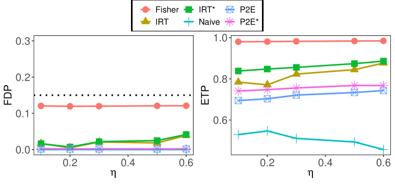
Figure 10: Scenario 6

7 Closing remarks

In this article, we have developed IRT, a framework for fusion learning in multiple testing, that operates on the binary decision sequences available from diverse studies and conducts integrative inference on the common parameter of interest. The IRT framework guarantees an overall FDR control under arbitrary dependence between the aggregated evidence indices as long as the studies control their FDR at the desired levels. Furthermore, our simulation study suggests that IRT provides a powerful approach for pooling exchangeable $p-$values across the studies.

A potential extension of our framework lies in multiple testing of partial conjunction (PC) hypotheses (see Benjamini and Heller (2008); Wang et al. (2022); Bogomolov (2023) for an incomplete list of references) where the goal is to test if at least $u\geq 1$ out of the $d$ studies reject the null hypothesis $H_{0i},~{}i=1,\ldots,m$. This can be formulated as testing the following null hypotheses $H_{0i}^{u/d}:\text{fewer than $u$ out of $d$ studies are non-null}$. Such problems arise in the study of mediation effects (Huang, 2019; Dai et al., 2022; Liu et al., 2022), finding evidence factors in causal inference (Karmakar et al., 2021), and replicability analysis (Heller et al., 2014; Heller and Yekutieli, 2014). Given the triplet $\mathcal{D}_{j}$ from each study, a key challenge in this setting is to construct an aggregation scheme such that the aggregated evidence indices provide an effective ranking of the $m$ PC hypotheses, $H_{01}^{u/d},\ldots,H_{0m}^{u/d}$ and a cutoff along this ranking can be determined for FDR control. Our future research will be directed towards developing such an evidence aggregation scheme.

References

- Barber and Candès (2015) Barber, R. F. and E. J. Candès (2015). Controlling the false discovery rate via knockoffs. The Annals of Statistics 43(5), 2055 – 2085.
- Barrett et al. (2012) Barrett, T., S. E. Wilhite, P. Ledoux, C. Evangelista, I. F. Kim, M. Tomashevsky, K. A. Marshall, K. H. Phillippy, P. M. Sherman, M. Holko, et al. (2012). Ncbi geo: archive for functional genomics data sets—update. Nucleic acids research 41(D1), D991–D995.
- Bashari et al. (2023) Bashari, M., A. Epstein, Y. Romano, and M. Sesia (2023). Derandomized novelty detection with fdr control via conformal e-values. arXiv preprint arXiv:2302.07294.
- Benjamini and Heller (2008) Benjamini, Y. and R. Heller (2008). Screening for partial conjunction hypotheses. Biometrics 64(4), 1215–1222.
- Benjamini and Hochberg (1995) Benjamini, Y. and Y. Hochberg (1995). Controlling the false discovery rate: a practical and powerful approach to multiple testing. Journal of the Royal statistical society: series B (Methodological) 57(1), 289–300.
- Bogomolov (2023) Bogomolov, M. (2023). Testing partial conjunction hypotheses under dependency, with applications to meta-analysis. Electronic Journal of Statistics 17(1), 102–155.
- Candes et al. (2018) Candes, E., Y. Fan, L. Janson, and J. Lv (2018). Panning for gold:‘model-x’knockoffs for high dimensional controlled variable selection. Journal of the Royal Statistical Society Series B: Statistical Methodology 80(3), 551–577.
- Chi et al. (2022) Chi, Z., A. Ramdas, and R. Wang (2022). Multiple testing under negative dependence. arXiv preprint arXiv:2212.09706.
- Chodera et al. (2020) Chodera, J., A. A. Lee, N. London, and F. von Delft (2020). Crowdsourcing drug discovery for pandemics. Nature Chemistry 12(7), 581–581.
- Couzin (2008) Couzin, J. (2008). Whole-genome data not anonymous, challenging assumptions.
- Dai et al. (2022) Dai, C., B. Lin, X. Xing, and J. S. Liu (2022). False discovery rate control via data splitting. Journal of the American Statistical Association, 1–18.
- Dai et al. (2023) Dai, C., B. Lin, X. Xing, and J. S. Liu (2023). A scale-free approach for false discovery rate control in generalized linear models. Journal of the American Statistical Association, 1–15.
- Dai et al. (2022) Dai, J. Y., J. L. Stanford, and M. LeBlanc (2022). A multiple-testing procedure for high-dimensional mediation hypotheses. Journal of the American Statistical Association 117(537), 198–213.
- Fisher (1948) Fisher, R. A. (1948). Combining independent tests of significance. American Statistician, 2–30.
- Grünwald et al. (2023) Grünwald, P., R. de Heide, and W. Koolen (2023). Safe testing. arXiv 1906.07801. Accepted as discussion paper to the Journal of the Royal Statistical Society series B.
- Guo et al. (2023) Guo, Z., X. Li, L. Han, and T. Cai (2023). Robust inference for federated meta-learning. arXiv preprint arXiv:2301.00718.
- Hall and Llinas (1997) Hall, D. L. and J. Llinas (1997). An introduction to multisensor data fusion. Proceedings of the IEEE 85(1), 6–23.
- Heller et al. (2014) Heller, R., M. Bogomolov, and Y. Benjamini (2014). Deciding whether follow-up studies have replicated findings in a preliminary large-scale omics study. Proceedings of the National Academy of Sciences 111(46), 16262–16267.
- Heller and Yekutieli (2014) Heller, R. and D. Yekutieli (2014). Replicability analysis for genome-wide association studies. The Annals of Applied Statistics 8(1), 481 – 498.
- Huang (2019) Huang, Y.-T. (2019). Genome-wide analyses of sparse mediation effects under composite null hypotheses. The Annals of Applied Statistics 13(1), 60 – 84.
- Ignatiadis et al. (2022) Ignatiadis, N., R. Wang, and A. Ramdas (2022). E-values as unnormalized weights in multiple testing. arXiv preprint arXiv:2204.12447.
- Jamoos and Abuawwad (2020) Jamoos, A. and R. Abuawwad (2020). Distributed m-ary hypothesis testing for decision fusion in multiple-input multiple-output wireless sensor networks. IET Communications 14(18), 3256–3260.
- Jiao et al. (2021) Jiao, Y., Y. Wu, and S. Lu (2021). The role of crowdsourcing in product design: The moderating effect of user expertise and network connectivity. Technology in Society 64, 101496.
- Kang et al. (2012) Kang, D. D., E. Sibille, N. Kaminski, and G. C. Tseng (2012). Metaqc: objective quality control and inclusion/exclusion criteria for genomic meta-analysis. Nucleic acids research 40(2), e15–e15.
- Karmakar et al. (2021) Karmakar, B., D. S. Small, and P. R. Rosenbaum (2021). Reinforced designs: Multiple instruments plus control groups as evidence factors in an observational study of the effectiveness of catholic schools. Journal of the American Statistical Association 116(533), 82–92.
- Lapointe et al. (2004) Lapointe, J., C. Li, J. P. Higgins, M. Van De Rijn, E. Bair, K. Montgomery, M. Ferrari, L. Egevad, W. Rayford, U. Bergerheim, et al. (2004). Gene expression profiling identifies clinically relevant subtypes of prostate cancer. Proceedings of the National Academy of Sciences 101(3), 811–816.
- Liu et al. (2022) Liu, D., R. Y. Liu, and M.-g. Xie (2022). Nonparametric fusion learning for multiparameters: Synthesize inferences from diverse sources using data depth and confidence distribution. Journal of the American Statistical Association 117(540), 2086–2104.
- Liu et al. (2021) Liu, M., Y. Xia, K. Cho, and T. Cai (2021). Integrative high dimensional multiple testing with heterogeneity under data sharing constraints. The Journal of Machine Learning Research 22(1), 5607–5632.
- Liu et al. (2022) Liu, Z., J. Shen, R. Barfield, J. Schwartz, A. A. Baccarelli, and X. Lin (2022). Large-scale hypothesis testing for causal mediation effects with applications in genome-wide epigenetic studies. Journal of the American Statistical Association 117(537), 67–81.
- Logan (2020) Logan, W. A. (2020). Crowdsourcing crime control. Tex. L. Rev. 99, 137.
- Nanni et al. (2002) Nanni, S., M. Narducci, L. Della Pietra, F. Moretti, A. Grasselli, P. De Carli, A. Sacchi, A. Pontecorvi, A. Farsetti, et al. (2002). Signaling through estrogen receptors modulates telomerase activity in human prostate cancer. The Journal of clinical investigation 110(2), 219–227.
- Nasirigerdeh et al. (2022) Nasirigerdeh, R., R. Torkzadehmahani, J. Matschinske, T. Frisch, M. List, J. Späth, S. Weiss, U. Völker, E. Pitkänen, D. Heider, et al. (2022). splink: a hybrid federated tool as a robust alternative to meta-analysis in genome-wide association studies. Genome Biology 23(1), 1–24.
- Ramdas et al. (2022) Ramdas, A., P. Grünwald, V. Vovk, and G. Shafer (2022). Game-theoretic statistics and safe anytime-valid inference. arXiv preprint arXiv:2210.01948.
- Ramdas et al. (2020) Ramdas, A., J. Ruf, M. Larsson, and W. Koolen (2020). Admissible anytime-valid sequential inference must rely on nonnegative martingales. arXiv preprint arXiv:2009.03167.
- Ren and Barber (2022) Ren, Z. and R. F. Barber (2022). Derandomized knockoffs: leveraging e-values for false discovery rate control. arXiv preprint arXiv:2205.15461.
- Ritchie et al. (2015) Ritchie, M. E., B. Phipson, D. Wu, Y. Hu, C. W. Law, W. Shi, and G. K. Smyth (2015). limma powers differential expression analyses for rna-sequencing and microarray studies. Nucleic acids research 43(7), e47–e47.
- Rustici et al. (2012) Rustici, G., N. Kolesnikov, M. Brandizi, T. Burdett, M. Dylag, I. Emam, A. Farne, E. Hastings, J. Ison, M. Keays, et al. (2012). Arrayexpress update—trends in database growth and links to data analysis tools. Nucleic acids research 41(D1), D987–D990.
- Shafer (2021) Shafer, G. (2021). Testing by betting: A strategy for statistical and scientific communication. Journal of the Royal Statistical Society Series A: Statistics in Society 184(2), 407–431.
- Shah et al. (2016) Shah, N., Y. Guo, K. V. Wendelsdorf, Y. Lu, R. Sparks, and J. S. Tsang (2016). A crowdsourcing approach for reusing and meta-analyzing gene expression data. Nature biotechnology 34(8), 803–806.
- Shen and Wang (2001) Shen, H. and X. Wang (2001). Multiple hypotheses testing method for distributed multisensor systems. Journal of Intelligent and Robotic Systems 30, 119–141.
- Singh et al. (2002) Singh, D., P. G. Febbo, K. Ross, D. G. Jackson, J. Manola, C. Ladd, P. Tamayo, A. A. Renshaw, A. V. D’Amico, J. P. Richie, et al. (2002). Gene expression correlates of clinical prostate cancer behavior. Cancer cell 1(2), 203–209.
- Storey (2002) Storey, J. D. (2002). A direct approach to false discovery rates. Journal of the Royal Statistical Society: Series B (Statistical Methodology) 64(3), 479–498.
- Sun et al. (2022) Sun, D., T. M. Nguyen, R. J. Allaway, J. Wang, V. Chung, V. Y. Thomas, M. Mason, I. Dimitrovsky, L. Ericson, H. Li, et al. (2022). A crowdsourcing approach to develop machine learning models to quantify radiographic joint damage in rheumatoid arthritis. JAMA network open 5(8), e2227423–e2227423.
- Surowiecki (2005) Surowiecki, J. (2005). The wisdom of crowds. Anchor.
- Tomlins et al. (2005) Tomlins, S. A., D. R. Rhodes, S. Perner, S. M. Dhanasekaran, R. Mehra, X.-W. Sun, S. Varambally, X. Cao, J. Tchinda, R. Kuefer, et al. (2005). Recurrent fusion of tmprss2 and ets transcription factor genes in prostate cancer. science 310(5748), 644–648.
- Varambally et al. (2005) Varambally, S., J. Yu, B. Laxman, D. R. Rhodes, R. Mehra, S. A. Tomlins, R. B. Shah, U. Chandran, F. A. Monzon, M. J. Becich, et al. (2005). Integrative genomic and proteomic analysis of prostate cancer reveals signatures of metastatic progression. Cancer cell 8(5), 393–406.
- Vovk and Wang (2020) Vovk, V. and R. Wang (2020). Combining p-values via averaging. Biometrika 107(4), 791–808.
- Vovk and Wang (2021) Vovk, V. and R. Wang (2021). E-values: Calibration, combination and applications. The Annals of Statistics 49(3), 1736–1754.
- Vovk and Wang (2023) Vovk, V. and R. Wang (2023). Confidence and discoveries with e-values. Statistical Science 38(2), 329–354.
- Wallace et al. (2008) Wallace, T. A., R. L. Prueitt, M. Yi, T. M. Howe, J. W. Gillespie, H. G. Yfantis, R. M. Stephens, N. E. Caporaso, C. A. Loffredo, and S. Ambs (2008). Tumor immunobiological differences in prostate cancer between african-american and european-american men. Cancer research 68(3), 927–936.
- Wang et al. (2022) Wang, J., L. Gui, W. J. Su, C. Sabatti, and A. B. Owen (2022). Detecting multiple replicating signals using adaptive filtering procedures. The Annals of Statistics 50(4), 1890 – 1909.
- Wang and Ramdas (2022) Wang, R. and A. Ramdas (2022). False discovery rate control with e-values. Journal of the Royal Statistical Society Series B: Statistical Methodology 84(3), 822–852.
- Wasserman et al. (2020) Wasserman, L., A. Ramdas, and S. Balakrishnan (2020). Universal inference. Proceedings of the National Academy of Sciences 117(29), 16880–16890.
- Welsh et al. (2001) Welsh, J. B., L. M. Sapinoso, A. I. Su, S. G. Kern, J. Wang-Rodriguez, C. A. Moskaluk, H. F. Frierson Jr, and G. M. Hampton (2001). Analysis of gene expression identifies candidate markers and pharmacological targets in prostate cancer. Cancer research 61(16), 5974–5978.
- Wilson (2019) Wilson, D. J. (2019). The harmonic mean p-value for combining dependent tests. Proceedings of the National Academy of Sciences 116(4), 1195–1200.
- Wolfson et al. (2010) Wolfson, M., S. E. Wallace, N. Masca, G. Rowe, N. A. Sheehan, V. Ferretti, P. LaFlamme, M. D. Tobin, J. Macleod, J. Little, et al. (2010). Datashield: resolving a conflict in contemporary bioscience—performing a pooled analysis of individual-level data without sharing the data. International journal of epidemiology 39(5), 1372–1382.
- Xu and Ramdas (2023) Xu, Z. and A. Ramdas (2023). More powerful multiple testing under dependence via randomization. arXiv preprint arXiv:2305.11126.
- Yu et al. (2004) Yu, Y. P., D. Landsittel, L. Jing, J. Nelson, B. Ren, L. Liu, C. McDonald, R. Thomas, R. Dhir, S. Finkelstein, et al. (2004). Gene expression alterations in prostate cancer predicting tumor aggression and preceding development of malignancy. Journal of clinical oncology 22(14), 2790–2799.
- Zerhouni and Nabel (2008) Zerhouni, E. A. and E. G. Nabel (2008). Protecting aggregate genomic data. Science 322(5898), 44–44.