Abstract

We show that by allowing our Universe to merge with other universes one is lead to modified Friedmann equations that explain the present accelerated expansion of our Universe without the need of a cosmological constant.

1 Introduction

We have proposed a modified Friedmann equation [1, 2] which changes the late time cosmology, such that one does not need a cosmological constant to explain the present day acceleration of our Universe. While it is our hope that this modified Friedmann equation can eventually be derived from an underlying microscopic theory [3], we will here treat it as a phenomenological model that we can obtain in a simple way from the standard Friedmann equation.

Our starting point is the Hartle-Hawking minisuperspace action, which after the rotation of the conformal factor can be written as

$$S=\int dt\,\Big{(}\frac{\beta\dot{v}^{2}}{2Nv}+\lambda Nv\Big{)}.$$ (1)

Before rotating to Euclidean spacetime and the rotation of the conformal factor, this action is just the standard minisuperspace action

$$S=\int dt\,\Big{(}-\frac{\beta\dot{v}^{2}}{2Nv}-\lambda Nv\Big{)},$$ (2)

written using the metric

$$ds^{2}=-N^{2}(t)dt^{2}+a^{2}(t)d\Omega_{d},\qquad d\Omega_{d}=\sum_{i=1}^{d}dx_{i}^{2}.$$ (3)

In (1) and (2) we are using units where $c=\hbar=1$ and the constant $\beta=(d-1)/d$, where $d$ is the dimension of space. We have used

$$v(t)=\frac{1}{\kappa}a^{d}(t),\quad\kappa=8\pi G,\quad\mbox{$G=$ the gravitational constant.}$$ (4)

as variable rather than the scale factor $a(t)$. $v(t)$ is proportional to the spatial $d$-volume at time $t$ and below we will just call it the $d$-volume. For the Hubble parameter $H(t)$ we then have

$$H(t)\equiv\frac{\dot{a}}{a}=\frac{1}{d}\,\frac{\dot{v}}{v}.$$ (5)

The reason we prefer to use $v(t)$ instead of $a(t)$ is that the minisuperspace action (1)-(2) is then valid in all space dimensions $d>1$. Finally $\lambda$ denotes the cosmological constant. Presently we will ignore matter, only assume a cosmological constant term. Below we will include matter in our considerations.

It should be noted that (1) also appears as the leading term in an effective action in a model of four-dimensional quantum gravity known as Causal Dynamical Triangulations (CDT). In that case one is not assuming a minisuperspace reduction, but performs the path integral over all degrees of freedom except $v(t)$. Thus (1) might be more general than suggested by the minisuperspace reduction. This CDT result is a numerical result, obtained via Monte Carlo Simulations of the CDT lattice gravity model where one identifies $G/\varepsilon^{2}$ and $\lambda\varepsilon^{4}$ with the corresponding dimensionless lattice coupling constants, $\varepsilon$ denoting the length of the lattice links, i.e. the UV lattice cut-off (see [5], and [6] for reviews). Quite remarkably, for CDT in $d=1$, (1) can be derived analytically (with $\beta\neq 0$), and it is an effective action coming entirely from the path integral measure [7], since the classical Einstein action is a topological invariant in the case of $d=1$.

The classical Hamiltonian corresponding to (2) is

$${\cal H}(v,p)=Nv\Big{(}-\frac{p^{2}}{2\beta}+\lambda\Big{)},$$ (6)

where $p$ denotes the momentum conjugate to $v$. In the following we will be interested in $d=3$, i.e. $2\beta=4/3$.

A classical solution corresponding to the action (2) is the de Sitter spacetime

$$v(t)=v(t_{0})\,{\rm e}^{\sqrt{3\lambda}(t-t_{0})}.$$ (7)

We now want to go beyond this classical picture, but staying as close as possible to the minisuperspace picture, by trying to include the possibility that our Universe can absorb other universes, which we denote baby universes even if they are not necessarily small.

2 Expansion by merging with other universes

Since we will allow for other universes to merge with our Universe, we are really discussing a multi-universe theory and like in a many-particle theory it is natural to introduce creation and annihilation operators $\Psi^{\dagger}(v)$ and $\Psi(v)$ for single universes of spatial volume $v$. In a full theory of four-dimensional quantum gravity the spatial volume alone will of course not provide a complete characterization of a state at a given time $t$. As mentioned we will here make the drastic simplification to work in a minisuperspace approximation where the spatial universe is characterized entirely by the spatial volume $v$. Thus, denote the quantum state of a spatial universe with volume $v$ by $|v\rangle$. We consider now the multi-universe Fock space constructed from such single universe states and denote the Fock vacuum state by $|0\rangle$. Then

$$[\Psi(v),\Psi^{\dagger}(v^{\prime})]=\delta(v-v^{\prime}),\quad\Psi^{\dagger}(v)|0\rangle=|v\rangle,\quad\Psi(v)|0\rangle=0.$$ (8)

In this way the (minisuperspace) quantum Hamiltonian that includes the creation and destruction of universes can be written as [8]

$${\hat{H}} = {\hat{H}}^{(0)}-g\int dv_{1}\int dv_{2}\;\Psi^{\dagger}(v_{1})\Psi^{\dagger}(v_{2})\;(v_{1}\!+\!v_{2})\Psi(v_{1}\!+\!v_{2})-$$

$$\!\!\!g\int dv_{1}\int dv_{2}\;\Psi^{\dagger}(v_{1}\!+\!v_{2})\;v_{2}\Psi(v_{2})\;v_{1}\Psi(v_{1})-\!\int\frac{dv}{v}\,\rho(v)\Psi^{\dagger}(v),\quad\rho(v)=\delta(v)$$

$${\hat{H}}^{(0)}=\int_{0}^{\infty}\frac{dv}{v}\;\Psi^{\dagger}(v)\hat{{\cal H}}^{(0)}\,v\Psi(v),~{}~{}~{}~{}~{}\hat{{\cal H}}^{(0)}={v}\Big{(}-\frac{3}{4}\frac{d^{2}}{dv^{2}}\,+\lambda\Big{)}$$ (10)

${{\hat{H}}}^{(0)}$ describes the quantum Hamiltonian corresponding to the action (1) (with $\beta=2/3$) and describes the propagation of a single universe, while the two cubic terms describe the splitting of a universe into two and the merging of two universes into one, respectively. Finally, the last term implies that a universe can be created from the Fock vacuum $|0\rangle$ provided the spatial volume is zero. If it was not for this term ${\hat{H}}|0\rangle=0$, and the Fock vacuum would be stable. Again, in our minisuperspace approximation we do not attempt to describe how such a merging or splitting realistically takes place, the only thing which has our interest is how the volume of space can be influenced by such merging or splitting processes, and for this the minisuperspace model might give us some interesting hints.

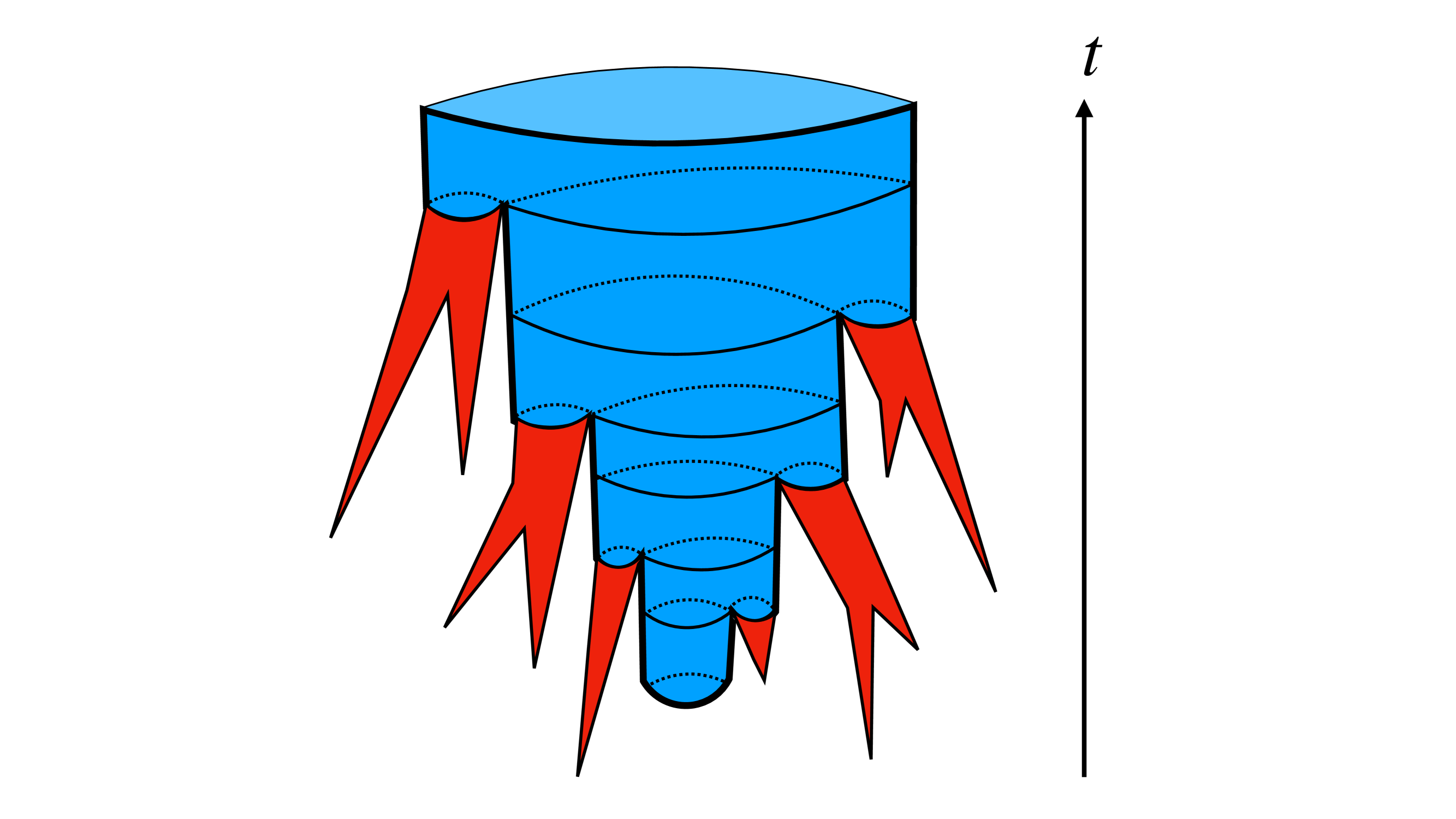
Even the minisuperspace Hamiltonian ${\hat{H}}$ is too complicated to be solved in general. A universe can successively split in many, be joined by many and a part that splits off can later rejoin, thereby changing the topology of spacetime. Since the Hamiltonian is essentially dimension independent (all dimension dependence is absorbed in the coupling constants $\kappa$, $\lambda$ and $g$), what we are describing is the so-called string field theory of two-dimensional CDT [8]. For this string field theory there exists a truncation that can be solved analytically [9], called generalized CDT (GDCT), and that at the same time has our main interest from a cosmological point of view. It follows the evolution of a universe (let us call it “our” Universe) in time. During this evolution it can merge with other universes (denoted baby universes), created at times $t_{i}$ with spatial volumes $v_{i}(t_{i})=0$ (see Fig. 1). We will assume these universes have the same coupling constants as our Universe. The effective Hamiltonian, the so-called inclusive Hamiltonian, first introduced in [11], governing the evolution of the Universe, is obtained from the path integral by integrating over the times $t_{i}$ and summing over the number of baby universes merging with our Universe. In the path integral, the various baby universes, characterized at a given time $t$ by spatial volumes $v_{i}(t)$, can themselves be merged with other baby universes. One integrates over all possible $v_{i}(t)$, not necessarily related to solutions of any classical equations.

Figure 1: Our Universe (blue), represented as one-dimensional circles, propagating in time, with baby universes (red) merging and increasing the spatial volume.

Let us describe in some detail how such an inclusive Hamiltonian can be obtained from ${\hat{H}}$. The simplest way to incorporate an absorption of baby universes into the propagation of our Universe is to replace the quantum field $\Psi(v)$, representing the disappearance of a universe of spatial volume $v$ when it is absorbed by our Universe, by a classical field $\psi(v)$. Thus we make the following replacement in the third term on the rhs of eq. (2)

$$\Psi^{\dagger}(v_{1}+v_{2})\Psi(v_{1})\Psi(v_{2})\to\Psi^{\dagger}(v_{1}+v_{2})\psi(v_{1})\Psi(v_{2})+\Psi^{\dagger}(v_{1}+v_{2})\Psi(v_{1})\psi(v_{2})$$ (11)

The terms on the rhs of eq. (11) contribute to the propagation of our Universe since they are of the form $\Psi^{\dagger}(v_{1})\big{(}\cdot\big{)}\Psi(v_{2})$, but contrary to the terms in ${\hat{H}}_{0}$ they are non-local in $v$. By Taylor expanding $\Psi^{\dagger}(v+w)$ around $v$, this non-locality can be expanded as a power series in the non-local operator $(d/dv)^{-1}$. After some algebra this leads to

$$\int dvdw\,\Psi^{\dagger}(v+w)\,w\psi(w)\,v\Psi(v)=\int dv\Psi^{\dagger}(v)\,F\!\left(\frac{d}{dv}\right)v\Psi(v),$$ (12)

where $F(p)$ is the Laplace transform of $\phi(v)=v\psi(v)$:

$$\phi(v)=\phi_{0}+\phi_{1}{v}+\phi_{2}{v^{2}}+\cdots,\quad F(p)=\int_{0}^{\infty}\!\!\!dv\;{\rm e}^{-p\,v}\phi(v)=\frac{\Gamma(1)\phi_{0}}{p}+\frac{\Gamma(2)\phi_{1}}{p^{2}}+\cdots$$ (13)

Thus $\hat{{\cal H}}_{0}$ from (10) will be replaced by the inclusive Hamiltonian

$$\hat{{\cal H}}_{\rm inc}=\hat{{\cal H}}_{0}-2gF\!\left(\frac{d}{dv}\right){v}$$ (14)

In GCDT $F(p)$ is determined by the self-consistency requirement that our Universe, modified by the impact $\phi(v)$ of baby universes, should be identical to the baby universes it absorbs. We refer to [9] (or to the Lecture Notes [12] ) for the details of this determination. Finally, rotating back from the Hartle-Hawking metric to Lorentzian signature, as when going from (1) to (2) and replacing the $-id/dv$ by the classical momentum $p$ conjugate to $v$ we obtain the following semiclassical Hamiltonian

$${\cal H}={v}\Big{(}-\,\frac{3}{4}(p^{2}+{\lambda}-2gF(p)\Big{)}=\frac{3}{4}{v}\Big{(}(p+\alpha)\sqrt{(p-\alpha)^{2}+\frac{2g}{\alpha}}\;\;\Big{)},$$ (15)

where $\alpha$ satisfies the equation

$$\alpha^{3}-\frac{4}{3}\lambda\alpha-g=0,$$ (16)

It is seen that if $g=0$ one obtains precisely the $H$ in (6) (with $N=1$). A solution to the “on shell” Hamiltonian equations is

$$v(t)=v(t_{0})\,{\rm e}^{\frac{3}{2}\Sigma(t-t_{0})},\quad\Sigma=\sqrt{\alpha^{2}+\frac{g}{2\alpha}}.$$ (17)

Again, if we choose $g\!=\!0$ we obtain the de Sitter solution (7). Increasing $g$ will increase the expansion rate of the universe, the intuition behind this being illustrated in Fig. 1, and we can actually take the cosmological constant $\lambda\!=\!0$ and still obtain an expanding universe:

$$v(t)=v(t_{0})\,{\rm e}^{\sqrt{\frac{27}{8}}\,g^{1/3}(t-t_{0})}.$$ (18)

Thus we have the same classical de Sitter solution as (7) provided

$$g^{2/3}=\frac{8}{9}\;\lambda,$$ (19)

but the origin of this exponential expansion is now not a cosmological constant but instead the “bombardment” of our Universe by baby universes.

3 Including matter

Until now we have considered our Universe, but without matter. We will now include matter in the most simple way, as a matter density $\rho_{\rm m}(v)$ in the Hamiltonian (15). In addition we will only consider relatively late times in the evolution of our universe, namely the period after the time of last scattering ($t_{\rm LS}$), where matter to a good approximation can be considered as dust that exerts zero pressure . Thus the Hamiltonian has the form

$${\cal H}[v,p]={v}\,(-f(p)+\kappa\rho_{\rm m}(v)\,),\quad v\rho_{\rm m}(v)=v_{0}\rho_{\rm m}(v_{0}),$$ (20)

where $v_{0}$ and $\rho_{\rm m}(v_{0})$ denote the values at the present time $t_{0}$ and where we will later consider three different choices of $f(p)$. Before that, let us discuss the solution of the eoms for arbitrary $f(p)$ in (20). The eoms simplify since $v\rho_{\rm m}(v)$ is constant.

$$\dot{v}=\frac{\partial{\cal H}}{\partial p}=-vf^{\prime}(p),\quad{\rm i.e.}\quad 3\,\frac{\dot{a}}{a}=\frac{\dot{v}}{v}=-f^{\prime}(p)$$ (21)

$$~{}~{}\dot{p}=-\frac{\partial{\cal H}}{\partial v}=f(p),\quad{\rm i.e.}\quad t-t_{\rm LS}=\int_{p_{\rm LS}}^{p}\frac{d\,p}{f(p)}$$ (22)

By construction any solution to (21)-(22) will satisfy ${\cal H}={\rm const}$, and we are interested in the “on-shell” solutions ${\cal H}=0$, which by (20) implies that

$$f(p)=\kappa\rho_{\rm m}(v)=\kappa\rho_{\rm m}(v_{0})\frac{v_{0}}{v}=f(p_{0})\frac{v_{0}}{v}=f(p_{0})(1+z)^{3},$$ (23)

where $p_{0}$ denotes the value of $p$ at present time $t_{0}$ and $z$ denotes the redshift at time $t$, i.e.

$$z(t)+1=\frac{a(t_{0})}{a(t)}=\Big{(}\frac{v(t_{0})}{v(t)}\Big{)}^{1/3}.$$ (24)

Eq. (23) is the generalized Friedmann when eq. (21) is used to express $p$ in terms of ${\dot{a}}/{a}$.

Using $p$ as a parameter instead of $t$ (the relation between the two parameters is defined by eq. (22)) we can immediately write parametric expressions for a number of relevant functions expressed in terms of $f(p)$. Let us define these. The redshift $z(t)$ or $z(p)$ is

$$z=\frac{a(t_{0})}{a(t)}-1=\Big{(}\frac{f(p)}{f(p_{0})}\Big{)}^{\frac{1}{3}}\!\!-1.$$ (25)

The Hubble parameter $H(t)$ or $H(p)$ is defined as (see also eq. (5))

$$H=\frac{\dot{a}(t)}{a(t)}=-\,\frac{1}{3}\,f^{\prime}(p).$$ (26)

The formal density $\rho_{f}(t)$ or $\rho_{f}(p)$ related to the function $f(p)$ is obtained by writing the generalized Friedmann equation (23) as

$$\Big{(}\frac{\dot{a}(t)}{a(t)}\Big{)}^{2}=\frac{\kappa\rho_{\rm m}(v)}{3}+\frac{\kappa\rho_{f}(v)}{3}$$ (27)

from which we deduce (using the eoms)

$$\kappa\rho_{f}(p)=\frac{1}{3}\big{(}f^{\prime}(p)\big{)}^{2}-f(p).$$ (28)

$$\kappa\frac{d{\rho}_{f}}{dt}=f(p)f^{\prime}(p)\Big{(}\frac{2}{3}f^{\prime\prime}(p)-1\Big{)}.$$ (29)

We define the formal pressure $P_{f}$ related to $\rho_{f}$ by the energy conservation equation

$$\frac{d}{dt}(v\rho_{f})+P_{f}\frac{d}{dt}v=0.$$ (30)

This leads to

$$P_{f}=f(p)\Big{(}\frac{2}{3}f^{\prime\prime}(p)-1\Big{)}-\rho_{f}(v)$$ (31)

and the formal equation of state parameter $w_{f}$ is defined (for $\rho_{f}\neq 0$) by

$$w_{f}=\frac{P_{f}}{\rho_{f}}=\frac{f(p)\Big{(}\frac{2}{3}f^{\prime\prime}(p)-1\Big{)}}{\frac{1}{3}\big{(}f^{\prime}(p)\big{)}^{2}-f(p)}-1$$ (32)

The definitions of $\rho_{f}$ and $P_{f}$ ensure that our eoms can be written in the standard GR form, expressed in terms of $a$, $\rho_{\rm m}$, $\rho_{f}$ and $P$.

Finally, we will need the standard definitions of some cosmological distances. $D_{H}$ is defined as the inverse Hubble parameter

$$D_{H}=\frac{1}{H}=-\frac{3}{f^{\prime}(p)}$$ (33)

while

$$D_{M}=\int_{0}^{z}\frac{dz^{\prime}}{H(z^{\prime})}=\int^{t_{0}}_{t}dt^{\prime}\;\frac{a(t_{0})}{a(t)}=\int^{p}_{p_{0}}\frac{dp}{f(p_{0})}\;\Big{(}\frac{f(p_{0})}{f(p)}\Big{)}^{2/3}$$ (34)

and

$$D_{V}=\sqrt[3]{zD_{H}D_{M}^{2}}.$$ (35)

represents a kind of average of the various distances and the so-called angular diameter is often defined as

$$\theta=\frac{r_{s}}{D_{V}},$$ (36)

where $r_{s}$ is the co-moving sound horizon at $t_{\rm drag}$. $\theta$ is an important variable, e.g. in the observations of baryon acoustic oscillations (BAO). Since the physics associated with these oscillations takes place before $t_{\rm LS}$ and thus $t_{\rm drag}<t_{\rm LS}$, $r_{s}$ will be independent of the functions $f$ we consider, for reasons to be discussed below.

In these formulas the coupling constants $\kappa$, $\lambda$ and $g$ are so far arbitrary, and so are $t_{0}$ and $t_{\rm LS}$ (or equivalently, via (22)) $p_{0}$ and $p_{\rm LS}$). If we from observations are given $H_{0}$, the Hubble parameter at present time $t_{0}$, and $z_{\rm LS}$, the redshift at the time of last scattering $t_{\rm LS}$, we can determine $p_{0}$ and $p_{\rm LS}$:

$$f^{\prime}(p_{0})=-3\,H_{0},\quad f(p_{\rm LS})=f(p_{0})(1+z_{\rm LS})^{3}.$$ (37)

This finally leads to the determination of $t_{0}-t_{\rm LS}$ by eq. (22). We need more (experimental) input to determine the coupling constants that enter in $f(p)$. We will discuss this in the next section.

Let us now consider the three choices of $f(p)$ in (20), where $f(p)$ is given by (15). The first choice corresponds to $g=0$, $\lambda>0$:

$$f_{\rm ds}(p)=\frac{3}{4}\,p^{2}-\lambda.$$ (38)

This is of course just the $f(p)$ associated with the standard de Sitter Hamiltonian (6). We include this choice in order to compare the late time cosmology of the standard $\Lambda$CDM model with the results from our new cosmological models. The second choice corresponds to $\lambda=0$ and $g>0$. Thus

$$f_{\rm gcdt}(p)=\frac{3}{4}\,(p+\alpha)\sqrt{(p-\alpha)^{2}+2\alpha^{2}},\qquad\alpha=g^{1/3}.$$ (39)

This is our model where baby universes of any size $v$ can merge with our Universe. The third choice is motivated by expanding $f_{\rm gcdt}(p)$ in powers of $\alpha/p$:

$$f_{\rm gcdt}(p)=\frac{3}{4}\left(p^{2}+\alpha^{2}\left(\frac{2\alpha}{p}+O\Big{(}\frac{\alpha^{2}}{p^{2}}\Big{)}\right)\right)$$ (40)

At early times, $v(t)$ becomes small and according to (20) $\rho(v(t))$ will be large. Thus ${\cal H}(v,p)=0$ implies that $|p|$ is large at early times (i.e. times larger than but close to $t_{\rm LS}$). In addition we expect that in our Universe $g$ is small according to (19). Thus we expect that keeping only the first term in the expansion (40) is a good approximation except at quite late times where the exponential expansion will dominate and where $|p|$ is close to $g^{1/3}$, and this was one of the reasons we in earlier work considered this approximation, which when inserted in (23) led to what we denoted the modified Friedmann equation. We thus define this $f(p)$ as follows

$$f_{\rm mod}(p)=\frac{3}{4}\,\left(p^{2}+\frac{2g}{p}\right).$$ (41)

The last term in (41) is effectively a time dependent cosmological constant. At very late time, when the matter term $\rho(v)\propto 1/v$ plays no role, the modified Friedmann equation implies that $p=-(2g)^{1/3}$ and the term acts precisely as a cosmological constant, as already shown in (18), and in analogy with the $-\lambda$ term in (38). However, for smaller $t$, $|p|$ will increase, as discussed above, and the last term in (41) will be less important.

The three functions $f_{\rm ds}$, $f_{\rm mod}$ and $f_{\rm mod}$ are so simple that even the integrals appearing in (22) and (34) can be expressed as known analytic functions and in this sense the models are fully solvable. In an Appendix we present some details and point out a curious symmetry of the $f_{\rm mod}$-model.

Returning to the expansion (13) that defined the inclusive Hamiltonian, it is seen that the approximation (41) corresponds to $\phi(v)=\phi_{0}+O(v)$, i.e. to the absorption of baby universes of infinitesimal size (which is one reason we introduced the word “baby universe” for the universes absorbed by our Universe). The absorption of such small baby universes can only result in a change of the spatial volume if infinitely many are absorbed per unit time and unit spatial volume.

4 Comparison of the different models

In the three models we introduced above there are two coupling constants. The gravitational coupling constant $\kappa$ is fixed by local experiments and we will not discuss it any further. $f_{\rm ds}(p)$ has the cosmological coupling constant $\lambda$ as a parameter, while $f_{\rm mod}(p)$ and $f_{\rm gcdt}(p)$ have the universe-merging coupling constant $g$ as parameter. $\lambda$ or $g$ are actually determined already from the values $H_{0}$ and $z_{\rm LS}$ mentioned above provided we can assume they play no role for $t<t_{\rm LS}$. We know this is true for $\lambda$ in the $\Lambda$CDM model and from (19), which is of course not exactly true when we add matter to the model, we nevertheless expect that it is also true for $g$ in the other models. This implies that

$$f(p)\approx\frac{3}{4}\,p^{2}\quad{\rm for}\quad 0<t<t_{\rm LS}.$$ (42)

That being the case, we can calculate $t_{\rm LS}$ as well as the relation between $t_{\rm LS}$ and $p_{\rm LS}$ without reference to the specific models. For the purpose of illustration, assume (incorrectly) that we can ignore the radiation density $\rho_{\rm r}(t)$ all the way down to $t\approx 0$. Eq. (22) then leads to

$$t_{\rm LS}=\int_{-\infty}^{p_{\rm LS}}\frac{dp}{\frac{3}{4}\,p^{2}}=-\frac{4}{3}\,\frac{1}{p_{\rm LS}}.$$ (43)

Eqs. (37) determine our coupling constant since the first equation determines $p_{0}$ and the last equation (the generalized Friedmann equation at $t_{\rm LS}$) can be written as

$$f(p_{0})=\frac{3\,p_{\rm LS}^{2}}{4\,(1+z_{\rm LS})^{3}}$$ (44)

So given $t_{\rm LS}$, and thus $p_{\rm LS}$, we can determine either $\lambda$ from $f_{\rm ds}(p)$, or $g$ from $f_{\rm mod}(p)$ or $f_{\rm gcdt}(p)$.

The $t_{\rm LS}$ used in cosmology is obtained by also including the radiation density. In this case we obtain an additional term in eq. (22) from $\partial H/\partial v$ and

$$t_{\rm LS}=\int_{-\infty}^{p_{LS}}\frac{dp}{\frac{3}{4}\,p^{2}+\frac{1}{3}\,\kappa\rho_{\rm r}(v(p))},\qquad\frac{3}{4}\,p^{2}=\kappa\rho_{\rm m}(v)+\kappa\rho_{\rm r}(v).$$ (45)

This $t_{\rm LS}$ is smaller than the one given in (43) and leads to a somewhat different $p_{\rm LS}$, which we should use in (44) to determine the coupling constants. We can effectively compensate for the smaller $t_{\rm LS}$ by shifting the origin of time.

Having determined the coupling constants we can now compare the different models for given $H_{0}$ and $z_{\rm LS}$. While $z_{\rm LS}$ is fixed (almost) model independent to 1090, there are presently two values of $H_{0}$ that do not agree within $5\sigma$ (a fact that is denoted the $H_{0}$ tension). One value is deduced from “local” measurements, using various space candle techniques [13]. We denote it $H_{0}^{\rm SC}$. This value ($H_{0}^{\rm SC}=73.04\pm 1.04$ km/s/Mpc) is almost independent of cosmological models. The other value is deduced from the CMB data created at $t_{\rm LS}$. It is using cosmological models in a number of ways, among those to extrapolate to present time $t_{0}$. This value [14] ($H_{0}^{\rm CMB}=67.4\pm 0.5$ km/s/Mpc), which we denote $H_{0}^{\rm CMB}$, is model dependent and the value usually referred to is based on the $\Lambda$CDM model.

Figure 2: $a(z)H(z)=H(z)/(1+z)$ shown for the three models for $H_{0}=73.0$ (case A). We have included in red the error bars around this point, corresponding to $z=0$, but the curves all start at 73.0. The orange curve corresponds to $f_{\rm ds}$, the red curve to $f_{\rm gcdt}$ and the blue curve to $f_{\rm mod}$. In case B the three models all start at $H_{0}=67.4$, the value suggested by the Planck Collaboration. The green curve corresponds to $f_{\rm ds}$, the dashed red curve to $f_{\rm gcdt}$ and the dashed blue curve to $f_{\rm mod}$. Inserted in red are data from $0<z<3$: the first three points from the baryon acoustic oscillation data [15], the next from quasars [16] and the last two data points from Ly–$\alpha$ measuments [17, 18]

When comparing our two models with the $\Lambda$CDM model we will only use the CMB data to determine $T_{0}$, the temperature of the microwave background radiation at the present time. We have not attempted to use the wealth of information contained in the CMB temperature fluctuations since it requires the use of metric perturbations and it is presently not clear how to incorporate such perturbations in our extended models. We will simply present some of the variables we listed in the previous Section, namely $H(z)$, $D_{V}(z)$ and $w_{f}(z)$, and $t_{0}$, calculated for the three cosmological models, in two cases, namely for $(H_{0}^{\rm SC},z_{\rm LS})$ (case A) and for $(H_{0}^{\rm CMB},z_{\rm LS})$ (case B). For $H(z)$ and $D_{V}(z)$ we can also compare with measurements from which one can extract these observables for relatively low values of $z$.

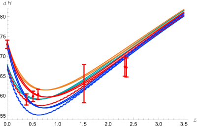
In Fig. 2 we have shown $a(z)H(z)=H(z)/(1+z)$ in case A and B for the three models. It is seen that in case A the $f_{\rm gcdt}$ and the $f_{\rm mod}$ models fit the data better than the $f_{\rm ds}$ model (the $\Lambda$CDM model), while in case B the opposite is the case. Of course we do not know yet whether $H_{0}^{\rm SC}$ or $H_{0}^{\rm CMB}$ is the correct $H_{0}$ value, but if $H_{0}^{\rm SC}$ turns out to be the correct value the $f_{\rm gcdt}$ and the $f_{\rm mod}$ models seems a better choice for the data presented here. Of course there are many other data to take into account if one wants to make a multi-parameter fit, but as already remarked most these data should be matched to the cosmological model using perturbation expansions not yet available for the $f_{\rm gcdt}$ and $f_{\rm mod}$ models. In Table 1 we have listed the reduced $\chi^{2}$ values just calculated from the data and the corresponding error bars shown in Fig. 2 in Case A and B.

	$\chi_{\rm red}$(ds)	$\chi_{\rm red}$(gcdt)	$\chi_{\rm red}$(mod)
case A	3.5	1.5	1.8
case B	1.2	1.7	5.6

Table 1.

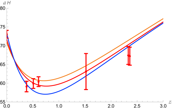
Fig. 3 shows $D_{V}(z)/r_{s}$ for the $f_{\rm ds}$, $f_{\rm gcdt}$ and $f_{\rm mod}$ models, normalized by $(D_{V}(z)/r_{s})^{\rm CMB}$, i.e. the $D_{V}(z)/r_{s}$ for the $f_{\rm ds}$ model in case B.

Figure 3: The three curves starting at value 1 for $z=0$ are curves of $(D_{V}^{f}(z)/r_{s})/(D_{V}^{f_{\rm ds}}(z)/r_{s})^{\rm CMB}$ for the models with $f=f_{\rm gcdt}$ (red, dotted), $f_{\rm mod}$ (blue, dotted) and $f_{\rm ds}$ (green), all for the chosen value $H_{0}=H_{0}^{\rm CMB}$ (case B). The last curve is of course 1, except for the error bars reflecting the uncertainty of $H_{0}^{\rm CMB}$. The three curves starting at value 0.94 for $z=0$ are the curves for $f=f_{\rm gcdt}$ (red), $f_{\rm mod}$ (blue) and $f_{\rm ds}$ (orange), all for $H_{0}=H_{0}^{\rm SC}$ (case A), and again normalized by $(D_{V}^{f_{\rm ds}}(z)/r_{s})^{\rm CMB}$. The data points and error bars are obtained from various BAO surveys (see [2] for a detailed table).

We see here the same trend as in Fig. 2: the $f_{\rm gcdt}$ and the $f_{\rm mod}$ models fit the data better in case A, while the $f_{\rm ds}$-model fits better in case B. In Table 2 we list the reduced $\chi^{2}$ values obtained from Fig. 3:

	$\chi_{\rm red}$(ds)	$\chi_{\rm red}$(gcdt)	$\chi_{\rm red}$(mod)
case A	4.7	2.1	1.0
case B	1.6	4.1	13.7

Table 2.

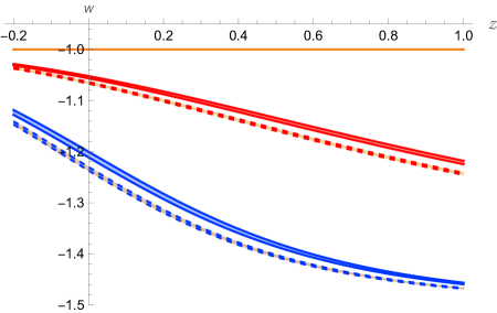
In Fig. 4 we display $w_{f}(z)$ for the three models. Of course $w_{f_{\rm ds}}(z)=-1$. The two other models have negative $w_{f}(z)<-1$. In standard cosmology this is a sign that some unphysical degrees of freedom have been added to the system. However, here one cannot conclude that, since merging with baby universe seems more like having a time dependent cosmological constant, but without the problem that a time dependent cosmological constant will break the invariance of the model under time-reparametrization. Allowing a time dependence of the cosmological “constant”: $\lambda\to\lambda(t)$, changes $w_{f_{\rm ds}}$:

$$w_{f_{\rm ds}}(z)=-1\to w_{\tilde{f}_{\rm ds}}=-1-\frac{1}{3H(t)}\,\frac{\dot{\lambda}(t)}{\lambda(t)}.$$ (46)

Thus, if $\lambda(t)$ is growing with time, assuming the universe is expanding (i.e. $H(t)>0$), it follows that $w_{\tilde{f}_{\rm ds}}(t)<-1$. If we consider the $f_{\rm mod}$ model then $\lambda(t)$ is replaced by $-3g/2p$, and effectively it acts in the same way: for small $t\to 0$ $p(t)\to-\infty$ while for $t\to\infty$ $p(t)\to-(2g)^{1/3}$. In fact using (32) it follows immediately that $w_{f_{\rm mod}}(z)$ goes monotonically from $-3/2$ at $z=\infty$ ($t=0$), to $-1$ for $z=-1$ ($t=\infty$), as also illustrated in Fig. 4.

Figure 4: $w_{f}(z)$ for the three models. The orange curve is $w_{f_{\rm ds}}=-1$, which is true for any value of $H_{0}$. The red curves are for the $f_{\rm gcdt}$-model, dotted curve for $H_{0}^{\rm SC}$ (case A) and full curve for $H_{0}^{\rm CMB}$ (case B). The blue curves are for the $f_{\rm mod}$-model, dotted curve for $H_{0}^{\rm SC}$ (case A) and full curve for $H_{0}^{\rm CMB}$ (case B). For $z\to-1$ ($t\to\infty$) $w_{f}(z)\to-1$.

Finally, in Table 3 we list the various values of $t_{0}$ in the six cases discussed.

	$t_{0}({\rm ds})$	$t_{0}({\rm gcdt})$	$t_{0}({\rm mod})$
case A	13.3 Gyr	13.5   Gyr	13.9  Gyr
case B	13.8  Gyr	14.0  Gyr	14.4  Gyr

Table 3.

In case A $t_{0}({\rm ds})=13.3\;{\rm Gyr}$ and $t_{0}({\rm gcdt})=13.5\;{\rm Gyr}$ seem uncomfortable short and in case B $t_{0}({\rm mod})=14.4\;{\rm Gyr}$ is probably too long. However, had we started out with a $H_{0}$ in between $H_{0}^{\rm SC}$ and $H_{0}^{\rm CMB}$ we can obtain values of both $t_{0}({\rm mod})$ and $t_{0}({\rm gcdt})$ that are comfortable in agreement with the age of the universe as determined from the oldest stars. In particular for the $f_{\rm gcdt}$-model, just looking at the data in Figs. 2 and 3 it is clear that if we tried to determine the best value of $H_{0}$ for the model from the data (including now the observed $H_{0}^{\rm SC}$ as a data point), the optimal value of $H_{0}$ would precisely be between $H_{0}^{\rm SC}$ and $H_{0}^{\rm CMB}$. In Table 4 we have listed values of $H_{0}$ obtained for the three model by minimizing the $\chi^{2}$ for the data shown in Fig. 2, together with the corresponding (minimal) value of the reduced $\chi^{2}$:

	$f_{\rm ds}$-model	$f_{\rm gcdt}$-model	$f_{\rm mod}$-model
$H_{0}$	71.2	72.2	73.9
$\chi_{\rm red}$	2.4	1.2	1.4
$t_{0}$	13.5 Gyr	13.6 Gyr	13.8 Gyr

Table 4.

The $f_{\rm gcdt}$- and $f_{\rm mod}$-models are doing slightly better than the $f_{\rm ds}$-model, but the error bars in Fig. 2 are too large to obtain any precision determination of $H_{0}$ in this way. The same is even more true if one had used the data in Fig. 3 to determine the “best value” of $H_{0}$ for the three models. In Fig. 5 we have shown the equivalent of Fig. 3, using the values of $H_{0}$ from Table 4.

We have here considered the “locally” observed $H(z)$ and $D_{V}(z)$. One could also consider the variable $f_{m}(z)\sigma_{8}(z)$, used for the study of density fluctuation of matter for $z<2$. In [2] this variable is defined precisely and calculated for the three models and compared to measured values. The error bars in the data were too large to distinguish between the models. However, this could change dramatically with new observations to be obtained with the Euclid satellite.

Figure 5: The graphs for $H(z)/(1+z)$ for the three models using the values of $H_{0}$ from Table 4. Orange graph corresponds to $f_{\rm ds}$-model, blue graph to the $f_{\rm mod}$-model and red graph to the $f_{\rm gcdt}$-model.

5 Discussion

Let us start by emphasizing the extreme simplicity of the models considered. It is based on the Hamiltonian

$${\cal H}=N{v}\big{(}-f(p)+\kappa\rho_{\rm m}(v)\big{)},\qquad\rho_{\rm m}(v)v=\rho_{\rm m}(v_{0})v_{0}.$$ (47)

and the corresponding eoms are

$$f(p)=\kappa\rho_{\rm m}(v),\qquad\frac{\dot{v}}{v}=-f^{\prime}(p),\qquad\dot{p}=f(p).$$ (48)

Thus, (for suitable $f$), if the universe starts out with a small spatial volume $v(t)$ for small $t$, $\rho_{\rm m}(v(t))$ is large and the first equation implies that $-p$ is large. The second equation then implies that the expansion is fast, and the last equation that $-p$ increases, i.e. $|p|$ decreases, which again implies that the rate of expansion per unit volume $\dot{v}/v$ decreases. Eventually, if $v(t)$ continues to grow to infinity, $\rho_{\rm m}(v)$ goes to zero. Thus $f(p)$ goes to zero, i.e. $p$ goes to a constant. The middle equation then implies that $v(t)$ approaches an pure exponential expansion. As we have argued, assuming the absorption of baby universes this exponential expansion is very natural if the chance of such an absorption per unit time is proportional to the spatial volume. Therefore, there is no need to introduce a cosmological constant (“negative gravity”) by hand: the gravitational force indeed wants to limit the expansion of the universe, but this is counteracted by the “bombardment” of our Universe by baby universes.

The model we have suggested is of course quite primitive and unrealistic, but taking two limits, one where only universes with infinitesimal spatial volumes are absorbed, the $f_{\rm mod}$ model, and one where universes of any size can be absorbed and where our Universe and the other universes are on equal footing, the $f_{\rm gcdt}$ model, show that the models are reasonable insensitive to the detailed distribution of baby universe sizes. One can therefore hope that they reflect the results one would obtain from more realistic models.

We have presented our model as a “late time” cosmological model and in the present formulation it has nothing to say about the universe for $t<t_{\rm LS}$. Viewed as such a late time cosmological model it is interesting that it favors the local measured value $H_{0}^{\rm SC}$ somewhat compared to the value $H_{0}^{\rm CMB}$. However, in view of the simplicity of the model, we will not press this as an important point. Let us rather discuss if this multi-universe scenario has a chance to answer some of the early-time questions in cosmology.

We have nothing to add about inflation as it is presented in various models. However, the fact that the universe has expanded from, say, a Planckian size to $10^{-5}$m in a very short time, invites the suggestion that this expansion was caused by a collision with a larger universe, i.e. that it was really our Universe which was absorbed in another “parent” universe. Since we have presently no detailed description of the absorption process, it is difficult to judge if such a scenario could take place in a way that would actually solve the problems inflation was designed to solve, but one interesting aspect of such a scenario is that there is no need for an inflaton field.

While a continuous absorption of microscopic baby universes probably can be accommodated in a non-disruptive way in our Universe, it is less clear what happens if the “baby” universe is not small, since we have not suggested an actual mechanism for such absorption. Maybe the least disruptive situation would be one where the absorption happened inside a black hole. The unknown mechanism of absorption could maybe favor such a scenario when the sizes of the baby universes are not infinitesimal. Recall that a Reissner-Nordström black hole actually connects to different universes. We are not seriously suggesting such a black hole scenario, but we mention it to point out that there is room for a lot of interesting considerations. Ultimately, any realistic model should be specific about how the absorption occurs.

The present value of the cosmological constant $\lambda$ in the $\Lambda$CDM model is according to some viewpoints embarrassingly small. According to (19), $\lambda$ being small when expressed in Planck units ($\kappa=1$) also implies that $g$ is small. Historically, before observations pointed to a small $\lambda$ in the $\Lambda$CDM model, many people favored $\lambda=0$ as a result of some underlying mechanism not yet fully understood, e.g. Coleman’s mechanism [21]. We might still need such a mechanism to explain why a $\lambda$ coming from the zero-point fluctuations of quantum fields will not create a large $\lambda$ . However, it might be easier to explain why $\lambda$ is exactly zero than to explain why it is unnaturally small. If $\lambda=0$ can be proven, we could then still have an exponentially expanding universe caused by baby universe absorption.

Like $\lambda$, $g$ appears in our model just as a coupling constant, reflecting in some way the “density” of the baby universes “surrounding” our Universe. By comparing our model to observations $g$ has to be small. However, it is a coupling constant in a larger multiverse theory that we have not yet been able to solve. This leaves the hope that a consistent solution of this larger theory might determine $g$. We have started the program to unveil this theory [3], but it is still work in progress.

Appendix

In this Appendix we list some of the analytical results for the three models defined by $f_{\rm ds}$, $f_{\rm gcdt}$ and $f_{\rm mod}$, respectively. As remarked above we have already analytic parametric representations of all the observables considered, using $\kappa p$ as parameter. Here we will provide the explicit expressions and also provide some of them as analytic functions of time $t$.

The $f_{\rm ds}$-model

$f_{\rm ds}(p)$ is given (38). From (22) we can find $t$ as a function of $p$:

$$t=\int_{-\infty}^{p}\frac{dp^{\prime}}{f_{\rm ds}(p^{\prime})}=-\frac{2}{\sqrt{3\lambda}}\tanh^{-1}\Big{(}\frac{2\sqrt{\lambda}}{\sqrt{3}}\,\frac{1}{p}\Big{)}$$ (49)

$$p=-\frac{2\sqrt{\lambda}}{\sqrt{3}}\coth\Big{(}\frac{\sqrt{3\lambda}}{2}t\Big{)}.$$ (50)

$$f_{\rm ds}(p)=\frac{\lambda}{\sinh^{2}\Big{(}\frac{\sqrt{3\lambda}}{2}\,t\Big{)}},\quad{\rm i.e}\quad v(t)=\frac{\kappa\rho_{\rm m0}v_{0}}{\lambda}\;\sinh^{2}\Big{(}\frac{\sqrt{3\lambda}}{2}\,t\Big{)}$$ (51)

The only non-trivial function is $D_{M}$ defined by eq. (34). The integral can be expressed by hypergeometric functions and one representation is

$$D_{M} = \frac{6}{\sqrt{3\lambda}}\left.\Big{(}\frac{\lambda}{\kappa\rho_{\rm m0}}\Big{)}^{1/3}\sinh^{1/3}\Big{(}\frac{\sqrt{3\lambda}}{2}t^{\prime}\Big{)}\!~{}_{2}F_{1}\Big{[}\frac{1}{6},\frac{1}{2};\frac{7}{6};-\sinh^{2}\Big{(}\frac{\sqrt{3\lambda}}{2}t^{\prime}\Big{)}\Big{]}\right|_{t}^{t_{0}}$$ (52)

$$= \frac{6}{\sqrt{3\lambda}}\,\Big{(}\frac{\lambda}{\kappa\rho_{\rm m0}}\Big{)}^{1/3}\Big{(}\frac{\lambda}{f_{\rm ds}(p^{\prime})}\Big{)}^{1/6}\!\!~{}_{2}F_{1}\left.\Big{[}\frac{1}{6},\frac{1}{2};\frac{7}{6};-\frac{\lambda}{f_{\rm ds}(p^{\prime})}\Big{]}\right|_{p}^{p_{0}}$$ (53)

where

$$\frac{\lambda}{\kappa\rho_{\rm m0}}=\frac{\lambda}{f_{\rm ds}(p_{0})}=\sinh^{2}\Big{(}\frac{\sqrt{3\lambda}}{2}\,t_{0}\Big{)}.$$ (54)

The $f_{\rm gcdt}$-model

$f_{\rm gcdt}(p)$ is given by (39). From (22) we can find $t$ as a function of $p$:

$$t=\int_{-\infty}^{p}\frac{dp^{\prime}}{f_{\rm gcdt}(p^{\prime})}=\frac{4}{3\sqrt{6}\,\alpha}\left(\tanh^{-1}\Big{(}\frac{\sqrt{\frac{2}{3}}(-p+2\alpha)}{\sqrt{(p-\alpha)^{2}+2\alpha^{2}}}\Big{)}-\tanh^{-1}\Big{(}\sqrt{\frac{2}{3}}\Big{)}\right)$$ (55)

Definining $t_{c}$ by

$$\frac{3\sqrt{6}\,\alpha}{4}\;t_{c}=\tanh^{-1}\Big{(}\sqrt{\frac{2}{3}}\Big{)}=\cosh^{-1}\sqrt{3}=\sinh^{-1}\sqrt{2},$$ (56)

we can invert (55) to find:

$$p=-\alpha\,\frac{\sinh\frac{3\sqrt{6}\,\alpha}{4}(t+t_{c})+2\sqrt{2}}{\sinh\frac{3\sqrt{6}\,\alpha}{4}(t+t_{c})-\sqrt{2}}$$ (57)

$$f_{\rm gcdt}(p)=\frac{9\sqrt{3}\,\alpha^{2}}{2}\,\frac{\cosh\frac{3\sqrt{6}\,\alpha}{4}(t+t_{c})}{\big{(}\sinh\frac{3\sqrt{6}\,\alpha}{4}(t+t_{c})-\sqrt{2}\big{)}^{2}}$$ (58)

Again the only non-trivial function is $D_{M}$ defined by eq. (34). In this case the integral in eq. (34) is a generalized hypergeometric functions, a so-called Appell-$F_{1}$ function:

$$D_{M}=\frac{1}{f_{\rm gcdt}(p_{0})^{1/3}}\;\Big{(}\frac{p^{\prime}+\alpha}{6\alpha^{2}}\Big{)}^{1/3}F_{1}\left.\Big{(}\frac{1}{3},\frac{1}{3},\frac{1}{3},\frac{4}{3};x^{+}(p^{\prime}),x^{-}(p^{\prime})\Big{)}\right|_{p}^{p_{0}}$$ (59)

where

$$f_{\rm gcdt}(p_{0})=\kappa\rho_{\rm m0},\qquad x^{\pm}(p)=\frac{2\pm i\sqrt{2}}{3\alpha}\,(p+\alpha).$$ (60)

The $f_{\rm mod}$-model

$f_{\rm mod}(p)$ is given by (40). From (22) we can find $t$ as a function of $p$:

$$t=\int_{-\infty}^{p}\frac{dp^{\prime}}{f_{\rm mod}(p^{\prime})}=\frac{4}{3\sqrt{3}\,a}\Big{(}\arctan\frac{2p-a}{\sqrt{3}\,a}+\frac{1}{2\sqrt{3}}\log\frac{(p-a)^{2}+ap}{(p+a)^{2}}+\frac{\pi}{2}\Big{)}$$ (61)

where

$$a=2^{1/3}\alpha,\qquad t\to 0~{}{\rm for}~{}p\to-\infty,\qquad t\to\infty~{}{\rm for}~{}p\to-a.$$ (62)

Again we can express $D_{M}$, defined by the integrals in eq. (34) , in terms of hypergeometric functions. One representation is:

$$D_{M}=\frac{3}{5}\Big{(}\frac{2}{3}\Big{)}^{2/3}\frac{1}{\alpha^{2}f(p_{0})^{1/3}}\;(p^{\prime})^{5/3}\!~{}_{2}F_{1}\left.\Big{(}\frac{5}{9},\frac{2}{3};\frac{14}{9};-\frac{(p^{\prime})^{3}}{2\alpha^{3}}\Big{)}\right|_{p}^{p_{0}}.$$ (63)

Duality in the $f_{\rm mod}$-model

We end by observing that we have a kind of duality in the $f_{\rm mod}$-model. Define a (modified) Hubble parameter by $h(t)=\dot{v}/v=3\dot{a}/a=3H(t)$, where $H(t)$ is the usual Hubble parameter. We then have the equations:

$$\frac{3}{4}\Big{(}p^{2}+\frac{2\alpha^{3}}{p}\Big{)}=\kappa\rho_{\rm m}(v),\quad h(v)=-\frac{3}{4}\Big{(}2p-\frac{2\alpha^{3}}{p^{2}}\Big{)}.$$ (64)

These equations are invariant under the replacement

$$p\;\longleftrightarrow\;-\frac{\gamma}{\alpha}\frac{\alpha^{3}}{p},\quad\qquad\kappa\rho_{\rm m}\;\longleftrightarrow\;\frac{\alpha}{\gamma}\,h,\qquad\gamma=2^{1/3}.$$ (65)

The mapping $p\to-\gamma\alpha^{2}/p$ has some similarity with a $T$-duality map in string theory.