Automated mapping of virtual environments with visual predictive coding

Abstract

Humans construct internal cognitive maps of their environment directly from sensory inputs without access to a system of explicit coordinates or distance measurements. While machine learning algorithms like SLAM utilize specialized visual inference procedures to identify visual features and construct spatial maps from visual and odometry data, the general nature of cognitive maps in the brain suggests a unified mapping algorithmic strategy that can generalize to auditory, tactile, and linguistic inputs. Here, we demonstrate that predictive coding provides a natural and versatile neural network algorithm for constructing spatial maps using sensory data. We introduce a framework in which an agent navigates a virtual environment while engaging in visual predictive coding using a self-attention-equipped convolutional neural network. While learning a next image prediction task, the agent automatically constructs an internal representation of the environment that quantitatively reflects distances. The internal map enables the agent to pinpoint its location relative to landmarks using only visual information.The predictive coding network generates a vectorized encoding of the environment that supports vector navigation where individual latent space units delineate localized, overlapping neighborhoods in the environment. Broadly, our work introduces predictive coding as a unified algorithmic framework for constructing cognitive maps that can naturally extend to the mapping of auditory, sensorimotor, and linguistic inputs.

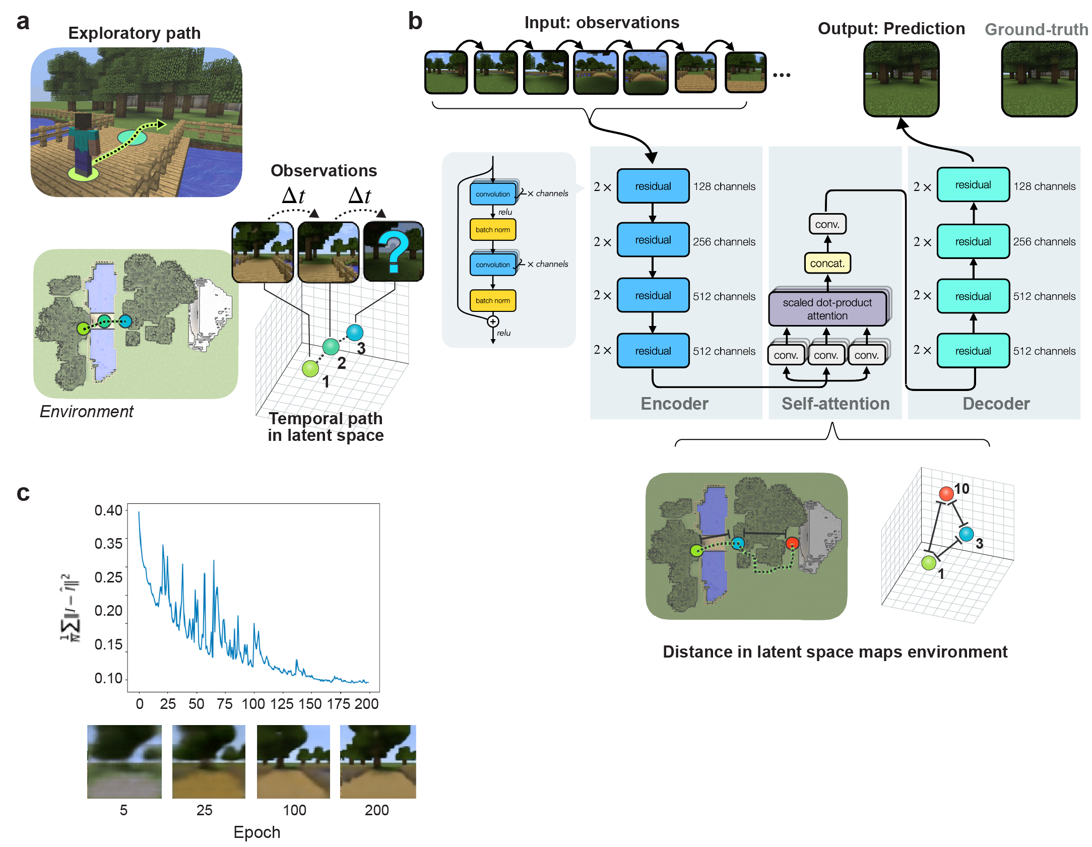
Figure 1: Predictive coding on visual sequences depends on the path in space. a, in predictive coding, a model predicts observations and updates model given the prediction error the latent density using the prediction error. b, a self-attention-based encoder-decoder neural network architecture learns to perform predictive coding. A ResNet-18 convolutional neural network acts as an encoder; self-attention is performed with 8 heads, and a corresponding ResNet-18 convolutional neural network performing decoding to the predicted image.c, the neural network learns to perform predictive coding effectively—with a mean-squared error of 0.094 between the actual and predicted images.

 

Space and time are fundamental physical structures in the natural world, and all organisms have evolved strategies for navigating space to forage, mate, and escape predation[1, 2]. In humans and other mammals the concept of a spatial or cognitive map has been postulated to underlie spatial reasoning tasks[3, 4]. A spatial map is an internal, neural representation of an animal’s environment that can be queried for navigation tasks. Spatial maps, for example, would provide an internal representation of the environment that could be marked with the location of landmarks, food, water, shelter, and could support both navigation and planning. Additionally, neuroscientists have realized that spatial maps generalize to other sensory modes and to higher order concepts to provide potentially similar representations of somatosensory data as well as of more abstract information including language[5]. The neural algorithms underlying spatial mapping might also support higher order reasoning in humans where reasoning could be considered to be a form of navigation and planning within a space of concepts, facts, and ideas. In fact, empirical evidence suggest that the brain uses common cognitive mapping strategies for spatial and non-spatial sensory information so that common mapping algorithms might exist that can map and navigate over not only visual but also semantic information and logical rules inferred from experience[6].

Since the notion of a spatial or cognitive map emerged, the question of how environments are represented within the brain and how the maps can be learned from experience has been a central question in neuroscience[7]. O’ Keefe[7] shows that a subset of CA1 neurons—termed place cells—in the hippocampus show an increased firing rate at particular locations—termed place fields. Place fields can arise and persist without any external stimuli, suggesting that self-movement is an underlying mechanism. The identification of place fields within the hippocampus provided a potential neural substrate for spatial maps. Place cells are neurons that are active when an animal transits through a specific location in an environment. Hafting et al.[8] provides insight into this mechanism with the discovery of neurons in the MEC—termed grid cells—that fire in regular spatial intervals. Grid cells are insensitive to environmental changes, which suggests that grid cells track an organism’s displacement in the environment. Anatomical studies show that grid cells have many connections to place cells[9]. Neuroscientists speculate that place cells integrate grid cell output signals to produce place fields, which supports the theory that grid and place cells develop a map of the environment. In addition, experimental evidence suggests the faculty for spatial mapping underlies mapping of non-spatial sensory variables [10] as well as abstract concepts [11], semantic information [12, 13, 14], and memories [15].

Yet, with the identification of the potential substrate for the representation of space, the question of how a spatial map can be learned from sensory data has remained. In other words, the neural algorithms that enable the construction of spatial and other cognitive maps remain poorly understood. Empirical work in machine learning has demonstrated that deep neural networks can solve spatial navigation tasks as well as perform path prediction and grid cell formation[16, 17]. Cueva & Wei[16] and Banino et al.[17] demonstrate that neural networks can learn to perform path prediction and that networks generate firing patterns that resemble the firing patterns of grid cells in the entorhinal cortex. However, these studies allow an agent to access environmental coordinates explicitly [16] or initialize a model with place cells that represent specific locations in an arena[17]. Further, machine learning studies have focused on demonstrating that a neural network can learn to navigate through training, but these networks remain black boxes and do not reveal the algorithms or computational principles enabling spatial mapping[18, 17, 19]. The algorithms that can enable a system to construct a spatial map directly from sensory data without access to an explicit or implicit coordinate system remain undefined.

Mathematically, mapping questions are related to the idea of embeddings in data analysis and machine learning. Low dimensional embeddings like IsoMap[20] and principal components analysis (PCA) provide a representation of data that organizes data points within a manifold that can be described by a metric organization. The embeddings place data points in proximity to one another based on a notion of relatedness in sensory data. For example, PCA and related non-linear methods can map images with similar structure into proximity within a latent represent. However, proximity is based upon image similarity and not spatial proximity. In machine learning and autonmous navigation, a variety of algorithms have been developed to perform mapping tasks including SLAM and monoclular SLAM algorithms [21, 22, 23, 24] as well as neural network implementations [25, 26, 27]. Yet, SLAM algorithims contain many specific inference strategies like visual feature and object detection that are specifically engineered for map building, way finding, and pose estimation based on visual information. Further, many algorithms make use of distance measurements that contain coordinates implicitly or allow the agent to access global coordinates provided by GPS for refinement. In all cases algorithms must solve the problem of integrating information from local measurements into a global reconstruction of the environment. A unified theoretical and mathematical framework for understanding the mapping of spaces based on sensory information remains incomplete.

Predictive coding has been proposed as a unifying theory of neural function where the fundamental goal of a neural system is to predictive future observations given past data[28, 29, 30]. Classically, predictive coding strategies processes information through a feedback system, in which a learned, internal model predicts sensory observations [31, 32]. When there is a mismatch between predictions and sensory data, an error signal is used to update the predictions and refine the model, leading to a more accurate understanding of the environment. Yet, predictive coding typically acts on time-series data while neglecting space. Predictive coding, instead, proposes an efficient coding system for the sensory observations. As a framework for an efficient coding system, predictive coding has been applied to understand the visual cortex[33, 34], complexity[35], and statistical mechanics[36].

Historically, Poincare motivated the possibility of mapping through a predictive coding strategy where an agent assembles a global representation of an environment by gluing together information gathered through local exploration [37, 38]. In such a strategy an agent could potentially learn the structure of environment by learning how movement within the environment generates group theoretic transformations of visual observations. Poincare imagined an agent that can do such assembly through algebraic operations, for example, by piecing together gathered through exploratory loops that transit and intersect through common locations. The exploratory paths together contain information that could in principle enable the assembly of a spatial map for both flat and curved manifolds. Further, the concept of paths and loops within a space containing information about the underlying topology and geometry of a space is formalized in concepts including homotopy, and holonomy.

Here, we demonstrate that a neural network trained on a predictive coding task can construct an implicit spatial map of environment by assembling information from local paths into a global representation of a physical space within the network’s latent space. The strategy can be implemented by a feed-forward network architecture and embeds images collected by an agent, exploring an environment such that the distances between images within the embedding reflects their relative spatial position, not object-level similarity between images. During exploratory training, the network implicitly assembles information from local paths into a global representation of space as it performs a next image inference problem. Our results depend in an essential way on the prediction task, networks trained as autoencoders can construct representations of space, but these representations are not faithful to spatial geometry when two regions of an agent’s environment have common visual landmarks. Our work extends the application of predictive coding tasks to the construction of geometric maps from sensory data streams without explicit access to distance measurements or other spatial cues. Our results suggest that prediction tasks provide an integrated mathematical framework in which spatial maps can be assembled from sensory data demonstrating that mapping problems can be solved naturally without a great deal of mathematical machinery. Our work might also shed light on the power of causal language modeling or next word prediction tasks in machine learning. Fundamentally, we connect predictive coding and mapping tasks and shows that provides a computational and mathematical strategy for integrating information from local measurements into a global self-consistent environmental model.

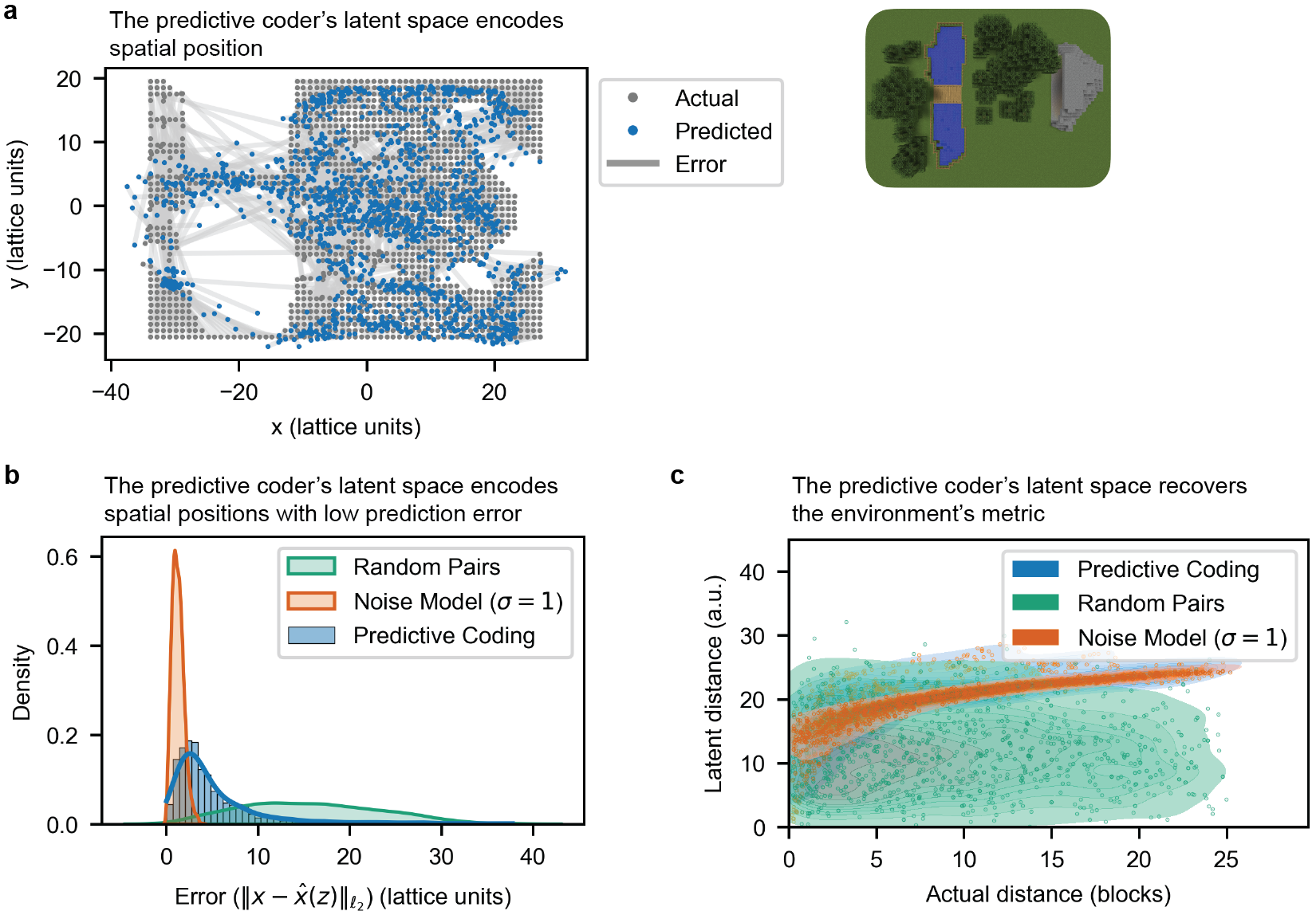
Figure 2: A neural network that performs predictive coding recovers the environment’s spatial position and distance. a-b, The latent space encodes spatial position. b, a neural network predicts the spatial location from the predictive coding’s latent space. b, predictive coding’s latent space encodes spatial position. The histogram of prediction errors of positions from the predictive coder’s latent space. The additive noise model and the random shuffle model provides baselines for the minimum and maximum errors, respectively. c, predictive coding’s latent distances recover the environment’s spatial metric. Sequential visual images are mapped to the neural network’s latent space, and the latent space distances ($\ell_{2}$) are plotted with physical distances onto a joint density plot.

 

1 Mathematical formulation of spatial mapping as predictive coding

We consider an agent exploring an environment, $\Omega\subset\mathbb{R}^{2}$, while acquiring visual information in the form of pixel valued images $I(x)\in\mathbb{R}^{m\times n}$. We take the agent’s environment to be a bounded subset or $\mathbb{R}^{2}$ that could contain obstructions and holes. At any given time, $t$, the agent’s state can be characterized by a position $x(t)$ and orientation $\theta(t)$ where $x(t)$ and $\theta(t)$ are coordinates within a global coordinate system unknown to the agent. While both $x$ and $\theta$ can be accommodated within our statistical inference framework, we motivate, first, consider an agent that adopts a constant orientation while moving along a series of positions $x(t)$.

The agent’s environment comes equipped with a visual scene and the agent makes observations by acquiring image vectors $I_{x_{k}}$ as it moves along a sequence of points $x_{k}$. At every position x , the agent acquires an image, $I(x)\in\mathbb{R}^{m\times n}$ by sampling from an image the conditional probability distribution $P(I|x)$ which encodes the probability of observing a specific image vector $I$ when the agent is positioned at $x$ with ore. Mathematically, we can view $P(I|x)$ as a function on a vector bundle with base space and total space $\Omega\times I$. For simplicity, we consider an agent that moves through an environment by executing a series of local steps $x(t+dt)=x(t)+v_{k}\ dt$ where $v_{k}$ is a velocity and $dt$ is a time scale associated with movement and image acquisition, so that we take the motion of the agent to be generated by a Markov process with transition probabilities $P(x_{i+1}|x_{i})$. The distribution $P(I|x)$ has a deterministic and stochastic component where the deterministic component is set by landmark’s in the environment while stochastic effects could emerge due to changes in lighting and other background dynamics.

In the predictive coding problem, the agent moves along a series of points $x_{0},x_{1},\dots,x_{k}$ while acquiring images $I_{0},I_{1},\dots I_{k}$. Note that the agent has access to the image observations $I_{i}$ but not the coordinates $x_{i}$. Given the set $\{I_{0}\dots I_{k}\}$ the agent aims to predict $I_{k+1}$. Mathematically, statistical inference of the image prediction problem can proceeds by (a) inferring the posterior probability distribution $P(I_{k+1}|I_{0},I_{1}....I_{k})$ from observations and, then (b) given a specific sequence $\{I_{0}\dots I_{k}\}$, the agent can make predictions by finding the image $I_{k+1}$ that maximizes the posterior probability distribution $P(I_{k+1}|I_{0},I_{1}....I_{k})$.

The key challenge in the problem is the functional representation and parameterization of $P(I_{k+1}|I_{0},I_{1}....I_{k})$ from observations. We will solve both problems, ultimately, with an encoder-decoder neural network. However, the architecture of that network can be motivated by, first, analyzing the structure of the statistical inference problem and posterior probability distribution $P(I_{k+1}|I_{0},I_{1}....I_{k})$ .

$$P(I_{k+1}|I_{0},I_{1}....I_{k})=\frac{P(I_{0},I_{1}....I_{k},I_{k+1})}{P(I_{0},I_{1}....I_{k})}$$

Now, we can consider $P(I_{0},I_{1}\dots I_{k},I_{k+1})$ to be an implicit function on an implicit set of spatial coordinates $x_{i}$ where $x_{i}$ are arbitrary and are not accessible to the agent.

 

$$P(I_{k+1}|I_{0},I_{1}\ldots.I_{k}) =\intslop\ilimits@\mathbf{dx}\ P(x_{0}...x_{k})\frac{P(I_{0},I_{1}\cdots I_{k}|x_{0}...x_{k})}{P(I_{0},I_{1}....I_{k})}P(x_{k+1}|x_{k})P(I_{k+1}|x_{k+1})$$

$$=\intslop\ilimits@\ \mathbf{dx}\ \underbrace{P(x_{0}...x_{k}|I_{0},I_{1}\cdots I_{k})}_{\text{encoding }(1)}\underbrace{P(x_{k+1}|x_{k})}_{\text{spatial transition probability }(2)}\underbrace{P(I_{k+1}|x_{k+1})}_{\text{decoding }(3)}$$ (1)

 

where in general the integration is over all possible paths $\{x_{0}\dots x_{k}\}$ in the domain so that $\mathbf{dx}=dx_{i}\dots dx_{k}$. Equation 1 can be interpreted as a path integral over the domain where term 1 assigns a probability to every potential path $\{x_{0}\dots x_{k}\}\in\Omega$ based upon the conditional likelihood of the path given the observed sequences of images $\{I_{0}\dots I_{k}\}$ and the transition functions $P(x_{i+1}|x_{i})$. The second term computes the probability that an agent at at terminal position $x_{k}$ moves to the position $x_{k+1}$, and the third term encodes the probability that images $I_{k+1}$ is observed given that the agent is at position $x_{k+1}$. The path integral assigns a probability to every possible path in the domain and then computes the probability that the agent will observe a next image $I_{k}$ along each path given the agents internal model of the environment $P(I_{k+1}|x_{k+1})$.

Equation 1 solves the next image prediction problem in three steps. First (1), estimating the probability that an agent has traversed a particular sequence of points given the observed image observations; second (2), estimating the next position of the agent $x_{k+1}$ for each potential path; and third (3), computing the probability of generating image $I_{k+1}$ given that inferred final location $x_{k+1}$. Importantly, the algorithm implied by these equations would construct an internal but implicit representation of the environment as an internal coordinate system $\mathbf{x}$ that is integrated out during the inference computation. In this way, the internal coordinate system could be an arbitrary $x^{\prime}=Px$ where $P\in\text{SO}(2)$ is transformation by rotation of basis elements. The coordinate system is in this way arbitrary, but is used in the computation as an internal, inferred representation of the agent’s environment that is used to estimate future image observation probabilities.

As is common in statistical inference, the implementation challenge is the parameterization and estimation of the encoding map $P(x_{0}\dots x_{k}|I_{0}\dots I_{k})$, transition map $P(x_{k+1}|x_{k})$, and decoding map $P(I_{k+1}|x_{k+1})$ given data. Yet, critically, the path-integral equation for $P(I_{k+1}|I_{0}\dots I_{k})$ is a chain of products that can naturally be represented in a neural network architecture. The first term acts as an ‘encoder’ network that computes encoding the probability that the agent has traversed a path $x_{0}...x_{k}$ given an observed image sequence $I_{0},\ldots,I_{k}$ that is fed into the network (Figure 1(b)). The network can, then, estimate the next position of the agent $x_{k+1}$ given an inferred location $x_{k}$, and apply a decoding network to compute $P(I_{k+1}|x_{k+1})$ while outputting $I_{k+1}$. The network would be trained through visual experience, and thus, must learn an internal coordinate system and representation $\mathbf{x}$ that provides a representation of the environment and also links images $I_{j}$ to inferred locations $x_{j}$.

In this way, the next image prediction problem can be solved by an agent that constructs an implicit representation of the spatial environment. Our central insight is that the internal representation of the environment, dependent only on sensory data, can then be used directly as an internal cognitive map.

A neural network can accurately perform predictive coding

Motivated by the implicit representation of space contained in the predictive coding inference problem, we developed a computational implementation of a predictive coding agent, and studied the representation of space learned by that agent as it explored a virtual environment, generated using the Malmo environment for Minecraft[39]. We developed an environment with a series of distinct virtual regions including a forest, a stream, and a cave. Each region has a distinct set of visual scenes.

To demonstrate that a neural network—without the environment’s coordinates—can map an environment by performing predictive coding directly on visual input, we construct a neural network that performs predictive coding. We first create an environment with the Malmo environment in Minecraft[39]. The physical environment measures $40\times 65$ lattice units and encapsulates three aspects of visual scenes: first, a cave provides a global visual landmark; second, a forest provides degeneracy between visual scenes; and third, a river with a bridge constraints an agent’s traversal in the environment (Figure 1(a)). An agent traverses paths determined by $A^{*}$ search between randomly sampled positions and receives visual images along every path.

To perform predictive coding, we construct an encoder-decoder convolutional neural network with a ResNet-18 architecture[40] for the encoder and a corresponding ResNet-18 architecture with transposed convolutions in the decoder (Figure 1(b)). The encoder-decoder architecture uses the U-Net architecture[41] to pass the encoded latent units into the decoder. Multi-headed attention[42] processes the sequence of encoded latent units to encode the history of past visual observations. The multi-headed attention has $h=8$ heads. For the encoded latent units with dimension $D=C\times H\times W$, the dimension $d$ of a single head is $d=C\times H\times W/h$.

The predictive coder approximates predictive coding by minimizing the mean-squared error between the actual observation and its predicted observation. The predictive coder trains on $82,630$ samples for $200$ epochs with gradient descent optimization with Nesterov momentum[43], a weight decay of $5\times 10^{-6}$, and a learning rate of $10^{-1}$ adjusted by OneCycle learning rate scheduling[44]. The optimized predictive coder has to a mean-squared error between the predicted and actual images of $0.094$ and a good visual fidelity (Figure 1(c)).

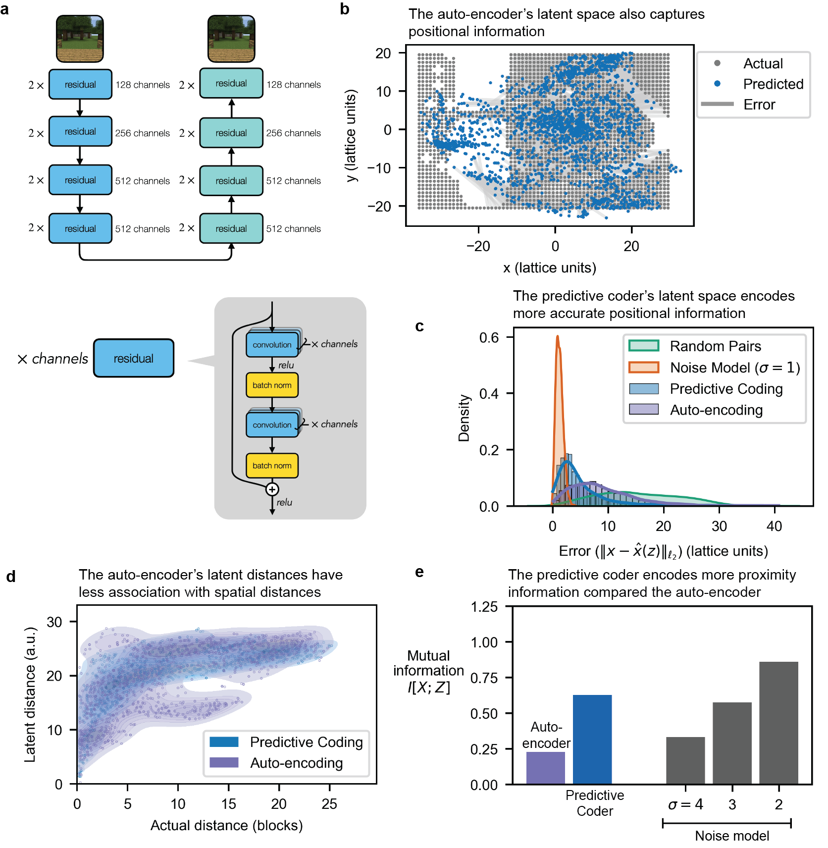
Figure 3: Sequential dependencies—as opposed to visual similarity—encodes the majority of the environment’s position and distance. a, an autoencoding neural network compresses visual images into a low-dimensional latent vector and reconstructs the image from the latent space. Auto-encoder trains on visual images from the environment without any sequential order. b-c, auto-encoding encodes lower resolution in positional information. b, a neural network predicts the spatial location from the auto-encoding’s latent space. c, auto-encoding captures less positional information compared to predictive coding. The histogram shows the prediction errors of positions from the latent space of both the auto-encoder and the predictive coder. d, latent distances, however, show a weaker relationship with physical distances, as the joint histogram between physical and latent distances is less concentrated. e, predictive coding’s latent units communicate more fine-grained spatial distances whereas auto-encoding communicates broad spatial regions. Joint density plots show the association between latent distances and physical distances for both predictive coding and auto-encoding. Predictive coding’s latent distances increases with spatial distances, with a higher concentration compared to auto-encoding.

2 Predictive coding network constructs implicit spatial map

We show that the predictive coder creates an implicit spatial map by demonstrating it recovers the environment’s spatial position and distance. We encode the image sequences using the predictive coder’s encoder to analyze the encoded sequence as the predictive coder’s latent units. To measure the positional information in the predictive coder, we train a neural network to predict the agent’s position from the predictive coder’s latent units (Figure 1(a)). The neural network’s prediction error

$$E(x,\hat{x})=\left\lVert\hat{x}-x\right\rVert_{\ell_{2}}$$

indirectly measures the predictive coder’s positional information. To provide comparative baselines, we construct two different position prediction models to lower bound and upper bound the prediction error. To lower bound the prediction error, we construct a model that gives the agent’s actual position with small additive Gaussian noise

$$\hat{x}=x+\epsilon,\epsilon\sim\mathcal{N}(0,\sigma)$$

To upper bound the prediction error, we construct a model that shuffles the agent’s actual position without replacement. To compare predictive coder to the baselines, we compare the prediction error histograms (Figure 2(b)).

The predictive coder encodes the environment’s spatial position to a low prediction error (Figure 2.d). The predictive coder has a mean error of $5.04$ lattice units and $>80\%$ of samples have an error $<7.3$ lattice units. The additive Gaussian model with $\sigma=4$ has a mean error of $4.98$ lattice units and $>80\%$ of samples with a error $<7.12$ lattice units. The shuffle model, on the other hand, has a mean error of $15.87$ lattice units and $>80\%$ of samples have an error $<22.24$ lattice units.

We show the predictive coder’s latent space recovers the local distances between environment’s physical positions. For every path that the agent traverses, we calculate the local pairwise distances in physical space and in the predictive coder’s latent space with a neighborhood of 100 time points. To determine whether latent space distances correspond to physical distances, we calculate the joint density between latent space distances and physical distances (Figure 2(c)). We model the latent distances by fitting the physical distances with additive Gaussian noise to a logarithmic function

$$d(z,z^{\prime})=\alpha\log(\left\lVert x-x^{\prime}+\epsilon\right\rVert)+\beta,\epsilon\sim\mathcal{N}(0,\sigma).$$

In addition, as a null distribution, we shuffle the physical positions and calculate the latent distances on this shuffled set. The modeled distribution is concentrated with the predictive coder’s distribution with a Kullbeck-Lieber divergence $(\mathbb{D}_{\text{KL}}(p_{\text{PC}}\Vert p_{\text{model}}))$ of $0.429$ bits. The null distribution shows a low overlap with the predictive coder’s distribution with a $\mathbb{D}_{\text{KL}}(p_{\text{PC}}\Vert p_{\text{null}})$ of $2.441$ bits.

3 Temporal dependencies—rather than visual similarity—encode the majority of spatial position and proximity

In the previous section, we show a neural network that performs predictive coding encodes its physical position and local physical distances in its latent space. Principal components analysis and IsoMap[20] can collocate images by visual similarity. Further, autoencoder networks are commonly used to embed images within a latent space where images are embedded by image proximity. We note that such representations encode image proximity but not physical proximity and would not be sufficient for mapping. A neural network that performs predictive coding could be encoding physical position and local distance information by visual similarity—as images from nearby positions are much more similar compared to images at distant positions. Temporal dependencies may then not communicate any spatial information. We refute this explanation and demonstrate that, while visual similarity communicates spatial information, temporal dependencies encode the majority of the environment’s spatial information.

To show the temporal dependencies encode the majority of spatial information, we introduce an auto-encoder with the same architecture as the predictive coder. The auto-encoder is an encoder-decoder convolutional neural network that encodes a single observation—rather than a sequence of past observations—and decodes the same observations. Instead of predicting future observations, the auto-encoder compresses an observation into a low-dimensional latent space. As the auto-encoder only operates on a single image—rather than a sequence, the auto-encoder can only capture features on the single image, which we define as visual similarity. The predictive coder captures features across the sequence of images, in addition to a single image, which includes temporal dependencies between images and visual similarity of a single image.

As with the predictive coder, the auto-encoder (Figure 3(a)) trains to minimize the mean-squared error between the actual image and the predicted image on $82,630$ samples for $200$ epochs with gradient descent optimization with Nesterov momentum, a weight decay of $5\times 10^{-6}$, and a learning rate of $10^{-1}$ adjusted by the OneCycle learning rate scheduler. The auto-encoder has mean-squared error of $0.039$ and a high visual fidelity.

We first demonstrate that the predictive coder—compared to the auto-encoder—encodes more positional information in its latent space. As with the predictive coder, we train a neural network to predict the agent’s position from the auto-encoder’s latent units (Figure 3(b)). The neural network’s prediction error indirectly measures the auto-encoder positional information. The auto-encoder has greater than $80\%$ of its points have a prediction error of less than $13.1$ lattice units, as compared to the predictive coder that has $>80\%$ of its samples have a prediction error of $7.3$ lattice units (Figure 3(c)).

We also show that the predictive coder recovers the environment’s spatial distances with finer detail compared to the auto-encoder. As with the predictive coder, we calculate the local pairwise distances in physical space and in the auto-encoder’s latent space, and we generate the joint density between the physical and latent distances (Figure 3d). Compared to the predictive coder’s joint density, the auto-encoder’s latent distances increase with the agent’s physical distance. The auto-encoder’s joint density shows a larger dispersion compared to predictive coder’s joint density, indicating that the auto-encoder encodes spatial distances with higher uncertainty.

We can quantitatively measure the dispersion in the auto-encoder’s joint density by calculating mutual information of the joint density (Figure 3(e))

$$I[X;Z]=\mathbb{E}_{p(X,Z)}\left[\log\frac{p(X,Z)}{p(X)p(Z)}\right].$$

The auto-encoder has a mutual information of $0.227$ bits while the predictive coder has a mutual information of $0.627$ bits. As a comparison, positions with additive Gaussian noise having a standard deviation $\sigma$ of $2$ lattice units has a mutual information of $0.911$ bits. The predictive coder encodes $0.400$ additional bits of distance information to the auto-encoder. The predictive coder’s additional distance information of $0.4$ bits exceeds the auto-encoder’s distance information of $0.227$ bits, which indicates the temporal dependencies encoded by the predictive coder capture more spatial information compared to visual similarity.

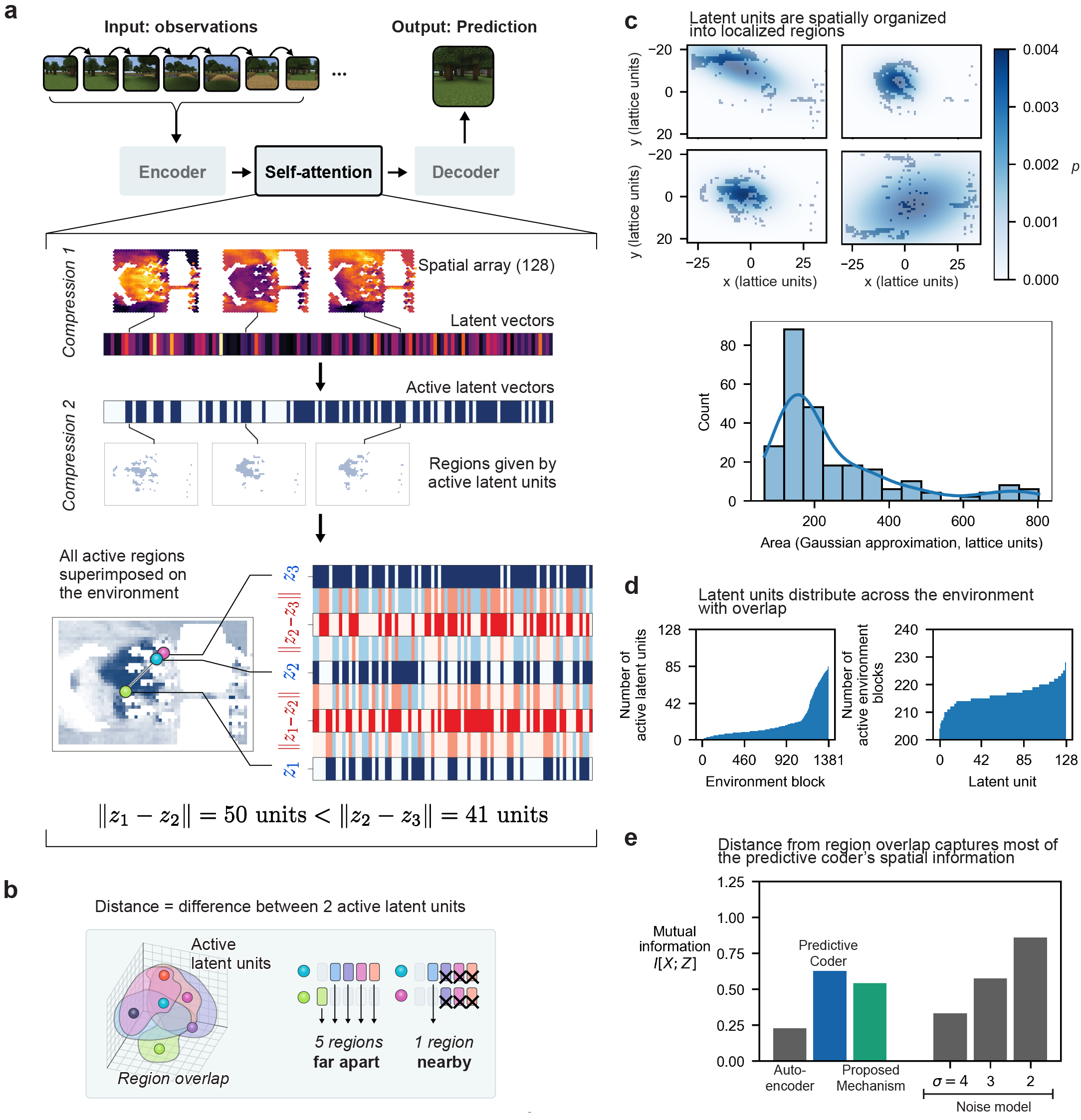
Figure 4: The predictive coding neural network encodes distances using spatially localized latent units. a, when encoding past images for predictive coding, the self-attention module generates latent vectors. Each continuous unit in these latent vectors activate in concentrated, localized regions in physical space. These continuous units can be thresholded to generate a binary vector determining whether each unit is active. Each latent unit covers a unique region, and each physical location gives a unique combination of these overlapping regions. As an agent moves away from its original location, the combination of overlapping regions gradually deviates from its original combinations. These deviation as measured by Hamming distance correlates with physical distance. b, distance is given by the difference in the latent units’ overlapping regions. Two nearby locations have small deviations in overlap (right) while two distant location have large deviations (middle). c, latent units are spatially organized into localized regions. The active latent units are approximated by a two-dimensional Gaussian distribution to measure the latent unit’s localization (top). The latent units’ Gaussian approximations are highly localized with a mean area of $254.6$ for densities $p\geq 0.0005$. d, latent units distributed across the environment. The number of latent units was calculated as each lattice block in the environment (left), and the number of lattice blocks were calculated for each active unit (right). The latent units provide a unique combination for $87.6\%$ of the environment, and their aggregate covers the entire environment. e, distance from the region overlap captures most of the predictive coder’s spatial information. We calculate the distance for every pair of active latent vectors and their respective physical Euclidean distances as a joint distribution. The proposed mechanism captures a majority of the predictive coder’s spatial information—as the proposed mechanism’s mutual information (0.542 bits) compares to the predictive coder’s mutual information (0.627 bits)

4 Predictive coding encodes distances using spatially localized latent units

In the previous section, we demonstrate that the neural network that performs predictive coding uses temporal dependencies to capture the majority of the environment’s spatial information. While temporal dependencies recover significant spatial information about the environment, it is unclear how the neural network encodes temporal information into spatial information. Here we demonstrate that each unit in the neural network’s latent space activates at distinct, localized regions—called place fields—in the environment’s physical space (Figure 4(a)). These place fields overlap with each other and their aggregate covers the entire physical space. At each physical location, there exists a unique combination of overlapping regions form by the latent units. This combination of overlapping regions provide both recover the agent’s current physical position. Moreover, given two physical location, these exist two different combinations of overlapping regions. The differences in these two combinations, that is the Hamming distance, provide the distance between two physical locations (Figure 4(b)). By comparing the combinations of overlapping regions at different positions, the neural network can perform vector navigation given its place fields.

To support this proposed mechanism, we first demonstrate the neural network generates place fields. In other words, units from neural network’s latent space produce localized regions in physical space. To determine whether a latent unit is active, we threshold the continuous value with its 90th-percentile value. To measure a latent unit’s localization in physical space, we fit each latent units distribution with respect to physical space to a two-dimensional Gaussian distribution (Figure 4(c), top)

$$p=\frac{1}{2\pi|\Sigma|}\exp\left[-\frac{1}{2}(x-\mu){}^{-1}(x-\mu)\right]$$

We measure the area of the ellipsoid given by the Gaussian approximation where $p\geq 0.0005$ (Figure 4(c), bottom). The area of the latent unit approximation measures how localized a unit is compared to the environment’s area, which measures $40\times 65=2,600$ lattice units. The latent unit approximations have a mean area of $254.6$ lattice units and a $80\%$ of areas are $<352.6$ lattice units, which cover $9.79\%$ and $13.6\%$ of the environment, respectively.

We demonstrate, in addition, that the units in the neural network’s latent space provide a unique combinations at each position, and the aggregate of latent units covers the environment’s entire physical space. At each lattice block in the environment, we calculate the number of active latent units (Figure 4(d), left). The number of active latent units is different in $87.6\%$ of the lattice blocks. Every lattice block has at least one active latent unit, which indicates the aggregate of the latent units cover the environment’s physical space.

Lastly, we demonstrate that the neural network performs measures physical distances and performs vector navigation by comparing the combinations of overlapping regions in its latent space. We first determine the active latent units by thresholding each continuous value by its 90th-percentile value. At each position, we have a 128-dimensional binary vector that gives the overlap of 128 latent units. At every two positions, we calculate the Hamming distance between each binary latent vector as well as the physical Euclidean distance (Figure 4(a), bottom). Similar to the Sections 2 and 3, we compute the joint densities of the binary vectors’ Hamming distances and the physical positions’ Euclidean distances. We then calculate their mutual information to measure how much spatial information the Hamming distance captures. The proposed mechanism for the neural network’s distance measurement—the binary vector’s Hammi distance—gives a mutual information of $0.542$ bits, compared to the predictive coder’s mutual information of $0.627$ bits and the auto-encoder’s mutual information of $0.227$ bits (Figure 4(e)). Compared to the auto-encoder, the proposed mechanism captures a majority amount of the predictive coder’s spatial information.

5 Discussion

Mapping is a general mechanism that generates an internal representation for organizing sensory information. Spatial maps facilitate navigation and planning within an environment. Mapping, furthermore, is a ubiquitous neural function that extends to neural representations beyond visual-spatial mapping. The primary sensory cortex (S1), for example, maps tactile events topographically within the brain region: physical touches that occur in close proximity are mapped in close proximity for both the neural representations and the anatomical brain regions[45]. Similarly, the cortex maps natural speech by tiling regions by different words and their relationships, which show that topographic maps in the brain extend to higher order cognition. The similar representation of non-spatial and spatial maps in the brain suggest a common mechanism for charting cognitive maps[46]. However, it is unclear how a single mechanism can generate both spatial and non-spatial maps.

Here, we show that predicting sensory data from past sensory experiences—called predictive coding—provides a basic, general mechanism for charting spatial maps. We demonstrate a neural network that performs predictive coding can construct an implicit spatial map of an environment by assembling information from local paths into a global frame within the neural network’s latent space. The implicit spatial map depends specifically on the sequential task of predicting future visual images, for neural networks trained as auto-encoders do not reconstruct a faithful geometric representation in the presence of physically distant yet visually similar landmarks.

Moreover, we study the predictive coding neural network’s representation in latent space. Each unit in the network’s latent space activates at distinct, localized regions—called place fields—with respect to physical space. At each physical location, there exists a unique combinations of overlapping place fields. At two locations, the differences in the combinations of overlapping place fields provides the distance between the two physical locations. The existence of place fields in both the neural network and the hippocampus[7] suggest that predictive coding—by predicting future sensory input—is a universal mechanism for mapping. In addition, vector navigation emerges naturally from predictive coding by computing distances from overlapping place field units. Predictive coding may provide a model for understanding how place cells emerge, change, and function.

Predictive coding can be performed over any sensory modality that has some temporal sequence. As natural speech forms a cognitive map, predictive coding may underlie the geometry of human language. Intriguingly, large language models train on causal word prediction, a form of predictive coding, build internal maps that support generalized reasoning, answer questions, and mimic other forms of higher order reasoning[47]. Similarities in spatial and non-spatial maps in the brain suggest that large language models organize language into a cognitive map and chart concepts geometrically. These results all suggest that predictive coding might provide a unified theory for building representations of information—connecting disparate theories including place cell formation in the hippocampus, somatosensory maps in the cortex, and human language.

References

- [1] Russell A. Epstein, Eva Zita Patai, Joshua B. Julian and Hugo J. Spiers “The Cognitive Map in Humans: Spatial Navigation and Beyond” In Nature Neuroscience 20.11 Nature Publishing Group, 2017, pp. 1504–1513
- [2] Zitong Jerry Wang and Matt Thomson “Localization of signaling receptors maximizes cellular information acquisition in spatially structured natural environments” In Cell Systems 13.7 Elsevier, 2022, pp. 530–546
- [3] John Anderson “Cognitive Psychology and Its Implications” New York City: Worth Publishers, 2020
- [4] Michael Rescorla “Cognitive maps and the language of thought” In The British Journal for the Philosophy of Science The University of Chicago Press, 2009
- [5] Alexander G. Huth et al. “Natural Speech Reveals the Semantic Maps That Tile Human Cerebral Cortex” In Nature 532.7600 Nature Publishing Group, 2016, pp. 453–458
- [6] Timothy EJ Behrens et al. “What is a cognitive map? Organizing knowledge for flexible behavior” In Neuron 100.2 Elsevier, 2018, pp. 490–509
- [7] John O’Keefe “Place Units in the Hippocampus of the Freely Moving Rat” In Experimental Neurology 51.1, 1976, pp. 78–109
- [8] Torkel Hafting et al. “Microstructure of a Spatial Map in the Entorhinal Cortex” In Nature 436.7052 Nature Publishing Group, 2005, pp. 801–806
- [9] D.. Amaral, N. Ishizuka and B. Claiborne “Neurons, Numbers and the Hippocampal Network” In Progress in Brain Research 83, 1990, pp. 1–11
- [10] Dmitriy Aronov, Rhino Nevers and David W. Tank “Mapping of a Non-Spatial Dimension by the Hippocampal–Entorhinal Circuit” In Nature 543.7647 Nature Publishing Group, 2017, pp. 719–722
- [11] Edward H. Nieh et al. “Geometry of Abstract Learned Knowledge in the Hippocampus” In Nature 595.7865 Nature Publishing Group, 2021, pp. 80–84
- [12] Alexandra O. Constantinescu, Jill X. O’Reilly and Timothy E.. Behrens “Organizing Conceptual Knowledge in Humans with a Gridlike Code” In Science 352.6292 American Association for the Advancement of Science, 2016, pp. 1464–1468
- [13] Mona M Garvert, Raymond J Dolan and Timothy EJ Behrens “A Map of Abstract Relational Knowledge in the Human Hippocampal–Entorhinal Cortex” In eLife 6 eLife Sciences Publications, Ltd, 2017, pp. e17086
- [14] Alexander G. Huth et al. “Natural Speech Reveals the Semantic Maps That Tile Human Cerebral Cortex” In Nature 532.7600 Nature Publishing Group, 2016, pp. 453–458
- [15] Suzanne Corkin “Lasting Consequences of Bilateral Medial Temporal Lobectomy: Clinical Course and Experimental Findings in H.M.” In Seminars in Neurology 4.02 © 1984 by Thieme Medical Publishers, Inc., 1984, pp. 249–259
- [16] Christopher J. Cueva and Xue-Xin Wei “Emergence of Grid-like Representations by Training Recurrent Neural Networks to Perform Spatial Localization” In arXiv:1803.07770 [cs, q-bio, stat], 2018 arXiv:1803.07770 [cs, q-bio, stat]
- [17] Andrea Banino et al. “Vector-Based Navigation Using Grid-like Representations in Artificial Agents” In Nature 557.7705 Nature Publishing Group, 2018, pp. 429–433
- [18] David Marr and W Thomas Thach “A theory of cerebellar cortex” In From the Retina to the Neocortex: Selected Papers of David Marr Springer, 1991, pp. 11–50
- [19] Ben Sorscher, Gabriel Mel, Surya Ganguli and Samuel Ocko “A Unified Theory for the Origin of Grid Cells through the Lens of Pattern Formation” In Advances in Neural Information Processing Systems 32 Curran Associates, Inc., 2019, pp. 10003–10013
- [20] Joshua B. Tenenbaum, Vin Silva and John C. Langford “A Global Geometric Framework for Nonlinear Dimensionality Reduction” In Science 290.5500 American Association for the Advancement of Science, 2000, pp. 2319–2323
- [21] Sebastian Thrun and Michael Montemerlo “The Graph SLAM Algorithm with Applications to Large-Scale Mapping of Urban Structures” In The International Journal of Robotics Research 25.5-6, 2006, pp. 403–429
- [22] Raúl Mur-Artal and Juan D. Tardós “Visual-Inertial Monocular SLAM With Map Reuse” In IEEE Robotics and Automation Letters 2.2, 2017
- [23] Anastasios I. Mourikis and Stergios I. Roumeliotis “A Multi-State Constraint Kalman Filter for Vision-aided Inertial Navigation” In Proceedings 2007 IEEE International Conference on Robotics and Automation, 2007, pp. 3565–3572
- [24] Simon Lynen et al. “Get Out of My Lab: Large-scale, Real-Time Visual-Inertial Localization”, 2015
- [25] Saurabh Gupta et al. “Cognitive Mapping and Planning for Visual Navigation” arXiv, 2019 arXiv:1702.03920 [cs]
- [26] Piotr Mirowski et al. “Learning to Navigate in Cities Without a Map” In Advances in Neural Information Processing Systems 31 Curran Associates, Inc., 2018
- [27] Yan Duan et al. “RL2: Fast Reinforcement Learning via Slow Reinforcement Learning”, 2016
- [28] Tai Sing Lee and David Mumford “Hierarchical Bayesian inference in the visual cortex” In JOSA A 20.7 Optica Publishing Group, 2003, pp. 1434–1448
- [29] David Mumford “Pattern theory: a unifying perspective” In First European Congress of Mathematics: Paris, July 6-10, 1992 Volume I Invited Lectures (Part 1), 1994, pp. 187–224 Springer
- [30] Rajesh P.. Rao and Dana H. Ballard “Predictive Coding in the Visual Cortex: A Functional Interpretation of Some Extra-Classical Receptive-Field Effects” In Nature Neuroscience 2.1 Nature Publishing Group, 1999, pp. 79–87
- [31] D Mumford “On the Computational Architecture of the Neocortex”
- [32] Alan Yuille and Daniel Kersten “Vision as Bayesian Inference: Analysis by Synthesis?” In Trends in Cognitive Sciences 10.7, Special Issue: Probabilistic Models of Cognition, 2006, pp. 301–308
- [33] David J. Heeger “Theory of Cortical Function” In Proceedings of the National Academy of Sciences 114.8 Proceedings of the National Academy of Sciences, 2017, pp. 1773–1782
- [34] Stephanie E. Palmer, Olivier Marre, Michael J. Berry and William Bialek “Predictive Information in a Sensory Population” In Proceedings of the National Academy of Sciences 112.22, 2015, pp. 6908–6913
- [35] William Bialek, Ilya Nemenman and Naftali Tishby “Predictability, Complexity, and Learning” In Neural Computation 13.11, 2001, pp. 2409–2463
- [36] Susanne Still, David A. Sivak, Anthony J. Bell and Gavin E. Crooks “Thermodynamics of Prediction” In Physical Review Letters 109.12, 2012, pp. 120604
- [37] Henri Poincaré “The Foundations of Science: Science and Hypothesis, the Value of Science, Science and Method”, Cambridge Library Collection Cambridge: Cambridge University Press, 2015
- [38] John O’Keefe and Lynn Nadel “The Hippocampus as a Cognitive Map” Oxford : New York: Clarendon Press ; Oxford University Press, 1978
- [39] Matthew Johnson, Katja Hofmann, Tim Hutton and David Bignell “The Malmo Platform for Artificial Intelligence Experimentation” In International Joint Conference on Artificial Intelligence, 2016
- [40] Kaiming He, Xiangyu Zhang, Shaoqing Ren and Jian Sun “Deep Residual Learning for Image Recognition” In arXiv:1512.03385 [cs], 2015 arXiv:1512.03385 [cs]
- [41] Olaf Ronneberger, Philipp Fischer and Thomas Brox “U-Net: Convolutional Networks for Biomedical Image Segmentation” arXiv, 2015 arXiv:1505.04597 [cs]
- [42] Ashish Vaswani et al. “Attention Is All You Need” arXiv, 2023 arXiv:1706.03762 [cs]
- [43] Ilya Sutskever, James Martens, George Dahl and Geoffrey Hinton “On the Importance of Initialization and Momentum in Deep Learning”
- [44] Leslie N. Smith and Nicholay Topin “Super-Convergence: Very Fast Training of Neural Networks Using Large Learning Rates” arXiv, 2018 arXiv:1708.07120 [cs, stat]
- [45] Isabelle A. Rosenthal et al. “S1 Represents Multisensory Contexts and Somatotopic Locations within and Outside the Bounds of the Cortical Homunculus” In Cell Reports 42.4, 2023, pp. 112312
- [46] Timothy E.. Behrens et al. “What Is a Cognitive Map? Organizing Knowledge for Flexible Behavior” In Neuron 100.2 Elsevier, 2018, pp. 490–509
- [47] Tom B. Brown et al. “Language Models Are Few-Shot Learners” In arXiv:2005.14165 [cs], 2020 arXiv:2005.14165 [cs]