On Dunkl-Bose-Einstein Condensation in Harmonic Traps

Abstract

The use of the Dunkl derivative, which is defined by a combination of the difference-differential and reflection operator, allows the classification of the solutions according to even and odd solutions. Recently, we considered the Dunkl formalism to investigate the Bose-Einstein condensation of an ideal Bose gas confined in a gravitational field. In this work, we address a similar problem and examine an ideal Bose gas trapped by a three-dimensional harmonic oscillator within the Dunkl formalism. To this end, we derive an analytic expression for the critical temperature of the N particle system, discuss its value at large-N limit and finally derive and compare the ground state population with the usual case result. In addition, we explore two thermal quantities, namely the Dunkl-internal energy and the Dunkl-heat capacity functions. The Wigner parameter of the Dunkl formalism can be successfully used to obtain a better agreement between experimental and theoretical results.

1 Introduction

The influence of external potential on the Bose-Einstein condensate (BEC), has been extensively discussed in the literature. For instance, in [1], Bagnato et al calculated a three-dimensional ideal Boson gas system’s critical temperature and ground state population by using a generic power-law potential energy. In [2], Gersch discussed how the gravitational field affects the Bose-Einstein gas system’s thermodynamics. In [3], Widom provided theoretical evidence of the BEC for an ideal Bose liquid trapped by a gravitational field. Alike, in [4], Baranov et al investigated the influence of the gravitational field on the two-dimensional BEC of atoms that are confined in a rectangular well. In [5], Rivas et al determined the BEC temperature for two distinct trapping scenarios and discussed how the transition temperature is modified when considering a homogeneous gravitational field. In [6], Liu et al examined a one-dimensional non-interacting Bose gas system in the presence of a uniform gravitational field, and they derived the BEC temperature and the condensate fraction by using the semiclassical approach. Subsequently in [7], Du et al handled the same problem in two and three dimensions, and they obtained new features beyond the results of Liu et al. Harmonic potential traps were also subjected as an external potential. In [8], Kirsten et al discussed the BEC of atomic gases in a spin-0 system with harmonic oscillator potential energy. In [9], Ketterle et al examined the BEC for one and three-dimensional nonrelativistic systems under isotropic harmonic oscillator potential, while in [10] Mullin handled the same problem in two dimensions. Later, in [13] he discussed the problem in a more generalized form. In outstanding works [12, 11], Qi-Jun Zeng et al studied the BEC of a two and three-dimensional harmonically trapped system in the context of the q-deformed bosons theory.

A question that would historically be assumed to form the basis of Dunkl derivation and formalism was posed by Eugène Wigner in the middle of the last century: "Can the dynamics of a quantum mechanical system produce canonical commutation relations? " [14]. Although Wigner’s conclusion was negative, because of an extra constant parameter that forbids a unique solution, one year later L. M. Yang managed to present a unique solution by considering the one-dimensional quantum harmonic oscillator with several restrict conditions [15]. According to Yang, if one introduces a reflection operator into the conventional Heisenberg algebra, in other words, if one deforms the conventional Heisenberg algebra by

$$\left[\hat{x},\hat{p}\right]=i\hbar\left(1+\theta\hat{R}\right),$$ (1)

then, a unique solution is always achieved. Here, $\theta$ is the Wigner parameter, $\hat{p}$ is the usual quantum mechanical momentum operator, and $\hat{R}$ is the reflection operator satisfying the following properties [16]

$$\hat{R}_{i}f\left(x_{j}\right)=\delta_{ij}f\left(-x_{j}\right),\quad\quad\hat{R}_{i}\frac{d}{dx_{j}}=-\delta_{ij}\hat{R}_{i}\frac{d}{dx_{j}},\quad\quad\hat{R}_{i}\hat{R}_{j}=\hat{R}_{j}\hat{R}_{i}.$$ (2)

It is worthwhile mentioning that this representation is not unique in the position space. A particularly interesting representation can be found using the Dunkl operator, $\hat{D}$, [17]

$$\hat{D}_{j}\equiv\frac{i}{\hbar}\hat{p}=\frac{d}{dx_{j}}+\frac{\theta_{j}}{x_{j}}(1-\hat{R}_{j}),\text{ \ \ }j=1,2,3.$$ (3)

which is a combination of differential and difference operators [18]. This representation found many applications in various mathematical [19, 20, 21] as well as physical [23, 24, 27, 28, 29, 30, 22, 25, 26] problems. Recently, there has been a growing interest in using the Dunkl operator in the investigation of quantum mechanical problems in both relativistic and non-relativistic regimes [39, 40, 41, 31, 34, 35, 36, 37, 38, 43, 33, 44, 45, 46, 42, 32, 47, 48]. The reflection operator embodied in the Dunkl operator allows authors to classify the solutions of the Dunkl-Schrödinger [31, 32, 33], the Dunkl-Dirac [39, 40, 41, 42], the Dunkl-Klein-Gordon [43, 44, 45, 46], and the Dunkl-Duffin-Kemmer-Petiau [44] equations by parity.

This year we studied the ideal Bose gas condensation using the Dunkl formalism in two stages, taking into account the presence and absence of a gravitational field [47, 48]. In the present manuscript, we intend to extend these works by examining three-dimensional harmonically trapped ideal Bose gas. We believe the free parameter of the Dunkl formalism can be used to construct a better fit between the experimental and theoretical results. We construct the manuscript as follows: In section 2, we derive the BEC temperature and ground state population number in the Dunkl formalism. In section 3, we obtain the Dunkl-internal energy and Dunkl heat capacity functions of the system. In the last section, we conclude the manuscript.

2 Ideal Bose gas trapped in harmonic oscillator potential and Dunkl formalism

Let us consider a Bose gas composed of $N$ neutral atoms which are trapped by a three-dimensional harmonic potential of the form

$$V\left(x,y,z\right)=\frac{m\omega_{1}^{2}}{2}x^{2}+\frac{m\omega_{2}^{2}}{2}y^{2}+\frac{m\omega_{3}^{2}}{2}z^{2},$$ (4)

where $m$ and $\omega_{i}$ correspond to the mass of the atoms and their trap frequencies. In this case, the total energy can be given by the sum of the single-particle energies [49]

$$E_{n_{1},n_{2},n_{3}}=\hbar\left(\omega_{1}n_{1}+\omega_{2}n_{2}+\omega_{3}n_{3}\right)+E_{0},$$ (5)

where $n_{i}=0,1,2,...$, $i=0,1,2...$ . Here, the zero-point energy is

$$E_{0}=\frac{\hbar}{2}\left(\omega_{1}+\omega_{2}+\omega_{3}\right).$$ (6)

In the Dunkl formalism, the number of condensed (ground state) and thermal (excited states) particles are given the grand canonical ensemble as follows [48]:

$$N_{0}^{D} = \frac{2}{z^{-2}-1}+\frac{(1+2\theta)}{z^{-(1+2\theta)}+1},$$ (7)

$$N_{e}^{D} = \sum_{i\neq 0}\left(\frac{2}{e^{2\beta E_{i}}z^{-2}-1}+\frac{(1+2\theta)}{e^{\beta(1+2\theta)E_{i}}z^{-(1+2\theta)}+1}\right).$$ (8)

Here, $\beta=(k_{B}T)^{-1}$; $k_{B}$ is the Boltzmann’s constant, and $z=e^{\beta\left(\mu-E_{0}\right)}$ is the fugacity of the system. It is worth noting in three dimensions, the most general form of the Dunkl formalism should be given with three different Wigner parameters, however, for simplicity we assume that they are the same and we denote them $\theta$. Also, we shift the ground state energy to zero, with the replacement $\mu-E_{0}\rightarrow\mu$, for simplifying the formulae.

The analytical evaluation of the given sum in Eq. (8) is quite difficult. To circumvent this issue, one may substitute the discrete sum with a weighted integral, $\sum\to\int\rho(E)dE$. Here, $\rho(E)$ is the density of states given by

$$\rho\left(E\right)=\frac{1}{2}\frac{E^{2}}{\left(\hbar\Omega\right)^{3}}+\gamma\frac{E}{\left(\hbar\Omega\right)^{2}},$$ (9)

where $\Omega=\left(\omega_{1}\omega_{2}\omega_{3}\right)^{1/3}$ is the average frequency value of the harmonic trap, and $\gamma$ is a coefficient depends on the values of the individual frequencies of the harmonic trap $\left(\omega_{1},\omega_{2},\omega_{3}\right)$ to be determined numerically. In [49], authors calculated the $\gamma$ factor for an isotropic oscillator and they found it to be equal to $3/2$. It should be emphasized that the above substitution is valid as long as the number of particles is large and the spacing between energy levels is small enough. Following some simple algebra, we obtain the total number of particles

$$N=N_{0}^{D}+2\int_{0}^{\infty}\frac{\rho\left(E\right)dE}{e^{2\beta E}z^{-2}-1}+(1+2\theta)\int_{0}^{\infty}\frac{\rho\left(E\right)dE}{e^{\beta(1+2\theta)E}z^{-(1+2\theta)}+1},$$ (10)

which, after integration, becomes

$$N =N_{0}^{D}+\frac{1}{4}\left(\frac{k_{B}T}{\hbar\Omega}\right)^{3}\left\{g_{3}(z^{2})-\frac{4}{\left(1+2\theta\right)^{2}}g_{3}\left(-z^{1+2\theta}\right)\right\}+$$

$$\frac{\gamma}{2}\left(\frac{k_{B}T}{\hbar\Omega}\right)^{2}\left\{g_{2}(z^{2})-\frac{2}{\left(1+2\theta\right)}g_{2}\left(-z^{1+2\theta}\right)\right\}.$$ (11)

Here, the function $g_{s}(z)$ is the Bose (Polylogarithmic) function defined by

$$g_{s}(z)=\frac{1}{\Gamma(s)}\int_{0}^{\infty}\frac{x^{s-1}}{e^{x}z^{-1}-1}dx.$$ (12)

By employing the property,

$$g_{s}(z)+g_{s}(-z)=2^{1-s}g_{s}(z^{2}),$$ (13)

we restate Eq. (11)

$$N=N_{0}^{D}+\left(\frac{k_{B}T}{\hbar\Omega}\right)^{3}g_{3}\left(z,\theta\right)+\gamma\left(\frac{k_{B}T}{\hbar\Omega}\right)^{2}g_{2}\left(z,\theta\right),$$ (14)

with a new function

$$g_{s}\left(z,\theta\right)=g_{s}(z)+g_{s}(-z)-\frac{1}{\left(1+2\theta\right)^{s-1}}g_{s}\left(-z^{1+2\theta}\right),$$ (15)

which may be called the Dunkl-Bose function. In the limit of $\theta\to 0$, the Dunkl-Bose function reduces to the usual Bose function, so that Eq. (14) becomes the same as the Eq. (4) of reference [49]. Before the investigation of the Dunkl-BEC temperature, we would like to demonstrate the properties of the Dunkl-Bose function. To this end, we plot the Dunkl-Bose function for $s=2$ and $s=3$ versus the Wigner parameter in Fig. 1.

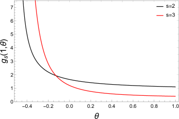
Figure 1: The Dunkl-Bose function versus the Wigner parameter.

We observe that the Dunkl-Bose function decreases as the Wigner parameter increases. Then, we depict the Dunkl-Bose function of $s=3$ for three different Wigner parameters versus $z$ in Fig. 2.

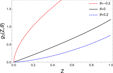
Figure 2: The Dunkl-Bose function, $g_{3}(z,\theta)$, versus $z$ for different Wigner parameters.

We observe that the Dunkl-Bose function is a monotonically increasing function. We see that for a positive value of the Wigner parameter, the Dunkl-Bose function takes smaller values compared to the standard Bose function. For $\theta<0$, this behavior changes oppositely, and the Bose-Dunkl function becomes greater than the usual Bose function. These properties are the characteristic behavior of the functions, and thus, independent of the order $s$.

Now, let us focus on the condensation temperature. We know that when the temperature decreases to the condensation temperature, $T_{c}$, the particles will condense in the ground state of the trap. In such a case of the condensation onset, the system has the state of $N_{0}^{D}\simeq 0$ and $z\simeq 1$. Therefore, we can express the Dunkl-BEC temperature, $T_{c}^{D}$, as

$$T_{c}^{D}\simeq\frac{\hbar\Omega}{k_{B}}\bigg{[}\frac{N}{g_{3}(1,\theta)}\bigg{]}^{1/3}\Bigg{\{}1-\frac{\gamma}{3}\Bigg{[}\frac{g_{2}(1,\theta)}{g_{3}(1,\theta)^{2/3}}\Bigg{]}\frac{1}{N^{1/3}}\Bigg{\}}.$$ (16)

For $\theta=0$, the Dunkl-BEC temperature converts to the traditional critical temperature form, $T_{c}^{B}$, given in [49].

$$T_{c}^{B}\simeq\frac{\hbar\Omega}{k_{B}}\bigg{[}\frac{N}{g_{3}(1)}\bigg{]}^{1/3}\Bigg{\{}1-\frac{\gamma}{3}\Bigg{[}\frac{g_{2}(1)}{g_{3}(1)^{2/3}}\Bigg{]}\frac{1}{N^{1/3}}\Bigg{\}}.$$ (17)

Then, we match Eqs. (16) and (17) to construct a relationship between the latter and the conventional temperatures. We find the ratio

$$\frac{T_{c}^{D}}{T_{c}^{B}}=\left[\frac{\zeta\left(3\right)}{g_{3}(1,\theta)}\right]^{\frac{1}{3}}\frac{1-\frac{\gamma}{3N^{1/3}}\frac{g_{2}(1,\theta)}{g_{3}(1,\theta)^{2/3}}}{1-\frac{\gamma}{18N^{1/3}}\frac{\pi^{2}}{\zeta\left(3\right)^{2/3}}},$$ (18)

where $\zeta\left(n\right)$ is the Riemann-Zeta function. We note that the second term in Eq. (16) can be neglected if the particle number of the ensemble is sufficiently large, $N\rightarrow\infty$. In this case, the Dunkl-BEC temperature can be approximated by $T_{0}^{D}$

$$T_{0}^{D}=\frac{\hbar\Omega}{k_{B}}\left[\frac{N}{g_{3}(1,\theta)}\right]^{\frac{1}{3}},$$ (19)

which reduces to the ordinary case for $\theta=0$ [49]

$$T_{0}^{B}=\frac{\hbar\Omega}{k_{B}}\left[\frac{N}{\zeta\left(3\right)}\right]^{\frac{1}{3}}.$$ (20)

By comparing Eq. (19) with Eq. (20), we get the condensation temperature ratio

$$\frac{T_{0}^{D}}{T_{0}^{B}}=\left[\frac{\zeta\left(3\right)}{g_{3}(1,\theta)}\right]^{\frac{1}{3}}.$$ (21)

We display the change in the condensation temperature ratio versus the Wigner parameter in Fig. 3.

Figure 3: The variation of $\frac{T_{0}^{D}}{T_{0}^{B}}$ versus $\theta$.

We see that this ratio increases with the increasing Wigner parameter value. For the negative Wigner parameter values, this ratio is smaller than one. We see that the ratio saturates at $1.794$ at large Wigner values.

Then, by using Eq. (20) in Eq. (14), we obtain the rate of Dunkl ground state population in terms of normalized temperature as follows:

$$\frac{N_{0}^{D}}{N}=1-\frac{g_{3}(1,\theta)}{\zeta\left(3\right)}\left(\frac{T}{T_{0}^{B}}\right)^{3}-\gamma\frac{g_{2}(1,\theta)}{\zeta^{2/3}\left(3\right)}\frac{1}{N^{1/3}}\left(\frac{T}{T_{0}^{B}}\right)^{2}.$$ (22)

In Fig. 4, we plot this ratio versus the condensation temperature ratio for an ensemble with two thousand particles.

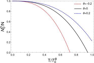
Figure 4: The population of the Dunkl ground state ratio versus normalized temperature for different Wigner parameters.

We see that for positive Wigner parameters, the ground state population of the standard formalism is always smaller than the Dunkl formalism. In other words, for $\theta>0$ the Dunkl-Bosonic system is more apt to undergo a condensation than the standard-Bosonic system. In contrast, for negative values of Wigner parameters, the ground state population in the Dunkl formalism is smaller than the standard formalism.

3 Thermodynamics of the system

At this point, we can employ the internal energy, $U$ to derive the heat capacity function. To obtain the internal energy we substitute the sum with the weighted integral. In this case, the Dunkl internal energy

$$U^{D}=2\int_{0}^{\infty}\frac{E\rho\left(E\right)dE}{e^{2\beta E}z^{-2}-1}+(1+2\theta)\int_{0}^{\infty}\frac{E\rho\left(E\right)dE}{e^{\beta(1+2\theta)E}z^{-(1+2\theta)}+1}.$$ (23)

yields the following result after the substituting Eq. (9) into Eq. (23):

$$\frac{U^{D}}{\hbar\Omega} = 3\left(\frac{k_{B}T}{\hbar\Omega}\right)^{4}g_{4}(z,\theta)+2\gamma\left(\frac{k_{B}T}{\hbar\Omega}\right)^{3}g_{3}(z,\theta).$$ (24)

In order to compute the heat capacity, we have to make a distinction between the two regimes. Below $T_{c}^{D}$, we may safely set $z=1$, however, for $T>T_{c}^{D}$ , we cannot since $z$ is a complicated function of $T$. By using the well-known relation, $C=\partial U/\partial T$, we derive a general expression for the reduced Dunkl heat capacity for $T<T_{c}^{D}$

$$\frac{C_{\leq}^{D}}{Nk_{B}}=12\frac{g_{4}(1,\theta)}{\zeta(3)}\left(\frac{T}{T_{0}^{B}}\right)^{3}+\frac{6\gamma}{N^{1/3}}\frac{g_{3}(1,\theta)}{\zeta^{2/3}(3)}\left(\frac{T}{T_{0}^{B}}\right)^{2}\text{ },$$ (25)

and for $T>T_{c}^{D}$

$$\frac{C_{>}^{D}}{Nk_{B}} =\frac{3}{2}\frac{g_{4}(z,\theta)}{\zeta\left(3\right)}\left(\frac{T}{T_{0}^{B}}\right)^{3}+\frac{3\gamma}{2N^{1/3}}\frac{g_{3}(z,\theta)}{\zeta^{2/3}\left(3\right)}\left(\frac{T}{T_{0}^{B}}\right)^{2}$$

$$+\left[\frac{3}{4}\left(\frac{T}{T_{0}^{B}}\right)^{4}\frac{g_{3}(z,\theta)}{\zeta\left(3\right)}+\frac{\gamma}{N^{1/3}}\frac{g_{2}(z,\theta)}{\zeta^{2/3}\left(3\right)}\left(\frac{T}{T_{0}^{B}}\right)^{3}\right]\frac{T_{0}^{B}}{z}\frac{dz}{dT}.$$ (26)

Here, the quantity $\frac{1}{z}\frac{dz}{dT}$ can be calculated by using the fact that the total particle number is a constant. Considering $\frac{dN}{dT}=0$, we find

$$\frac{T_{0}^{B}}{z}\frac{dz}{dT}=-3\frac{T_{0}^{B}}{T}.\frac{g_{3}(z,\theta)}{g_{2}(z,\theta)}\frac{1+\frac{2\gamma}{3}\frac{\zeta^{1/3}\left(3\right)}{N^{1/3}}\frac{g_{2}(z,\theta)}{g_{3}(z,\theta)}\frac{T_{0}^{B}}{T}}{1+\gamma\frac{\zeta^{1/3}\left(3\right)}{N^{1/3}}\frac{g_{1}(z,\theta)}{g_{2}(z,\theta)}\frac{T_{0}^{B}}{T}},$$ (27)

so that, the Dunkl-specific heat capacity reads

$$\frac{C_{>}^{D}}{Nk_{B}} =\frac{3}{2}\frac{g_{4}(z,\theta)}{\zeta\left(3\right)}\left(\frac{T}{T_{0}^{B}}\right)^{3}+\frac{3\gamma}{2N^{1/3}}\frac{g_{3}(z,\theta)}{\zeta^{2/3}\left(3\right)}\left(\frac{T}{T_{0}^{B}}\right)^{2}$$ (28)

$$-3\frac{g_{3}(z,\theta)}{g_{2}(z,\theta)}\left[\frac{3}{4}\left(\frac{T}{T_{0}^{B}}\right)^{3}\frac{g_{3}(z,\theta)}{\zeta\left(3\right)}+\frac{\gamma}{N^{1/3}}\frac{g_{2}(z,\theta)}{\zeta^{2/3}\left(3\right)}\left(\frac{T}{T_{0}^{B}}\right)^{2}\right]\frac{\frac{T}{T_{0}^{B}}+\frac{2\gamma}{3}\frac{\zeta^{1/3}\left(3\right)}{N^{1/3}}\frac{g_{2}(z,\theta)}{g_{3}(z,\theta)}}{\frac{T}{T_{0}^{B}}+\gamma\frac{\zeta^{1/3}\left(3\right)}{N^{1/3}}\frac{g_{1}(z,\theta)}{g_{2}(z,\theta)}}.$$

Finally, in Fig.5 we plot the Dunkl heat capacity $C_{\leq}^{D}/KN$ versus the temperature $\frac{T}{T_{0}^{B}}$ for different values of Wigner parameters.

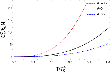
Figure 5: Heat capacity function versus $\frac{T}{T_{0}^{B}}$ of a very large number of bosons in the Dunkl formalism.

We observe that the heat capacity is a monotonically increasing function of $\frac{T}{T_{0}^{B}}$. Therefore, for a fixed value of $\theta$ and $N$, the maximal value of $C_{\leq}^{D}/k_{B}N$ emerges around $T\simeq T_{0}^{B}$. We observe that when considering negative Wigner parameters, the Dunkl heat capacity surpasses the standard heat capacity. Similarly, in the scenario of positive Wigner parameters, the standard formalism exhibits higher values compared to the Dunkl formalism

4 Conclusions

We consider an ideal Bose gas trapped by a three-dimensional anisotropic harmonic oscillator potential in the Dunkl formalism. We derive analytic expressions of the Dunkl-BEC temperature and the Dunkl ground state population and examine the dependence of these quantities on the Wigner parameter. The internal energy and the heat capacity are also computed analytically. The results are shown to nicely generalize known limiting expressions in the non-deformed and/or untrapped cases

Data Availability Statements

The authors declare that the data supporting the findings of this study are available within the article.

References

- [1] V. Bagnato, D. E. Pritchard, and D. Kleppner, Phys. Rev. A 35, 4354 (1987).
- [2] H. A. Gersch, J. Chem. Phys. 27, 928 (1957).
- [3] A. Widom, Phys. Rev. 176, 254 (1968).
- [4] D. B. Baranov and V. S. Yarunin, Phys. Lett. A 285, 34 (2001).
- [5] J. I. Rivas and A. Camacho, Mod. Phys. Lett. A 26, 481 (2011).
- [6] T. G. Liu, Y. Yu, J. Zhao, X. Wang, X. Wang, and Q. H. Liu, Physica A 388, 2383 (2009).
- [7] C. F. Du, H. Li, Z. Q. Lin, and X. M. Kong, Physica B 407, 4375 (2012).
- [8] K. Kirsten, D. J. Toms, Phys. Rev. A 54, 4188 (1996).
- [9] W. Ketterle, and N. J. van Druten, Phys. Rev. A 54, 656 (1996).
- [10] W. J. Mullin, J. Low Temp. Phys. 106, 615 (1997).
- [11] Q. -J. Zeng, Z. Cheng, J. -H. Yuan, Physica A 391, 563 (2012).
- [12] Q. -J. Zeng, Y. -S. Luo, Y. -G. Xu, H. Luo, Physica A 398, 116 (2014).
- [13] W. J. Mullin, A. R. Sakhel, J. Low Temp. Phys. 166, 125 (2011).
- [14] E. P. Wigner, Phys. Rev. 77, 711 (1950).
- [15] L. M. Yang, Phys. Rev. 84, 788 (1951).
- [16] W. S. Chung, and H. Hassanabadi, Eur. Phys. J. Plus 136, 239 (2021).
- [17] C. F. Dunkl, T. Am. Math. Soc. 311(1), 167 (1989).
- [18] R. D. Mota, D. Ojeda-Guill´en, M. Salazar-Ram´Ärez, and V. D. Granados, Mod. Phys. Lett. A 36, 2150171 (2021).
- [19] G. J. Heckman, Prog. Math. 101, 181 (1991).
- [20] C. F. Dunkl, and Y. Xu, Orthogonal Polynomials of Several Variables, Encyclopedia of Mathematics and Its Applications, 81 (Cambridgre: Cambridge University Press) 2001.
- [21] H. de Bie, B. Orsted, P. Somberg, V. Soucek, Trans. Am. Math. Soc. 364, 3875 (2012).
- [22] M. S. Plyushchay, Ann. Phys. 245, 339 (1996).
- [23] S. Kakei, J. Phys. A 29, L619 (1996).
- [24] L. Lapointe, L. Vinet, Commun. Math. Phys. 178(2), 425 (1996).
- [25] M. S. Plyushchay, Nucl. Phys. B 491, 619 (1997).
- [26] M. S. Plyushchay, Int. J. Mod. Phys. A 15, 3679 (2000).
- [27] V. Genest, M. Ismail, L. Vinet, A. Zhedanov, J. Phys. A 46, 145201 (2013).
- [28] V. Genest, L. Vinet, A. Zhedanov, J. Phys. A 46, 325201 (2013).
- [29] V. Genest, M. Ismail, L. Vinet, A. Zhedanov, Commun. Math. Phys. 329, 999 (2014).
- [30] V. Genest, L. Vinet, A. Zhedanov, J. Phys. Conf. Ser. 512, 012010 (2014).
- [31] W. S. Chung, H. Hassanabadi, Mod. Phys. Lett. A 34(24), 1950190 (2019).
- [32] H. Hassanabadi, M. de Montigny, W. S. Chung, P. Sedaghatnia, Physica A 580, 126154 (2021).
- [33] R. D. Mota, D. Ojeda-Guillén, M. Salazar-Ramírez, V. D. Granados, Mod. Phys. Lett. A 36(23), 2150171 (2021).
- [34] W. S. Chung, H. Hassanabadi, Rev. Mex. Fis. 66(3), 308 (2020).
- [35] M. R. Ubriaco, Physica A 414, 128 (2014).
- [36] Y. Kim, W. S. Chung, H. Hassanabadi, Rev. Mex. Fis. 66(4), 411 (2020).
- [37] H. Hassanabadi, M. de Montigny, W. S. Chung, Physica A 580, 126154 (2021).
- [38] S. H. Dong, W. H. Huang, W. S. Chung, P. Sedaghatnia, H. Hassanabadi, EPL 135, 30006 (2021).
- [39] S. Sargolzaeipor, H. Hassanabadi, W. S. Chung, Mod. Phys. Lett. A 33(25), 1850146 (2018).
- [40] S. Ghazouani, I. Sboui, M. A. Amdouni, M. B. El Hadj Rhouma, J. Phys. A: Math. Theor. 52, 225202 (2019).
- [41] R. D. Mota, D. Ojeda-Guillén, M. Salazar-Ramírez, V. D. Granados, Ann. Phys. 411, 167964 (2019).
- [42] B. Hamil, B. C. Lütfüoğlu, Eur. Phys. J. Plus 137, 1241 (2022).
- [43] R. D. Mota, D. Ojeda-Guillén, M. Salazar-Ramírez, V. D. Granados, Mod. Phys. Lett. A 36(10), 2150066 (2021).
- [44] A. Merad, M. Merad, Few-Body Syst. 62, 98 (2021).
- [45] B. Hamil, B. C. Lütfüoğlu, Few-Body Syst. 63, 74 (2022).
- [46] B. Hamil, B. C. Lütfüoğlu, Eur. Phys. J. Plus 137, 812 (2022).
- [47] B. Hamil, B. C. Lütfüoğlu, Physica A 623, 128841 (2023).
- [48] F. Merabtine, B. Hamil, B. C. Lütfüoğlu, A. Hocine, M. Benarous, J. Stat. Mech. 5, 053102 (2023).
- [49] S. Grossmann, M. Holthaus, Phys. Lett. A 208, 188 (1995).