Lorentz-Invariant Interactions in Honeycomb Lattice with Hubbard Interaction

Abstract

We derive Lorentz-invariant four-fermion interactions, including Nambu-Jona-Lasinio type and superconducting type, which are widely studied in high-energy physics, from the honeycomb lattice Hamiltonian with Hubbard interaction. We investigate the phase transitions induced by these two interactions and consider the effects of the chemical potential and magnetic flux (Haldane mass term) on these phase transitions. We find that the charge-density-wave and superconductivity generated by the attractive interactions are mainly controlled by the chemical potential, while the magnetic flux delimits the domain of phase transition. Our analysis underscores the influence of the initial topological state on the phase transitions, a facet largely overlooked in prior studies. We present experimental protocols using cold atoms to verify our theoretical results.

Introduction.– Two-dimensional Dirac materials have emerged as a hot topic in the study of condensed matter physics. The electrons in these materials display a linear dispersion spectrum on the Fermi surface Neto et al. (2009). Despite their fundamentally non-relativistic nature, their low-energy excitations can be described by the (2+1)-dimensional Dirac equation. This intriguing manifestation blurs the traditional boundaries between relativistic and non-relativistic realms in the microscopic world, indicating a possible transformation and connection through specific physical systems. However, the challenge lies in effectively bridging these critical aspects of condensed matter models with theoretical models in high-energy physics, thereby forging a pathway for relativistic studies in condensed matter physics. A particularly promising platform to explore this linkage is the Haldane-Hubbard model, setting the stage for the ensuing discussion in this work.

The Haldane model Haldane (1988), a classical model of topological insulators, has attracted substantial attention Neupert et al. (2011); Read and Green (2000); Xu et al. (2011); Yu et al. (2010); Thonhauser and Vanderbilt (2006). This model describes a two-dimensional honeycomb lattice system with a non-zero Chern number, the characteristics of which have been experimentally verified over the past few years Chang et al. (2013). The Haldane model with interaction has also been extensively studied Herbut (2006); Herbut et al. (2009); Hickey et al. (2016); Vanhala et al. (2016); Cangemi et al. (2019); Yi et al. (2021); Miao et al. (2019); Mai et al. (2023); Yanes et al. (2022); Castro et al. (2023). However, how to connect these essential, experimentally realizable condensed matter models with theoretical models in high-energy physics, and establish a bridge between condensed matter physics and high energy physics, remains an evolving field Herbut and Mandal (2023); Herbut (2023); Palumbo and Pachos (2014, 2013); Cirio et al. (2014). In high-energy physics, four-fermion interactions play a crucial role in describing the properties of strongly interacting particles and understanding the low energy limit of the standard model. For example, the Nambu-Jona-Lasinio (NJL) model and Gross-Neveu (GN) model Fernández et al. (2021, 2020); Alves et al. (2017); Khunjua et al. (2017, 2018, 2019); Ebert et al. (1994); Buballa (2005); Li et al. (2021); Ebert et al. (2001, 2002); Ebert and Klimenko (2010); Ebert et al. (2011, 2014, 2015), are used in the field of particle physics to study meson spectra, color superconductivity, and heavy ion collision physics, etc. And the Thirring model Khunjua et al. (2022); Gubaeva et al. (2022); Gies and Janssen (2010); Gomes et al. (1991), is used to study dynamical symmetry breaking, and the phase diagram of real quantum chromodynamics, etc. Most of these models are phenomenological and lack experimental platforms. However, the unique properties of two-dimensional Dirac materials provide us with a unique opportunity to use these materials to simulate these models in high energy physics, particularly those involving interactions that exhibit Lorentz invariance.

In this Letter, we start from the Haldane model with Hubbard interaction, and through the van der Waerden notation, we first propose a mapping from the honeycomb lattice Hamiltonian to the Lagrangian including two types of interactions: NJL-type and superconducting-type. This notation allows us to transform the non-relativistic Hubbard interaction into these relativistic four-fermion interactions, thereby promoting the construction of a fully Lorentz-invariant Lagrangian. Through the calculation of the effective potential, we study the phase transitions induced by these two interactions. We also examine the effects of the chemical potential and Haldane mass term (magnetic flux) present in the Haldane model on these phase transitions. Finally, we propose to experimentally probe these quantum phase transitions in cold atoms. In the Supplemental Material (SM) sm S-V, we also discuss how the topological properties of the original Haldane model modulate the phase transitions induced by these two four-fermion interactions which has not been studied in any previous literature Ebert et al. (2016); Klimenko et al. (2012); Ebert et al. (2015); Gomes and Ramos (2021, 2023).

Constructing the Lorentz-invariant Lagrangian.– We study a honeycomb lattice system with nearest neighbor interactions, contributing to the following spinless Haldane-Hubbard model:

$$\mathcal{H}=\mathcal{H}_{0}+\mathcal{H}_{T}+\mathcal{H}_{S}+\mathcal{H}_{U}\,,$$ (S1)

with partial Hamiltonian expressed as $\mathcal{H}_{0}=-\sum_{\langle i,j\rangle}t(a_{i}^{\dagger}b_{j}+\text{H.c.})$, $\mathcal{H}_{T}=-\sum_{\langle\langle i,j\rangle\rangle}t^{\prime}(e^{i\phi}a_{i}^{\dagger}a_{j}+e^{-i\phi}b_{i}^{\dagger}b_{j})$, $\mathcal{H}_{S}=\sum_{i\in A}\mu a_{i}^{\dagger}a_{i}-\sum_{i\in B}\mu b_{i}^{\dagger}b_{i}$, $\mathcal{H}_{U}=-\sum_{\langle ij\rangle}Ua^{\dagger}_{i}a_{i}b^{\dagger}_{j}b_{j}$. Here the summation $\sum_{\langle i,j\rangle}$ takes over all nearest-neighbor (NN) sites, and $\sum_{\langle\langle i,j\rangle\rangle}$ takes over all next-nearest-neighbor (NNN) sites. $t$ and $t^{\prime}$ are real-valued NN and NNN hopping amplitudes, and the latter contain addtional phase $\pm\phi$ for different sublattices along the arrows shown in Fig. S1. The particle creation and annihilation operators are denoted by $a^{\dagger}_{i}(b^{\dagger}_{i})$ and $a_{i}(b_{i})$ for A(B) sublattice. The energy offset $\mu$ between sites of A-B sublattices breaks inversion symmetry. $U$ denotes the NN interaction strength between particles in different sublattices. In the following we explain how the Haldane model can be associated with free dirac fermion Lagrangian, and gives an exact mapping from the Hubbard interaction to those Lorentz invariant four-fermion interactions. We will propose to realize such a Lorentz-invariant four-fermion model and detect the predicted phases using ultracold atoms (see SM sm S-VI).

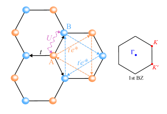
Figure S1: Haldane model on a honeycomb lattice with nearest neighbor interactions. The sublattices A and B are represented by orange and blue sites, respectively, each with an energy offset denoted by $\mu$. The real isotropic values are characterized by nearest-neighbor (NN) hopping terms $t$. The next-nearest-neighbor (NNN) hopping $t^{\prime}$ is indicated by dashed lines with arrows, incorporating a phase factor $e^{\pm i\phi}$. The interaction $U$ is observed between adjacent particles. The diagram in the right delineates the Brillouin zone, featuring the Dirac points $K$ and $K^{\prime}$.

We focus on the NN hopping Hamiltonian $\mathcal{H}_{0}$. From the dispersion relation for the noninteracting theory we obtain six $K$ points, and our choice of two inequivalent ones, which we denote $K_{\pm}$, these correspond to the $K$ and $K^{\prime}$ points in Fig. S1. Expanding around $K_{\pm}$, the Hamiltonian $\mathcal{H}_{0}$ becomes: $H_{0}\!=\!\int\!\frac{d^{2}p}{(2\pi)^{2}}(\psi_{+}^{\dagger}(p)v_{F}\sigma\cdot p\psi_{+}(p)\!-\!v_{F}\psi_{-}^{\dagger}(p)\left(p_{x}\sigma_{x}-p_{y}\sigma_{y}\right)\psi_{-}(p))$, where $\psi_{\pm}(p)\!=\!(a(K_{\pm}+p),b(K_{\pm}+p))^{\intercal}$, $v_{F}=3td/2$ ($d$ is the lattice constant). And afterwards, for convenience, we will denote $a(K_{\pm}+p)$ by $a_{\pm}$, and $b(K_{\pm}+p)$ by $b_{\pm}$.

We encapsulate the Hamiltonian of point $K$ and point $K^{\prime}$ inside a four-component spinor $\Psi^{\intercal}=\left(a_{+},b_{+},b_{-},a_{-}\right)$. After using the Legendre transformation we can obtain the Lagrangian of the system: $\mathcal{L}=\bar{\Psi}\left(i\gamma^{v}\partial_{v}\right)\Psi$. where $\bar{\Psi}=\Psi^{\dagger}\gamma^{0}$, $v=0,1,2$ and we set $v_{F}=1$ for convenience. We use the irreducible four-dimensional spinor representation, the gamma matrices are $\gamma^{\mu}=\left(\begin{array}[]{cc}0&\bar{\sigma}^{\mu}\\ \sigma^{\mu}&0\end{array}\right)$ and $\mu=0,1,2,3$. There exist one other matrice $\gamma^{5}=\left(\begin{array}[]{cc}1&0\\ 0&-1\end{array}\right)$, which anticommute with all $\gamma^{\mu}$ sm . We now consider the NNN hopping $\mathcal{H}_{T}$ and the chemical potential term $\mathcal{H}_{S}$. The effective Lagrangian obtained by expanding $\mathcal{H}_{T}+\mathcal{H}_{S}$ at the Dirac point $K,K^{\prime}$ are $\mathcal{L}_{m}=\psi_{\pm}^{\dagger}m_{\pm}\sigma_{z}\psi_{\pm}$. Where $m_{\pm}=\mu\pm 3\sqrt{3}t^{\prime}\sin\phi$. For convenience, we set $m_{o}=3\sqrt{3}t^{\prime}\sin\phi$, and it is actually the Haldane mass term Carrington (2019); Dudal et al. (2018); Gusynin et al. (2007). Now, encapsulate it inside the four-component spinor, we can get the on-site and Haldane mass terms respectively: $\mu\bar{\Psi}\gamma^{3}\Psi$, $m_{o}\bar{\Psi}\gamma^{3}\gamma^{5}\Psi$ sm . Finally, we can get the free Dirac fermion Lagrangian from the effective theory of Haldane model is: $\mathcal{L}=\bar{\Psi}\left(i\gamma^{v}\partial_{v}+\mu\gamma^{3}+m_{o}\gamma^{3}\gamma^{5}\right)\Psi$ .

We now consider the Hubbard interaction $H_{U}$ in continue limit and ignore the interaction between $K$ and $K^{\prime}$ Luo et al. (2015a, b). We take into account the Hubbard interaction for both $K$ and $K^{\prime}$ point, i.e., $H_{U}\approx H_{int}\equiv\int d{\bf r}\ U(a_{+}^{\dagger}a_{+}b_{+}^{\dagger}b_{+}+a_{-}^{\dagger}a_{-}b_{-}^{\dagger}b_{-})$ . Following, we’ll use the van der Waerden notation to map the $H_{int}$ to the Lorentz invariant four-fermion interactions, which contain NJL-type and Superconducting-type. Below we will demonstrate how to create this mapping. We note that $\Psi=\left(\begin{array}[]{l}\psi_{+}\\ \sigma_{1}\psi_{-}\end{array}\right)$, and for convenience we define $\chi=\sigma_{1}\psi_{-}$ and $\eta=\psi_{+}$. Actually, $\eta$ is the right-chiral weyl spinor, and the corresponding $\chi$ is the left-chiral spinor. Thus, $\Psi$ is indeed a Dirac spinor containing two different chiral weyl spinors, i.e., $\Psi=\left(\begin{array}[]{l}\eta\\ \chi\end{array}\right)$. We introduce the van der Waerden notation and since we are using the path integral framework, the elements inside $\Psi$ are grassman numbers rather than operators. According to this notation Muller-Kirsten and Wiedemann (2010); Labelle (2010); Martin (2010), we have $\chi_{1}=b_{-},\;\chi_{2}=a_{-},\;\chi^{a}=\epsilon^{ab}\chi_{b},\;\bar{\eta}^{\dot{1}}=a_{+},\;\bar{\eta}^{\dot{2}}=b_{+},\;\bar{\eta}^{\dot{a}}=\epsilon^{\dot{a}\dot{b}}\bar{\eta}_{\dot{b}}$, where $\epsilon^{12}=\epsilon^{\dot{1}\dot{2}}=1$ and $\epsilon_{12}=\epsilon_{\dot{1}\dot{2}}=-1$. We use the notation $\chi\cdot\chi\equiv\chi^{a}\chi_{a}=\chi^{\intercal}(-i\sigma_{2})\chi$ and $\bar{\chi}\cdot\bar{\chi}\equiv\bar{\chi}_{\dot{a}}\bar{\chi}^{\dot{a}}=\chi^{\dagger}i\sigma_{2}\chi^{\dagger\intercal}$, which are invariant under Lorentz transformation. The Hamiltonian density of the Hubbard interaction can be expressed as: $4a_{+}^{\dagger}a_{+}b_{+}^{\dagger}b_{+}\!=\!(\eta\cdot\eta)(\bar{\eta}\cdot\bar{\eta})$. Similarly, $4a_{-}^{\dagger}a_{-}b_{-}^{\dagger}b_{-}\!=\!(\bar{\chi}\cdot\bar{\chi})(\chi\cdot\chi)$. We then introduce a charge conjugate operator $C=-i\gamma^{2}\gamma^{0}$ which satisfies $C=-C^{-1}=-C^{\dagger}$. So, the Hubbard interaction finally can be mapped to the Lorentz invariant four-fermion interactions: $H_{int}\!=\!\frac{U}{4}[(\Psi^{\intercal}C\Psi)(\bar{\Psi}C\bar{\Psi}^{\intercal})\!+\!(\bar{\Psi}\Psi)^{2}\!-\!(\bar{\Psi}i\gamma^{5}\Psi)^{2}]$ sm .

In the following, we discuss the properties of the model in a more general sense, i.e., using the following Lagrangian:

$$\mathcal{L} =\sum_{i}\bar{\Psi}_{i}\left(i\gamma^{v}\partial_{v}+\mu\gamma^{3}+m_{o}\gamma^{3}\gamma^{5}\right)\Psi_{i}$$

$$+\frac{G_{1}}{N}[(\sum_{i}\bar{\Psi}_{i}\Psi_{i})^{2}-(\sum_{i}\bar{\Psi}_{i}i\gamma^{5}\Psi_{i})^{2}]$$

$$+\frac{G_{2}}{N}(\sum_{i}\Psi^{\intercal}_{i}C\Psi_{i})\sum_{j}(\bar{\Psi}_{j}C\bar{\Psi}^{\intercal}_{j})\,.$$ (S2)

Here, we have adopted the large-N assumption that all fermion fields $\Psi_{i}(i=1,...,N)$ form a fundamental multiplet of the $O(N)$ group. This model is similar to those investigated in Refs. Ebert et al. (2016); Klimenko et al. (2012); Ebert et al. (2015); Gomes and Ramos (2021, 2023), but we consider the effect of the haldane mass term, an aspect not addressed in these references. Our assumption $G_{1}=G_{2}=\frac{U}{4}$ are derived from Hubbard interaction rather than a direct phenomenological parameter, and all the order parameters representing phases that we discuss subsequently originate from genuine condensed matter systems. It is worth mentioning that in this Letter, we adopt a distinct gamma matrix representation. However, as we will demonstrate below, the physical results are independent of the representation chosen for the gamma matrices. And in the main text, we will only consider the parts that are directly related to the Hubbard interaction, i.e., $G_{1}=G_{2}=G$.

Effective potential.– We use the Hubbard-Stratonovich (HS) transformation to decouple these four-fermion interactions and solve for the thermodynamic potential (TDP). We focus on the case with Hubbard interaction, where we set $G_{1}=G_{2}=G$ and $G=U/4$. Introducing the auxiliary fields $\Delta,\pi,\sigma$, we have $\mathcal{L}=\bar{\Psi}_{i}\left(i\gamma^{v}\partial_{v}+\mu\gamma^{3}+m_{o}\gamma^{3}\gamma^{5}-\sigma-i\gamma^{5}\pi\right)\Psi_{i}$ $-\frac{N}{4G}(\sigma^{2}+\pi^{2})-\frac{N}{4G}\Delta^{\ast}\Delta-\frac{\Delta^{\ast}}{2}\Psi^{\intercal}_{i}C\Psi_{i}-\frac{\Delta}{2}\bar{\Psi}_{i}C\bar{\Psi}^{\intercal}_{i}$. Using the Euler-Lagrange equations of motion for these auxiliary fields which take the form: $\sigma(x)=-2\frac{G}{N}(\bar{\Psi}_{i}\Psi_{i})$, $\pi(x)=-2\frac{G}{N}(\bar{\Psi}_{i}i\gamma^{5}\Psi_{i})$ and $\Delta(x)=-2\frac{G}{N}(\Psi_{i}^{\intercal}C\Psi_{i})$. The ground state expectation values $\langle\Delta(x)\rangle,\langle\pi(x)\rangle,\langle\sigma(x)\rangle$ of the composite bosonic fields are determined by the saddle point equations $\frac{\delta{\cal S}_{\rm{eff}}}{\delta\sigma(x)}=0,\;\frac{\delta{\cal S}_{\rm{eff}}}{\delta\Delta(x)}=0,\;\frac{\delta{\cal S}_{\rm{eff}}}{\delta\pi(x)}=0$. Where $\exp(i{\cal S}_{\rm{eff}}(\sigma,\Delta,\Delta^{*}))=\int\prod_{l=1}^{N}[d\bar{\psi}_{l}][d\psi_{l}]\exp\Bigl(i\int{\cal L}\,d^{3}x\Bigr{missing})$. For simplicity, throughout the paper we suppose that the above mentioned ground state expectation values do not depend on space-time coordinates: $\vev{\sigma(x)}\equiv\sigma$, $\vev{\pi(x)}\equiv\pi$, $\vev{\Delta(x)}\equiv\Delta$. So, in the leading order of the large-$N$ expansion, after integrating out the fermionic field, we can derive the TDP:

$$\Omega=\frac{\sigma^{2}+\pi^{2}}{4G}+\frac{\Delta^{2}}{4G}+\frac{i}{2}\sum_{i}\int\frac{d^{3}p}{(2\pi)^{3}}log\lambda_{i}(p)\,,$$ (S3)

where $\Delta$ is a real number, $\lambda_{i}(p)$($i=1,2,3,4$) is the four roots of the four-by-four matrix $\mathcal{D}(p)=-\Delta^{2}\bf{I}+\mathcal{D}_{+}\mathcal{D}_{-}$ sm . Without loss of generality, for chiral symmetry breaking, we can always choose a direction such that $\pi=0,\sigma\neq 0$. In powers of $p_{0}$, we can write $\prod_{i}\lambda_{i}(p)=P^{+}(p_{0})P^{-}(p_{0})$. According to the general theorem of algebra, the polynomial $P^{\beta}(p_{0})$($\beta=+,-$) can be presented in the form: $P^{\beta}(p_{0})=(p_{0}-p^{\beta}_{01})(p_{0}-p^{\beta}_{02})(p_{0}-p^{\beta}_{03})(p_{0}-p^{\beta}_{04})$. Then, the TDP is: $\Omega=\frac{\sigma^{2}}{4G}+\frac{\Delta^{2}}{4G}+\frac{i}{2}\sum_{\beta}\int\frac{d^{3}p}{(2\pi)^{3}}logP^{\beta}(p_{0})$. Using the general formula: $\int_{-\infty}^{\infty}dp_{0}\ln\big(p_{0}-R)=\mathrm{i}\pi|R|$. Where R is a real quantity, it is possible to reduce the TDP to the following: $\Omega\equiv\Omega^{un}(\Delta,\sigma)=\frac{\sigma^{2}}{4G}+\frac{\Delta^{2}}{4G}-\frac{1}{4}\sum_{\beta,i}\int\frac{d^{2}\bm{p}}{(2\pi)^{2}}(|p^{\beta}_{0i}|)$.

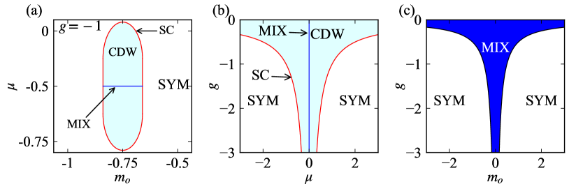
Figure S2: The phase diagrams of the system under various fixed parameters: (a) The phase diagram in the $(\mu,m_{o})$ parameter space, where the interaction strength $g=-1$. (b) The phase diagram in the $(g,\mu)$ parameter space, where the Haldane mass term $m_{o}=0$. (c) The phase diagram in the $(g,m_{o})$ parameter space, where the chemical potential $\mu=0$. In the diagrams, the white area denotes the system in a symmetry (SYM) phase, the sky-blue area represents the system in a CDW phase, the red area indicates the system is in a superconductor (SC) phase, and the blue area signifies the system is in a mixed (MIX) phase of CDW and superconductivity.

Renormalization and phase diagram.– First, we will obtain a finite (i.e., renormalized) expression for the TDP at $m_{o}=0$ and $\mu=0$. That is, in vacuum: $V^{un}(\Delta,\sigma)=\frac{\sigma^{2}}{4G}+\frac{\Delta^{2}}{4G}-\int\frac{d^{2}\bm{p}}{(2\pi)^{2}}(\sqrt{\bm{p}^{2}+(\Delta+\sigma)^{2}}+\sqrt{\bm{p}^{2}+(\Delta-\sigma)^{2}})$. Next, let us regularize the effective potential by cutting momenta; we suppose that $|\bm{p}|<\Lambda$. (Note here that we take a spherical coordinate truncation instead of the square truncation in Ref. Ebert et al. (2016), so there is a difference in the sense of constants). As a result, we have the following regularized expression, which is finite at finite values of $\Lambda$:

$$V^{un}(\Delta,\sigma) =(\sigma^{2}+\Delta^{2})(\frac{1}{4G}-\frac{\Lambda}{2\pi})-\frac{\Lambda^{3}}{3\pi}$$

$$+\frac{1}{6\pi}(|\Delta+\sigma|^{3}+|\Delta-\sigma|^{3})\,.$$ (S4)

We assume that the bare coupling constants $G$ depend on the cutoff parameter of $\Lambda$ in the way that in the limit $\Lambda\to\infty$ yields a finite expression in square brackets (Lorentz-Invariant Interactions in Honeycomb Lattice with Hubbard Interaction) . Obviously, in order to satisfy this requirement, it is sufficient to require that $\frac{1}{4G}\equiv\frac{1}{4G(\Lambda)}=\frac{\Lambda}{2\pi}+\frac{1}{2\pi g}$. where $g$ is finite and $\Lambda$-independent model parameter with dimensionality of inverse mass. Ignore there an infinite $\sigma$- and $\Delta$-independent constant $-\frac{\Lambda^{3}}{3\pi}$, one obtains the following renormalization, i.e., finite expression for the effective potential: $V^{ren}(\Delta,\sigma)=\lim_{\Lambda\to\infty}\left\{V^{un}(\Delta,\sigma)\Big{|}_{G(\Lambda)}+\frac{\Lambda^{3}}{3\pi}\right\}$. It should also be mentioned that the $V^{ren}$ is a renormalization group invariant quantity. Finally, we get $V^{ren}(\Delta,\sigma)=\frac{\sigma^{2}}{2\pi g}+\frac{\Delta^{2}}{2\pi g}+\frac{1}{6\pi}(|\Delta+\sigma|^{3}+|\Delta-\sigma|^{3})$. The coordinates of the global minimum point $(\Delta_{0},\sigma_{0})$ of the effective potential $V^{ren}(\Delta,\sigma)$ define the ground state expectation values of auxiliary fields $\sigma(x)$ and $\Delta(x)$. Namely, $\sigma_{0}=\vev{\sigma(x)}$ and $\Delta_{0}=\vev{\Delta(x)}$. The quantities $\sigma_{0}$ and $\Delta_{0}$ are usually called order parameters, or gaps. Moreover, the gap $\sigma_{0}$ is equal to the dynamical mass of one-fermionic excitations of the ground state. That is, its appearance is associated with chiral symmetry breaking. In this work, originating from genuine condensed matter systems, the specific pairing of $\sigma$ arises from the particle-hole pairing located at two inequivalent Dirac points, leading to the charge-density-wave (CDW) sm . The emergence of $\Delta_{0}$ is associated with the onset of the superconducting phase transition. It is worth noting that although the regularization scheme we adopt and the representation of the gamma matrix are different from those in Ref. Ebert et al. (2016), the final resulting effective potential is indeed precisely the same, so does the phase portrait. This demonstrates that the effective potential is indeed a renormalization group invariant quantity, and it confirms that the physics of the system is independent of the representation chosen for the gamma matrices.

We now study the influence of the Haldane mass term $m_{o}$ and the chemical potential $\mu$ on the phase structure of the model. We have sm

$$\Omega^{ren}(\Delta,\sigma)=\frac{\sigma^{2}}{2\pi g}+\frac{\Delta^{2}}{2\pi g}+\frac{1}{12\pi}(|\Delta+m_{o}+\sqrt{\mu^{2}+\sigma^{2}}|^{3}$$

$$+|\Delta+m_{o}-\sqrt{\mu^{2}+\sigma^{2}}|^{3}+|\Delta-m_{o}+\sqrt{\mu^{2}+\sigma^{2}}|^{3}$$

$$+|\Delta-m_{o}-\sqrt{\mu^{2}+\sigma^{2}}|^{3}).$$ (S5)

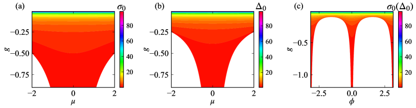
Figure S3: Thermal diagrams of order parameters versus interaction $g$ and chemical potential $\mu$ or magnetic flux $\phi$ (Haldane mass $m_{o}$), respectively. (a,b) Thermal diagrams of the order parameters $\sigma_{0}$, $\Delta_{0}$ in the parameter space ($g,\mu$), respectively. (c) Thermal diagrams of the order parameters $\sigma_{0}$, $\Delta_{0}$ in the parameter space ($g,\phi$), where $\sigma_{0}=\Delta_{0}$.

By solving the extreme points of the given TDP, we can derive the system’s phase diagram, which is determined by the interplay of three parameters ($g,\mu,m_{o}$). We find that in the repulsive region ($g>0$), no spontaneous symmetry breaking occurs. Conversely, in the attractive region ($g<0$), the system undergoes spontaneous symmetry breaking, leading to a transition from the CDW to superconductivity. Interestingly, the region exhibiting superconductivity is quite peculiar, manifesting only at the phase boundary. And the chemical potential $\mu$ plays a pivotal role in inducing transitions to both the superconducting phase and the CDW. Meanwhile, the Haldane mass term merely triggers the system’s transition process from a symmetric phase to a mixed phase. The corresponding phase diagrams are shown in Fig. S2.

We know that the Haldane model is a topological insulator, characterized by the Chern number $C=\frac{1}{2}(\text{sgn}(\mu+m_{o})-\text{sgn}(\mu-m_{o}))$. Interestingly, $C$ is determined by the chemical potential $\mu$ and the Haldane mass term $m_{o}$. This raises the question: is the phase transition of this system related to its topology? Inspection of Fig. S2 (a), where the interactions are set to $g_{1}=g_{2}=g$, reveals no direct correlation between the system’s topology and its phase transitions. However, in the SM sm S-V, we investigated the phase diagram of the $(g_{1},g_{2})$ system in different topological states, and discovered that the topology plays a role in determining the phase boundaries.

Lastly, we plotted the phase diagrams of the $(g,m_{o})$ and $(g,\mu)$ systems, where $(\mu=0,m_{o}=0)$ correspond to Fig. S2 (b and c), and the equations of the corresponding boundary curves of these two plots are $g=-\frac{1}{|\mu|}$ and $g=-\frac{1}{2|m_{o}|}$, respectively. We find that when $\mu=0$, under attractive interaction, tuning $m_{o}$ from negative to positive leads the system to undergo phase transitions from symmetric phase to mixed phase and back to symmetric phase. On the other hand, at $m_{o}=0$, adjusting the chemical potential $\mu$ induces the system to experience phase transitions from a symmetry phase to a superconducting phase, followed by the emergence of CDW (apart from the line at $\mu=0$, where the system is in a mixed phase) and then back to symmetry. This suggests that the chemical potential $\mu$ strongly induces the emergence of CDW in the system, while the Haldane mass term merely restricts the range of symmetry breaking. In the SM sm S-IV, we also draw the phase diagrams for ($g,\mu$) and ($g,m_{o}$) with $m_{o}$ and $\mu$ not equal to 0, respectively. In order to compare with the experiment, we also plotted the order parameters as a function of magnetic flux and chemical potential, see Fig. S3, where (a) and (b) is the thermal diagrams of $\sigma_{0}(g,\mu)=\sqrt{1/g^{2}-\mu^{2}}$ and $\Delta_{0}(g,\mu)=\frac{-1/g+\sqrt{1/g^{2}-4\mu^{2}}}{2}$, respectively ($m_{o}=0$ in this case). (c) is the thermal diagrams of $\sigma_{0}(g,\phi)=\Delta_{0}(g,\phi)=\frac{-1/g+\sqrt{1/g^{2}-4(3\sqrt{3}t\sin\phi)^{2}}}{2}$ (where we have set $t=1$ and $\mu=0$).

Discussion and conclusions.– We leverage the van der Waerden notation, widely used in supersymmetric spinor calculations, to map the low-energy effective Hamiltonian of the Haldane model with Hubbard interaction onto a Lorentz-invariant Lagrangian featuring four-fermion interactions. By solving this model, we unveil two distinct phases: superconducting phase and CDW phase, both driven by the Hubbard interactions. Through this mapping, we establish a bridge between high-energy and condensed matter physics, where bilinear quantities and four-Fermi terms in the Lorentz-invariant Lagrangian can be derived in real condensed matter systems, facilitating the emulation of high-energy phenomena in condensed matter systems.

Looking forward, there are several promising avenues for future research. Investigating other two-dimensional lattice models with topological properties Sun et al. (2013); Sun and Ye (2023a, b); Klipstein (2021); Chen et al. (2015); Zhao et al. (2021); Li et al. (2020, 2017); Lee and Qi (2014); Zhang et al. (2014); Yang et al. (2019) and exploring their connection to high-energy physics through similar mapping techniques would provide a broader understanding of the interplay between topology and phase transitions in various systems. Extending our approach to systems with more complex interactions such as long-range couplings could shed light on the emergence of exotic phases and help identify novel materials with unique properties for potential applications in quantum information and nanotechnology. Acknowledgements.– This work was supported by National Key R&D Program of China under grants No. 2021YFA1400900, 2021YFA0718300, 2021YFA1402100, NSFC under grants Nos. 61835013, 12174461, 12234012, Space Application System of China Manned Space Program.

S-I Supplemental Material

S-I.1 Algebra of the $\gamma$ matrices

Given that the two spinors in graphene, which are expanded at two inequivalent Dirac points, correspond to left and right-handed fermions respectively, we adopt the so-called Weyl representation for our gamma algebra here Peskin (2018); Srednicki (2007):

$$\gamma^{\mu}=\left(\begin{array}[]{ll}0&\bar{\sigma}^{\mu}\\ \sigma^{\mu}&0\end{array}\right),$$ (S6)

where $\mu=0,1,2,3$ and $\bar{\sigma}^{\mu}=\sigma^{\mu}$ when $\mu=0$ and $\bar{\sigma}^{\mu}=-\sigma^{\mu}$ when $\mu=1,2,3$ (where $\sigma_{0}$ is the unit 2 $\times$ 2 matrix $I$). These gamma matrix have the properties: $\{\gamma^{\mu},\gamma^{\nu}\}=2g^{\mu\nu}$,where $g^{\mu\nu}=g_{\mu\nu}=diag(1,-1,-1,-1)$. There exist another matrices $\gamma^{5}$, which anticommute with all $\gamma^{\mu}$:

$$\gamma^{5}=i\gamma^{0}\gamma^{1}\gamma^{2}\gamma^{3}=\left(\begin{array}[]{ll}-I&0\\ 0&I\end{array}\right).$$ (S7)

Trace of $\gamma$ matrices can be evaluated as follows:

$$\operatorname{tr}(\mathbf{1}) =4,$$ (S8)

$$\operatorname{tr}\left(\text{ any odd }\gamma^{\prime}\mathrm{s}\right) =0,$$

$$\operatorname{tr}\left(\gamma^{\mu}\gamma^{\nu}\right) =4g^{\mu\nu},$$

$$\operatorname{tr}\left(\gamma^{\mu}\gamma^{\nu}\gamma^{\rho}\gamma^{\sigma}\right) =4\left(g^{\mu\nu}g^{\rho\sigma}-g^{\mu\rho}g^{\nu\sigma}+g^{\mu\sigma}g^{\nu\rho}\right),$$

$$\operatorname{tr}\left(\gamma^{5}\right) =0,$$

$$\operatorname{tr}\left(\gamma^{\mu}\gamma^{\nu}\gamma^{5}\right) =0,$$

$$\operatorname{tr}\left(\gamma^{\mu}\gamma^{\nu}\gamma^{\rho}\gamma^{\sigma}\gamma^{5}\right) =-4i\epsilon^{\mu\nu\rho\sigma}.$$

Contractions of $\gamma$ matrices with each other simplify to:

$$\gamma^{\mu}\gamma_{\mu} =4,$$ (S9)

$$\gamma^{\mu}\gamma^{\nu}\gamma_{\mu} =-2\gamma^{\nu},$$

$$\gamma^{\mu}\gamma^{\nu}\gamma^{\rho}\gamma_{\mu} =4g^{\nu\rho},$$

$$\gamma^{\mu}\gamma^{\nu}\gamma^{\rho}\gamma^{\sigma}\gamma_{\mu} =-2\gamma^{\sigma}\gamma^{\rho}\gamma^{\nu}.$$

S-I.2 Performing the path integral over the fermion

Let us show here some of the details of the path integral over the fermions and which leads to the effective thermodynamic potential. Adopting the procedure described in Refs.  Ebert et al. (2016); Klimenko et al. (2012), we assume two anti-commuting four component Dirac spinor fields $q(x)$ and $\bar{q}(x)$. Then,we’ll calculate the following path integral:

$$I = \int DqD\bar{q}~{}e^{i\int d^{3}x\left[\bar{q}\mathcal{D}q-\frac{\Delta^{*}}{2}q^{\intercal}Cq-\frac{\Delta}{2}\bar{q}C\bar{q}^{\intercal}\right]},$$ (S10)

where $\mathcal{D}=i\gamma_{\mu}\partial_{\nu}+\mu\gamma^{3}+m_{o}\gamma^{3}\gamma^{5}-\sigma-i\pi\gamma^{5}$ and $C=-i\gamma^{2}\gamma^{0}$ is the charge conjugation matrix. Using the Gaussian path integral identities

$$\int Dpe^{i\int d^{3}x\Big{[}-\frac{1}{2}p^{\intercal}Ap+\eta^{\intercal}p\Big{]}}=(\det A)^{1/2}e^{-\frac{i}{2}\int d^{3}x\eta^{\intercal}A^{-1}\eta}~{},$$ (S11)

and

$$\int D\bar{p}e^{i\int d^{3}x\Big{[}-\frac{1}{2}\bar{p}A\bar{p}^{\intercal}+\eta\bar{p}^{\intercal}\Big{]}}=(\det A)^{1/2}e^{-\frac{i}{2}\int d^{3}x\bar{\eta}A^{-1}\bar{\eta}^{\intercal}},$$ (S12)

and by also considering $A=\Delta C$, $\bar{q}\mathcal{D}=\eta^{\intercal}$, $\mathcal{D}^{\intercal}\bar{q}^{\intercal}=\eta$, one finds, after integrating over $q$ and $\bar{q}$, the result

$$I=\int DqD\bar{q}~{}e^{i\int d^{3}x\Bigg{[}\bar{q}\mathcal{D}q-\frac{\Delta^{*}}{2}q^{\intercal}Cq-\frac{\Delta}{2}\bar{q}C\bar{q}^{\intercal}\Bigg{]}}=\left[\det\left(\Delta^{2}C^{2}+\mathcal{D}C^{-1}\mathcal{D}^{\intercal}C\right)\right]^{\frac{1}{2}},$$ (S13)

where we have assumed $\Delta=\Delta^{*}$ in the last step . Using the relations $C^{-1}\gamma_{\mu}^{\intercal}C=-\gamma_{\mu}$ ($\mu=0,1,2,3$) and $\partial_{\mu}^{\intercal}=-\partial_{\mu}$ one finds that

$$I=[\det(-\Delta^{2}+\mathcal{D}_{+}\mathcal{D}_{-})]^{1/2}=(\det B)^{\frac{1}{2}},$$ (S14)

with $\mathcal{D}_{\pm}=i\gamma_{\mu}\partial_{\nu}+m_{o}\gamma^{3}\gamma^{5}-\sigma-i\pi\gamma^{5}\pm\mu\gamma^{3}$. Finally, using the identity $\det B=\exp({\rm Tr}\ln B)$ one finds

$$\ln I=\frac{1}{2}{\rm Tr}(\ln B)=\int d^{3}x\sum_{i}\int\frac{d^{3}p}{(2\pi)^{3}}\ln\lambda_{i}(p),$$ (S15)

$\lambda_{i}(p)$ are the eigenvalues of matrix $B(p)$.

$$B(p) =-\Delta^{2}+(p_{\mu}\gamma^{\mu}+m_{o}\gamma^{3}\gamma^{5}-\sigma-i\gamma^{5}\pi+\mu\gamma^{3})\times(p_{\mu}\gamma^{\mu}+m_{o}\gamma^{3}\gamma^{5}-\sigma-i\gamma^{5}\pi-\mu\gamma^{3})$$ (S16)

$$=p^{2}-\Delta^{2}+m_{o}^{2}+\sigma^{2}+\mu^{2}-2\sigma\not{p}-2\sigma m_{o}\gamma^{3}\gamma^{5}+2m_{o}\not{p}\gamma^{3}\gamma^{5}-2\mu\not{p}\gamma^{3}-2m_{o}\mu\gamma^{5},$$

where $\not{p}=p^{\mu}\gamma_{\mu}$. In our analysis, we first consider the integration over the frequency component $p_{0}$. The eigenvalues $\lambda_{i}$ of the matrix $B(p)$ can be expressed as a polynomial in terms of $p_{0}$ as follows:

$$\lambda_{i}(p)=p_{0}-\widetilde{\lambda_{i}}({\bf p}),$$ (S17)

where

$$\widetilde{\lambda_{i}}({\bf p})=\left\{\begin{array}[]{l}\pm\sqrt{{\bf p}^{2}+(\Delta+m_{o}+\beta\sqrt{\mu^{2}+\sigma^{2}})^{2}},\\ \pm\sqrt{{\bf p}^{2}+(\Delta-m_{o}-\beta\sqrt{\mu^{2}+\sigma^{2}})^{2}},\end{array}\right.$$ (S18)

and $\beta=\pm$. This implies that $p_{0}$ has a total of eight roots.

To integrate the frequency part of Eq. (S15), we employ the formula $\int_{-\infty}^{\infty}dp_{0}\ln\big(p_{0}-R)=\mathrm{i}\pi|R|$, yielding:

$$\ln I=i\int d^{3}x\sum_{\beta}\int\frac{d^{2}{\bf p}}{(2\pi)^{2}}\left(|\sqrt{{\bf p}^{2}+(\Delta+m_{o}+\beta\sqrt{\mu^{2}+\sigma^{2}})^{2}}|+|\sqrt{{\bf p}^{2}+(\Delta-m_{o}-\beta\sqrt{\mu^{2}+\sigma^{2}})^{2}}|\right).$$ (S19)

From this, we can derive the unrenormalized thermodynamic potential (TDP) as:

$$\Omega\equiv\Omega^{un}(\Delta,\sigma)=\frac{\sigma^{2}}{4G}+\frac{\Delta^{2}}{4G}-\frac{1}{4}\sum_{\beta,i}\int\frac{d^{2}{\bf p}}{(2\pi)^{2}}|p^{\beta}_{0i}|,$$ (S20)

where $p_{0,1}^{\beta}=\sqrt{{\bf p}^{2}+(\Delta+m_{o}+\beta\sqrt{\mu^{2}+\sigma^{2}})^{2}}$ and $p_{0,2}^{\beta}=\sqrt{{\bf p}^{2}+(\Delta-m_{o}-\beta\sqrt{\mu^{2}+\sigma^{2}})^{2}}$.

To renormalize the TDP, we use the following formula:

$$\Omega^{un}(\Delta,\sigma,\mu,m_{o}) =\frac{\sigma^{2}}{4G}+\frac{\Delta^{2}}{4G}-\int\frac{d^{2}{\bf p}}{(2\pi)^{2}}\left(\sqrt{{\bf p}^{2}+(\Delta+\sigma)^{2}}+\sqrt{{\bf p}^{2}+(\Delta-\sigma)^{2}}\right)$$ (S21)

$$-\frac{1}{4}\sum_{\beta,i}\int\frac{d^{2}{\bf p}}{(2\pi)^{2}}\left(|p^{\beta}_{0i}|-4\left(\sqrt{{\bf p}^{2}+(\Delta+\sigma)^{2}}+\sqrt{{\bf p}^{2}+(\Delta-\sigma)^{2}}\right)\right)$$

$$=V^{un}(\Delta,\sigma)-\frac{1}{4}\sum_{\beta,i}\int\frac{d^{2}{\bf p}}{(2\pi)^{2}}\left(|p^{\beta}_{0i}|-4\left(\sqrt{{\bf p}^{2}+(\Delta+\sigma)^{2}}+\sqrt{{\bf p}^{2}+(\Delta-\sigma)^{2}}\right)\right).$$

The second term on the right-hand side of the above equation is finite, so the renormalization of $\Omega$ depends only on the renormalization of the first term. As we have derived in the main text, the renormalized potential is given by $V^{ren}(\Delta,\sigma)=\frac{\sigma^{2}}{2\pi g}+\frac{\Delta^{2}}{2\pi g}+\frac{1}{6\pi}(|\Delta+\sigma|^{3}+|\Delta-\sigma|^{3})$.

Finally, we can express the renormalized TDP as:

$$\Omega^{ren}(\Delta,\sigma)= \frac{\sigma^{2}}{2\pi g_{1}}+\frac{\Delta^{2}}{2\pi g_{2}}+\frac{1}{12\pi}(|\Delta+m_{o}+\sqrt{\mu^{2}+\sigma^{2}}|^{3}+|\Delta+m_{o}-\sqrt{\mu^{2}+\sigma^{2}}|^{3}$$

$$+|\Delta-m_{o}+\sqrt{\mu^{2}+\sigma^{2}}|^{3}+|\Delta-m_{o}-\sqrt{\mu^{2}+\sigma^{2}}|^{3})\,.$$ (S22)

S-I.3 Using van der Waerden notation to construct Lorentz invariants

In this section we show some of the details for the derivation of bilinear and four fermion terms. In the main text, we let $\Psi=\left(\begin{array}[]{l}\eta\\ \chi\end{array}\right)$. where $\eta=\left(\begin{array}[]{l}a_{+}\\ b_{+}\end{array}\right)$, $\chi=\left(\begin{array}[]{l}b_{-}\\ a_{-}\end{array}\right)$ have the properties of right-chiral and left-chiral weyl spinor respectively. So, according to the van der Waerden notation, we use lowwer undotted indices to denote the component of the left-chiral weyl spinor, and use upper dotted indices with a bar symbol over spinors to denote the components of right-chiral spinors. And we use the Levi-Civita symbol $\epsilon^{ij},\;\epsilon_{ij}$ to raise or lower both dotted and undotted indices Muller-Kirsten and Wiedemann (2010); Labelle (2010); Martin (2010).

$$\begin{split}&\chi_{1}=b_{-},\;\chi_{2}=a_{-},\;\chi^{a}=\epsilon^{ab}\chi_{b},\\ &\bar{\eta}^{\dot{1}}=a_{+},\;\bar{\eta}^{\dot{2}}=b_{+},\;\bar{\eta}^{\dot{a}}=\epsilon^{\dot{a}\dot{b}}\bar{\eta}_{\dot{b}},\\ &\bar{\chi}_{\dot{a}}=\chi_{a}^{\dagger},\;\bar{\chi}^{\dot{a}}=\chi{{}^{a}}^{\dagger},\;\bar{\eta}_{\dot{a}}=\eta_{a}^{\dagger},\;\bar{\eta}^{\dot{a}}=\eta{{}^{a}}{{}^{\dagger}},\\ &\epsilon^{12}=-\epsilon_{12}=1.\end{split}$$ (S23)

Especially, for the right-chiral spinor $\eta$, we use $\bar{\eta}$ to denote that we will employ the dot/undot indices, and we use $\eta^{\dagger}$ to signify that we will utilize the true components of the Hermitian conjugate of $\eta$, i.e. $\eta^{\dagger}_{1}=a_{+}^{\dagger}$ and $\bar{\eta}_{\dot{1}}=\epsilon_{\dot{1}\dot{2}}\bar{\eta}^{\dot{2}}=-b_{+}$. First, let’s deal with the efective chemical potential, the effective chemical potential is:

$$H_{\mu}=\mu_{A}(a_{+}^{\dagger}a_{+}+a_{-}^{\dagger}a_{-})+\mu_{B}(b_{+}^{\dagger}b_{+}+b_{-}^{\dagger}b_{-}).$$ (S24)

Using the van der waerden notation, the first term can be written as:

$$\mu_{A}a_{+}^{\dagger}a_{+}=\frac{\mu_{A}}{2}(\eta^{1}\sigma^{3}_{1\dot{1}}\bar{\eta}^{\dot{1}}+\eta^{1}\sigma^{0}_{1\dot{1}}\bar{\eta}^{\dot{1}}+\eta^{2}\sigma^{3}_{2\dot{2}}\bar{\eta}^{\dot{2}}+\eta^{2}\sigma^{0}_{2\dot{2}}\bar{\eta}^{\dot{2}})=\frac{\mu_{A}}{2}(\eta\sigma^{3}\bar{\eta}+\eta\sigma^{0}\bar{\eta}).$$ (S25)

Similarly, the remaining three can be written as:

$$\begin{split}\mu_{A}a_{-}^{\dagger}a_{-}&=\frac{\mu_{A}}{2}(\bar{\chi}\bar{\sigma}^{3}\chi+\bar{\chi}\bar{\sigma}^{0}\chi),\\ \mu_{B}b_{+}^{\dagger}b_{+}&=-\frac{\mu_{B}}{2}(\eta\sigma^{3}\bar{\eta}-\eta\sigma^{0}\bar{\eta}),\\ \mu_{B}b_{-}^{\dagger}b_{-}&=-\frac{\mu_{B}}{2}(\bar{\chi}\bar{\sigma}^{3}\chi-\bar{\chi}\bar{\sigma}^{0}\chi).\end{split}$$ (S26)

Hence, we obtain:

$$H_{\mu}=\frac{\mu_{A}+\mu_{B}}{2}(\eta\sigma^{0}\bar{\eta}+\bar{\chi}\bar{\sigma}^{0}\chi)+\frac{\mu_{A}-\mu_{B}}{2}(\eta\sigma^{3}\bar{\eta}+\bar{\chi}\bar{\sigma}^{3}\chi).$$ (S27)

We note that the components of the dirac spinors actually is: $\Psi=\left(\begin{array}[]{l}\bar{\eta}^{\dot{a}}\\ \chi_{a}\end{array}\right)$, and $\bar{\Psi}=(\bar{\chi}_{\dot{a}},\eta^{a})$. So we have: $\eta\sigma^{\mu}\bar{\eta}+\bar{\chi}\bar{\sigma}^{\mu}\chi=\bar{\Psi}\gamma^{\mu}\Psi$. Final, the effective chemical potential can be written as :

$$H_{\mu}=\frac{\mu_{A}+\mu_{B}}{2}\bar{\Psi}\gamma^{0}\Psi+\frac{\mu_{A}-\mu_{B}}{2}\bar{\Psi}\gamma^{3}\Psi.$$ (S28)

Second, we deal with the Haldane mass term: $\psi_{\pm}^{\dagger}m_{\pm}\sigma_{z}\psi_{\pm}$, the sum of these two terms can be written as:

$$H_{o}=\psi_{+}^{\dagger}m_{o}\sigma_{z}\psi_{+}+\psi_{-}^{\dagger}(-m_{o})\sigma_{z}\psi_{-}=m_{o}(\eta^{a}\sigma^{3}_{a\dot{b}}\bar{\eta}^{\dot{b}}-\bar{\chi}_{\dot{a}}\bar{\sigma}^{3\dot{a}b}\chi_{b})=m_{o}\bar{\Psi}\gamma^{3}\gamma^{5}\Psi.$$ (S29)

Finally, we will derive the four-fermion interactions which are lorentz invariant. In the main article, we obtain

$$H_{int}\approx\int d{\bf r}\ U(a_{+}^{\dagger}a_{+}b_{+}^{\dagger}b_{+}+a_{-}^{\dagger}a_{-}b_{-}^{\dagger}b_{-})=\int d{\bf r}\ \frac{U}{4}[(\eta\cdot\eta)(\bar{\eta}\cdot\bar{\eta})+(\bar{\chi}\cdot\bar{\chi})(\chi\cdot\chi)].$$ (S30)

We note $\Psi^{\intercal}C\Psi=(\eta^{\intercal},\chi^{\intercal})\left(\begin{array}[]{cc}-i\sigma^{2}&0\\ 0&i\sigma^{2}\end{array}\right)\left(\begin{array}[]{l}\eta\\ \chi\end{array}\right)=\bar{\eta}\cdot\bar{\eta}+\chi\cdot\chi$ and $\bar{\Psi}\Psi=(\bar{\chi}_{\dot{a}},\eta^{a})\left(\begin{array}[]{l}\bar{\eta}^{\dot{a}}\\ \chi_{a}\end{array}\right)=\bar{\chi}\cdot\bar{\eta}+\eta\cdot\chi$. Therefore, we can get:

$$\begin{split}(\eta\cdot\eta)(\bar{\eta}\cdot\bar{\eta})+(\bar{\chi}\cdot\bar{\chi})(\chi\cdot\chi)&=(\bar{\eta}\cdot\bar{\eta}+\chi\cdot\chi)(\bar{\chi}\cdot\bar{\chi}+\eta\cdot\eta)-\bar{\eta}\cdot\bar{\eta}\bar{\chi}\cdot\bar{\chi}-\chi\cdot\chi\eta\cdot\eta\\ &=(\Psi^{\intercal}C\Psi)(\bar{\Psi}C\bar{\Psi}^{\intercal})+2(\eta\cdot\chi)^{2}+2(\bar{\eta}\cdot\bar{\chi})^{2}\\ &=(\Psi^{\intercal}C\Psi)(\bar{\Psi}C\bar{\Psi}^{\intercal})+(\eta\cdot\chi+\bar{\eta}\cdot\bar{\chi})^{2}+(\eta\cdot\chi-\bar{\eta}\cdot\bar{\chi})^{2}\\ &=(\Psi^{\intercal}C\Psi)(\bar{\Psi}C\bar{\Psi}^{\intercal})+(\bar{\Psi}\Psi)^{2}-(\bar{\Psi}i\gamma^{5}\Psi)^{2}.\end{split}$$ (S31)

By the way, if we consider the full effective Hubbard interactions: $\mathcal{H}_{F}=\int d{\bf r}\ U(a_{+}^{\dagger}a_{+}b_{+}^{\dagger}b_{+}+a_{-}^{\dagger}a_{-}b_{-}^{\dagger}b_{-}+a_{+}^{\dagger}a_{+}b_{-}^{\dagger}b_{-}+a_{-}^{\dagger}a_{-}b_{+}^{\dagger}b_{+})$, we can map this into :

$$\mathcal{H}=(\bar{\Psi}\gamma^{0}\Psi)^{2}-(\bar{\Psi}\gamma^{3}\Psi)^{2}.$$ (S32)

Finally, we present the expressions for the charge-density-wave (CDW) and superconducting (SC) order parameters as derived in the main text:

$$\begin{split}\langle\sigma\rangle&=-2\frac{G}{N}\langle\bar{\Psi}\Psi\rangle=-2\frac{G}{N}\langle a_{+}^{\dagger}b_{-}+a_{-}^{\dagger}b_{+}+b_{+}^{\dagger}a_{-}+b_{-}^{\dagger}a_{+}\rangle,\\ \langle\Delta\rangle&=-2\frac{G}{N}\langle\Psi^{\intercal}C\Psi\rangle=-4\frac{G}{N}\langle a_{+}b_{+}+a_{-}b_{-}\rangle.\end{split}$$ (S33)

S-I.4 $(g,\mu),(g,m_{o})$ phase diagrams when $m_{o}\neq 0$ and $\mu\neq 0$

This section illustrates the phase diagrams of the system in the $(g,\mu)$ and $(g,m_{o})$ planes, given non-zero values of $m_{o}$ and $\mu$, respectively. The $(g,m_{o})$ phase diagram reveals that even for infinitesimally small non-zero chemical potential $\mu$, the system transitions from the initial MIX phase (as described in the main text) to the CDW phase. This observation underscores the pivotal role of $\mu$ in driving the system towards the CDW phase, while concurrently suppressing the superconducting phase to a certain extent.

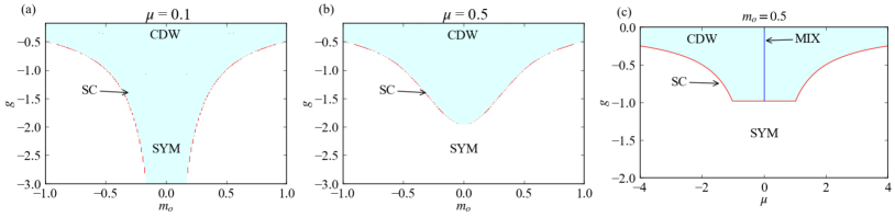
Figure S4: Phase diagrams in the $(g,\mu)$ and $(g,m_{o})$ planes for non-zero $m_{o}$ and $\mu$. (a) and (b) depict the $(g,m_{o})$ phase diagrams for $\mu=0.1$ and $\mu=0.5$, respectively. (c) illustrates the $(g,\mu)$ phase diagram for $m_{o}=0.5$. The phases represented by different colors in these diagrams are consistent with those in the main text.

S-I.5 Unveiling the Correlation: Initial Topological States and $(g_{1},g_{2})$ Interaction-Induced Phase Transitions

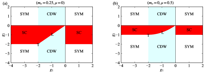
Figure S5: The ($g_{1}$,$g_{2}$)-phase portrait of the model, the white region labeled as SYM corresponds to the phase with unbroken symmetry, the red region labeled as SC represents the Superconducting phase, and the blue region labeled as CDW represents the charge-density-wave phase. The T point denotes the tricritical point, and the line labeled as L represents the phase boundary in the third quadrant. (a): The ($g_{1}$,$g_{2}$)-phase portrait at ($m_{o}=0.25,\mu=0$). (b): The ($g_{1}$,$g_{2}$)-phase portrait at ($m_{o}=0$ and $\mu=0.5$).

In this Section, we undertake a comprehensive analysis of the system’s phase diagram in the $(g_{1},g_{2})$ parameter space, we analyze the phase structure in the planes defined by the parameters ($g_{1},g_{2}$). Furthermore, we will investigate the relationship between the initial topological state of the system and the phase transitions induced by interactions. Remarkably, this specific aspect remains unexplored in the existing literature. We recognize that the topology of the Haldane model is determined by the Chern number: $C=\frac{1}{2}(\text{sgn}(\mu+m_{o})-\text{sgn}(\mu-m_{o}))$, which depends on the relative magnitude of the chemical potential and the Haldane mass term. Specifically, when $\mu>m_{o}$, $C=0$ and the system resides in a topologically trivial state; when $\mu<m_{o}$, $C=1$ and the system becomes a topological insulator. We first discuss two extreme scenarios: 1. $m_{o}\neq 0$, $\mu=0$; 2. $m_{o}=0$, $\mu\neq 0$. These cases correspond to two distinct topological states ($C=1$, $0$). Using Eq. (S-I.2), we derive the respective thermodynamic potentials (TDP) as follows:

$$V_{m_{o}}\equiv\Omega^{ren}(\Delta,\sigma,m_{o})=\frac{\sigma^{2}}{2\pi g_{1}}+\frac{\Delta^{2}}{2\pi g_{2}}+\frac{1}{12\pi}(|\Delta+m_{o}+\sigma|^{3}+|\Delta+m_{o}-\sigma|^{3}+|\Delta-m_{o}+\sigma|^{3}+|\Delta-m_{o}-\sigma|^{3}),$$ (S34)

$$V_{\mu}\equiv\Omega^{ren}(\Delta,\sigma,\mu)=\frac{\sigma^{2}}{2\pi g_{1}}+\frac{\Delta^{2}}{2\pi g_{2}}+\frac{1}{6\pi}(|\Delta+\sqrt{\mu^{2}+\sigma^{2}}|^{3}+|\Delta-\sqrt{\mu^{2}+\sigma^{2}}|^{3})\,.$$ (S35)

Solving the system of equations, $\begin{cases}\frac{\partial V_{i}}{\partial\Delta}=0,\\ \frac{\partial V_{i}}{\partial\sigma}=0.\end{cases}$($i=m_{o},\mu$), we analytically determine the system’s order parameters and the conditions for phase boundaries in these two extreme scenarios. The corresponding phase diagrams are depicted below:

Fig. S5 (a) presents the ($g_{1}$, $g_{2}$) phase diagram in the topological insulator state, where the analytically derived tricritical point T is located at $g_{1}=g_{2}=-\frac{1}{2|m_{o}|}$. The Superconducting order parameter $\Delta_{0}(m_{o})=\frac{-\frac{1}{g_{2}}+\sqrt{\frac{1}{g_{2}^{2}}-4m_{o}^{2}}}{2}$ and the CDW order parameter $\sigma_{0}(m_{o})=\frac{-\frac{1}{g_{1}}+\sqrt{\frac{1}{g_{1}^{2}}-4m_{o}^{2}}}{2}$. Fig. S5 (b) depicts the ($g_{1}$, $g_{2}$) phase diagram in the topologically trivial state, with the tricritical point T located at $g_{1}=-\frac{1}{|\mu|},g_{2}=-\frac{1}{2|\mu|}$. The Superconducting order parameter $\Delta_{0}(\mu)=\frac{-\frac{1}{g_{2}}+\sqrt{\frac{1}{g_{2}^{2}}-4\mu^{2}}}{2}$ and the CDW order parameter $\sigma_{0}(\mu)=\sqrt{\frac{1}{g_{1}^{2}}-\mu^{2}}$.

Upon comparing ($a$) and ($b$), it is evident that the expressions for the triple point T differ in these two extreme scenarios. This observation leads us to pose a question: Is the coordinate of the triple point T related to the topology of the system? Specifically, when the initial system is in a topological state, is the coordinate of T topologically protected? The answer is affirmative; the coordinate of the triple point T is indeed topologically protected. We have demonstrated this by numerically solving the phase diagram of the system when both $\mu$ and $m_{o}$ are simultaneously non-zero, thereby proving that the coordinate of the triple point T is topology-dependent. The numerical phase diagram is presented in Fig. S6 and S7.

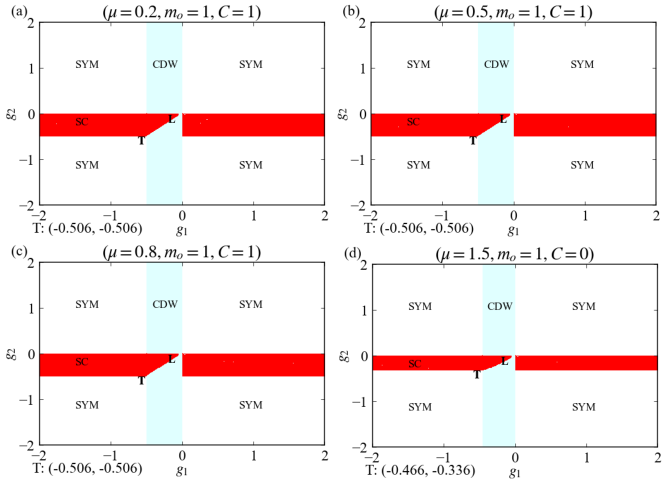
Figure S6: The ($g_{1},g_{2}$)-phase portrait for fixed chemical potential and Haldane mass term. The blue and red regions denote the CDW and SC phases, respectively. The tricritical point is marked as T, and the phase boundary L separates the two phases in the third quadrant. Figures (a), (b), and (c) depict the phase diagrams for the topological insulator state $(C=1)$, while Figure (d) illustrates the phase diagram for the topologically trivial state. Each diagram is generated by holding the magnitude of $m_{o}$ constant and progressively increasing the magnitude of $\mu$. The coordinates of the tricritical point T, computed numerically, are provided in the lower left corner of each figure.

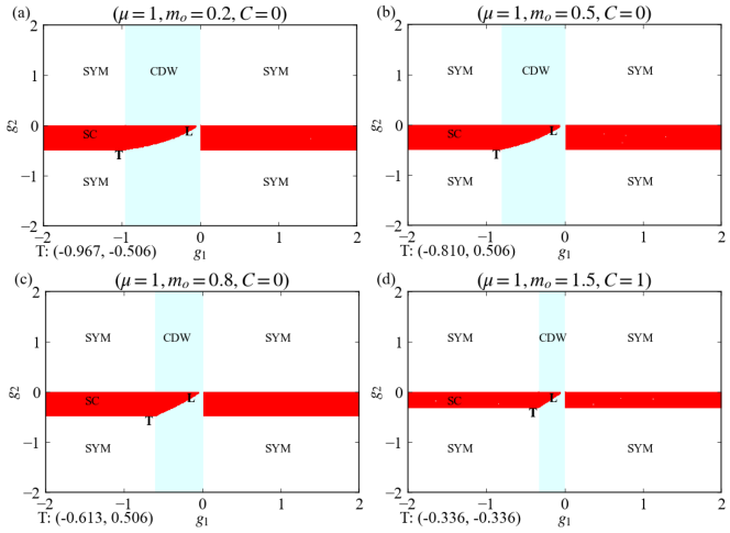
Figure S7: The ($g_{1},g_{2}$)-phase portrait for fixed chemical potential and Haldane mass term. Figures (a), (b), and (c) depict the phase diagrams for the topological trivial state $(C=0)$, while Figure (d) illustrates the phase diagram for the topologically insulator state. Each diagram is generated by holding the magnitude of $\mu$ constant and progressively increasing the magnitude of $m_{o}$.

When the system initially resides in a topological insulator state, i.e., $\mu<m_{o}$, the expression for the coordinates of the triple point in the $(g_{1},g_{2})$ plane remains constant at ($-\frac{1}{2|m_{o}|}$, $-\frac{1}{2|m_{o}|}$), irrespective of the value of the chemical potential $\mu$. Furthermore, the phase boundary L is a straight line.

Conversely, when the system initially resides in a topologically trivial state, i.e., $\mu>m_{o}$, the expression for the coordinates of the triple point in the $(g_{1},g_{2})$ plane becomes ($-\sqrt{\frac{1}{\mu^{2}+2m_{o}^{2}}}$,$-\frac{1}{2|\mu|}$), and the phase boundary L becomes a curve.

Therefore, the topology of the system not only protects the coordinates of the triple point T induced by interaction-induced phase transitions but also preserves the geometric shape of the phase boundary L. Our conclusions are summarized in the subsequent table.

Chern Number	$C=1$	$C=0$
Coordinates of T in the $(g_{1},g_{2})$ plane	$\left(-\frac{1}{2|m_{o}|},-\frac{1}{2|m_{o}|}\right)$	$\left(-\sqrt{\frac{1}{\mu^{2}+2m_{o}^{2}}},-\frac{1}{2|\mu|}\right)$
Geometry Of The Phase Boundary L	The Line $g_{2}=g_{1}$	Curve

S-I.6 Realization proposal using ultracold atoms

In a realistic experiment, we note that the realization of the Haldane-Hubbard model is already attainable in cold atoms, and it is possible now to study the quantum phase transitions discussed here. To be specific, we can use a polarized ultracold Fermi gas of ⁴⁰K atoms, here we choose the hyperfine state $|F,m_{F}\rangle=|9/2,-7/2\rangle$ by applying certain magnetic fields Tarruell et al. (2012); Jotzu et al. (2014), and tunable $p$-wave interactions have been well implemented utilizing this species of atom in experiments Regal et al. (2003); Günter et al. (2005); Ticknor et al. (2004). We load the atoms into the honeycomb optical lattice at a wavelength of $\lambda=826$ nm with potential $V(x,y)=-V_{x1}\sin^{2}(k_{L}x)-V_{x2}\cos^{2}(k_{L}x)-V_{y}\cos^{2}(k_{L}y)-2\sqrt{V_{x2}V_{y}}\cos(k_{x})\cos(k_{y})$. Here $V_{x1}=5.0E_{R},V_{x2}=0.46E_{R}$ are the lattice depths of two collinear beams along $x$ to create a standing wave, $V_{y}=2.2E_{R}$ is the lattice depth of the perpendicular beam along $y$ to create a spacing honeycomb lattice, and $k_{L}=2\pi/\lambda$. The recoil energy of such an optical lattice is $E_{R}=h^{2}/(2m\lambda^{2})\approx 7.26$kHz. The frequency detuning between the $x_{1}$ and $x_{2}$ beams should be set as $\pi$, whereas the same frequency for $x_{2}$ and $y$ beams, to control the energy offset $\mu$ between A-B sublattices. And the phase difference of beams along $x$ and $y$ can control the imaginary part of NNN hopping. Using a Wannier function calculation Uehlinger et al. (2013), we extract the amplitude of the NN hopping $t\approx 530$Hz, and the NNN hopping $t^{\prime}\approx 15$Hz.

Using the technique of $p$-wave Feshbach resonance, we can obtain Hubbard interaction $U$ as mentioned. The quantum phase transitions here are signaled by the several quasiparticle gaps, which would have dramatic effects on dynamic structure factor that can be measured by Bragg spectroscopy Vogels et al. (2002); Clément et al. (2009); Ernst et al. (2010). We expect that, the charge-density wave gap $\sigma$ and superconductor gap $\Delta$ can be distinguished by different characteristics by spectroscopy measurement.

References

Neto et al. (2009)A. C. Neto, F. Guinea,
N. M. Peres, K. S. Novoselov, and A. K. Geim, Reviews of Modern Physics 81, 109 (2009).
Haldane (1988)F. D. M. Haldane, Physical Review Letters 61, 2015 (1988).
Neupert et al. (2011)T. Neupert, L. Santos,
C. Chamon, and C. Mudry, Physical Review Letters 106, 236804 (2011).
Read and Green (2000)N. Read and D. Green, Physical Review
B 61, 10267 (2000).
Xu et al. (2011)G. Xu, H. Weng, Z. Wang, X. Dai, and Z. Fang, Physical Review Letters 107, 186806 (2011).
Yu et al. (2010)R. Yu, W. Zhang, H.-J. Zhang, S.-C. Zhang, X. Dai, and Z. Fang, Science 329, 61 (2010).
Thonhauser and Vanderbilt (2006)T. Thonhauser and D. Vanderbilt, Physical Review B 74, 235111 (2006).
Chang et al. (2013)C.-Z. Chang, J. Zhang,
X. Feng, J. Shen, Z. Zhang, M. Guo, K. Li, Y. Ou, P. Wei, L.-L. Wang, et al., Science 340, 167 (2013).
Herbut (2006)I. F. Herbut, Physical review letters 97, 146401 (2006).
Herbut et al. (2009)I. F. Herbut, V. Juričić, and B. Roy, Physical Review B 79, 085116 (2009).
Hickey et al. (2016)C. Hickey, L. Cincio,
Z. Papić, and A. Paramekanti, Physical Review
Letters 116, 137202
(2016).
Vanhala et al. (2016)T. I. Vanhala, T. Siro,
L. Liang, M. Troyer, A. Harju, and P. Törmä, Physical Review Letters 116, 225305 (2016).
Cangemi et al. (2019)L. Cangemi, A. Mishchenko,
N. Nagaosa, V. Cataudella, and G. De Filippis, Physical Review Letters 123, 046401 (2019).
Yi et al. (2021)T.-C. Yi, S. Hu, E. V. Castro, and R. Mondaini, Physical Review B 104, 195117 (2021).
Miao et al. (2019)J.-J. Miao, D.-H. Xu,
L. Zhang, and F.-C. Zhang, Physical Review B 99, 245154 (2019).
Mai et al. (2023)P. Mai, B. E. Feldman, and P. W. Phillips, Physical Review
Research 5, 013162
(2023).
Yanes et al. (2022)T. H. Yanes, M. Płodzień, M. M. Sinkevičienė, G. Žlabys, G. Juzeliūnas, and E. Witkowska, Physical Review Letters 129, 090403 (2022).
Castro et al. (2023)P. Castro, D. Shaffer,
Y.-M. Wu, and L. H. Santos, Physical Review Letters 131, 026601 (2023).
Herbut and Mandal (2023)I. F. Herbut and S. Mandal, arXiv
preprint arXiv:2305.17264 (2023).
Herbut (2023)I. F. Herbut, arXiv
preprint arXiv:2304.07654 (2023).
Palumbo and Pachos (2014)G. Palumbo and J. K. Pachos, Physical Review D 90, 027703 (2014).
Palumbo and Pachos (2013)G. Palumbo and J. K. Pachos, Physical Review Letters 110, 211603 (2013).
Cirio et al. (2014)M. Cirio, G. Palumbo, and J. K. Pachos, Physical Review
B 90, 085114 (2014).
Fernández et al. (2021)L. Fernández, V. S. Alves, M. Gomes,
L. O. Nascimento, and F. Peña, Physical Review D 103, 105016 (2021).
Fernández et al. (2020)L. Fernández, V. S. Alves, L. O. Nascimento, F. Peña, M. Gomes, and E. Marino, Physical Review
D 102, 016020 (2020).
Alves et al. (2017)V. S. Alves, R. O. Junior,
E. Marino, and L. O. Nascimento, Physical Review D 96, 034005 (2017).
Khunjua et al. (2017)T. Khunjua, K. Klimenko,
R. Zhokhov, and V. Zhukovsky, Physical Review D 95, 105010 (2017).
Khunjua et al. (2018)T. Khunjua, K. Klimenko, and R. Zhokhov, Physical Review
D 98, 054030 (2018).
Khunjua et al. (2019)T. Khunjua, K. Klimenko, and R. Zhokhov, Physical Review
D 100, 034009 (2019).
Ebert et al. (1994)D. Ebert, H. Reinhardt, and M. Volkov, Progress in
Particle and Nuclear Physics 33, 1 (1994).
Li et al. (2021)J. Li, G. Cao, and L. He, Physical Review D 104, 074026 (2021).
Ebert et al. (2001)D. Ebert, K. Klimenko, and H. Toki, Physical Review D 64, 014038 (2001).
Ebert et al. (2002)D. Ebert, V. Khudyakov,
V. C. Zhukovsky, and K. Klimenko, Physical Review D 65, 054024 (2002).
Ebert and Klimenko (2010)D. Ebert and K. Klimenko, Physical Review D 82, 025018 (2010).
Ebert et al. (2011)D. Ebert, N. Gubina,
K. Klimenko, S. Kurbanov, and V. C. Zhukovsky, Physical Review D 84, 025004 (2011).
Ebert et al. (2014)D. Ebert, T. Khunjua,
K. Klimenko, and V. C. Zhukovsky, Physical Review
D 90, 045021 (2014).
Ebert et al. (2015)D. Ebert, T. Khunjua,
K. Klimenko, and V. C. Zhukovsky, Physical Review
D 91, 105024 (2015).
Khunjua et al. (2022)T. Khunjua, K. Klimenko, and R. Zhokhov, Physical Review
D 106, 085002 (2022).
Gubaeva et al. (2022)M. Gubaeva, T. Khunjua,
K. Klimenko, and R. Zhokhov, Physical Review D 106, 125010 (2022).
Gies and Janssen (2010)H. Gies and L. Janssen, Physical Review
D 82, 085018 (2010).
Gomes et al. (1991)M. Gomes, R. Mendes,
R. Ribeiro, and A. da Silva, Physical Review D 43, 3516 (1991).
(43)See the Supplemental
Materials.
Ebert et al. (2016)D. Ebert, T. Khunjua,
K. Klimenko, and V. C. Zhukovsky, Physical Review
D 93, 105022 (2016).
Klimenko et al. (2012)K. Klimenko, R. Zhokhov, and V. C. Zhukovsky, Physical Review
D 86, 105010 (2012).
Gomes and Ramos (2021)Y. Gomes and R. O. Ramos, Physical Review B 104, 245111 (2021).
Gomes and Ramos (2023)Y. Gomes and R. O. Ramos, Physical Review B 107, 125120 (2023).
Carrington (2019)M. Carrington, Physical Review B 99, 115432 (2019).
Dudal et al. (2018)D. Dudal, A. J. Mizher, and P. Pais, Physical Review D 98, 065008 (2018).
Gusynin et al. (2007)V. Gusynin, S. Sharapov, and J. Carbotte, International
Journal of Modern Physics B 21, 4611 (2007).
Luo et al. (2015a)X. Luo, Y. Yu, and L. Liang, Physical Review B 91, 125126 (2015a).
Luo et al. (2015b)X. Luo, Y. Lan, Y. Yu, and L. Liang, Physical Review Letters 114, 249101 (2015b).
Muller-Kirsten and Wiedemann (2010)H. J. Muller-Kirsten and A. Wiedemann, Introduction to
Supersymmetry, Vol. 80 (World
Scientific Publishing Company, 2010).
Labelle (2010)P. Labelle, Supersymmetry
Demystified (McGraw Hill Professional, 2010).
Martin (2010)S. P. Martin, in Perspectives on
Supersymmetry II (World Scientific, 2010) pp. 1–153.
Sun et al. (2013)F. Sun, X.-L. Yu,
J. Ye, H. Fan, and W.-M. Liu, Scientific Reports 3, 2119 (2013).
Sun and Ye (2023a)F. Sun and J. Ye, arXiv preprint
arXiv:2303.06541 (2023a).
Sun and Ye (2023b)F. Sun and J. Ye, arXiv preprint
arXiv:2303.07251 (2023b).
Klipstein (2021)P. Klipstein, Physical Review B 104, 195407 (2021).
Chen et al. (2015)C.-Z. Chen, H. Liu, H. Jiang, Q.-f. Sun, Z. Wang, and X. Xie, Physical Review B 91, 214202 (2015).
Zhao et al. (2021)P.-L. Zhao, X.-B. Qiang,
H.-Z. Lu, and X. Xie, Physical Review Letters 127, 176601 (2021).
Li et al. (2020)C.-A. Li, B. Fu, Z.-A. Hu, J. Li, and S.-Q. Shen, Physical Review Letters 125, 166801 (2020).
Li et al. (2017)X. Li, Q. Niu, et al., Physical Review B 95, 241411 (2017).
Lee and Qi (2014)C. H. Lee and X.-L. Qi, Physical Review
B 90, 085103 (2014).
Zhang et al. (2014)G.-F. Zhang, Y. Li, and C. Wu, Physical Review B 90, 075114 (2014).
Yang et al. (2019)F. Yang, S.-J. Jiang, and F. Zhou, Physical Review B 100, 054508 (2019).
Peskin (2018)M. Peskin, An introduction to
quantum field theory (CRC press, 2018).
Srednicki (2007)M. Srednicki, Quantum field
theory (Cambridge University Press, 2007).
Tarruell et al. (2012)L. Tarruell, D. Greif,
T. Uehlinger, G. Jotzu, and T. Esslinger, Nature 483, 302 (2012).
Jotzu et al. (2014)G. Jotzu, M. Messer,
R. Desbuquois, M. Lebrat, T. Uehlinger, D. Greif, and T. Esslinger, Nature 515, 237 (2014).
Regal et al. (2003)C. A. Regal, C. Ticknor,
J. L. Bohn, and D. S. Jin, Phys. Rev. Lett. 90, 053201 (2003).
Günter et al. (2005)K. Günter, T. Stöferle, H. Moritz, M. Köhl, and T. Esslinger, Phys. Rev. Lett. 95, 230401 (2005).
Ticknor et al. (2004)C. Ticknor, C. A. Regal,
D. S. Jin, and J. L. Bohn, Phys. Rev. A 69, 042712 (2004).
Uehlinger et al. (2013)T. Uehlinger, G. Jotzu,
M. Messer, D. Greif, W. Hofstetter, U. Bissbort, and T. Esslinger, Phys. Rev. Lett. 111, 185307 (2013).
Vogels et al. (2002)J. M. Vogels, K. Xu, C. Raman, J. R. Abo-Shaeer, and W. Ketterle, Phys. Rev. Lett. 88, 060402 (2002).
Clément et al. (2009)D. Clément, N. Fabbri, L. Fallani, C. Fort, and M. Inguscio, Phys. Rev. Lett. 102, 155301 (2009).
Ernst et al. (2010)P. T. Ernst, S. Götze, J. S. Krauser, K. Pyka, D.-S. Lühmann, D. Pfannkuche, and K. Sengstock, Nat. Phys. 6, 56 (2010).