Electron heat flux and propagating fronts in plasma thermal quench via ambipolar transport

Abstract

The thermal collapse of a nearly collisionless plasma interacting with a cooling spot, in which the electron parallel heat flux plays an essential role, is investigated both theoretically and numerically. We show that such thermal collapse, which is known as thermal quench in tokamaks, comes about in the form of propagating fronts, originating from the cooling spot, along the magnetic field lines. The slow fronts, propagating with local ion sound speed, limit the aggressive cooling of plasma, which is accompanied by a plasma cooling flow toward the cooling spot. The extraordinary physics underlying such a cooling flow is that the fundamental constraint of ambipolar transport along the field line limits the spatial gradient of electron thermal conduction flux to the much weaker convective scaling, as opposed to the free-streaming scaling, so that a large electron temperature and hence pressure gradient can be sustained. The last ion front for a radiative cooling spot is a shock front where cold but flowing ions meet the hot ions.

I Introduction

When the magnetic field lines suddenly intercept solid surfaces that provide a sink for plasma energy and sometimes particles, a magnetized fusion-grade plasma can undergo a thermal collapse. This can happen, for example, in the thermal quench (TQ) of fusion plasma during either naturally occurring or intentionally triggered, mitigated tokamak disruptions. The naturally occurring tokamak disruption can be triggered when large-scale MHD activities turn nested flux surfaces into globally stochastic field lines that connect fusion-grade core plasma directly to the divertor/first wall Bondeson et al. (1991); Riccardo et al. (2002); Nardon et al. (2016); Sweeney et al. (2018). As a result, the substantial thermal energy of plasma is released within a few milliseconds Riccardo, Loarte, and JET EFDA Contributors (2005); Shimada et al. (2007); Nedospasov (2008), causing severe damage to the plasma facing components Loarte et al. (2007) (PFCs). Major disruptions are also intentionally triggered for disruption mitigation by injecting high-Z impurities, for example in the form of deliberately injected solid pellets Federici et al. (2003); Baylor et al. (2009); Combs et al. (2010); Paz-Soldan et al. (2020). The injected high-Z impurities into a pre-disruption plasma are intended to have the hot plasma deposit its thermal energy onto the pellet, so pellet materials can be ablated and ionized to be assimilated within the flux surface. The ablated pellet materials thus initially forms a radiative cooling mass (RCM) that provide strongly localized radiative cooling for the thermal energy of the surrounding fusion-grade plasma. The fact that the background plasma undergoes a thermal quench by transporting energy into the RCM, which through radiation can spread the heat load over the entire first wall, is the logic behind this approach for thermal quench mitigation. In both situations, the plasma will attach to an energy sink, being a vapor-shielded wall or the ablated pellet, and lose its energy via the fast parallel transport to the energy sink. It must be emphasized that for fusion-grade plasmas, which are nearly collisionless provided that the plasma mean-free-path, $\lambda_{mfp}\sim 10km$, is much longer than the magnetic connection length $L_{B}$ or the tokamak major radius, the TQ due to the presence of a cooling spot (energy sink) is in an exotic kinetic regime, in which the fast parallel transport along the field lines is expected to be the dominant mechanism. The normal expectation is that such nearly collisionless parallel transport of plasma thermal energy in the short magnetic connection length regime represents a worst-case scenario of a TQ in tokamaks, where the plasma thermal energy is released in the shortest possible time. Therefore, understanding the plasma TQ in such an exotic regime is critical for disruption mitigation.

For a nearly collisionless plasma, the prevailing view on the plasma TQ is that the electron thermal conduction flux along the magnetic field line $q_{e\parallel}$ plays the dominant role in the heat transport. Instead of following the Braginskii formula Braginskii (1965), $q_{e\parallel}$ in the collisionless limit is considered to be constrained by the free-streaming flux limiting Atzeni and Meyer-Ter-Vehn (2004)

$$q_{e\parallel}\approx\alpha_{e}n_{e}v_{th,e}T_{0},$$ (1)

where $\alpha_{e}$ is a numerical factor Bell (1985) $\sim 0.1$ and $v_{th,e}=\sqrt{T_{0}/m_{e}}$ the electron thermal speed with $T_{0}$ the surrounding plasma temperature. If the flux-limiting form is straightforwardly applied, such large $q_{e\parallel}$ will suggest a fast TQ occurring at the electron transit time $\tau_{tr}^{e}=L_{B}/v_{th,e}$. For a fusion-grade plasma with temperature $\sim 10keV$, we have $\tau_{tr}^{e}\sim 2.5\mu s\times(L_{B}/100m)$, which predicts remarkable fast TQ for $L_{B}<10^{4}m$. Such free-streaming form of thermal conduction is believed to dominate over the convective electron energy flux $\sim n_{e}V_{e\parallel}T_{e\parallel}$, since ambipolarity constrains $V_{e\parallel}\approx V_{i\parallel}\ll v_{th,e}$ and $V_{i\parallel}$ is bounded by the ion sound speed $c_{s}$.

However, it is worth noting that the inhibition of the electron thermal conduction in the nearly collisionless plasma has been extensively studied in astrophysics by considering the tangled magnetic fields Tribble (1989); Chandran and Cowley (1998) and plasma instabilities Jafelice (1992); Balbus and Reynolds (2008); Roberg-Clark et al. (2018) in order to reach the convection-dominated scenario of the thermal conduction, which would naturally yield the cooling flow that aggregates masses onto the cooling spot in clusters of galaxies Fabian (1994); Peterson and Fabian (2006); Aharonian et al. (2016); Zhuravleva et al. (2014). In a related vein for the fusion plasma, it is well known that the convective scaling of the electron thermal conduction is obtained at the entrance of the steady-state sheath, in which the plasma is nearly collisionless, as a result of the ambipolar transport Stangeby (2000, 1984); Tang and Guo (2016a). In this paper, we will show that the convective scaling with the parallel ion flow, in the electron thermal conduction itself or its spatial gradient, can be established throughout the bulk, quasineutral, and nearly collisionless plasma away from the wall due to ambipolar constraint. Such convective scaling comes about because the cooling of the surrounding plasma takes the form of propagating fronts that originate from the cooling spot and the fundamental ambipolar transport constraint between the slow fronts modifies the thermal conduction heat flux. As a result, a robust plasma cooling flow into the cooling spot will be developed due to the retained large electron temperature and hence pressure gradient Zhang, Li, and Tang (2023). Such weaker convective scaling of the electron thermal conduction, via itself or its gradient, is also critically important for a slower TQ of the fusion plasmas by modifying the core plasma cooling processes Li, Zhang, and Tang (2023). This should be contrasted with a straightforward application of the flux-limiting form for electron parallel thermal conduction, which would yield a much faster TQ on a time scale that is around a factor of $\sqrt{m_{i}/m_{e}}$ faster. Had one unwisely deployed the Braginskii parallel thermal conducivity instead for such a nearly collisionless plasma, an even faster TQ would be obtained in numerical simulations if the plasma has collisional mean-free-path longer than the system size.

Here we follow the previous Letter of Ref. Zhang, Li, and Tang, 2023 on the subject and present the details of numerical diagnostics, the analyses of the propagating fronts’ characteristics, and the underlying physics, as well as the electron thermal conduction flux. The first-principles fully kinetic simulations were performed with the VPIC Bowers et al. (2008) code to investigate the parallel transport physics in the TQ of a nearly collisionless plasma. A prototype one-dimensional slab model is considered with a normalized background magnetic field, where an initially uniform plasma with constant temperature $T_{0}\sim 10keV$ and density $n_{0}\sim 10^{19}m^{-3}$ is filled the whole domain. The plasma is signified as semi-infinite with the right simulation boundary simply reflecting the particles. We notice that such boundary condition would not affect the plasma dynamics as long as the later-defined electron fronts haven’t arrived there yet. This indicates that we consider $t<L_{B}/v_{th,e}$. However, for longer time scale, the basic physics holds, which affects the TQ processes Li, Zhang, and Tang (2023). A cooling spot is modeled at the left boundary as a thermobath that mimics a radiative cooling spot, which conserves particles by re-injecting electron-ion pairs (equal to the ions across the boundary) with a radiatively clamped temperature $T_{w}\ll T_{0}$. For comparison, an absorbing boundary, as a sink to both the particles and energy that absorbs all the particles hitting the left boundary, is also considered for simulations. We found that these two types of cooling spots show remarkable similarities in plasma cooling so the absorbing boundary is quite useful for understanding the underlying physics.

For both thermobath and absorbing boundary, the TQ is found to be governed by the formations of propagating fronts (e.g., see Fig. 1). Particularly, for the former (latter), there are four (three) fronts: the first two have speeds scale with the electron thermal speed $v_{th,e}$ and thus are named electron fronts, while the other two (one) propagate at speeds that scale with the local ion sound speed $c_{s}$ and thus named ion fronts. Based on the underlying physics and their roles in the TQ dynamics, these fronts can be named the precooling front (PF), precooling trailing front (PTF), recession front (RF), and cooling front (CF, for the thermobath boundary only), respectively, as illustrated in Fig. 1. The precooling and recession fronts describe the onset of $T_{\parallel}$ cooling of electrons and ions, respectively, which are independent of the cooling spot types. In contrast, the precooling trailing and cooling fronts will not only play a role in $T_{\parallel}$ cooling but also reflect the onset of $T_{\perp}$ cooling via the dilution with the cold recycled particles for the thermobath boundary. It should be noted that the propagating fronts for the rapid cooling of a nearly collisionless plasma, as described and reported here, are not the artifact of the boundary conditions deployed in the simulation. In a forthcoming paper that focuses on the impurity ion assimilation by a cooling plasma, the same front propagation physics are found in a plasma where a hot and dilute plasma cools against a cold and dense plasma, that is initially in pressure balance between the two regions.

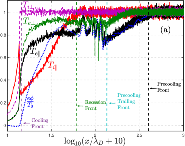
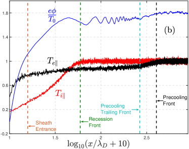
Figure 1: Normalized electron and ion temperature (by $T_{0}$), and electrostatic potential (by $T_{0}/e$) at $\omega_{pe}t=163$ for the thermobath boundary with $T_{w}=0.01T_{0}$ (a) and the absorbing boundary (b) from the first-principles kinetic simulations of collisionless plasma (similar results are obtained for nearly collisionless plasma with $\lambda_{mfp}\gg L_{B}$). Notice that the perpendicular temperature for the absorbing boundary are nearly unperturbed and hence ignored. The sheath entrance here is denoted as where the plasma parameters remain quasi-steady. We should emphasize that the electrostatic potential is directly integrated from the instantaneous electric field that contains large amplitude Langmuir waves, which thus is only used as a guide for the qualitative behavior of the quiescent ambipolar potential.

The rest of the paper is organized as follows. In section II we elucidate the underlying physics of electron fronts, while the ion front(s) physics are investigated in section III. The electron thermal conduction flux within the recession layer (the region between the recession and cooling front for the thermobath boundary or between the recession front and sheath entrance for the absorbing boundary), which is essential for the formation of the plasma cooling flow, will be discussed in section IV. We will conclude in section V.

II Electron fronts

We first investigate the physics underlying the electron fronts. In a nearly collisionless plasma, the cooling of the parallel electron temperature $T_{e\parallel}$ is mainly due to the cutoff of electron distribution function as a result of the loss of high energy electrons that overcome the electrostatic potential barrier, i.e., $v_{\parallel}>v_{c}$ where $v_{c}=\sqrt{2e\Delta\Phi/m_{e}}$ with $\Delta\Phi=\Phi(x)-\Phi_{\rm min}$, $\Phi(x)$ being the local electrostatic potential and $\Phi_{\rm min}$ the minimum potential. For the absorbing boundary, $\Phi_{\rm min}$ is the boundary potential, while for the thermobath boundary, $\Phi_{\rm min}$ is the local minimum potential just behind the cooling front as shown in Fig. 1. It must be highlighted that, for the thermobath boundary, the same ambipolar field can accelerate some cold recycled electrons towards the upstream to form an electron beam with velocity $V_{b}\approx v_{c}$ due to the energy gain at the ambipolar potential, e.g., see Fig. 2, the front of which is between the electron fronts that will be discussed later in this section. As a result, the electron distribution can be approximated as

$$f_{e}(v_{\parallel},v_{\perp})=\frac{n_{m}\left(\Phi(x)\right)}{\sqrt{2\pi}v_{th,e}^{3}}e^{-\left(v_{\parallel}^{2}+v_{\perp}^{2}\right)/2v_{th,e}^{2}}\Theta\left(1-\frac{v_{\parallel}}{v_{c}}\right)+\frac{n_{b}}{2\pi v_{\perp}}\delta(v_{\perp})\delta(v_{\parallel}-v_{c}),$$ (2)

where $\Theta(x)$ is the Heaviside step function that vanishes for $x<0$ and $\delta(x)$ the Dirac delta function, $n_{m}$ is the plasma density associated with the cutoff Maxwellian (the original surrounding electrons) and $n_{b}$ the recycled (cold) electron beam density. For the absorbing boundary (or ahead of the cold electron beam front for the thermobath boundary), $n_{b}=0$, for which one obtains

$$n_{e}= \frac{1+\textup{Erf}(v_{c}/\sqrt{2}v_{th,e})}{2}n_{m}+n_{b},$$ (3)

$$n_{e}V_{e\parallel}= -\frac{n_{m}v_{th,e}}{\sqrt{2\pi}}e^{-v_{c}^{2}/2v_{th,e}^{2}}+n_{b}v_{c},$$ (4)

$$n_{e}T_{e\parallel}= n_{m}T_{0}\left[\frac{1+\textup{Erf}(v_{c}/\sqrt{2}v_{th,e})}{2}-\frac{v_{c}}{\sqrt{2\pi}v_{th,e}}e^{-{v_{c}^{2}}/{2v_{th,e}^{2}}}\right]+n_{b}T_{0}\frac{v_{c}^{2}}{v_{th,e}^{2}}-n_{e}T_{0}\frac{V_{e\parallel}^{2}}{v_{th,e}^{2}},$$ (5)

$$q_{en}= -\frac{n_{m}v_{th,e}T_{0}}{\sqrt{2\pi}}\left(\frac{v_{c}^{2}}{v_{th,e}^{2}}+2\right)e^{-v_{c}^{2}/2v_{th,e}^{2}}+n_{b}T_{0}v_{c}\frac{v_{c}^{2}}{v_{th,e}^{2}}-3n_{e}T_{e\parallel}V_{e\parallel}-n_{e}m_{e}V_{e\parallel}^{3}.$$ (6)

Here $n_{e}=\int f_{e}d^{3}\mathbf{v}$ is the electron density, $V_{e\parallel}=\int v_{\parallel}f_{e}d^{3}\mathbf{v}/n_{e}$ the parallel electron flow, $T_{e\parallel}=\int m_{e}\tilde{v}_{\parallel}^{2}f_{e}d^{3}\mathbf{v}/n_{e}$ the parallel electron temperature, and $q_{en}=\int m_{e}\tilde{v}_{\parallel}^{3}f_{e}d^{3}\mathbf{v}$ the parallel thermal conduction flux of the parallel degree of freedom Chew et al. (1956), where $\tilde{v}_{\parallel}\equiv(v_{\parallel}-V_{e\parallel})$.

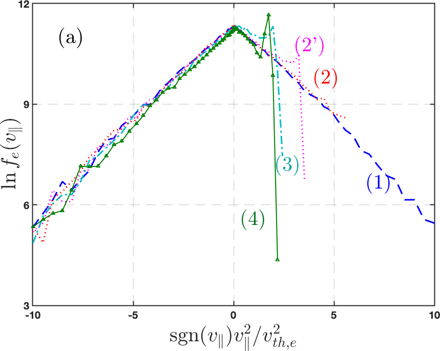
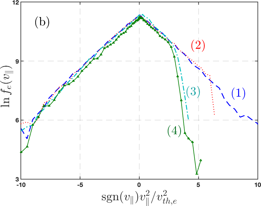
Figure 2: Electron distributions at different locations from VPIC simulations corresponding to Fig. 1. (a) is for the thermobath boundary and (b) is for the absorbing boundary. These distributions are chose from: (1) ahead of the precooling front, (2) between the precooling and precooling trailing fronts (for the thermobath boundary, it is ahead of the cold electron beam front where $T_{e\perp}$ is unperturbed), (3) between the recession and precooling trailing fronts and (4) within the recession layer. For the thermobath boundary, ($2^{\prime}$) is behind the cold electron beam front but ahead of the precooling trailing front.

The ambipolar transport constraint implies $V_{e\parallel}\approx V_{i\parallel}$, one immediate result of which is that the last terms in $T_{e\parallel}$ and $q_{en}$ that are proportional to $V_{e\parallel}^{2,3}$ are negligible as $V_{e\parallel}\approx V_{i\parallel}\tilde{<}v_{th,i}\ll v_{c}\sim v_{th,e}$ with $v_{th,i}=\sqrt{T_{0}/m_{i}}$. This is especially so between the electron fronts where the plasma flow is nearly unperturbed since it is controlled by the ion fronts. Without the plasma flow ahead of the ion fronts, the plasma energy equation shows that the collapse of $T_{e\parallel}$ is mainly driven by the conduction heat flux $q_{en}$

$$n_{e}\left(\frac{\partial}{\partial t}T_{e\parallel}+V_{e\parallel}\frac{\partial}{\partial x}T_{e\parallel}\right)+2n_{e}T_{e\parallel}\frac{\partial}{\partial x}V_{e\parallel}+\frac{\partial}{\partial x}q_{en}=0.$$ (7)

Between the electron fronts, the fraction of electron beam for the thermobath boundary is small $n_{b}\ll n_{m}$ (notice that $n_{b}=0$ for the absorbing boundary). Thus, the ambipolar transport constraint $V_{e\parallel}\approx V_{i\parallel}$ requires $v_{c}>\sqrt{2}v_{th,e}$ as seen from Eq. (4) and Fig. 2. Such a condition gurantees that

$$\frac{dq_{en}}{dx}\approx n_{e}v_{c}\frac{\partial T_{e\parallel}}{\partial x}.$$ (8)

As a result, the energy equation in Eq. (7) has the solution $T_{e\parallel}=T_{e\parallel}(x-v_{c}t)$ for $n_{e}\approx n_{0}$, revealing that $v_{c}$ is the recession speed of $T_{e\parallel}$ or the velocity space void in $f_{e}(v_{\parallel})$ propagates upstream with a speed of $v_{c}$. It must be emphasized that the electron fronts are fast $\sim v_{th,e}$ but only produce a modest amount of $T_{e\parallel}$ cooling as seen from Eq. (5) for $v_{c}\gg v_{th,e}$, which results from the ambipolar transport constraint. Moreover, Eq. (6) illustrates that the electron parallel conduction flux does scale as the free-streaming limit, $q_{en}\propto n_{e}v_{th,e}T_{0}$ but with a small coefficient as a function of $v_{c}(\Phi)$.

Now we can define the electron fronts and provide their propagating speeds by using the local $v_{c}$. The precooling front (PF) is used to denote the onset of $T_{e\parallel}$ cooling, which can be defined as where $T_{e\parallel}(v_{c})$ has a detectable cooling. It is independent of the boundary condition since it is ahead of the recycled electron beam front. Considering the VPIC noise, we choose the speed of the PF as

$$U_{PF}=2.4v_{th,e},$$ (9)

for which $T_{e\parallel}(v_{c}=U_{PF})\approx 0.95T_{0}$ as seen from Eq. (5) with $n_{b}=0$. It agrees well with the simulation results in Fig. 3. While the precooling trailing front (PTF) comes about because the ambipolar potential and hence the plasma cooling mainly varies behind the recession front (e.g., see Fig. 1) due to the limit of the plasma flow. Therefore, there must be a smallest cutoff velocity $v_{c}^{\rm min}=\sqrt{2e(\Delta\Phi)_{\rm RF}/m_{e}}\sim v_{th,e}$ ahead of the recession front (RF) determined by the reflecting potential, $(\Delta\Phi)_{\rm RF}=\Phi_{\rm RF}-\Phi_{\rm min}$ with $\Phi_{\rm RF}$ the potential at the RF. Such $v_{c}^{\rm min}$ will define the PTF speed

$$U_{PTF}=v_{c}^{\rm min}=\sqrt{2e(\Delta\Phi)_{\rm RF}/m_{e}}.$$ (10)

The fact that the cutoff velocity between the PTF and RF satisfies $v_{c}\approx v_{c}^{\rm min}$ demonstrates that the PTF will leave a nearly constant $T_{e\parallel}=T_{e\parallel}(U_{PTF})$ behind. For an absorbing boundary with $n_{b}=0$, from Eq. (5) we obtain

$$T_{e\parallel}(U_{PTF})\approx T_{0}\left[1-\sqrt{{e\left(\Delta\Phi\right)_{\rm RF}}/{\pi T_{0}}}e^{-{e\left(\Delta\Phi\right)_{\rm RF}}/{T_{0}}}\right].$$ (11)

For the thermobath boundary, the aforementioned cold electron beam, which are accelerated by the electrostatic potential all the way to $\sim U_{PTF}$, will reduce $T_{e\parallel}(U_{PTF})$. This is because such electron beam will reduce the reflecting potential for the thermobath boundary compared to that for the absorbing boundary as shown in Fig. 1 (this will be studied in section IV), which results in a slower PTF (smaller $U_{PTF}$) and hence deeper cooling of $T_{e\parallel}$ than those for the absorbing boundary.

Interestingly, the faster PTF for the absorbing boundary nearly coincides with the $T_{e\perp}$ collapse front (cold recycled electron beam front) for the thermobath boundary as shown in Fig. 1. This is because, at the beginning of the thermal collapse, the number of recycled electrons is not high enough to cause an appreciable reduction of the reflecting potential compared to that for the absorbing boundary. Such nearly equalized reflecting potential $(\Delta\Phi)_{\rm RF}$ will accelerate the recycled electrons, which dilutely cool $T_{e\perp}$, to $U_{PTF}$ for the absorbing boundary case. A fitting speed of $1.4v_{th,e}$ for $T_{e\perp}$ precooling front is shown in Fig. 3.

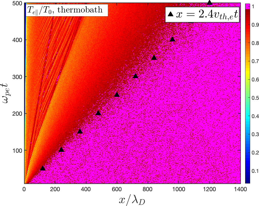
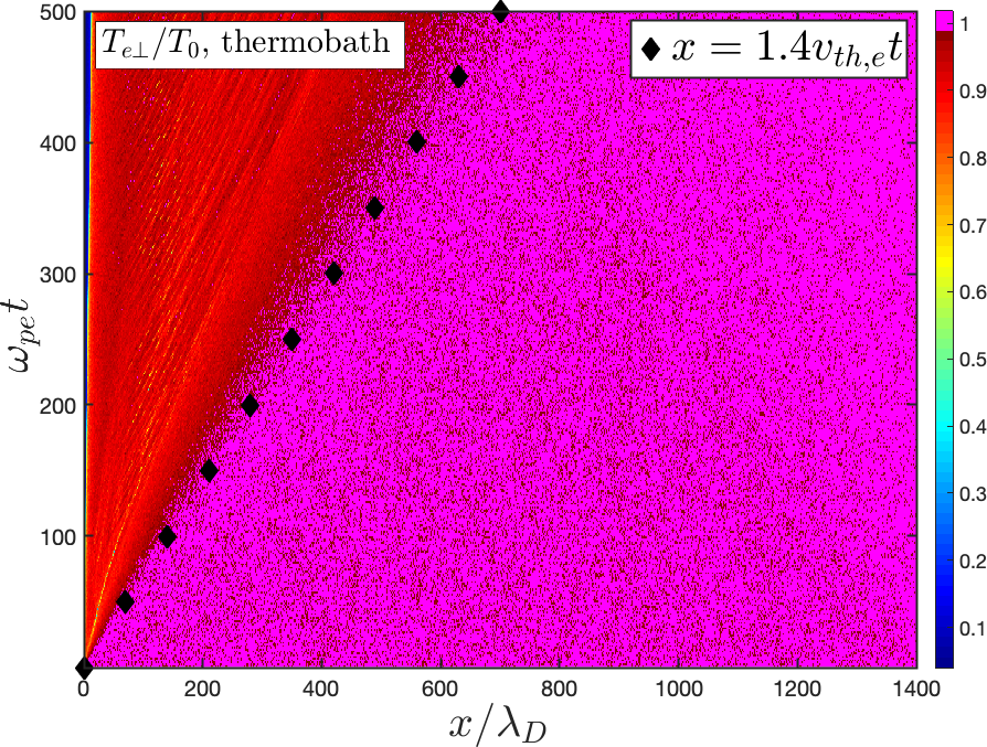
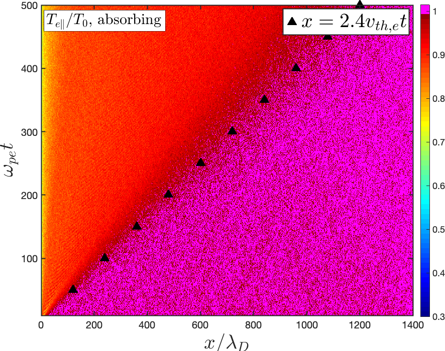
Figure 3: Contour plots of normalized electron temperature and the corresponding fitting precooling front (black triangles) for the same simulations in Fig. 1, where the left boundary conditions are labeled. For the thermobath boundary, we also plot the fitting front of $T_{e\perp}$ collapse (black diamonds). The nearly unperturbed values are colored as magenta.

III Ion fronts

The ion front(s) not only describes the plasma temperature cooling but also controls the plasma density evolution and the associated cooling flow generation. This section is dedicated to studying the underlying physics of the ion front(s), taking into account that the plasma thermal conduction is forced to be convective, in the form of either itself or its gradient, due to the ambipolar transport, which will be investigated in the next section. As a result, the electron pressure gradient remains large to drive plasma flow towards the cooling spot, which is known in astrophysics as the cooling flow. Fabian (1994); Peterson and Fabian (2006); Aharonian et al. (2016); Zhuravleva et al. (2014)

We first highlight that the cooling front (CF) for the thermobath boundary case is the front of cold recycled ions. Therefore, the plasma ahead the CF is free of cold recycled ions. Such a block of cold ions by the CF is complete and thus different from that of the cold recycled electrons discussed above, where some of them can cross the CF and penetrate into the upstream plasma as cold recycled electron beams. As a result, we can examine the recession front (RF) and the recession layer between the RF and CF by ignoring the recycled ions. In physics terms, the recession layer is a rarefaction wave in the nearly collisionless plasma, which is different from the rarefaction wave formed in a cold plasma interacting with a solid surface Allen and Andrews (1970); Cipolla and Silevitch (1981); Breizman and Kiramov (2021) considering the large plasma temperature and pressure gradients and the nature of the plasma heat fluxes. But the common feature of the rarefaction wave is that the plasma parameters recede steadily with local speed $\sim c_{s}$ and thus we can seek self-similar solutions of $n_{e,i},V_{e,i\parallel},T_{e,i\parallel}$ as functions of the self-similar variable $\xi\equiv x/t\sim c_{s}$ from the minimum model for an anisotropic plasma Chew et al. (1956); Chodura and Pohl (1971); Guo and Tang (2012)

$$\frac{\partial}{\partial t}n_{i}+\frac{\partial}{\partial x}\left(n_{i}V_{i\parallel}\right)=0,$$ (12)

$$m_{i}n_{i}\left(\frac{\partial}{\partial t}V_{i\parallel}+V_{i\parallel}\frac{\partial}{\partial x}V_{i\parallel}\right)+\frac{\partial}{\partial x}(p_{i\parallel}+p_{e\parallel})=0,$$ (13)

$$n_{i}\left(\frac{\partial}{\partial t}T_{i\parallel}+V_{i\parallel}\frac{\partial}{\partial x}T_{i\parallel}\right)+2n_{i}T_{i\parallel}\frac{\partial}{\partial x}V_{i\parallel}+\frac{\partial}{\partial x}q_{in}=0.$$ (14)

The force balance of electrons $en_{e}E_{\parallel}\approx-\partial p_{e\parallel}/\partial x$ and the quasi-neutral condition $n_{e}=Zn_{i}$ are used with $Z$ being the ion charge number, and $p_{e,i\parallel}=n_{e,i}T_{e,i\parallel}$. Notice that the quasi-neutrality ensures $V_{e\parallel}\approx V_{i\parallel}\ll v_{th,e}$ in the absence of net current and thus the force balance of electrons is valid within the recession layer due to the small inertia of electrons.

To complete these equations, we need closures for the parallel ion thermal conduction of the parallel degree of freedom $q_{in}\equiv\int m_{i}\left(\mathbf{v}_{\parallel}-V_{i\parallel}\right)^{3}f_{i}d\mathbf{v}$ and the electron pressure gradient. Within the recession layer, the ion distribution can be approximated by one-sided cutoff Maxwellian with a proper shift like in the presheath region Tang and Guo (2016a) and thus we can employ $q_{in}=\sigma_{i}T_{i\parallel}\Gamma_{i\parallel}$ with $\sigma_{i}\sim 1$ the energy transmission coefficient and $\Gamma_{i}=n_{i}V_{i\parallel}$. The spatial gradient of $q_{en}$ is shown to retain the convective energy transport scaling $\sim n_{e}V_{e\parallel}T_{e\parallel}$ over the recession layer (see the next section) so that we can approximate $\partial q_{en}/\partial x\approx\sigma_{e}\partial(n_{e}T_{e\parallel}V_{i\parallel})/\partial x$, where $\sigma_{e}\sim 1$ is analogous to $\sigma_{i}$. As a result, from the continuity and energy equations for ions in Eqs. (12, 14) and electrons, which have the same form as Eqs. (12, 14) but with $e$ replacing $i$ in the subscripts, we obtain

$$\frac{-\xi+(1+\sigma_{e,i})V_{e,i\parallel}}{3+\sigma_{e,i}}\frac{d\textup{ln}p_{e,i\parallel}}{d\xi}=\frac{d\textup{ln}V_{e,i\parallel}}{d\xi}.$$ (15)

Recalling the quasi-neutral condition $V_{e\parallel}\approx V_{i\parallel}$, one finds

$$\frac{d\textup{ln}p_{e\parallel}}{d\xi}\approx\mu\frac{d\textup{ln}p_{i\parallel}}{d\xi},$$ (16)

where $\mu=(3+\sigma_{e})/(3+\sigma_{i})\times[-\xi+(1+\sigma_{i})V_{i\parallel}]/[-\xi+(1+\sigma_{e})V_{i\parallel}]\sim 1$. In physics terms, Eq. (16) demonstrates an universal length scale for $p_{e,i\parallel}$ within the recession layer since the convective transport scaling dominates the thermal collapse of $T_{e,i\parallel}$. As a result, Eqs. (12-14) form a complete set of equations in the form of

$$\textbf{A}\left(\frac{dn_{i}}{d\xi},\frac{dV_{i\parallel}}{d\xi},\frac{dT_{i\parallel}}{d\xi}\right)^{T}=0,$$ (17)

where A is a matrix of $n_{i}$, $V_{i\parallel}$ and $T_{e,i\parallel}$. The non-trivial solution requires $det(\textbf{A})=0$, yielding

$$G =-\xi^{3}+\left(3+\sigma_{i}\right)V_{i\parallel}\xi^{2}-[\left(3+2\sigma_{i}\right)V_{i\parallel}^{2}-\left(1+\sigma_{i}/3\right)c_{s}^{2}]\xi$$

$$+\left(1+\sigma_{i}\right)V_{i\parallel}^{3}-\left(1+\sigma_{i}/3\right)c_{s}^{2}V_{i\parallel}=0,$$ (18)

where $c_{s}=\sqrt{3(\mu ZT_{e\parallel}+T_{i\parallel})/m_{i}}$ is approximated to the local ion sound speed. A uniquely monotonic solution of $\xi$ can be found in the recession layer as

$$\xi=[\sigma_{i}^{2}V_{i\parallel}^{2}/4+(1+\sigma_{i}/3)c_{s}^{2}]^{1/2}+(1+\sigma_{i}/2)V_{i\parallel},$$ (19)

by ignoring the explicit dependence on $\xi$ of $\mu$ in $c_{s}$. It shows that the recession speed $\xi$ is determined by the local ion flow and sound speed, and thus the recession layer is independent of the boundary condition (e.g., see Fig. 4). This is not surprising since the cold ions are blocked by the CF, while the recycled electron beam only moderately modifies the electron profiles ahead of the CF.

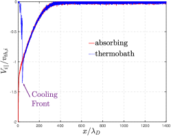
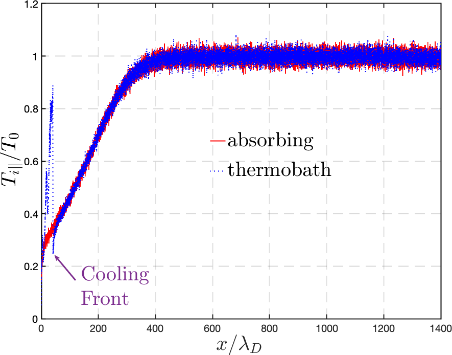
Figure 4: Profile of normalized ion density, parallel flow and temperature at $\omega_{pe}t=1357$ for the simulations in Fig. 1. The location of the cooling front is marked, ahead of which the ion state variables are aligned with each other for the different boundary conditions.

Let’s first use the self-similar solution of Eq. (19) to recover a known constraint on the plasma exit flow at an absorbing boundary where a non-neutral sheath would form next to it. The sheath entrance can not propagate further upstream in this case so $\xi=0$. Thus Eq. (19) predicts an ion exit flow speed of

$$V_{i\parallel}=-\sqrt{\frac{1+\sigma_{i}/3}{1+\sigma_{i}}}c_{s}\equiv-\sqrt{(\beta 3ZT_{e\parallel}+3T_{i\parallel})/m_{i}},$$ (20)

with

$$\beta=\frac{1-\frac{1}{Ze\Gamma_{i}}\frac{\partial q_{in}}{\partial\phi}}{1+\frac{1}{e\Gamma_{e}}\frac{\partial q_{en}}{\partial\phi}},$$ (21)

and $\Gamma_{e,i}=n_{e,i}V_{e,i\parallel}$. This is consistent with the Bohm criterion for plasma in steady state ($d/dt=0$) when including the heat flux in the transport model Tang and Guo (2016b); Li et al. (2022a, b). More importantly, Eq. (19) predicts the speed of the RF, which is defined as $V_{i\parallel}=0$

$$U_{RF}=\xi(V_{i\parallel}=0)=\sqrt{(1+\sigma_{i}/3)}c_{s}.$$ (22)

Recalling Eqs. (12-14), such definition of the RF also denotes the onset of $n_{i}$ and $T_{i\parallel}$ drop. Moreover, since the electron temperature is only moderately reduced at the RF, $T_{e\parallel}\approx T_{e\parallel}(U_{PTF})$, we have $U_{RF}\approx 2.8v_{th,i}$ for $Z=1$ and $\mu=1$ from Eq. (22). This is consistent with the VPIC simulations as shown in Fig. 5.

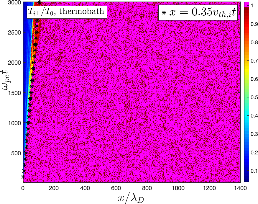
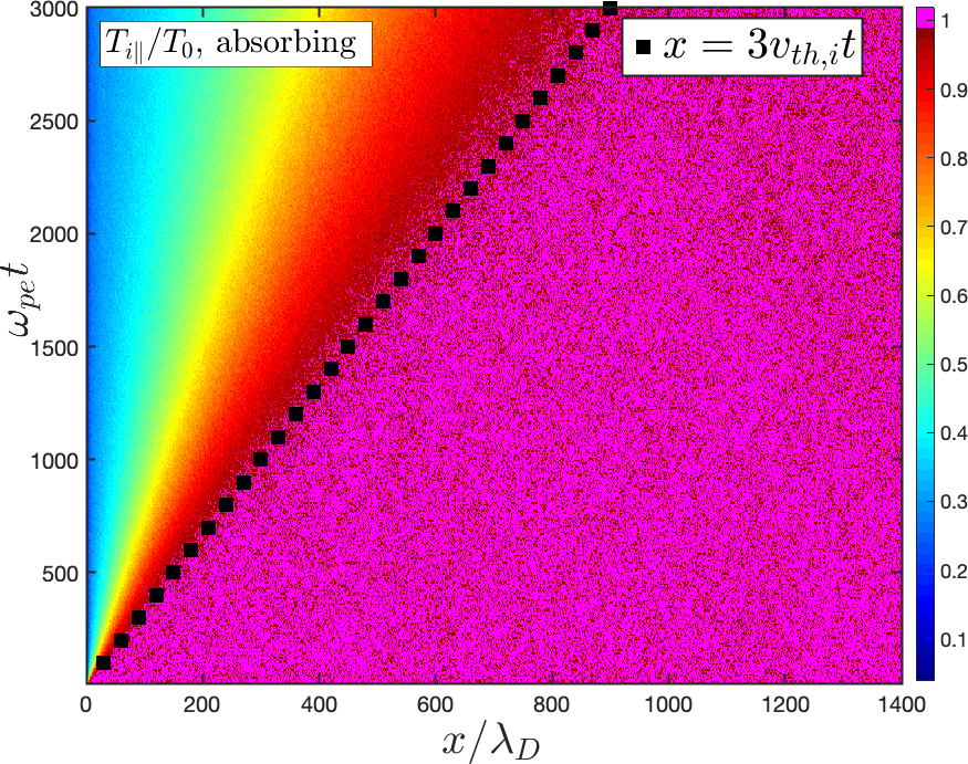
Figure 5: Contour plots of normalized ion temperature and the corresponding fitting recession front (black squares) for the same simulations in Fig. 1, where the left boundary conditions are labeled. For the thermobath boundary case, we also plot the fitting cooling front (black stars), which denotes the onset of $T_{i\perp}$ collapse. The nearly unperturbed values are colored as magenta.

The cooling front (CF) in the thermobath boundary case is where the hot ions meet the cold ions as illustrated in Fig. 6. In fact, it is a shock front, across which all the plasma state variables have jumps as shown in Figs. 1-5. Particularly, the ions undergo heating in the parallel direction when the plasma flow runs into the CF, where the substantial ion flow energy in the recession layer is converted into ion thermal energy as shown in Figs. 1, 4, and 5. Such conversion is via the mixing of the cooling flow ions with the cold recycled ions (e.g., see Fig. 6), the latter of which are accelerated from the boundary to the CF by the inverse pressure gradient due to the pressure pile up at the boundary. As a result, these cold recycled ions will offset the plasma flow generated by the surrounding ions as shown in Fig. 4. In sharp contrast to ions, the electrons will undergo cooling via dilution with high-density cold electrons so $T_{e\parallel}\sim T_{w}$ behind the CF as shown in Figs. 1 and 3. Moreover, the presence of the CF and the associated cooling zone behind the CF is of fundamental importance to $T_{i\perp}$ and $T_{e\perp}$ cooling via dilution and thus the CF represents a deep cooling of electrons.

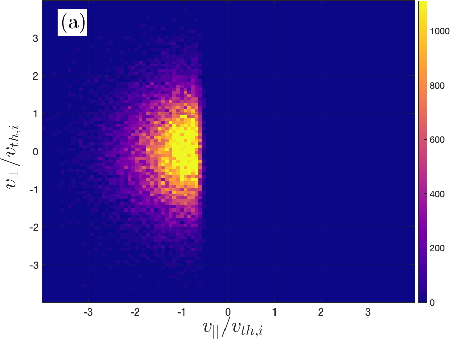
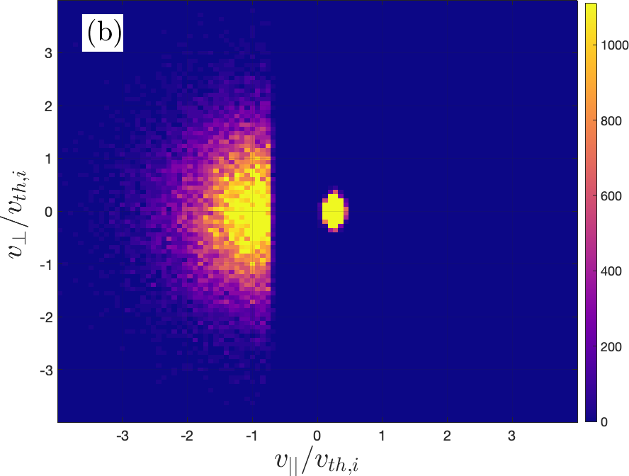
Figure 6: Ion distribution just ahead (a) and behind (b) the cooling front for the thermobath boundary case corresponding to Fig. 1. Here $v_{\parallel}$ is the velocity in the parallel direction, while $v_{\perp}$ is the velocity in one of the perpendicular directions. Behind the cooling front, there are two components in the ion distribution, which have quite different perpendicular temperature, indicative of the cooling flow ions from the upstream and cold recycled ions from the boundary.

To find the speed of the shock (cooling) front, we can match the conserved quantities across the front while simply ignoring the thermal conduction flux due to the convective scaling of its gradient. In the moving frame of reference with the shock front, we have

$$n_{i1}\tilde{V}_{i\parallel 1}=n_{i2}\tilde{V}_{i\parallel 2},$$ (23)

$$m_{i}n_{i1}\tilde{V}_{i\parallel 1}^{2}+(T_{i\parallel 1}+ZT_{e\parallel 1})n_{i1}=m_{i}n_{i2}\tilde{V}_{i\parallel 2}^{2}+(T_{i\parallel 2}+ZT_{e\parallel 2})n_{i2},$$ (24)

$$m_{i}n_{i1}\tilde{V}_{i\parallel 1}^{3}+3(T_{i\parallel 1}+ZT_{e\parallel 1})n_{i1}\tilde{V}_{i\parallel 1}=m_{i}n_{i2}\tilde{V}_{i\parallel 2}^{3}+3(T_{i\parallel 2}+ZT_{e\parallel 2})n_{i2}\tilde{V}_{i\parallel},$$ (25)

where the subscripts $1$ and $2$ denote, respectively, the ion variables behind (downstream) and ahead (upstream) of the shock front, and $\tilde{V}_{i\parallel}=V_{i\parallel}-U_{CF}$ with $U_{CF}$ being the CF speed. As a result, we find

$$\frac{\tilde{V}_{i\parallel 1}}{\tilde{V}_{i\parallel 2}}=\frac{\tilde{V}_{i\parallel 2}^{2}+3(ZT_{e\parallel 2}+T_{i\parallel 2})/m_{i}}{2\tilde{V}_{i\parallel 2}^{2}}\equiv\frac{1+1/M_{2}^{2}}{2}.$$ (26)

In the upstream (recession layer), we have shown that $-V_{i\parallel}+\xi=c_{s}=\sqrt{3(ZT_{e\parallel}+T_{i\parallel})/m_{i}}$ as seen from Eq. (19) with $\sigma_{i}=0$. Therefore, the Mach number $M_{2}=|V_{i\parallel}-U_{CF}|/c_{s}$ is near unity and thus the CF is a low Mach number shock. It should be noted that, near the CF, the ion flow is further accelerated by the large ambipolar field compared to that for the absorbing boundary (e.g., see Fig. 4), increasing $M_{2}$ slightly above the unity. These conditions ensure the stable flow upstream and downstream of the shock Kuznetsov and Osin (2018). Further simplification to obtain the CF speed will be $|V_{i\parallel 1}|\ll U_{CF}$ due to the offset of plasma velocity by the cold recycled particles as shown in Fig. 4 so that

$$U_{CF}\approx-\tilde{V}_{i\parallel 2}\approx c_{s,2},$$ (27)

with $M_{2}\approx 1$. This indicates that the CF propagates with the upstream ion sound speed. Since the plasma temperature at the CF is considerably lower than that at the RF, we have $U_{CF}<U_{RF}.$

IV Electron thermal conduction flux under the ambipolar transport constraint

In this section, we investigate the electron thermal conduction flux within the recession layer under the ambipolar transport constraint $V_{e\parallel}\approx V_{i\parallel}$. Both model analyses and first-principle simulations using VPIC will be provided.

IV.1 Analytical results

For the electron distribution in Eq. (2), the electron density, parallel flow, temperature, and thermal conduction heat flux are given in Eqs. (3-6), from which one finds an expression for $T_{e\parallel}$ and $q_{en}$

$$T_{e\parallel}= T_{0}\left[1-\frac{n_{b}}{n_{e}}+\frac{V_{e\parallel}v_{c}}{v_{th,e}^{2}}-\frac{V_{e\parallel}^{2}}{v_{th,e}^{2}}\right],$$ (28)

$$q_{en}= -2n_{b}v_{c}T_{0}+\left(\frac{v_{c}^{2}}{v_{th,e}^{2}}+2\right)n_{e}V_{e\parallel}T_{0}-3n_{e}T_{e\parallel}V_{e\parallel}-n_{e}m_{e}V_{e\parallel}^{3}.$$ (29)

Then from Eqs. (4, 28, 29), we see that the impact of the cold beam can be ignored in the limit of a small cold beam component

$$n_{b}v_{c}<n_{e}V_{e\parallel}.$$ (30)

Since $v_{c}\sim v_{th,e},$ one has in this limit

$$\frac{n_{b}}{n_{e}}<\sqrt{\frac{m_{e}}{m_{i}}},$$ (31)

under which we cover the absorbing boundary case with $n_{b}=0$. Otherwise, the cold beam can make a big difference.

For an absorbing boundary or a small beam component, the ambipolar transport will limit the cutoff velocity to be large $v_{c}\propto v_{th,e}\sqrt{2\ln(v_{th,e}/V_{i\parallel})},$ so that $V_{e\parallel}\approx V_{i\parallel}$ as seen from Eq. (4). However, in the large cold beam component limit,

$$n_{b}v_{c}\sim n_{b}v_{th,e}\gg n_{e}V_{e\parallel},$$ (32)

or equivalently, $n_{b}/n_{e}\gg\sqrt{m_{e}/m_{i}}$, one must have, to the leading order in $\sqrt{m_{e}/m_{i}},$

$$n_{b}v_{c}\approx\frac{n_{m}v_{th,e}}{\sqrt{2\pi}}e^{-v_{c}^{2}/2v_{th,e}^{2}},$$ (33)

which means that the cold beam and the truncated Maxwellian both carry significant electron particle fluxes, but nearly cancel each other to produce a much slower electron flow $V_{e\parallel}$ that matches onto $V_{i\parallel}$ for ambipolar transport. Compared to the small beam component limit, the requirement for large $v_{c}$ and hence $\Delta\Phi$ in the absorbing boundary case is relaxed due to the large electron beam component. Therefore, the reflecting potential and hence $U_{PTF}$ for the thermobath boundary is smaller than those for the absorbing boundary as discussed in section II. From Eqs. (3, 33), we obtain

$$\frac{n_{b}}{n_{e}}=\frac{1}{1+\sqrt{\frac{\pi}{2}}\left[1+\textup{Erf}(v_{c}/\sqrt{2}v_{th,e})\right]\frac{v_{c}}{v_{th,e}}e^{v_{c}^{2}/2v_{th,e}^{2}}}.$$ (34)

One can easily verify that $n_{b}/n_{e}$ is a monotonically decreasing function of $v_{c}$. It is important to note that $v_{c}$ can not vanish (or $n_{b}=n_{e}$), otherwise, $T_{e\parallel}$ would become negative as seen from Eq. (28). However, $v_{c}$ can become very small and so does $T_{e\parallel}$, indicating that the plasma temperature can drop to the value set by the temperature of the beam-like cold plasma at the CF.

The necessary constraint to sustain the large gradient of $T_{e\parallel}$ within the recession layer to drive the plasma flow towards the cooling spot is on the spatial gradient of $q_{en}$, which can be argued in the following. Assuming the recession layer span a length of $L_{R}$, from Eq. (7), the convective energy transport terms (the term that is proportional to $V_{e\parallel}$ itself or its gradient) follow the scaling of $n_{e}T_{e\parallel}V_{e\parallel}/L_{R}.$ Therefore, a necessary condition for forming the recession layer by keeping a large $T_{e\parallel}$ gradient will require

$$\frac{\partial q_{en}}{\partial x}\lesssim\frac{n_{e}T_{e\parallel}V_{e\parallel}}{L_{R}}.$$ (35)

This is indeed the case due to the ambipolar transport constraint. To see it, we re-write $q_{en}$ in Eq. (29) as

$$q_{en}\approx-\alpha_{e}n_{e}v_{th,e}T_{0}+\sigma_{e}n_{e}V_{e\parallel}T_{e\parallel},$$ (36)

where

$$\alpha_{e} \equiv 2\frac{n_{b}}{n_{e}}\frac{v_{c}}{v_{th,e}},$$ (37)

$$\sigma_{e} \equiv\left(\frac{v_{c}^{2}}{v_{th,e}^{2}}+2\right)\frac{T_{0}}{T_{e\parallel}}-3.$$ (38)

The second term carries over from the absorbing boundary case where no cold electron beam component is present, while the first term is entirely due to the presence of a cold beam component, as it is proportional to $n_{b}/n_{e}$. This first term is of great importance since it covers the conventional electron free-streaming scaling of $q_{en}$, although the coefficient critically depends on the fractional density of the cold beam component.

In the case of an absorbing boundary, $n_{b}/n_{e}=0,$ we have

$$q_{en}\approx\sigma_{e}n_{e}V_{e\parallel}T_{e\parallel},$$ (39)

which illustrates that the parallel electron heat flux itself scales as the convective energy transport scaling. While in the large cold beam limit, the first term of $q_{en}$ dominates

$$q_{en}\approx-\alpha_{e}n_{e}v_{th,e}T_{0},$$ (40)

for $v_{c}>V_{e\parallel}$ so that $q_{en}$ itself has electron mass scaling $m_{e}^{-1/2}$, recovering the free-streaming limit. However, its spatial gradient over the recession layer retains the convective transport scaling. This is because the cold beam continuity equation in the collisionless recession layer has

$$n_{b}v_{c}\approx const.,$$ (41)

to obtain which we have ignored $\partial n_{b}/\partial t$ in the beam continuity equation because if we seek the self-similar solution between the ion fronts, we have $\partial n_{b}/\partial t\approx-\xi\partial n_{b}/\partial x\ll v_{c}\partial n_{b}/\partial x$ with $\xi\sim c_{s}\ll v_{c}\sim v_{th,e}$. This indicates that $\partial(n_{b}v_{c})/\partial x=-\partial n_{b}/\partial t\sim c_{s}n_{b}/L_{R}$ contributes less to $\partial q_{en}/\partial x$ than that from the second term in Eq. (36) since $n_{b}<n_{e}$. Therefore, we have reached the interesting point that the electron parallel heat flux is primarily carried by the electron beam to follow the free electron streaming scaling, but remarkably, its spatial gradient is given by the convective energy transport scaling.

IV.2 First-principles kinetic simulations

The first-principles kinetic simulations have confirmed all the above analytical results. Specifically, to check the convective transport scaling of $q_{en}$, i.e., $q_{en}\propto m_{i}^{-1/2}$, we have conducted simulations by employing different ion-electron mass ratios, i.e., $m_{i}/m_{e}=100,~{}400,~{}900$ and $1600$. Eq. (19) indicates that both the ion flow and local recession speed $\xi$ in the recession layer scales with $m_{i}^{-1/2}$. Therefore, to overlap the recession layer to the same location for different $m_{i}$, we should choose temporal moments with constant $\omega_{pi}t$ for different cases. Here $\omega_{pi}$ is the ion plasma frequency.

In Fig. 7 we plot the profiles of $q_{en}$ for the absorbing boundary case, which demonstrates that $q_{en}$ itself indeed follows the convective transport scaling $q_{en}\propto V_{i\parallel}$ within the recession layer, although the coefficient $\sigma_{e}$ slightly increases with $m_{i}$. Such variation of $\sigma_{e}$ comes from the weakly positive dependence of $v_{c}$ on $m_{i}$ via $v_{c}\sim v_{th,e}\sqrt{2\ln(v_{th,e}/V_{i\parallel})}$.

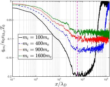
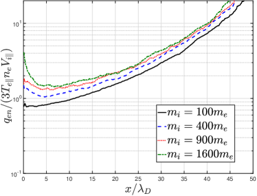
Figure 7: Profiles of $q_{en}$ at $\omega_{pi}t=20.3$ for different $m_{i}/m_{e}$ with the absorbing boundary. Left: $q_{en}$, normalized by the initial quantities $n_{0}T_{0}v_{th,e}$, at the whole domain, where the recession front at $x\approx 60\lambda_{D}$ is labeled by the vertical dashed line; Right: $q_{en}$, normalized by the convection heat flux $3n_{e}V_{i\parallel}T_{e\parallel}$, behind the recession front (away from the recession front where $V_{i\parallel}\approx 0$).

For the case of a thermobath boundary, Fig. 8 shows that $q_{en}$ is nearly independent of $m_{i}$ and instead recovers a flux-limiting form for the heat conduction flux with $\alpha_{e}\sim 0.2$ in the recession layer. But its gradient within the recession layer still has the convective transport scaling, i.e., $<dq_{en}/dx>\propto m_{i}^{-1/2}$. As discussed in Eq. (36), the free-streaming form is recovered for $q_{en}$ because of the dominating cold beam contribution of $-2n_{b}v_{c}T_{0}.$ This cold beam term, however, doesn’t contribute to $<dq_{en}/dx>$ since the cold beam flux $n_{b}v_{c}$ in the collisionless recession layer is constant as shown in Eq. (41). To quantify the beam contribution to the electron heat flux as well as the particle flux, we have separated the cold recycled electrons from the original electrons. In Fig. 9, we show the contributions to the electron particle flux $n_{e}V_{e\parallel}$ from both recycled $n_{b}v_{c}$ and the original trapped electrons $n_{m}V_{m\parallel}\equiv n_{e}V_{e\parallel}-n_{b}v_{c}$ for the $m_{i}=100m_{e}$ case. It shows that both the recycled and the original trapped electrons carry significant electron particle flux but nearly cancel each other to generate much smaller $n_{e}V_{e\parallel}\ll n_{b}v_{c}$. Notice that $n_{b}v_{c}$ has the electron scaling $n_{b}v_{c}\propto v_{th,e}$ while $n_{e}V_{e\parallel}$ has the ion scaling $n_{e}V_{e\parallel}\propto v_{th,i}$ so that the difference between them is even stronger for larger $m_{i}$. Fig. 9 also confirms that $n_{b}v_{c}$ is nearly constant within the recession layer as expected, so it doesn’t contribute to $dq_{en}/dx$. It is worth noting that the cold electron front is ahead of the PTF. Ahead of the PTF, $n_{b}v_{c}$ varies in space so that $q_{en}$ itself and its gradient continuously follow the free-streaming scaling.

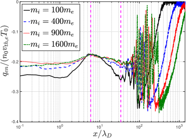
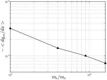
Figure 8: Profiles of $q_{en}$ (left) and its averaged gradient $<dq_{en}/dx>$ (right) in the recession layer at $\omega_{pi}t=13.6$ for the thermobath boundary with $T_{w}=0.01$. The averaged region in the recession layer is labeled by vertical dashed lines.

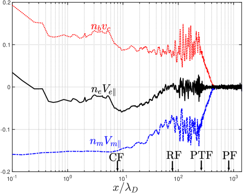
Figure 9: $n_{e}V_{e\parallel}$, $n_{b}v_{c}$ and $n_{m}V_{m\parallel}\equiv n_{e}V_{e\parallel}-n_{b}v_{c}$, in the unit of $n_{0}v_{th,e}$, at $\omega_{pe}t=271$ for the thermobath boundary with $m_{i}/m_{e}=100$ and $T_{w}=0.01$. The locations for the four fronts are labeled.

V Conclusions

In conclusion, the thermal collapse of a nearly collisionless plasma interacting with a cooling spot is investigated both theoretically and numerically. For both types of cooling spots that signify, respectively, the radiative cooling masses (thermobath boundary) and a perfect particle and energy sink (absorbing boundary), we found that the thermal quench comes about in the form of propagating fronts that originate from the cooling spot. Particularly, for the thermobath boundary, two fast electron fronts have speeds that scale with the electron thermal speed $v_{th,e}$, and two slow ion fronts propagates at local ion sound speed $c_{s}$. The former denotes the fast but moderate cooling of electrons, while the latter represents the slow but aggressive cooling of electrons and ions.

The underlying physics behind these propagating fronts have been investigated, in which the electron thermal conduction heat flux $q_{en}$ is found to play an essential role. Specifically, the electron fronts are completely driven by $q_{en},$ which follows the free-streaming form ($q_{en}\propto n_{e}v_{th,e}T_{e\parallel}$). Such large thermal conduction flux is reminiscent of a very limited amount of $T_{e\parallel}$ drop over a very large volume. In contrast, the ion fronts are formed as a result of the full transport physics, the crucial one of which is the ambipolar transport constraint. Due to such ambipolar transport constraint, $q_{en}$ in the recession layer itself follows the convective energy transport scaling with the parallel plasma flow $V_{i\parallel}$ for the absorbing boundary. While for the thermobath boundary, the cold electron beam will restore the free-streaming limit of $q_{en}\sim-2n_{b}v_{c}T_{0}\propto v_{th,e}$, but its spatial gradient will follow the convective transport scaling since the beam particle flux ($n_{b}v_{c}$) remains nearly constant within the recession layer. As a result, the electron temperature and hence the pressure retains large spatial gradient to drive the plasma flow toward the cooling spot.

For a thermobath boundary that provides an energy sink while re-supplying cold particles, the plasma cooling flow eventually terminates against the cooling spot via a plasma shock, which we named the cooling front since it signifies the deep cooling of electrons to the radiatively clamped temperature $T_{w}$. It is shown that such a shock front will convert the ion flow energy into the ion thermal energy via the mixing of hot and cold ions behind the front, which completely blocks the cold ions from migrating upstream. Therefore, the cooling front and the associated cooling zone behind the cooling front are of fundamental importance to $T_{i\perp}$ and $T_{e\perp}$ cooling via dilution. Unlike the recycled cold ions, part of the recycled electrons can penetrate through the cooling front to reach the electron fronts, causing further cooling of the electrons behind the electron fronts.

References

- Bondeson et al. (1991) A. Bondeson, R. Parker, M. Hugon, and P. Smeulders, “MHD modelling of density limit disruptions in tokamaks,” Nuclear Fusion 31, 1695 (1991).
- Riccardo et al. (2002) V. Riccardo, P. Andrew, L. Ingesson, and G. Maddaluno, “Disruption heat loads on the JET MkIIGB divertor,” Plasma Physics and Controlled Fusion 44, 905 (2002).
- Nardon et al. (2016) E. Nardon, A. Fil, M. Hoelzl, G. Huijsmans, and JET contributors, “Progress in understanding disruptions triggered by massive gas injection via 3D non-linear MHD modelling with JOREK,” Plasma Physics and Controlled Fusion 59, 014006 (2016).
- Sweeney et al. (2018) R. Sweeney, W. Choi, M. Austin, M. Brookman, V. Izzo, M. Knolker, R. La Haye, A. Leonard, E. Strait, F. Volpe, et al., “Relationship between locked modes and thermal quenches in DIII-D,” Nuclear Fusion 58, 056022 (2018).
- Riccardo, Loarte, and JET EFDA Contributors (2005) V. Riccardo, A. Loarte, and JET EFDA Contributors, “Timescale and magnitude of plasma thermal energy loss before and during disruptions in JET,” Nuclear fusion 45, 1427 (2005).
- Shimada et al. (2007) M. Shimada, D. Campbell, V. Mukhovatov, M. Fujiwara, N. Kirneva, K. Lackner, M. Nagami, V. Pustovitov, N. Uckan, J. Wesley, et al., “Chapter 1: Overview and summary,” Nuclear Fusion 47, S1–S17 (2007).
- Nedospasov (2008) A. Nedospasov, “Thermal quench in tokamaks,” Nuclear fusion 48, 032002 (2008).
- Loarte et al. (2007) A. Loarte, B. Lipschultz, A. Kukushkin, G. Matthews, P. Stangeby, N. Asakura, G. Counsell, G. Federici, A. Kallenbach, K. Krieger, et al., “Power and particle control,” Nuclear Fusion 47, S203 (2007).
- Federici et al. (2003) G. Federici, P. Andrew, P. Barabaschi, J. Brooks, R. Doerner, A. Geier, A. Herrmann, G. Janeschitz, K. Krieger, A. Kukushkin, et al., “Key ITER plasma edge and plasma–material interaction issues,” Journal of Nuclear Materials 313, 11–22 (2003).
- Baylor et al. (2009) L. R. Baylor, S. K. Combs, C. R. Foust, T. C. Jernigan, S. Meitner, P. Parks, J. B. Caughman, D. Fehling, S. Maruyama, A. Qualls, et al., “Pellet fuelling, ELM pacing and disruption mitigation technology development for ITER,” Nuclear Fusion 49, 085013 (2009).
- Combs et al. (2010) S. K. Combs, S. J. Meitner, L. R. Baylor, J. B. Caughman, N. Commaux, D. T. Fehling, C. R. Foust, T. C. Jernigan, J. M. McGill, P. B. Parks, et al., “Alternative techniques for injecting massive quantities of gas for plasma-disruption mitigation,” IEEE transactions on plasma science 38, 400–405 (2010).
- Paz-Soldan et al. (2020) C. Paz-Soldan, P. Aleynikov, E. Hollmann, A. Lvovskiy, I. Bykov, X. Du, N. Eidietis, and D. Shiraki, “Runaway electron seed formation at reactor-relevant temperature,” Nuclear Fusion 60, 056020 (2020).
- Braginskii (1965) S. I. Braginskii, Reviews of Plasma Physics, ed. M. A. Leontovich, Vol.I, pp. 205-311 (Consultants Bureau, New York, 1965).
- Atzeni and Meyer-Ter-Vehn (2004) S. Atzeni and J. Meyer-Ter-Vehn, The physics of inertial fusion (Oxford University Press, Inc., 2004).
- Bell (1985) A. R. Bell, “Non-spitzer heat flow in a steadily ablating laser-produced plasma,” The Physics of Fluids 28, 2007–2014 (1985), https://aip.scitation.org/doi/pdf/10.1063/1.865378 .
- Tribble (1989) P. C. Tribble, “The reduction of thermal conductivity by magnetic fields in clusters of galaxies,” MNRAS 238, 1247–1260 (1989).
- Chandran and Cowley (1998) B. D. G. Chandran and S. C. Cowley, “Thermal conduction in a tangled magnetic field,” Phys. Rev. Lett. 80, 3077–3080 (1998).
- Jafelice (1992) L. C. Jafelice, “Plasma Wave Modes in Cooling Flows in Clusters of Galaxies,” The Astronomical Journal 104, 1279 (1992).
- Balbus and Reynolds (2008) S. A. Balbus and C. S. Reynolds, “Regulation of Thermal Conductivity in Hot Galaxy Clusters by MHD Turbulence,” Ap. J. 681, L65 (2008), arXiv:0806.0940 [astro-ph] .
- Roberg-Clark et al. (2018) G. T. Roberg-Clark, J. F. Drake, C. S. Reynolds, and M. Swisdak, “Suppression of electron thermal conduction by whistler turbulence in a sustained thermal gradient,” Phys. Rev. Lett. 120, 035101 (2018).
- Fabian (1994) A. C. Fabian, “Cooling flows in clusters of galaxies,” Annual Review of Astronomy and Astrophysics 32, 277–318 (1994), https://doi.org/10.1146/annurev.aa.32.090194.001425 .
- Peterson and Fabian (2006) J. Peterson and A. Fabian, “X-ray spectroscopy of cooling clusters,” Physics Reports 427, 1–39 (2006).
- Aharonian et al. (2016) F. Aharonian, H. Akamatsu, F. Akimoto, S. W. Allen, N. Anabuki, L. Angelini, K. Arnaud, M. Audard, H. Awaki, M. Axelsson, et al., “The quiescent intracluster medium in the core of the perseus cluster,” Nature 535, 117–121 (2016).
- Zhuravleva et al. (2014) I. Zhuravleva, E. Churazov, A. A. Schekochihin, S. W. Allen, P. Arévalo, A. C. Fabian, W. R. Forman, J. S. Sanders, A. Simionescu, R. Sunyaev, et al., “Turbulent heating in galaxy clusters brightest in x-rays,” Nature 515, 85–87 (2014).
- Stangeby (2000) P. C. Stangeby, The plasma boundary of magnetic fusion devices, Vol. 224 (Institute of Physics Pub. Philadelphia, Pennsylvania, 2000).
- Stangeby (1984) P. Stangeby, “Plasma sheath transmission factors for tokamak edge plasmas,” The Physics of fluids 27, 682–690 (1984).
- Tang and Guo (2016a) X.-Z. Tang and Z. Guo, “Kinetic model for the collisionless sheath of a collisional plasma,” Physics of Plasmas 23, 083503 (2016a).
- Zhang, Li, and Tang (2023) Y. Zhang, J. Li, and X.-Z. Tang, “Cooling flow regime of a plasma thermal quench,” Europhysics Letters 141, 54002 (2023).
- Li, Zhang, and Tang (2023) J. Li, Y. Zhang, and X.-Z. Tang, “Staged cooling of a fusion-grade plasma in a tokamak thermal quench,” Nuclear Fusion 63, 066030 (2023).
- Bowers et al. (2008) K. J. Bowers, B. Albright, L. Yin, B. Bergen, and T. Kwan, “Ultrahigh performance three-dimensional electromagnetic relativistic kinetic plasma simulation,” Physics of Plasmas 15, 055703 (2008).
- Chew et al. (1956) G. F. Chew, M. L. Goldberger, F. E. Low, and S. Chandrasekhar, “The boltzmann equation an d the one-fluid hydromagnetic equations in the absence of particle collisions,” Proceedings of the Royal Society of London. Series A. Mathematical and Physical Sciences 236, 112–118 (1956).
- Allen and Andrews (1970) J. Allen and J. Andrews, “A note on ion rarefaction waves,” Journal of Plasma Physics 4, 187–194 (1970).
- Cipolla and Silevitch (1981) J. Cipolla and M. Silevitch, “On the temporal development of a plasma sheath,” Journal of Plasma Physics 25, 373–389 (1981).
- Breizman and Kiramov (2021) B. N. Breizman and D. I. Kiramov, “Plasma sheath and presheath development near a partially reflective surface,” Journal of Plasma Physics 87 (2021).
- Chodura and Pohl (1971) R. Chodura and F. Pohl, “Hydrodynamic equations for anisotropic plasmas in magnetic fields. II. transport equations including collisions,” Plasma Physics 13, 645–658 (1971).
- Guo and Tang (2012) Z. Guo and X.-Z. Tang, “Parallel transport of long mean-free-path plasmas along open magnetic field lines: Plasma profile variation,” Physics of Plasmas 19, 082310 (2012), http://dx.doi.org/10.1063/1.4747167.
- Tang and Guo (2016b) X.-Z. Tang and Z. Guo, “Critical role of electron heat flux on bohm criterion,” Physics of Plasmas 23, 120701 (2016b).
- Li et al. (2022a) Y. Li, B. Srinivasan, Y. Zhang, and X.-Z. Tang, “Bohm criterion of plasma sheaths away from asymptotic limits,” Phys. Rev. Lett. 128, 085002 (2022a).
- Li et al. (2022b) Y. Li, B. Srinivasan, Y. Zhang, and X.-Z. Tang, “Transport physics dependence of bohm speed in presheath–sheath transition,” Physics of Plasmas 29, 113509 (2022b).
- Kuznetsov and Osin (2018) V. Kuznetsov and A. Osin, “On the parallel shock waves in collisionless plasma with heat fluxes,” Physics Letters A 382, 2052–2054 (2018).