Election Manipulation in Social Networks with Single-Peaked Agents

Abstract

Several elections run in the last years have been characterized by attempts to manipulate the result of the election through the diffusion of fake or malicious news over social networks. This problem has been recognized as a critical issue for the robustness of our democracy. Analyzing and understanding how such manipulations may occur is crucial to the design of effective countermeasures to these practices.

Many studies have observed that, in general, to design an optimal manipulation is usually a computationally hard task. Nevertheless, literature on bribery in voting and election manipulation has frequently observed that most hardness results melt down when one focuses on the setting of (nearly) single-peaked agents, i.e., when each voter has a preferred candidate (usually, the one closer to her own belief) and preferences of remaining candidates are inversely proportional to the distance between the candidate position and the voter’s belief. Unfortunately, no such analysis has been done for election manipulations run in social networks.

In this work, we try to close this gap: specifically, we consider a setting for election manipulation that naturally raises (nearly) single-peaked preferences, and we evaluate the complexity of election manipulation problem in this setting: while most of the hardness and approximation results still hold, we will show that single-peaked preferences allow to design simple, efficient and effective heuristics for election manipulation.

1 Introduction

Nowadays, online social networks have become a ubiquitous, fast, easily accessible source of information: e.g., Matsa and Shearer [32] showed that about one-fifth of American adults consults social media to read news. Interestingly a significant part of the interviewed people declared that social media news somehow altered their opinion [32]. This makes social networks a powerful tool that can be exploited to manipulate people’s minds about a particular theme, spreading targeted news to specific users. Indeed, this spread of information has been apparently exploited in many recent elections [2, 26, 18, 27]. The most prominent example has been the 2016 U.S. election: in the campaign preceding this event, fake news spreading has been so relevant that some commentators argued that the election’s outcome could be different if the campaign had been fair [2].

The relevance of the topic leads the AI community to investigate about the problem of manipulating elections by spreading information over social networks. Specifically, the problem has been modelled as follows: let $G=(V,E)$ be a graph representing the (online) social network of the voters, with $V$ being the set of voters and $E$ being the set of (possibly directed) social relationships between voters. Each voter $v\in V$ has a political opinion that somehow implies particular preferences over the set $C$ of candidates that, in turn, imply a particular vote according to the voting rule that controls the election. The manipulator has a (possibly unlimited) budget $B$ to spend to hire some voters, bribe them, and make them act as influencers to spread some news in favour of or against a target candidate $c^{*}\in C$. As a result of such influence, some voters (depending on their influenceability and the effectiveness of the hired influencers) will update their opinions and change their votes in favour of or against the target candidate. The aim of the manipulator is to choose the best set of influencers (not violating the budget constraint) to optimize a specific objective function that encodes the chances of victory of the target candidate $c^{*}$. Wilder and Vorobeychik [36] have been the first to deal with this problem. They indeed prove that it is hard to compute both the set of influencers that maximizes the probability of victory of $c^{*}$, and the one that optimizes the expected difference between the number of votes of $c^{*}$ and the number of votes of the best candidate different from $c^{*}$. However, for the latter problem there is a greedy algorithm that computes a constant approximation of the optimum [36]. These results have been extended to more complex settings, focusing, e.g., on different models of information diffusion, different voting rules, and different messages to spread [20, 1, 19].

These works complement the large literature in AI and social choice about bribery in elections [11, 12, 13, 23]: they focus on ways of altering the outcome of an election by changing the preference of a few of voters. Anyway, all these works do not take into account the possibility that manipulators could use voters’ social relationships to spread the manipulation. Most of the results in these works imply that it is computationally hard to compute the best way to alter an election. Still, most of these hardness results have been showed to melt down when the preferences of voters satisfy the realistic hypothesis of being single-peaked or nearly single-peaked [34, 25, 15, 24], where single-peakedness implies that candidates can be seen as ordered (e.g., along the political spectrum), voters have a preferred candidate (e.g., the one that is closer to their own political belief) and the preference towards remaining candidates decreases as the distance between their position and the one of the preferred candidate increases.

Our contribution.

Election manipulation involving information spreading in social networks has not been explicitly studied for the setting in which preferences are single-peaked. In this work we address this issue, by studying the problem of election manipulation through social influence in single-peaked scenarios. Specifically, we will build over known models of election manipulation in order to embed into them the principles of single-peakedness. Namely, in our model, each voter has an opinion on the topic of the voting and their ranking of alternatives depends on the distance between the candidates’ positions and the voter’s belief. Here, the diffusion of information has the effect to change the opinion of the voter, and hence it may alter her ranking, but still guaranteeing it to be single-peaked. This model can be also easily extended to encompass nearly single-peaked preferences: these, indeed, may simply arise from voters having a noisy view of candidates position. Given this model, the problem is to find, subject to a budget constraint, the set of “seeds” from which to start the information campaign that maximizes the margin of victory of the desired candidate.

It is not hard to check that previous hardness results extend also to this setting. Moreover, we show that there exists an approximation algorithm for the problem guaranteeing to return a set of seeds able to achieve at least a constant fraction of the margin of victory that would be achieved by selecting the optimal set of seeds whenever the target candidate is the one that receives the largest benefit from the campaign. The proposed algorithm is based on a greedy approach, and it is built on Monte Carlo simulations in order to estimate the performance of a seed selection. Unfortunately this algorithm, even if it guarantees a polynomial time complexity, turns out to be computationally expensive, even for very small instances of the problem.

This motivates the need to design more efficient algorithms, trying to speed up computations while preserving the effectiveness of the manipulation. To this aim, this work proposes and compares several fast heuristics to identify the best voters to influence the electorate; we experimentally show that the best of these heuristics is a variant of the standard PageRank. We show that the performance of this heuristic overwhelms the one of the approximation algorithm, improving execution times by a factor of (up to) 3000 on average. And this improvement comes with a relatively small loss in terms of effectiveness. Moreover, the proposed heuristics turn out to be robust against altered voters’ views of candidates’ positions generating only nearly single-peaked preferences: the performances of the heuristics clearly degrade with the amount of noise in the voter’s view, but they are very close to the single-peaked case when this noise is limited.

Other Related Works.

The problem of election manipulation over social networks has been only recently formalized in [36]. However, several works considered similar issues. E.g., [33] studies a plurality voting scenario in which the voters can vote iteratively and shows how to modify the relationship among voters to make the desired candidate win an election. [4, 5, 6] show that in some scenarios, when there are only two candidates, a manipulator controlling the order in which information is disclosed to voters can lead the minority to become a majority. [8] shows that a similar manipulator can lead a bare majority to consensus. These results do not extend to more than two candidates [7, 9]. [16] shows how this manipulator must select the seeds diffusing information in a two-candidate election. [22] considers a similar issue, but its model does not directly embed the diffusion of information over networks. Our model for election manipulation is also largely inspired by models of election manipulations under metric preferences [3, 37].

2 The Model

Consider an election with a set of voters $V$ and a set of candidates (or alternatives) $C=\{c_{0},c_{1},...,c_{m-1}\}$. Let $c^{*}\in C$ be a special target candidate such that we want to alter the election in her favour. We consider a plurality voting rule: the voters cast a single vote for their preferred candidate (we assume that they do not misreport the preferred candidate to alter the election outcome), and the winner of the election is the candidate receiving the largest number of votes.

A candidate $c$ is associated with a position $x_{c}$ (e.g., their position on the political spectrum). For simplicity, we assume henceforth, that positions are included in $[-1,1]$. Each voter $v$ also is associated with a position $x_{v}$ in $[-1,1]$ reflecting her belief. The preference of $v$ over candidates depends on her position $x_{v}$ and her view of the candidates’ positions. Indeed, we assume that voters may not have a clear picture of the political positions of the parties. For instance, a pure moderate party can be perceived as moderate-left by some voters and moderate-right by others. To model this, we associate with each candidate $c$ a random variable $X_{c}$ that presumably depends on the true position $x_{c}$ of the candidate; the blurred view of each voter $v$ consists of a random realization $x_{c}^{v}$ of $X_{c}$. Note that the noisy positions of the candidates in the views are clipped in $[-1,+1]$ to ensure that they remain in the allowed range. Hence, the blurred position of candidate $c$ in the view of voter $v$ can be expressed as $x_{c}^{v}=\left[x_{c}+{\eta}(x_{c})\right]^{+1}_{-1}$, where ${\eta}(x_{c})$ is the noise term depending on the real position of the candidate, and $[\cdot]^{+1}_{-1}$ indicates the clip operation. We assume that ${\eta}(x_{c_{i}})$ and ${\eta}(x_{c_{j}})$ are independent, for any $c_{i}\neq c_{j}$. We below consider several different ways to generate the noise term.

The ranking of voter $v$ with respect to candidate $c$ is then defined with respect to the goal of minimizing the absolute value of the difference between $x_{v}$ and $x_{c}^{v}$: i.e., the most preferred is the one that minimizes $|x_{v}-x_{c}^{v}|$, the second most preferred one achieves the second smallest value of this function, and so on. It is immediate to check that, whenever the view of voters corresponds to real candidates positions, the preferences built in this way are single-peaked, i.e., for each voter $v$ there is a preferred candidate $c$, and for each pair of candidate $c^{\prime},c^{\prime\prime}$ such that $x_{c^{\prime}}<x_{c^{\prime\prime}}\leq x_{c}$ ($x_{c^{\prime}}>x_{c^{\prime\prime}}\geq x_{c}$), $c^{\prime}$ is preferred less than $c^{\prime\prime}$ by $v$. It is easy to see that this method also allows to model nearly single-peaked voters: if the variance of the noise is high, the chances of swapping adjacent candidates on the political spectrum are high, too. Hence, the higher the noise, the higher is the number of swaps necessary to make the resulting ranking single-peaked (see also Figure 1), that is a very common measure of distance from single-peakedness [21]. Anyway, we stress that preferences of voter $v$ are always single-peaked according to her own view, even if they are not single-peaked according to the real position of candidates or other voters’ views.

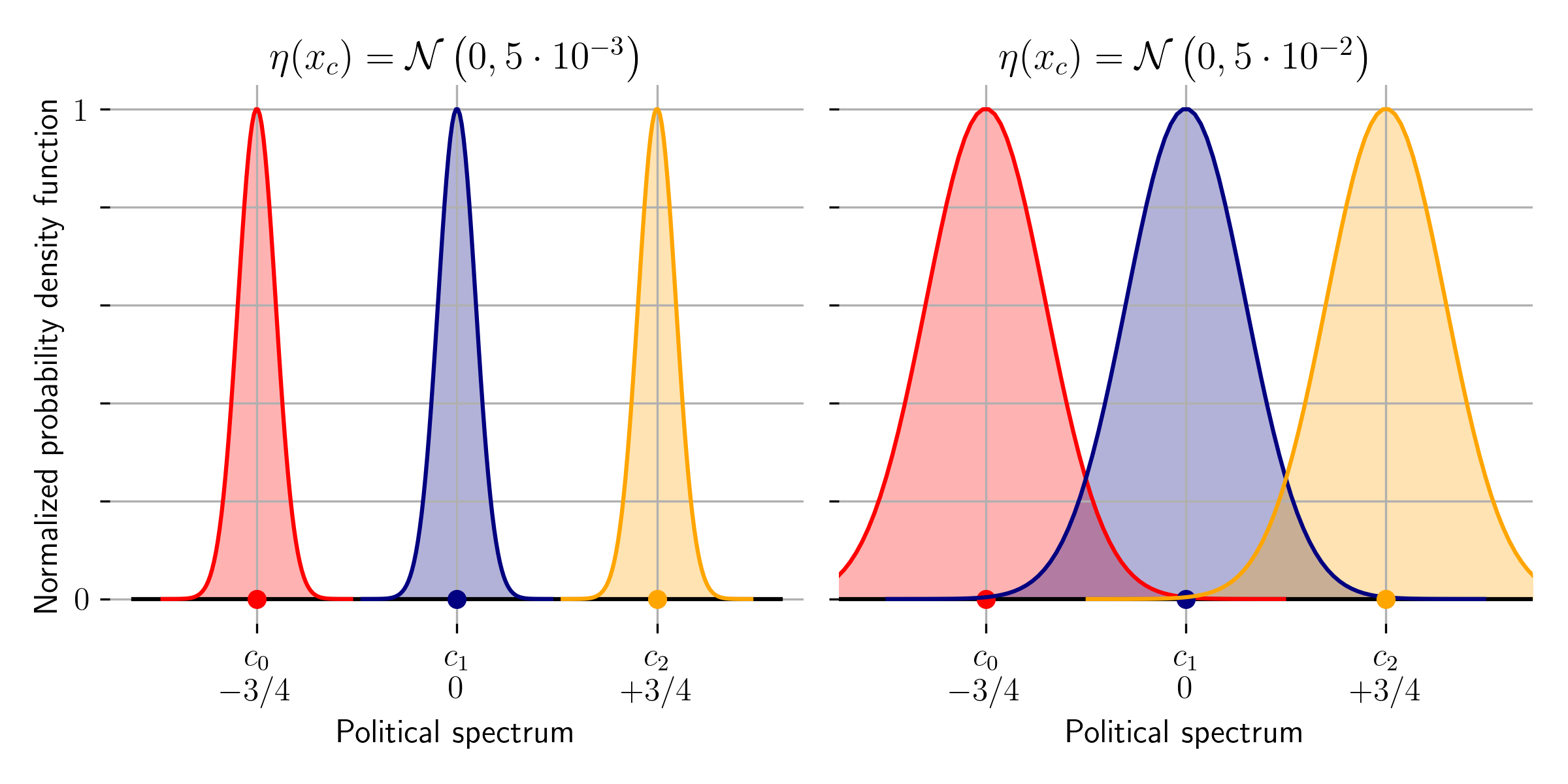
Figure 1: An example of the positions of candidates in nearly-single-peaked electorates. The election involves 3 parties $\{c_{0},c_{1},c_{2}\}$. The left plot shows the distribution of candidates’ positions when noise variance is low. It shows that it is unlikely to swap adjacent candidates in the left-to-right order; hence, preferences are likely to remain single-peaked with respect to the axis $[c_{0},c_{1},c_{2}]$. The right plot shows the effect of noise with high variance: the intersections of the distributions can potentially make candidates swap, creating non-single-peaked preferences. The higher the variance of the noise, the higher the chances of swapping adjacent candidates, and the higher the swap distance of the electorate from being perfectly single-peaked.

A manipulator can spread information supporting $c^{*}$ among voters. Formally, we suppose that voters are arranged on the nodes of a social network $G=(V,E,p)$, where $E$ is the set of edges $(u,v)$ connecting voter $u$ to voter $v$, and $p(u,v)\in[0,1]$ encodes the strength of this relationship, namely how probable is that the information that $u$ sends to $v$ affects the opinion of $v$. The manipulator is then supposed to select a subset $S$ of voters, of size not larger than a given budget $B$, from which the information is sent. As most of the previous literature about election manipulation through social networks [36, 1, 19] we assume that information spreads through the network according to the Independent Cascade Model [29]: it starts with $S_{0}=S$ and, at each time step $t$, if $S_{t-1}$ is not empty, each voter $u$ in $S_{t-1}$ sends the information to each neighbor $v$ that has not been yet affected, and this neighbor $v$ is affected, and hence inserted in $S_{t}$, with probability $p(u,v)$. When a voter $v$ is affected by the news spread by the manipulator (i.e., $v$ belongs to $S_{t}$ for some $t\geq 0$), his belief is updated. Specifically, the voter’s position is moved by a constant amount $\delta$ towards the position (in her view) of the target candidate. If the voter is closer than $\delta$ to the position of $c^{*}$, then she simply moves to $x_{c^{*}}^{v}$. Formally, the voter’s new position $\hat{x}_{v}$ is $\hat{x}_{v}=x_{v}+\min(\delta,|x^{v}_{c^{*}}-x_{v}|)\cdot{\mathop{\mathrm{sign}}}(x^{v}_{c^{*}}-x_{v})$.

As in previous literature [36, 1, 20, 19], we assume that the goal of the manipulator is to choose the set of seed $S$ of size at most $B$ that maximizes the increment in the margin of victory of $c^{*}$. Specifically, the goal of the manipulator is to maximize the expected change of margin of victory $\Delta MoV(S)=|V^{*}_{c^{*}}|-\max_{c\neq c^{*}}|V^{*}_{c}|-\left(|V_{c^{*}}|-\max_{c\neq c^{*}}|V_{c}|\right)$, where, by $|V_{c}|$ and $|V_{c}^{*}|$, we mean, respectively, the number of votes for the candidate $c$ before and after the manipulation. Essentially $\Delta MoV$ is the increase of the advantage of $c^{*}$ over its best opponent before and after the manipulation (that is guaranteed to be always non-negative). Note that the manipulator knows exactly the real position of candidates and of the voters, but she does not know the voters’views.

It is not hard to see that by considering the special case of zero-noise, only two candidates and $\delta$ large enough to guarantee that the least preferred candidate becomes the most preferred candidate for each voter $v$ activated by the spread of information, our model reduces to the one considered in [36]. Hence, the hardness result described there for the election manipulation problem clearly extends to our model. For this reason, in the rest of this work we only look for algorithms able to approximate the optimal choice of the manipulator. Specifically, we say that an algorithm is $\alpha$-approximate, for $\alpha\leq 1$ if it always returns a set of seeds $S$ such that ${\mathop{\mathbb{E}}}[\Delta MoV(S)]\geq\alpha{\mathop{\mathbb{E}}}[\Delta MoV(S^{*})]$, where $S^{*}=\arg\max_{S}{\mathop{\mathbb{E}}}[\Delta MoV(S)]\colon|S|\leq B$ is the optimal seed.

In this work we will also consider an extension of previous models: we allow the manipulator to run a multi-round campaign, by choosing in each round the seeds from which the information spreads, and the electorate evolves accordingly.

We next introduce two tools that will turn out to be particularly useful in the design of our algorithms. The first one consists in an algorithm for finding an approximation to the optimal solution for the Influence Maximization problem: given a budget $B$, a network $G=(V,E)$ and a weight $w(v)$ for each vertex $w$, find the subset $S^{*}\subseteq V$ of size at most $B$ that maximizes the expected total weight of vertices in $A(S^{*})$, that is the vertices affected by the information sent from $S^{*}$ and spread according to the Independent Cascade model, i.e., $S^{*}=\arg\max_{S}{\mathop{\mathbb{E}}}\left[\sum_{v\in A(S)}w(v)\right]$. It is well-known (cf. [29]) that a simple hill-climbing algorithm equipped with Monte Carlo simulations for the estimation of the expectation of random variables is able to return a set of seeds $S$ that provides a $\left(1-\frac{1}{e}-\varepsilon\right)$-approximation of the expected influence of the optimal choice of seeds $S^{*}$.

The second useful tool is given by the PageRank measure [17]. It is a measure of importance of nodes, that evaluates the importance of a node with respect to the importance of its neighbors. Specifically, the page rank $r(v)$ of a node $v$ in a graph $G=(V,E)$ is computed as $\frac{s}{|N_{v}|}\sum_{u\in N_{v}}r(u)+\frac{1-s}{|V|}\sum_{u\in V}r(u)$, where $N_{v}$ is the set of neighbors of $v$ in $G$, and $s$ is a factor in $[0,1]$ weighting these two contributions. It is well-known that by repeatedly applying this update rule we will eventually converge to fixed point values (that is, values that do not change after a further application of the update rule), that we will take as the PageRank measure of these nodes.

3 Approximation Algorithm

We here propose a greedy algorithm, that returns a constant approximation of the optimal solution to the Election Manipulation problem in the setting described above whenever the view of voters corresponds to the real position of candidates. The design of the algorithm directly mimics the ones proposed in [36, 19]. The crux of the algorithm is identifying the voters that, if influenced, will change their minds and vote for the target candidate $c^{*}$. Then, the problem is solved by simply computing the set of seeds that maximizes the weighted influence maximization [29] for which weights 1 are assigned to such voters and 0 to all the other nodes. Indeed, nodes that already supports the target candidate can be useful for spreading information, but reaching them will not modify the margin of victory of the target candidate; similarly, influencing a voter that cannot be convinced to vote for the target candidate apparently cannot improve the margin of victory. Unfortunately, influencing a voter that will never vote for $c^{*}$ after the manipulation is not that pointless: even if the number of votes of the target candidate does not increase, this voter may change her preferred candidate and erode votes for the best opponent of the target candidate, possibly increasing the margin of victory of $c^{*}$. So we need to prove that, even if this strategy is not accounted by our algorithm (i.e., it only focuses on influencing nodes that can be made to support the target candidate but do not actually do), we still achieve a constant approximation whenever the campaign for the target candidate does not advantage other candidates more than the target itself.

Since our approximation algorithm relies on the influence maximization algorithm discussed above, it is easy to see that its computational complexity is $O\left(B\cdot|V|\cdot MI\right)$, where $B$ is the budget, $|V|$ is the number of nodes in the graph, and $MI$ is the cost of estimating the marginal influence of a node via Monte Carlo simulations, that depends on the margin of error that one is willing to accept in the computed estimation. Proposition 1 proves that $MI$ also polynomially depends on the size of the input, allowing us to conclude that our algorithm is polynomial.

Proposition 1

Let $P$ be a weighted influence maximization problem with the following properties:

• $n$ is the number of nodes of the graph;

• for $N\leq n$ nodes $v_{1},...,v_{N}$, the weights are $w(v_{1})=...=w(v_{N})=1$;

• for $n-N$ nodes $v_{N+1},...,v_{n}$ the weights are $w(v_{N+1})=...=w(v_{n})=0$.

That is, $P$ is an influence maximization problem in which nodes $v_{N+1},...,v_{n}$ can be ignored in the final result.

Let $A$ be the set of seed nodes that start the diffusion process. Assume that $A$ contains at least one node $v$ such that $w(v)=1$. Let $\sigma_{w}(A)$ be the expected sum of weights of influenced nodes at the end of the diffusion dynamic (i.e., the expected number of infected nodes ignoring the nodes with weight 0).

If the diffusion process starting from $A$ is simulated independently at least $\frac{N^{2}}{\epsilon^{2}}\cdot ln\left(\frac{1}{\lambda}\right)$ times, then the average number of influenced nodes with weight 1 over these simulations is a $(1\pm\epsilon)$-approximation to $\sigma_{w}(A)$, with probability at least $1-2\lambda^{2}$.

Proof

Assume that the diffusion process is repeated $T\geq\frac{N^{2}}{\epsilon^{2}}\cdot ln\left(\frac{1}{\lambda}\right)$ times.

Let $X_{1},X_{2},...,X_{T}\in[0,1]$ be the fraction of influenced nodes with weight 1 in each of these runs. The estimate of $\sigma_{w}(A)$ is

$$\hat{\sigma}_{w}(A)=\frac{N}{T}\sum_{i=1}^{T}X_{i}$$

Writing $X=\sum_{i=1}^{T}X_{i}$, then $E[X]=\frac{T}{N}\sigma_{w}(A)$. Standard bounds (e.g., Theorem 2.3 from [28]) give that

$$Pr\left(\lvert X-\frac{T}{N}\sigma_{w}(A)\rvert\geq T\gamma\right)\leq 2e^{-2T\gamma^{2}}\forall\gamma\geq 0$$ (1)

Considering $\gamma=\frac{\epsilon}{N}\sigma_{w}(A)$, rearranging the left side of inequality 1 we get

$$Pr\left(\lvert X\cdot\frac{N}{T}-\sigma_{w}(A)\rvert\geq\epsilon\sigma_{w}(A)\right)$$

and rearranging the right side of inequality 1 we get

$$2e^{-2T\gamma^{2}}\leq 2e^{-2ln\left(\frac{1}{\lambda}\right)\sigma^{2}_{w}(A)}\leq 2e^{-2ln\left(\frac{1}{\lambda}\right)}=2\lambda^{2}$$

where the last inequality holds if $\sigma_{w}(A)\geq 1$, which is true since $A$ contains at least one node $v$ such that $w(v)=1$.∎

Moreover, observe that the set of influencers returned by our algorithm has a size that does not exceed the budget, and hence feasible. We next show that it returns a constant approximation of the optimal seed set whenever the view of all voters coincides with candidates’ real positions and the campaign for the target candidate does not advantage more other candidates than the target itself. Specifically, let $X(S)$ be the expected maximum – among all candidates $c\neq c^{*}$ – of the number of voters that do not vote for $c$ and they will do after receiving a message supporting candidate $c^{*}$ starting from nodes in $S$ (where the expectation is taken over the probabilities of receiving this message). Then we have the following theorem.

Theorem 3.1

The set of influencers $\hat{S}\subseteq V$ returned by our algorithm is such that ${\mathop{\mathbb{E}}}[\Delta MoV(\hat{S})]+X(\hat{S})\geq\frac{1}{3}\cdot\left(1-\frac{1}{e}\right)\cdot max_{S}{\mathop{\mathbb{E}}}[\Delta MoV(S)]$ whenever $x_{c}^{v}=x_{c}$ for each $v\in V$ and each $c\in C$. Hence, our algorithm returns a constant approximation whenever $X(\hat{S})=O({\mathop{\mathbb{E}}}[\Delta MoV(\hat{S})])$.

Proof

Given $G=(V,E,p)$, the corresponding live graph is a graph $G^{\prime}$ over $V$ in which each edge $e\in E$ belongs to $G^{\prime}$ with probability $p(e)$. Observe that there are $2^{|E|}$ possible live graphs, and let us denote with $\mathcal{G}$ the set containing all these live graphs. Moreover we can associate a distribution $\mathcal{P}\colon\mathcal{G}\rightarrow[0,1]$ to these live graphs, with $\mathcal{P}(G_{i})=\prod_{e\in G^{\prime}}p(e)\prod_{e\notin G^{\prime}}(1-p(e))$ for each $G_{i}\in\mathcal{G}$. Given a live graph $G_{i}$ and a seed set $S$, we denote with $f(S,i)$ the number of nodes reachable from the seed set $S$ in the live graph $G_{i}$. It is immediate to see that the expected number of influenced nodes in the graph, starting the diffusion from the seed set $S$, is simply $f(S)=\mathop{\mathbb{E}}_{\mathcal{P}}\left[f(S,i)\right]$.

Recall that $M$ is the set of voters that do not vote for $c^{*}$ but will do if influenced. Let $V_{c}$ be the set of voters that vote for candidate $c$ before the manipulation, and $\overline{M}_{c}$ be those voters that do not vote for $c$, but they will vote for $c$ if they receive a message supporting $c^{*}$, i.e., if they move their belief of at most $\delta$ towards $x_{c^{*}}^{v}$. Note that $M_{c}\cap V_{c^{*}}$ must be empty, since it is impossible to make a voter that prefers $c^{*}$ to change her mind through a message supporting $c^{*}$.

Moreover, let $\hat{S}$ be the seed set returned by our algorithm, and $S^{*}$ be an optimal solution maximizing the expected change of margin of victory.

After the manipulation due to the influencers $\hat{S}$, the increment in the margin of victory between $c^{*}$ and any other candidate $c_{i}\neq c^{*}$ can be expressed (considering the diffusion over the graph $G_{y}$) as $g_{c^{*}}(\hat{S},y,c_{i})$ and observe that

$$\sum_{v\in M-V_{c_{i}}}\chi(v,\hat{S},y)+2\sum_{v\in M\cap V_{c_{i}}}\chi(v,\hat{S},y)\geq$$

$$g_{c^{*}}(\hat{S},y,c_{i})\geq\sum_{v\in M-V_{c_{i}}}\chi(v,\hat{S},y)+2\sum_{v\in M\cap V_{c_{i}}}\chi(v,\hat{S},y)$$

$$\qquad-\sum_{v\in\overline{M}_{c_{i}}}\chi(v,\hat{S},y)$$

$$\geq\sum_{v\in M-V_{c_{i}}}\chi(v,\hat{S},y)+2\sum_{v\in M\cap V_{c_{i}}}\chi(v,\hat{S},y)-\max_{c\neq c^{*}}\sum_{v\in\overline{M}_{c}}\chi(v,\hat{S},y),$$

where $\chi(v,\hat{S},y)$ is 1 if node $v$ is reachable from nodes in $\hat{S}$ in the live graph $G_{y}$, else 0. The change of margin of victory in the live graph $G_{y}$ is then

$$\Delta MoV(\hat{S},y)=\min_{c_{j}\neq c^{*}}\left\{g_{c^{*}}(\hat{S},y,c_{j})-|V_{c_{j}}|+\max_{c_{i}\neq c^{*}}|V_{c_{i}}||\right\}$$

and the expected change of margin of victory is $\mathop{\mathbb{E}}_{y}\left[\Delta MoV(\hat{S},y)\right]$. Note that

$$\sum_{v\in M-V_{c_{i}}}\chi(v,\hat{S},y)+2\sum_{v\in M\cap V_{c_{i}}}\chi(v,\hat{S},y)=f(\hat{S},y,M)+f(\hat{S},y,M\cap V_{c_{i}}),$$

where $f(S,y,A)$ is the number of nodes in $A$ reachable from $S$ in the live graph $G_{y}$. Then we have that

$$f(\hat{S},y,M)+\min_{c_{j}\neq c^{*}}\left[f(\hat{S},y,M\cap V_{c_{j}})-|V_{c_{j}}|+\max_{c_{i}\neq c^{*}}|V_{c_{i}}|\right]\geq$$ (2)

$$\Delta MoV(\hat{S},y)\geq f(\hat{S},y,M)$$

$$+\min_{c_{j}\neq c^{*}}\left[f(\hat{S},y,M\cap V_{c_{j}})-|V_{c_{j}}|+\max_{c_{i}\neq c^{*}}|V_{c_{i}}|\right]-\max_{c\neq c^{*}}\sum_{v\in\overline{M}_{c}}\chi(v,\hat{S},y).$$

By definition, our algorithm greedily maximizes the submodular function $\mathop{\mathbb{E}}_{y}\left[f(\cdot,y,M)\right]$. In fact, it maximizes the expected sum of the weights of the influenced nodes in the derived influence maximization problem; but weights are defined such that the expected sum of influenced nodes is exactly the expected number of influenced nodes in $M$, that is $\mathop{\mathbb{E}}_{y}\left[f(\cdot,y,M)\right]$. Hence, if $S^{\prime}=\arg\max_{A}\mathop{\mathbb{E}}_{y}\left[f(A,y,M)\right]$, then

$$\mathop{\mathbb{E}}_{y}\left[f(\hat{S},y,M)\right] \geq\left(1-\frac{1}{e}\right)\cdot\mathop{\mathbb{E}}_{y}\left[f(S^{\prime},y,M)\right]$$ (3)

$$\geq\left(1-\frac{1}{e}\right)\cdot\mathop{\mathbb{E}}_{y}\left[f(S^{*},y,M)\right]$$

where the first inequality holds because of the guarantees of the algorithm solving weighted influence maximization, whereas the second inequality holds because $S^{\prime}$ maximizes $\mathop{\mathbb{E}}_{y}\left[f(\cdot,y,M)\right]$ by definition.

Let $c(\hat{S},y)=\arg\min_{c_{i}}f(\hat{S},y,M\cap V_{c_{i}})-|V_{c_{i}}|$ be the candidate achieving the minimum in the definition of $\Delta MoV(\hat{S},y)$ in (2). Note that for any candidate $c_{i}$, $f(\hat{S},y,M)\geq f(S,y,M\cap V_{c_{i}})$, simply because $M\cap V_{c_{i}}\subseteq M$. Hence, for $S\in\{S^{*},\hat{S}\}$

$$\mathop{\mathbb{E}}_{y}\left[f(S^{*},y,M)\right]\geq\mathop{\mathbb{E}}_{y}\left[f(S^{*},y,M\cap V_{c(S,y)})\right]$$ (4)

By (4) we get

$$\mathop{\mathbb{E}}_{y}\left[f(S^{*},y,M)\right] \geq\frac{1}{3}\left(\mathop{\mathbb{E}}_{y}\left[f(S^{*},y,M)\right]\right.$$ (5)

$$+\mathop{\mathbb{E}}_{y}\left[f(S^{*},y,M\cap V_{c(S^{*},y)})\right]$$

$$+\left.\mathop{\mathbb{E}}_{y}\left[f(S^{*},y,M\cap V_{c(S,y)})\right]\right)$$

Moreover,

$$\mathop{\mathbb{E}}_{y}\left[f(\hat{S},y,M)+f(\hat{S},y,M\cap V_{c(\hat{S},y)})\right]\geq\mathop{\mathbb{E}}_{y}\left[f(\hat{S},y,M)\right]$$ (6)

$$\geq\frac{1}{3}\left(1-\frac{1}{e}\right)\cdot\left(\mathop{\mathbb{E}}_{y}\left[f(S^{*},y,M)\right]+\mathop{\mathbb{E}}_{y}\left[f(S^{*},y,M\cap V_{c(S^{*},y)})\right]\right.$$

$$\qquad\left.+\mathop{\mathbb{E}}_{y}\left[f(S^{*},y,M\cap V_{c(S,y)})\right]\right)$$

where the first inequality holds because the left hand side includes an extra non-negative term, and the second inequality derives from inequalities 5 and 3. Also note that $\mathop{\mathbb{E}}_{y}\left[\max_{c\neq c^{*}}\sum_{v\in\overline{M}_{c}}\chi(v,\hat{S},y)\right]=X(\hat{S})$. We can bound the margin of victory of $\hat{S}$ as follows (for simplicity, we will write “$\min_{c_{j}}$” for “$\min_{c_{j}\neq c^{*}}$”, and the same for “$\max_{c_{j}}$”):

$$\mathop{\mathbb{E}}_{y}\left[\Delta MoV(\hat{S},y)\right]+X(\hat{S})$$

$$\geq\mathop{\mathbb{E}}_{y}\left[f(\hat{S},y,M)+\min_{c_{j}}\left(f(\hat{S},y,M\cap V_{c_{j}})-|V_{c_{j}}|\right)+\max_{c_{i}}|V_{c_{i}}|\right]$$ (by (2))

$$=\mathop{\mathbb{E}}_{y}\left[f(\hat{S},y,M)+f(\hat{S},y,M\cap V_{c(\hat{S},y)})\right]+\mathop{\mathbb{E}}_{y}\left[\max_{c_{i}}|V_{c_{i}}|-|V_{c(\hat{S},y)}|\right] c(\hat{S},y)$$ (by definition of )

$$\geq\frac{1}{3}\left(1-\frac{1}{e}\right)\cdot\mathop{\mathbb{E}}_{y}\biggl{[}f(S^{*},y,M)+f(S^{*},y,M\cap V_{c(S^{*},y)})$$

$$\qquad+f(S^{*},y,M\cap V_{c(\hat{S},y)})\biggr{]}+\mathop{\mathbb{E}}_{y}\left[\max_{c_{i}}|V_{c_{i}}|-|V_{c(\hat{S},y)}|\right]$$ (by (6))

$$\geq\frac{1}{3}\left(1-\frac{1}{e}\right)\cdot\mathop{\mathbb{E}}_{y}\biggl{[}f(S^{*},y,M)+f(S^{*},y,M\cap V_{c(S^{*},y)})$$

$$\qquad+f(S^{*},y,M\cap V_{c(\hat{S},y)})+\max_{c_{i}}|V_{c_{i}}|-|V_{c(\hat{S},y)}|\biggr{]}$$ (1/3(1-1/e) multiplies every term)

$$=\frac{1}{3}\left(1-\frac{1}{e}\right)\cdot\mathop{\mathbb{E}}_{y}\biggl{[}f(S^{*},y,M)+f(S^{*},y,M\cap V_{c(S^{*},y)})$$

$$\qquad+f(S^{*},y,M\cap V_{c(\hat{S},y)})+\max_{c_{i}}|V_{c_{i}}|-|V_{c(\hat{S},y)}|+|V_{c(S^{*},y)}|-|V_{c(S^{*},y)}|\biggr{]}$$ (add and subtract the same quantity)

$$=\frac{1}{3}\left(1-\frac{1}{e}\right)\cdot\mathop{\mathbb{E}}_{y}\biggl{[}f(S^{*},y,M)+\min_{c_{j}}\left(f(S^{*},y,M\cap V_{c_{j}})-|V_{c_{j}}|\right)$$

$$\qquad+f(S^{*},y,M\cap V_{c(\hat{S},y)})+\max_{c_{i}}|V_{c_{i}}|-|V_{c(\hat{S},y)}|+|V_{c(S^{*},y)}|\biggr{]} c(S^{*},y)$$ (by definition of )

$$\geq\frac{1}{3}\left(1-\frac{1}{e}\right)\cdot\biggl{(}\mathop{\mathbb{E}}_{y}[\Delta MoV(S^{*},y)]+\mathop{\mathbb{E}}_{y}\biggl{[}f(S^{*},y,M\cap V_{c(\hat{S},y)})$$

$$\qquad+|V_{c(S^{*},y)}|-|V_{c(\hat{S},y)}|\biggr{]}\biggr{)}$$ (by (2))

By definition of $c(S^{*},y)$, $f(S^{*},y,M\cap V_{c(S^{*},y)})-|V_{c(S^{*},y)}|\leq f(S^{*},y,M\cap V_{c(\hat{S},y)})-|V_{c(\hat{S},y)}|$, and hence

$$|V_{c(S^{*},y)}|-|V_{c(\hat{S},y)}|\geq f(S^{*},y,M\cap V_{c(S^{*},y)})-f(S^{*},y,M\cap V_{c(\hat{S},y)})$$ (7)

We can conclude that

$$\mathop{\mathbb{E}}_{y}[\Delta MoV(\hat{S},y)]+X(\hat{S})$$

$$\geq\frac{1}{3}\left(1-\frac{1}{e}\right)\cdot\biggl{(}\mathop{\mathbb{E}}_{y}[\Delta MoV(S^{*},y)]+\mathop{\mathbb{E}}_{y}\biggl{[}f(S^{*},y,M\cap V_{c(\hat{S},y)})$$

$$\quad+f(S^{*},y,M\cap V_{c(S^{*},y)})-f(S^{*},y,M\cap V_{c(\hat{S},y)})\biggr{]}\biggr{)}$$ (by (7))

$$=\frac{1}{3}\left(1-\frac{1}{e}\right)\cdot\biggl{(}\mathop{\mathbb{E}}_{y}[\Delta MoV(S^{*},y)]+\mathop{\mathbb{E}}_{y}\biggl{[}f(S^{*},y,M\cap V_{c(S^{*},y)})\biggr{]}\biggr{)}$$

$$\geq\frac{1}{3}\left(1-\frac{1}{e}\right)\cdot\mathop{\mathbb{E}}_{y}[\Delta MoV(S^{*},y)]$$ (since f is non-negative)

Thus if $X(\hat{S})=O(\mathop{\mathbb{E}}_{y}[\Delta MoV(\hat{S},y)])$, then there is a constant $c$ such that $X(\hat{S})\leq c\cdot\mathop{\mathbb{E}}_{y}[\Delta MoV(\hat{S},y)]$, and thus

$$\mathop{\mathbb{E}}_{y}[\Delta MoV(\hat{S},y)]\geq\frac{1}{3(c+1)}\left(1-\frac{1}{e}\right)\cdot\mathop{\mathbb{E}}_{y}[\Delta MoV(S^{*},y)],$$

and thus a constant approximation. ∎

Note that in case of nearly-single-peaked electorates the algorithm still works, but its performances in terms of $\Delta MoV(\cdot)$ depend on the amount of noise: the higher the noise, the more the inconsistency between reality and blurred views of the voters, the lower the effectiveness of the manipulation since the manipulator estimates wrong weights $w(v)$ for each voter $v\in V$.

4 The Heuristics

The approximation algorithm presented in the previous section provides a formal guarantee of the quality of the solution. However, it inherits from the weighted influence maximization algorithm used as black box the computational drawbacks of being computationally expensive, even if it is polynomial in the size of the input. Specifically, the proposed algorithm requires a large number of simulations in order to estimate the marginal influence of each node (see Proposition 1). Even if faster algorithms have been proposed for the influence maximization algorithm (see, e.g., [14]), the influence maximization algorithm is often solved in practice through fast heuristics based only on the structure of the network: they, indeed, assign scores to the nodes in the graph defining their “importance”, and then they simply return the nodes with the highest scores.

In this work, we propose to extend this approach in order to encompass the problem of election manipulation. Specifically, this work introduces several heuristics in that sense: they are based on both the structure of the networks and centrality metrics adapted to the election context. We next present in details these heuristics.

The core idea involves computing the distance on the political spectrum of a voter from the target candidate. Among the supporters of candidates other than the target $c^{*}$, the closer is this voter to $c^{*}$, the higher is the importance of this voter for manipulation purposes. However, the score must also take into account social influence and the ability of a (possibly useless for manipulation purposes) voter to influence other (useful for manipulation purposes) voters. These ideas lead to two different classes of heuristics that we will describe below, and whose performances are described in the next section.

Scoring-based Heuristics.

The first proposed class of heuristics considers the nodes in the neighbourhood $N(v)$ of each voter $v$ and their inclination to support the target candidate. Different heuristics in this class can be distinguished by how the neighborhood $N(v)$ is defined. For example,

• we can consider in $N(v)$ only neighbours up to a given distance. For instance, setting this limit to 1, we consider only $v$’s friends; setting it to 2, we consider $v$’s friends and, in turn, their friends, too.

• $N(v)$ can be limited by a maximum number of nodes to consider, regardless of the distance. One can consider the neighbours at increasing distances from $v$, as long as the number of neighbours does not exceed a given threshold.

• we can limit $N(v)$ by both the constraints above.

Given $N(v)$, the higher the number of friends of $v$, the higher is the probability of exerting social influence. Clearly, this probability also depends on the distance from $v$, since neighbors of $v$ only require that influence from $v$ is successful, while for a friend of a friend $u$ of $v$ we require that not only the influence of $v$ but also the influence of $u$ is successful. These considerations justify the definition of a first score $s_{G}(v)=\sum_{u\in N(v)}1/d(v,u)$ for the node $v$ purely based on the structure of the network $G$, where $d(v,u)$ is the length of the shortest path linking $v$ to $u$.

We also consider political information about voters in the neighbourhood of $v$: indeed, we define $s_{P}(v)=\sum_{u\in N(v)\cup\{v\}:F[d_{P}(u,c^{*})]=1}w(v,u)\cdot 1/d_{P}(u,c^{*})$ for the node $v$, where $d_{P}(u,c^{*})$ is a political distance function, that measures the distance on the political spectrum between $c^{*}$ and voter $u$; $F[\cdot]$ is a custom filter function, allowing to discard nodes depending on the distance $d_{P}$ (e.g., we may discard nodes $u$ such that $d_{P}(u,c^{*})=0$, which means that they already vote for $c^{*}$); $w(v,u)$ is the product of the probabilities of the edges along the shortest path from $v$ to $u$. In this way, nodes that are more likely to be influenced by $v$ are assigned a high weight. We assume that $w(v,v)=1$. Hence, $s_{P}(v)$ is high when the neighbourhood of $v$ is large, neighbours’ political positions are not too far from $c^{*}$’s, and $v$ is likely to influence his neighbourhood, as desired.

We can then achieve different heuristics by combining these two scores in different ways. The following are possible combinations:

• $s_{1}(v)=(s_{G}(v),s_{P}(v))$

• $s_{2}(v)=(s_{P}(v),s_{G}(v))$

• $s_{3}(v)=\alpha\hat{s}_{P}(v)+(1-\alpha)\hat{s}_{G}(v)$

where $\hat{s}_{G}(v)$ is $s_{G}(v)$ divided by the standard deviation of $s_{G}(u)$ over all the nodes $u\in V$; similarly for $\hat{s}_{P}(v)$. By using $s(v)=(X,Y)$, we mean that when comparing the scores of two nodes $u$ and $v$, the comparison is performed on the value of $X$, whereas $Y$ breaks ties. Having defined the score of the nodes, the algorithm greedily chooses the $B$ nodes $v$ with the highest score $s(v)$.

PageRank-based Heuristics.

Motivated by the fact that PageRank is a fast heuristic that embodies the structure of the whole network, this work also suggests a second fast heuristic based on a special version of PageRank specifically thought for the problem of election manipulation. In particular, we observe that while the original PageRank shares the importance of a node among all its neighbors with probability $1-s$, and among all nodes with probability $s$, this does not makes really sense in our setting, since we already known that there are nodes that are more useful to the goal (i.e., the ones that may be lead to vote for $c^{*}$), and others that are less useful to this purpose (i.e., the ones that already vote for the desired candidate or the ones that cannot be made to vote for $c^{*}$).

Our idea is to share the rank of node $u$, by first assigning to each neighbor $v$ a weight $z_{u}(v)\geq 0$, quantifying how strongly $v$ positively influences other nodes to switch to $c^{*}$, and to share the PageRank of $u$ among its neighbors proportionally to their weight. It is not hard to check that this modification does not affect the Markovian nature of PageRank computation, and hence the fact that it eventually converges to a stable set of values.

How should the weights be selected? Scores defined above already provide a measure of how much the social influence of the node serves to the purpose of the manipulator. Hence, we can for example set $z_{u}(v)=s_{3}(v)$ for a specific value of $\alpha$. Another variant of this heuristics, can be achieved by including in the weight $z_{u}(v)$ also information related to the diffusion probabilities, i.e., $z_{u}(v)=s_{3}(v)\cdot p(u,v)$.

In this way, this heuristics tends to assign a high score to nodes:

• generally important for the diffusion in the network (inheriting PageRank properties about influence maximization), and

• with a high probability of influencing their neighbourhood, and

• whose neighbourhood does not already support $c^{*}$ (need to choose an appropriate filter function $F[\cdot]$), and

• whose neighbourhood contains nodes that are not too far from the target candidate on the political spectrum (thus, they are willing to change their mind in favour of $c^{*}$).

The Full List of Heuristics.

Based on the above ideas, we next describe the heuristics that we considered in this work.

All heuristics adopting the neighbourhood score use the following distance function:

$$d_{P}(u,c^{*})=\begin{cases}0&\text{if }u\text{ votes for $c^{*}$ before the manipulation}\\ |x_{u}-x_{c^{*}}|&\text{otherwise}\end{cases}$$

This highlights the reasons for which this heuristics should perform worse in nearly-single-peaked scenarios: when ${\eta}\neq 0$, $x_{c^{*}}\neq x^{v}_{c^{*}}$ and the value of $d_{P}(u,c^{*})$ does not reflect the distance from $c^{*}$ perceived by the voter $u$ (and the manipulator could also guess that a voter votes for $c^{*}$ when he does not actually do).

In addition, all the versions of the algorithms adopting the neighbourhood score use the following filter function:

$$F[a]=\begin{cases}1&\text{if }a>0\\ 0&\text{otherwise}\end{cases}$$

This means that when computing the political scores $s_{P}(v)$, the algorithms discard all the voters that already vote for $c^{*}$ in the neighbourhood $N(v)$.

The neighbourhood $N(u)$ was limited to consider (1) friends of node $u$ or (2) friends of $u$ and friends of $u$’s friends. No limit was applied to the size of the neighbourhood. Moreover, the variants of the algorithms consider three ways of combining scores $s_{P}$ and $s_{G}$ to obtain the score $s$, namely $s=(s_{G},s_{P})$, $s=(s_{P},s_{G})$, $s=\alpha\hat{s}_{P}+(1-\alpha)\hat{s}_{G}$.

In conclusion, the algorithms based on the neighbourhood heuristic are:

• SPoutdeg. The neighbourhood of a node only considers its friends; the combined score is $s=(s_{G},s_{P})$.

• SPoutdeg_rev. The neighbourhood of a node only considers its friends; the combined score is $s=(s_{P},s_{G})$.

• SPoutdeg_merge0.5. The neighbourhood of a node only considers its friends; the combined score is $s=0.5\cdot\hat{s}_{P}+0.5\cdot\hat{s}_{G}$.

• SPneig2. The neighbourhood of a node considers its friends and friends of friends (2 is the maximum number of hops to reach the nodes in the neighbourhood); the combined score is $s=(s_{G},s_{P})$.

• SPneig2_rev. The neighbourhood of a node considers its friends and friends of friends; the combined score is $s=(s_{P},s_{G})$.

• SPneig2_merge0.5. The neighbourhood of a node considers its friends and friends of friends; the combined score is $s=0.5\cdot\hat{s}_{P}+0.5\cdot\hat{s}_{G}$.

We can now present the variants of the weighted PageRank algorithm that use the neighbourhood score when sharing PageRank among nodes. These are the PageRank heuristics that use the previously defined distance function $d_{P}$ and the previously defined filter function $F$:

• SPpagerank1.0_pos. The scores $s$ use the neighbourhoods considering only the friends of the nodes. In particular, $s=0\cdot\hat{s}_{G}+1\cdot\hat{s}_{P}=\hat{s}_{P}$. pos stands for positive filter $F$.

• SPpagerank0.5_pos. The scores $s$ use the neighbourhoods considering only the friends of the nodes. In particular, $s=0.5\cdot\hat{s}_{G}+0.5\cdot\hat{s}_{P}$. pos stands for positive filter $F$.

• SPpagerank1.0_hop2_pos. The scores $s$ use the neighbourhoods considering the friends of the nodes and the friends of friends. In particular, $s=0\cdot\hat{s}_{G}+1\cdot\hat{s}_{P}$. pos stands for positive filter $F$. hop2 stands for the maximum number of hops to build the neighbourhood.

In addition, there are other two algorithms based on PageRank. Recall that $M$ has been defined as the set of voters that, if influenced, will vote for $c^{*}$. Then we have the following algorithms:

• SPpagerank1.0_manip_eq1. The scores $s$ use the neighbourhoods considering only the friends of the nodes. In particular, $s=\hat{s}_{P}$. The distance function assigns $1$ to manipulable nodes (namely the ones in $M$), $0$ to voters that already vote for $c^{*}$, and $\infty$ to the rest of the voters (this represents the fact that nodes are not manipulable in favour of $c^{*}$). The filter function is

  $$F[a]=\begin{cases}1&\text{if }a=1\\ 0&\text{otherwise}\end{cases}$$

  In the friendly name, manip stands for manipulable and eq1 is a short name for the filter function.

• SPpagerank1.0_manip*_pos. The scores $s$ use the neighbourhoods considering only the friends of the nodes. In particular, $s=\hat{s}_{P}$. The distance function assigns $1$ to manipulable nodes (namely the ones in $M$), $0$ to voters that already vote for $c^{*}$, and

  $$\frac{|x_{v}-x_{c^{*}}|}{|x_{v}-x_{c^{*}}|-|\hat{x}_{v}-x_{c^{*}}|}$$

  to the rest of the voters $v$, where $\hat{x}_{v}$ is the position of voter $v$ if he was influenced. manip* stands for the fact that the algorithm works as SPpagerank1.0_manip_eq1 does but considers the gain (in getting closer to $x_{c^{*}}$) of non-manipulable voters.

Complexity of Heuristics.

To analyze the complexity of the neighbourhood heuristics, Algorithm 1 sketches the main required steps.

Algorithm 1 Neighbourhood heuristic

the graph of voters $G=(V,E)$, the target candidate $c^{*}$

for $v$ in $V$ do

     // Perform a BFS traversal not violating the constraints on the limit of the neighbourhood

     $N(v)=BFS(v)$

     $s_{G}(v)=\sum_{u\in N(v)}1/d(v,u)$

     // $\beta$ is the weight function combining $F$ and $w$

     $s_{P}(v)=\sum_{u\in N(v)}\beta(u,v)/d_{P}(u,c^{*})$

end for

// Standardize the scores for each $v\in V$

$\hat{s}_{G}(v)=s_{G}(v)/STD(s_{G}(\cdot))$

$\hat{s}_{P}(v)=s_{P}(v)/STD(s_{P}(\cdot))$

// Combine $\hat{s}_{G}(v)$ and $\hat{s}_{P}(v)$ for each $v\in V$

$s(v)=...$ $\triangleright$ Depends on the specific score

return $s$

We assume that the function $d_{P}(u,c^{*})$ finds the most preferred candidate of voter $u$. In this way, $d_{P}(u,c^{*})$ can be $0$ if $u$ votes for $c^{*}$, even if the distance between $u$ and $c^{*}$ is not $0$. Hence the complexity of $d_{P}(u,c^{*})$ is $O(m)$, where $m$ is the number of candidates. As explained above, most of the experiments are performed considering that $N(v)$ contains only the friends of $v$; hence $s_{G}(v)=outdeg(v)$ and can be computed in $O(1)$ time with an appropriate representation of the graph. Similarly, $s_{P}(v)$ can be computed in $O(outdeg(v)\cdot m)$. The total cost to compute $s_{G}$ and $s_{P}$ is

$$\sum_{v\in V}O(outdeg(v)\cdot m)=O(|E|\cdot m)$$

The standardization costs $O(|V|)$; hence, the total cost to compute the neighbourhood heuristic is $O(|V|+m\cdot|E|)$.

Compared to the standard algorithm, the weighted version of the PageRank algorithm does not require any substantial extra cost. Thus, for simplicity, the calculations of the computational complexity to compute the PageRank heuristic are based on the original PageRank algorithm. Algorithm 2 sketches the main steps required to calculate PageRank values of the nodes of a given graph.

Algorithm 2 PageRank - computational complexity: $O(k\cdot(|E|+|V|))$

the graph of nodes $G=(V,E)$, the number of iterations $k$, the scaling factor $s$

$r(v)=1/|V|,\forall v\in V$

for $i=1,...,k$ do

     $r^{*}(v)=0,\forall v\in V$

     for $v$ in $V$ do

         // Apply the update rule

         for $u$ in out-neighbours of $v$ do

              $r^{*}(u)\mathrel{+}=r(v)/outdeg(v)\cdot s$

         end for

         $r^{*}(v)\mathrel{+}=(1-s)/|V|$

     end for

     $r(v)=r^{*}(v),\forall v\in V$

end for

return $r$

The update rule for all the nodes requires

$$\sum_{v\in V}\sum_{u\in N^{+}_{v}}O(1)=\sum_{v\in V}O(outdeg(v))=O(|E|)$$

where $N^{+}_{v}$ is the set of out-neighbours of node $v$. At each iteration, an additional cost $O(|V|)$ is required to manage $r$ and $r^{*}$. Since the update rule is applied $k$ times to converge to stable values, the total computational complexity is $O(k\cdot(|E|+|V|))$. Note that this is a naive implementation of the PageRank algorithm. It is presented here only to pose an upper bound to the computational complexity of the PageRank heuristics. In fact, solving the problem by finding a particular eigenvector of a matrix related to the graph can speed up the computations. In fact, the implementation used for the experimental phase relies on scipy’s methods to compute eigenvectors, which are based on ARPACK, a library specifically designed for solving large scale eigenvalue problems. Hence, the actual performances of the algorithm can be much better than implementing Algorithm 2. Moreover, optimized implementations of PageRank can surely scale up to large graphs.

5 Experimental Results

Experimental Setting.

We run extensive experiments to evaluate the algorithms described above both in terms of the effectiveness of the manipulation, as measured by the margin of victory $MoV$ and the change of margin of victory $\Delta MoV$ resulting from the simulated manipulations, and the execution time of the algorithms. As for the valuation of the running time, we used the following software and hardware equipment:

• Windows 10 (listed here for reproducibility of the execution times);

• Python 3.8.10;

• scipy, version 1.8.1 (listed here for reproducibility of the PageRank algorithm).

The details of the hardware environment are:

• RAM: 8 GB;

• CPU: i5-6400, 2.70 GHz.

We stress that we compare Python implementations run on a single core, without any code optimization.

In general we compared different algorithms in election scenarios with a set of voters of sizes 20, 50, and 100. All experiments involved five candidates. Both voters and candidates were assigned positions in the range $[-1,+1]$ chosen uniformly at random. This should create scenarios in which all the parties are almost equally supported by the voters. When dealing with nearly-single-peaked electorates, the noise was chosen to be independent of the positions of the candidates, namely ${\eta}(x_{c})={\eta}$. Specifically, we considered uniform noise ${\eta}=U(-0.2;0.2)$; Gaussian noise with low variance ${\eta}=\mathcal{N}(0;0.08)$; and Gaussian noise with high variance ${\eta}=\mathcal{N}(0;1)$. These values were chosen to test different levels of nearly single-peaked average swap distances. In fact, when normalized with respect to the number of voters, for an election with 20 voters and 5 candidates randomly placed on the political spectrum, the average distances from single-peaked scenarios are $\sim 0.5$, $\sim 1$, and $\sim 2$ swaps (see also Figure 2).

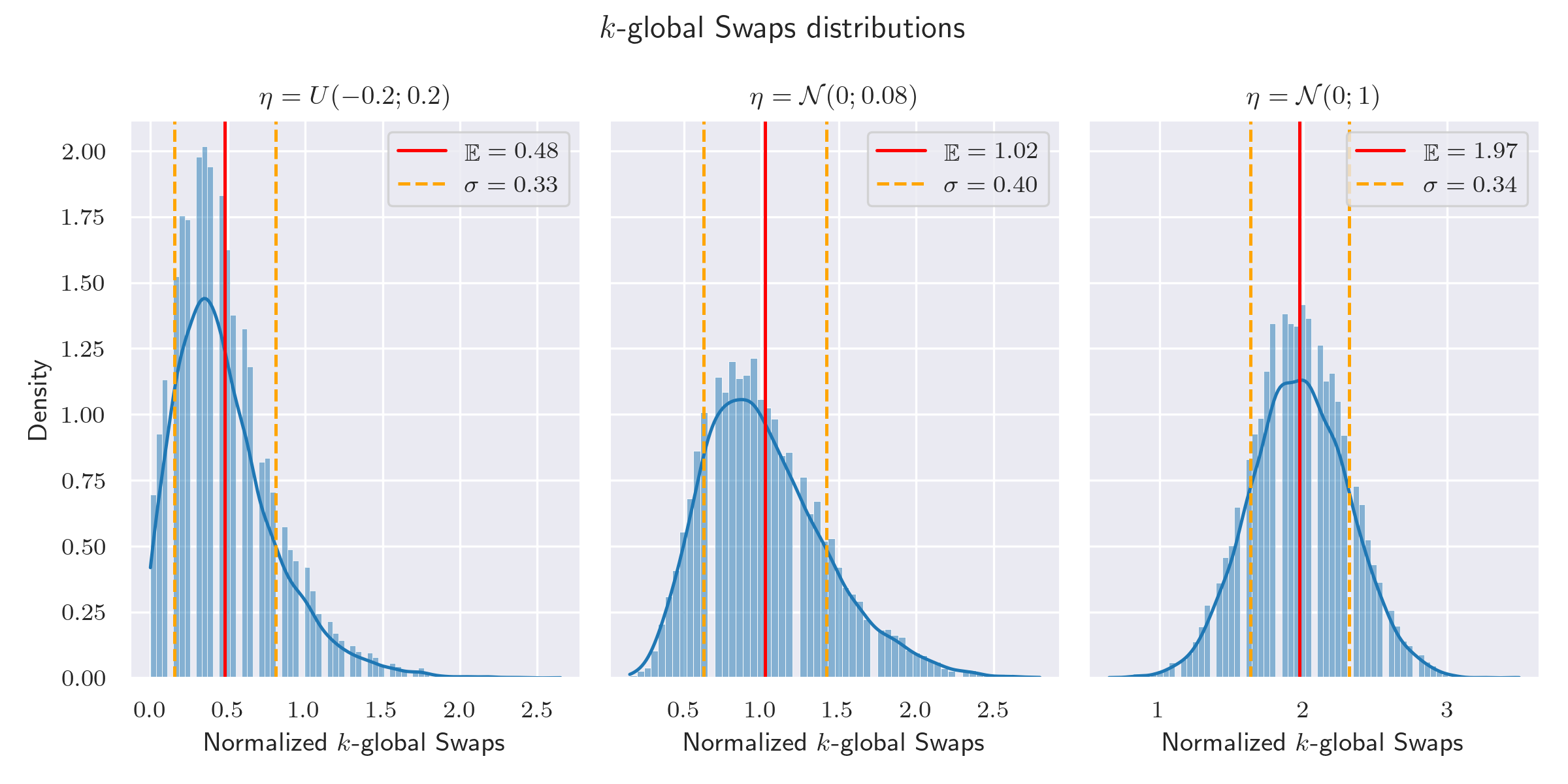
Figure 2: Distributions of $k$-global swaps distances (normalized with respect to 20 voters) for three different noises. Data of the distributions derive from 10000 elections involving 20 voters and 5 candidates placed on the political spectrum uniformly at random. The plots show the average $k$-swap distance (red) and the deviation from the mean (orange).

As for the parameters describing the power of the manipulator, we consider budget $B$ such that $\frac{B}{|V|}\in\{5\%,10\%,15\%\}$; the maximum number of manipulation campaigns was set to 10; the parameter $\delta$ that represents the influenceability of the electorate has been chosen in $\{0.1,0.2,0.3,0.4\}$; the target candidate of the manipulation process was chosen randomly among all the candidates $\{c_{0},c_{1},c_{2},c_{3},c_{4}\}$ unless stated differently.

Monte-Carlo simulations necessary for the approximation algorithm have been repeated 300 times (corresponding to $\lambda=\sqrt{\frac{0.1}{2}}$ and $\epsilon=0.05\cdot\sqrt{2}$ in Proposition 1). Moreover, estimates of $\Delta MoV$ have been evaluated over a number of simulation sufficient to achieve statistical guarantee. Specifically, the number of simulation have been selected according to the following results.

Proposition 2

Let $X_{1},\ldots,X_{T}$ be i.i.d random variables such that $a\leq X_{i}\leq b$ with probability 1, $\forall i\in\{1,...,T\}$. Let $\mu=E[X_{1}]=...=E[X_{T}]$.

The average $\hat{\mu}=1/T\cdot\sum_{i=1}^{T}X_{i}$ is an approximation to $\mu$ with an error smaller than $\epsilon$, with probability at least $1-2\lambda^{2}$, if

$$T\geq\left(\frac{b-a}{\epsilon}\right)^{2}ln\left(\frac{1}{\lambda}\right)$$

Proof

Let $X=\sum_{i=1}^{T}X_{i}$. Applying Hoeffding’s inequality we get:

$$Pr\left(\lvert X-E[X]\rvert\geq\gamma\right)\leq 2\exp\left(-\frac{2\gamma^{2}}{\sum_{i=1}^{T}{(b-a)^{2}}}\right)\forall\gamma>0$$ (8)

Rearranging the left side of (8) we get

$$Pr\left(\lvert\frac{X}{T}-\mu\rvert\geq\frac{\gamma}{T}\right)=Pr\left(\lvert\hat{\mu}-\mu\rvert\geq\frac{\gamma}{T}\right)$$

Choosing $\gamma=T\epsilon$ and rearranging the right side of (8) we get

$$Pr\left(\lvert\hat{\mu}-\mu\rvert\geq\epsilon\right)\leq 2exp\left(-\frac{2\gamma^{2}}{\sum_{i=1}^{T}{(b-a)^{2}}}\right) =2exp\left(-\frac{2}{T(b-a)^{2}}T^{2}\epsilon^{2}\right) \gamma$$ by substituting

$$=2exp\left(-\frac{2}{(b-a)^{2}}T\epsilon^{2}\right)$$

$$\leq 2exp\left(-2ln\left(\frac{1}{\lambda}\right)\right) T$$ by substituting

$$=2\lambda^{2}$$ ∎

Corollary 1

With $\left(\frac{|V|-|V_{c^{*}}|+|V_{\bar{c}}|}{\epsilon}\right)^{2}ln\left(\frac{1}{\lambda}\right)$ simulations, where $|V_{c^{*}}|$ is the number of votes for $c^{*}$ before the manipulation and $|V_{\bar{c}}|$ is the number of votes for the best opponent of $c^{*}$ before the manipulation, we can evaluate the expected $\Delta MoV$ with an error smaller than $\epsilon$, with probability at least $1-2\lambda^{2}$

Proof

Proposition 2 can be used to compute the number of simulations needed to approximate the statistical mean of $\Delta MoV$. The definition of the increment of the margin of victory of the target candidate $c^{*}$ is reported here for convenience:

$$\Delta MoV=|V_{c^{*}}^{*}|-|V_{\hat{c}}^{*}|-\left(|V_{c^{*}}|-|V_{\bar{c}}|\right)$$ (9)

where

• $|V_{c^{*}}^{*}|$ is the number of votes for $c^{*}$ after the manipulation;

• $|V_{\hat{c}}^{*}|$ is the number of votes for the best opponent of $c^{*}$ after the manipulation;

• $|V_{c^{*}}|$ is the number of votes for $c^{*}$ before the manipulation; it does not depend on the manipulation algorithm;

• $|V_{\bar{c}}|$ is the number of votes for the best opponent of $c^{*}$ before the manipulation; it does not depend on the manipulation algorithm.

The worst result of the manipulation algorithm is that the MoV does not change at all since supporters of $c^{*}$ cannot negatively change their idea. The best possible result of the manipulation algorithm is $|V_{c^{*}}^{*}|=|V|$ and $|V_{\hat{c}}^{*}|=0$, i.e., the whole electorate supports $c^{*}$. Hence, in a generic simulation of the manipulation, $\Delta MoV$ is bounded

$$0\leq\Delta MoV(\cdot)\leq|V|-|V_{c^{*}}|+|V_{\bar{c}}|$$

So, $E[\Delta MoV(\cdot)]$ can be estimated by averaging the results of repeated simulations, and the number of such simulations can be computed by using Proposition 2 with $a=0$ and $b=|V|-|V_{c^{*}}|+|V_{\bar{c}}|$, for some fixed values of $\epsilon$ and $\lambda$.∎

Hence, the number of simulation run for estimating $\Delta MoV$ has been set as suggested by Corollary 1 with $\lambda=\sqrt{\frac{0.1}{2}}$ and $\varepsilon=0.05$.

All the variants of the models and algorithms described above have been tested against both synthetic and real-world networks. Specifically, we used: (i) Watts-Strogatz graphs [35] with nodes uniformly distributed in the 2D square whose side is $\sqrt{\frac{|V|}{20}}$ (thus, the density of the nodes remains the same increasing the size of the electorate); strong ties with a radius $r=0.13$; $k=2$ weak ties distributed inversely to the distance with a power law of exponent $q=2$. Since the density does not change when the number of nodes increases, the degree of each node remains almost the same. (ii) Preferential attachment graphs [10], created by setting the probability of linking preferentially to $0.25$ and $0.75$.

For these networks, tests were performed on several combinations of parameters. Specifically, for each pair $(|V|,B/|V|)\in\{20,50,100\}\times\{0.05,0.10,0.15\}$, the simulated scenarios involved (in all the possible combinations): 8 random placements of voters and candidates on the political spectrum; 10 randomly generated graphs (Watts-Strogatz or preferential attachment models); 10 randomly generated sets of diffusion probabilities on edges. This led to $8\times 10\times 10=800$ electoral scenarios. Due to the large running time of our approximation algorithm, it has been tested only with: 31 random placements of voters and candidates; 5 randomly generated graphs (Watts-Strogatz models only); 5 randomly generated sets of diffusion probabilities. This led to 775 random elections.

The real case study involves a snapshot of the Facebook social network [30] available at SNAP [31]. The network consists of 4039 nodes and 88234 undirected edges. It was adapted to the purposes of this work by associating each node with a random position on the political spectrum and assigning a random diffusion probability to each edge. However, generated data were not totally random: the testing phase considered the structure of the graph to create plausible data. The net was first partitioned using the Louvain Method, a greedy algorithm to detect the communities the net consists of. Other approaches were tested, too; however, the Louvain algorithm returned the best partition. By measuring some standard quality metrics, the Louvain partitions obtained:

• modularity 0.83. It lies in $[-1/2,+1]$ and represents the concentration of edges within the communities compared to random distributions of the edges; the higher the value, the better the partition;

• coverage 0.96; it is the ratio of the number of intra-community edges to the total number of edges of the graph;

• performance 0.92; it is the number of intra-community edges plus inter-community non-edges divided by the total number of potential edges. The higher the value, the better the partition.

The algorithm returned 16 communities (the distribution of the nodes is shown in Table 1; Figure 3 also reports a pictorial representation of the communities).

Community ID	Number of nodes	Community ID	Number of nodes
0	19	8	237
1	19	9	323
2	25	10	350
3	60	11	423
4	73	12	432
5	117	13	446
6	206	14	535
7	226	15	548

Table 1: Sizes of the communities detected by the Louvain method on the Facebook network.

Figure 3: The Facebook network used for the experiments. Positions of the nodes were computed by using the Fruchterman-Reingold algorithm. The colours of the nodes represent the (Louvain) community they belong to.

Once the graph had been partitioned, communities were used to create reasonable diffusion probabilities of the edges. In particular, edges connecting nodes in the same group were assigned probabilities chosen uniformly at random in the range $[0.6,1]$; edges connecting nodes in different communities were assigned probabilities chosen uniformly at random in the range $[0,0.4]$. This should reflect the fact that people in the same circle of friends are more likely to share ideas, whereas nodes in distinct communities are less likely to do that.

The political parties of the experiment were equally spaced on the political spectrum. In particular, the candidates are (sorted from left to right) $c_{0},c_{1},c_{2},c_{3},$ and $c_{4}$, from $-1$ to $+1$. The target candidate is $c_{2}$. To test algorithm SPpagerank1.0_pos in the worst case for the target candidate, voters were placed on the spectrum as follows:

• voters in the communities $0,1,2,3,4,5,6$ (i.e., the smallest ones) were placed uniformly at random in the range $[-0.25,+0.25]$. These voters vote for $c_{2}$.

• the other voters were placed uniformly at random in the ranges $[-1,-0.25]$ and $[0.25,1]$. These voters do not vote for $c_{2}$.

Trying to impersonate the manipulator facing a real election manipulation problem, the experiment involves a single set of random diffusion probabilities and a single random electorate. Three noises were tested: ${\eta}=0$, ${\eta}=\mathcal{N}(0;1)$, and ${\eta}=\mathcal{N}(0;0.08)$. $\delta$ was set to $0.1$ and $0.3$; the budget was set to 5% of the nodes. The test assumed that the manipulator was under the limited-knowledge hypothesis. Since the graph is quite large, like the simulations of the approximation algorithm, the test was repeated 300 times, guaranteeing an error of $0.5\sqrt{2}$ of the maximum $\Delta MoV$ with probability 90% on the estimation of ${\mathop{\mathbb{E}}}[\Delta MoV]$.

Among all the tested algorithms, the best one (considering both manipulation performances and computational complexity) was tested in terms of scalability on very large graphs. The experiment is executed on Watts-Strogatz graphs built as explained above. The tested number of nodes of the graphs are $[200,500,1000,2000,5000,10000,20000]$. The algorithm is allowed to run for three hours for each graph size, repeatedly generating random graphs and elections. This experiment was repeated for ${\eta}=0$, ${\eta}=\mathcal{N}(0;0.08)$, ${\eta}=\mathcal{N}(0;1)$.

Results.

We start by comparing the different heuristics on Watts-Strogatz networks, in order to find the one that guarantees the best performances. In Figure 4 we show the performances of a subset of some of the heuristics that we designed.

Figure 4: Performances of the algorithms.

			Round 1	Round 2	Round 3	Round 4	Round 5	Round 6	Round 7	Round 8	Round 9	Round 10
Alg	$\delta$	B
$PR1^{+}$	0.1	5%	0.074$\pm$0.053	0.133$\pm$0.068	0.190$\pm$0.090	0.240$\pm$0.112	0.286$\pm$0.127	0.325$\pm$0.135	0.362$\pm$0.142	0.399$\pm$0.149	0.434$\pm$0.157	0.472$\pm$0.162
		10%	0.084$\pm$0.057	0.149$\pm$0.071	0.216$\pm$0.097	0.271$\pm$0.122	0.321$\pm$0.135	0.362$\pm$0.141	0.404$\pm$0.145	0.445$\pm$0.152	0.484$\pm$0.161	0.529$\pm$0.164
		15%	0.091$\pm$0.059	0.161$\pm$0.073	0.233$\pm$0.104	0.291$\pm$0.130	0.344$\pm$0.143	0.387$\pm$0.144	0.433$\pm$0.148	0.476$\pm$0.156	0.519$\pm$0.167	0.570$\pm$0.168
	0.3	5%	0.182$\pm$0.094	0.310$\pm$0.124	0.421$\pm$0.153	0.528$\pm$0.160	0.616$\pm$0.160	0.689$\pm$0.154	0.745$\pm$0.146	0.788$\pm$0.136	0.823$\pm$0.126	0.851$\pm$0.116
		10%	0.208$\pm$0.102	0.351$\pm$0.128	0.475$\pm$0.156	0.596$\pm$0.153	0.690$\pm$0.146	0.765$\pm$0.132	0.819$\pm$0.119	0.860$\pm$0.107	0.891$\pm$0.095	0.916$\pm$0.085
		15%	0.226$\pm$0.108	0.377$\pm$0.131	0.511$\pm$0.162	0.644$\pm$0.150	0.740$\pm$0.138	0.816$\pm$0.116	0.867$\pm$0.099	0.905$\pm$0.085	0.932$\pm$0.072	0.952$\pm$0.061
$N2^{rev}$	0.1	5%	0.076$\pm$0.052	0.135$\pm$0.066	0.192$\pm$0.086	0.242$\pm$0.107	0.288$\pm$0.123	0.328$\pm$0.133	0.365$\pm$0.141	0.402$\pm$0.149	0.437$\pm$0.156	0.473$\pm$0.162
		10%	0.083$\pm$0.056	0.148$\pm$0.070	0.211$\pm$0.092	0.266$\pm$0.116	0.314$\pm$0.132	0.356$\pm$0.141	0.397$\pm$0.148	0.437$\pm$0.156	0.475$\pm$0.163	0.516$\pm$0.168
		15%	0.089$\pm$0.058	0.157$\pm$0.072	0.225$\pm$0.097	0.282$\pm$0.123	0.333$\pm$0.138	0.376$\pm$0.145	0.420$\pm$0.152	0.462$\pm$0.160	0.502$\pm$0.168	0.548$\pm$0.172
	0.3	5%	0.181$\pm$0.092	0.309$\pm$0.122	0.419$\pm$0.149	0.523$\pm$0.160	0.612$\pm$0.161	0.687$\pm$0.156	0.748$\pm$0.148	0.797$\pm$0.138	0.836$\pm$0.127	0.867$\pm$0.116
		10%	0.198$\pm$0.098	0.340$\pm$0.126	0.460$\pm$0.154	0.576$\pm$0.160	0.671$\pm$0.157	0.749$\pm$0.146	0.808$\pm$0.132	0.853$\pm$0.117	0.889$\pm$0.103	0.916$\pm$0.089
		15%	0.212$\pm$0.103	0.362$\pm$0.129	0.489$\pm$0.159	0.614$\pm$0.159	0.711$\pm$0.151	0.789$\pm$0.134	0.845$\pm$0.116	0.887$\pm$0.099	0.920$\pm$0.084	0.944$\pm$0.069
$deg^{rev}$	0.1	5%	0.076$\pm$0.052	0.136$\pm$0.065	0.191$\pm$0.084	0.240$\pm$0.104	0.285$\pm$0.120	0.324$\pm$0.131	0.361$\pm$0.140	0.396$\pm$0.148	0.430$\pm$0.154	0.465$\pm$0.160
		10%	0.086$\pm$0.056	0.153$\pm$0.069	0.216$\pm$0.093	0.271$\pm$0.116	0.318$\pm$0.132	0.360$\pm$0.142	0.402$\pm$0.148	0.441$\pm$0.155	0.478$\pm$0.162	0.518$\pm$0.167
		15%	0.094$\pm$0.059	0.166$\pm$0.071	0.235$\pm$0.099	0.293$\pm$0.125	0.344$\pm$0.141	0.389$\pm$0.147	0.434$\pm$0.152	0.476$\pm$0.159	0.516$\pm$0.167	0.562$\pm$0.170
	0.3	5%	0.179$\pm$0.091	0.303$\pm$0.121	0.411$\pm$0.146	0.512$\pm$0.158	0.601$\pm$0.161	0.677$\pm$0.158	0.739$\pm$0.150	0.790$\pm$0.140	0.830$\pm$0.129	0.863$\pm$0.118
		10%	0.202$\pm$0.099	0.345$\pm$0.126	0.465$\pm$0.152	0.580$\pm$0.159	0.675$\pm$0.155	0.752$\pm$0.144	0.811$\pm$0.129	0.856$\pm$0.114	0.892$\pm$0.100	0.919$\pm$0.086
		15%	0.222$\pm$0.104	0.376$\pm$0.129	0.505$\pm$0.158	0.630$\pm$0.157	0.728$\pm$0.146	0.805$\pm$0.127	0.860$\pm$0.108	0.901$\pm$0.090	0.931$\pm$0.075	0.953$\pm$0.061
$PR^{manip}$	0.1	5%	0.080$\pm$0.050	0.134$\pm$0.067	0.184$\pm$0.089	0.228$\pm$0.110	0.268$\pm$0.127	0.303$\pm$0.138	0.335$\pm$0.145	0.366$\pm$0.151	0.395$\pm$0.158	0.425$\pm$0.164
		10%	0.094$\pm$0.054	0.154$\pm$0.069	0.212$\pm$0.095	0.263$\pm$0.118	0.308$\pm$0.134	0.348$\pm$0.141	0.385$\pm$0.146	0.421$\pm$0.151	0.457$\pm$0.158	0.493$\pm$0.164
		15%	0.102$\pm$0.057	0.167$\pm$0.072	0.231$\pm$0.101	0.286$\pm$0.125	0.335$\pm$0.138	0.377$\pm$0.143	0.418$\pm$0.146	0.458$\pm$0.152	0.498$\pm$0.160	0.540$\pm$0.165
	0.3	5%	0.183$\pm$0.094	0.306$\pm$0.126	0.414$\pm$0.153	0.512$\pm$0.165	0.596$\pm$0.168	0.665$\pm$0.164	0.720$\pm$0.156	0.763$\pm$0.147	0.797$\pm$0.137	0.824$\pm$0.127
		10%	0.213$\pm$0.101	0.352$\pm$0.130	0.473$\pm$0.156	0.583$\pm$0.163	0.672$\pm$0.158	0.743$\pm$0.147	0.795$\pm$0.134	0.834$\pm$0.121	0.863$\pm$0.108	0.886$\pm$0.097
		15%	0.233$\pm$0.107	0.381$\pm$0.132	0.511$\pm$0.158	0.632$\pm$0.157	0.724$\pm$0.146	0.793$\pm$0.129	0.841$\pm$0.112	0.875$\pm$0.098	0.900$\pm$0.085	0.919$\pm$0.075

Table 2: Results about the normalized $\Delta MoV$ of the algorithms under the limited-knowledge hypothesis for 20 voters, ${\eta}=0$, 5 candidates. Each cell shows the average performance and the standard deviation. $PR1^{+}$, $N2^{rev}$, $deg^{rev}$, and $PR^{manip}$ respectively stand for SPpagerank1.0_pos, SPneig2_rev, SPoutdeg_rev, and SPpagerank1.0_manip_eq1.

We can check (see also numerical results in Table 2) that the algorithm with the best performances is SPpagerank1.0_pos, because it considers the whole network, while almost every other ones focus on local properties of the graph. To stress this aspect, we next provide further comparisons between PageRank based heuristics.

Let us compare SPpagerank1.0_pos with other PageRank based heuristics. In particular, we will focus on SPpagerank1.0_manip_eq1, that somehow uses the same weights as the ones defined in the greedy algorithm proposed in Section 3, i.e., considers only nodes that will vote for $c^{*}$ if manipulated and do not already vote for $c^{*}$. One may hope that SPpagerank1.0_manip_eq1 should inherit some good properties of the approximation algorithm and outperform SPpagerank1.0_pos. Our results (see Table 2) show that SPpagerank1.0_manip_eq1 actually achieves better performances in the first manipulation campaigns; after a few manipulations, SPpagerank1.0_pos achieves higher $\Delta MoV$s. This means that if the manipulator has a low budget, then he should use SPpagerank1.0_manip_eq1 to achieve the best results (at least considering only the heuristics analyzed so far). Moreover, the additional cost required to estimate if a voter is manipulable does not increase the computational complexity concerning SPpagerank1.0_pos.

The fact that SPpagerank1.0_manip_eq1 performs better only for the first rounds suggests that it is “too good” at hiring the best influencers as soon as possible, but this leads to conditions in which the manipulation problem is harder to solve. The problem is that the algorithm is excessively eager to increase the $\Delta MoV$ in the first campaigns and does not consider the possibility of influencing the electorate in a higher number of campaigns. Algorithm SPpagerank1.0_manip*_pos was specifically designed to overcome this issue. In fact, when computing the distance function (as shown in the definition of the algorithm), the weights of non-manipulable voters consider how much the voter will get closer to $c^{*}$ (on the political axis) if influenced; this property should give the algorithm the capability of foreseeing the manipulated electorate at the following manipulation campaign. Of course, these are only intuitive conjectures. However, since the algorithms are based on heuristics, there is no way to formally prove the efficacy of these intuitions. The comparison of the algorithms SPpagerank1.0_pos, SPpagerank1.0_manip_eq1, and SPpagerank1.0_manip*_pos is shown in Figure 5.

Figure 5: Performances of SPpagerank1.0_pos against SPpagerank1.0_manip_eq1 and SPpagerank1.0_manip*_pos with 20 voters, ${\eta}=0$, and 5 candidates. Each plot shows both the $\Delta MoV$ and the $MoV$.

Results show that SPpagerank1.0_manip*_pos performs better than SPpagerank1.0_manip_eq1. Anyway, it does not outperform SPpagerank1.0_pos. Since SPpagerank1.0_manip*_pos is computationally more expensive, we conclude that the best algorithm using fast heuristics in the perfectly single-peaked scenario is SPpagerank1.0_pos.

We next compare the best heuristic method and the approximation algorithm. Since the approximation algorithm is computationally heavy (see below), the tests only use the following subset of parameters: $\delta\in\{0.1,0.3\}$ and $B/|V|\in\{5\%,10\%\}$. Moreover, in the 75% of the considered instances the approximation algorithm is guaranteed to achieve a constant approximation (i.e., in these instances no candidate is more advantaged than the target candidate by messages in favour of the latter). Performances are graphically shown in Figure 6 (see also Table 3).

Figure 6: Performances of SPpagerank1.0_pos and of the approximation algorithm.

			Round 1	Round 2	Round 3	Round 4	Round 5	Round 6	Round 7	Round 8	Round 9	Round 10
Alg	$\delta$	B
APX	0.1	5%	0.048$\pm$0.043	0.076$\pm$0.053	0.101$\pm$0.059	0.129$\pm$0.068	0.159$\pm$0.078	0.189$\pm$0.091	0.217$\pm$0.105	0.247$\pm$0.116	0.279$\pm$0.124	0.308$\pm$0.135
		10%	0.051$\pm$0.058	0.088$\pm$0.063	0.123$\pm$0.065	0.163$\pm$0.081	0.201$\pm$0.094	0.245$\pm$0.102	0.282$\pm$0.118	0.321$\pm$0.129	0.361$\pm$0.141	0.402$\pm$0.151
	0.3	5%	0.116$\pm$0.050	0.218$\pm$0.084	0.315$\pm$0.111	0.408$\pm$0.133	0.495$\pm$0.146	0.573$\pm$0.151	0.638$\pm$0.151	0.692$\pm$0.145	0.735$\pm$0.138	0.770$\pm$0.131
		10%	0.155$\pm$0.058	0.283$\pm$0.099	0.403$\pm$0.127	0.522$\pm$0.143	0.628$\pm$0.141	0.714$\pm$0.131	0.777$\pm$0.119	0.821$\pm$0.107	0.852$\pm$0.097	0.875$\pm$0.090
$PR1^{+}$	0.1	5%	0.036$\pm$0.047	0.073$\pm$0.057	0.111$\pm$0.060	0.149$\pm$0.071	0.186$\pm$0.084	0.223$\pm$0.096	0.257$\pm$0.107	0.293$\pm$0.116	0.328$\pm$0.124	0.364$\pm$0.133
		10%	0.040$\pm$0.051	0.084$\pm$0.058	0.127$\pm$0.063	0.172$\pm$0.075	0.214$\pm$0.092	0.255$\pm$0.104	0.295$\pm$0.116	0.337$\pm$0.125	0.378$\pm$0.133	0.420$\pm$0.142
	0.3	5%	0.108$\pm$0.055	0.215$\pm$0.092	0.321$\pm$0.117	0.429$\pm$0.136	0.528$\pm$0.144	0.612$\pm$0.145	0.681$\pm$0.140	0.737$\pm$0.133	0.782$\pm$0.124	0.819$\pm$0.114
		10%	0.124$\pm$0.061	0.250$\pm$0.103	0.374$\pm$0.126	0.497$\pm$0.139	0.607$\pm$0.139	0.698$\pm$0.133	0.768$\pm$0.123	0.822$\pm$0.112	0.864$\pm$0.100	0.895$\pm$0.089

Table 3: Results about the normalized $\Delta MoV$ of the algorithms under the limited-knowledge hypothesis for 20 voters, ${\eta}=0$, 5 candidates. Each cell shows the average performance and the standard deviation. $PR1^{+}$ and $APX$ respectively stand for SPpagerank1.0_pos and Approximation algorithm.

Results show that the approximation algorithm actually performs better than SPpagerank1.0_pos only in the initial campaigns. For a higher number of rounds, SPpagerank1.0_pos performs better, and on average, after ten campaigns, it gets approximately more votes for the target candidate (see Table 4 for a more detailed comparison).

			Round 1	R. 2	R. 3	R. 4	R. 5	R. 6	R. 7	R. 8	R. 9	R. 10
B	$\delta$
5%	0.1	# $(APX>PR)\ \%$	62 %	52 %	39 %	25 %	21 %	19 %	19 %	16 %	16 %	18 %
		max $(APX-PR)\ \%$	10 %	20 %	11 %	13 %	11 %	13 %	13 %	12 %	16 %	18 %
		mean $(APX-PR)\ \%$	1 %	0 %	0 %	-2 %	-2 %	-3 %	-3 %	-4 %	-4 %	-5 %
	0.3	# $(APX>PR)\ \%$	54 %	53 %	43 %	29 %	19 %	12 %	9 %	8 %	6 %	6 %
		max $(APX-PR)\ \%$	15 %	16 %	15 %	9 %	7 %	6 %	7 %	7 %	8 %	9 %
		mean $(APX-PR)\ \%$	0 %	0 %	0 %	-2 %	-3 %	-3 %	-4 %	-4 %	-4 %	-4 %
10%	0.1	# $(APX>PR)\ \%$	57 %	58 %	51 %	45 %	43 %	44 %	45 %	42 %	45 %	46 %
		max $(APX-PR)\ \%$	15 %	13 %	11 %	14 %	9 %	19 %	18 %	21 %	24 %	26 %
		mean $(APX-PR)\ \%$	1 %	0 %	0 %	0 %	-1 %	-1 %	-1 %	-1 %	-1 %	-1 %
	0.3	# $(APX>PR)\ \%$	83 %	84 %	80 %	77 %	74 %	71 %	64 %	52 %	36 %	25 %
		max $(APX-PR)\ \%$	23 %	19 %	19 %	20 %	15 %	18 %	16 %	12 %	11 %	10 %
		mean $(APX-PR)\ \%$	3 %	3 %	2 %	2 %	2 %	1 %	0 %	0 %	-1 %	-2 %

Table 4: Detailed comparison of the approximation algorithm (named $APX$) and SPpagerank1.0_pos (named $PR$). The experiments are the same as in Table 3. The first row of the table shows the number of times the approximation algorithm achieves better (normalized) $\Delta MoV$ than SPpagerank1.0_pos. The second and third rows show the maximum and average difference of the normalized $\Delta MoV$ between the approximation algorithm and the heuristic considering the 775 elections they were tested on.

Results in Figure 7 (and in Table 5) show the performances of algorithm SPpagerank1.0_pos in nearly single-peaked scenarios. Note that the blurred views of the voters make the initial MoVs of the simulations different from the initial MoVs in the perfectly single-peaked cases. For this reason, comparisons based on $MoV$ cannot be made. While it may appear that blurred views increase the performances, this only depends on the initial conditions of the simulated scenarios being different. However, this only happens when the noise has low variance: with ${\eta}=\mathcal{N}(0;1)$, performances are definitely worse than the single-peaked case (even if the initial MoV is higher). Nevertheless, even with ${\eta}=\mathcal{N}(0;1)$ and ${\eta}=\mathcal{N}(0;0.08)$ that are very strong noises, performances are not that much worse than the ones in single-peaked scenarios. For this reason, our heuristics has been tested also with specific noises not having the peak of the probability distribution function in 0, namely ${\eta}_{2}=\frac{1}{2}\mathcal{N}(-0.7;1)+\frac{1}{2}\mathcal{N}(+0.7;1)$. The corresponding plots in Figure 7 show that performances slightly drop when the peak of the distribution of the noise is not 0.

Figure 7: Performances of SPpagerank1.0_pos for ${\eta}=\mathcal{N}(0;0.08)$ and ${\eta}=\mathcal{N}(0;1)$ and ${\eta}=\frac{1}{2}\mathcal{N}(-0.7;1)+\frac{1}{2}\mathcal{N}(+0.7;1)$.

			Round 1	Round 2	Round 3	Round 4	Round 5	Round 6	Round 7	Round 8	Round 9	Round 10
$\eta$	$\delta$	B
0	0.1	5%	0.074$\pm$0.053	0.133$\pm$0.068	0.190$\pm$0.090	0.240$\pm$0.112	0.286$\pm$0.127	0.325$\pm$0.135	0.362$\pm$0.142	0.399$\pm$0.149	0.434$\pm$0.157	0.472$\pm$0.162
		10%	0.084$\pm$0.057	0.149$\pm$0.071	0.216$\pm$0.097	0.271$\pm$0.122	0.321$\pm$0.135	0.362$\pm$0.141	0.404$\pm$0.145	0.445$\pm$0.152	0.484$\pm$0.161	0.529$\pm$0.164
		15%	0.091$\pm$0.059	0.161$\pm$0.073	0.233$\pm$0.104	0.291$\pm$0.130	0.344$\pm$0.143	0.387$\pm$0.144	0.433$\pm$0.148	0.476$\pm$0.156	0.519$\pm$0.167	0.570$\pm$0.168
	0.3	5%	0.182$\pm$0.094	0.310$\pm$0.124	0.421$\pm$0.153	0.528$\pm$0.160	0.616$\pm$0.160	0.689$\pm$0.154	0.745$\pm$0.146	0.788$\pm$0.136	0.823$\pm$0.126	0.851$\pm$0.116
		10%	0.208$\pm$0.102	0.351$\pm$0.128	0.475$\pm$0.156	0.596$\pm$0.153	0.690$\pm$0.146	0.765$\pm$0.132	0.819$\pm$0.119	0.860$\pm$0.107	0.891$\pm$0.095	0.916$\pm$0.085
		15%	0.226$\pm$0.108	0.377$\pm$0.131	0.511$\pm$0.162	0.644$\pm$0.150	0.740$\pm$0.138	0.816$\pm$0.116	0.867$\pm$0.099	0.905$\pm$0.085	0.932$\pm$0.072	0.952$\pm$0.061
$\mathcal{N}(0;1)$	0.1	5%	0.051$\pm$0.058	0.099$\pm$0.081	0.146$\pm$0.096	0.195$\pm$0.108	0.246$\pm$0.118	0.292$\pm$0.127	0.335$\pm$0.137	0.375$\pm$0.143	0.417$\pm$0.146	0.454$\pm$0.149
		10%	0.056$\pm$0.062	0.109$\pm$0.085	0.160$\pm$0.101	0.215$\pm$0.112	0.270$\pm$0.120	0.319$\pm$0.129	0.365$\pm$0.136	0.407$\pm$0.140	0.452$\pm$0.140	0.492$\pm$0.142
		15%	0.059$\pm$0.064	0.114$\pm$0.088	0.168$\pm$0.104	0.227$\pm$0.114	0.285$\pm$0.121	0.335$\pm$0.129	0.382$\pm$0.136	0.426$\pm$0.139	0.475$\pm$0.137	0.515$\pm$0.139
	0.3	5%	0.145$\pm$0.090	0.286$\pm$0.121	0.414$\pm$0.138	0.521$\pm$0.145	0.608$\pm$0.145	0.679$\pm$0.139	0.732$\pm$0.132	0.771$\pm$0.125	0.799$\pm$0.118	0.821$\pm$0.112
		10%	0.160$\pm$0.096	0.314$\pm$0.124	0.451$\pm$0.133	0.565$\pm$0.134	0.654$\pm$0.131	0.727$\pm$0.120	0.776$\pm$0.112	0.809$\pm$0.106	0.832$\pm$0.101	0.850$\pm$0.096
		15%	0.167$\pm$0.099	0.331$\pm$0.125	0.473$\pm$0.131	0.591$\pm$0.129	0.682$\pm$0.124	0.754$\pm$0.110	0.801$\pm$0.103	0.830$\pm$0.098	0.851$\pm$0.094	0.866$\pm$0.090
$\mathcal{N}(0;0.08)$	0.1	5%	0.055$\pm$0.056	0.118$\pm$0.074	0.173$\pm$0.089	0.227$\pm$0.104	0.282$\pm$0.114	0.334$\pm$0.124	0.380$\pm$0.132	0.425$\pm$0.140	0.468$\pm$0.146	0.507$\pm$0.149
		10%	0.061$\pm$0.060	0.131$\pm$0.079	0.191$\pm$0.095	0.250$\pm$0.109	0.309$\pm$0.115	0.364$\pm$0.125	0.412$\pm$0.132	0.460$\pm$0.138	0.505$\pm$0.143	0.546$\pm$0.144
		15%	0.064$\pm$0.062	0.139$\pm$0.082	0.201$\pm$0.098	0.264$\pm$0.112	0.325$\pm$0.116	0.382$\pm$0.126	0.432$\pm$0.132	0.482$\pm$0.137	0.528$\pm$0.142	0.570$\pm$0.142
	0.3	5%	0.172$\pm$0.085	0.332$\pm$0.118	0.463$\pm$0.138	0.571$\pm$0.145	0.654$\pm$0.140	0.719$\pm$0.131	0.765$\pm$0.122	0.798$\pm$0.114	0.823$\pm$0.106	0.842$\pm$0.100
		10%	0.192$\pm$0.092	0.363$\pm$0.120	0.502$\pm$0.135	0.613$\pm$0.138	0.697$\pm$0.128	0.760$\pm$0.115	0.802$\pm$0.105	0.830$\pm$0.098	0.850$\pm$0.093	0.865$\pm$0.088
		15%	0.202$\pm$0.095	0.381$\pm$0.120	0.525$\pm$0.135	0.639$\pm$0.135	0.724$\pm$0.121	0.786$\pm$0.105	0.824$\pm$0.095	0.849$\pm$0.089	0.867$\pm$0.084	0.880$\pm$0.081

Table 5: Results about the normalized $\Delta MoV$ of algorithm SPpagerank1.0_pos under the limited-knowledge hypothesis for 20 voters, 5 candidates, for single-peaked and nearly-single-peaked electorates. Each cell shows the average performance and the standard deviation.

Until now, the shown experiments only involved electorates made up of 20 voters. We now analyze how performances change when testing electorates of 20, 50, and 100 voters. The algorithms were only tested with a single, medium budget: 10% of the electorate. Moreover, the target candidate was fixed to the right-most one on the political spectrum. Figure 8 illustrates the results.

Figure 8: Performances of SPpagerank1.0_pos in perfectly single-peaked scenarios.

Note that performances increase when the number of voters increases.

We next show that similar results hold also in the case of noisy single-peaked preferences. Moreover, related experiments address an important issue arising when introducing noise. As visible in Figure 7, noisy scenarios are characterized by higher initial MoVs. Trying to understand the reasons for this effect, results show that it partially depends on randomness; however, a simple way to reduce the effect is to change the target candidate. Remember that the previously shown experiments randomly select the target candidate. Instead, the following experiments use the right-most candidate as the target. In this way, the initial MoV does not change too much, and noisy and clear scenarios are more comparable, too. This partially solves the problem highlighted in the results of Figure 7. Figure 9 displays the tests in this new scenario; it is clear that the initial MoV in noisy electorates is almost identical to the one in single-peaked electorates, with a deviation of only one vote on average in the worst case for 20-voters electorates. The figure also shows the performances on larger graphs. In general, by changing the target candidate as described, performances with and without noise are much more divergent, proving that the manipulator struggles to increase the margin of victory in very noisy settings. This confirms that the election is easier to manipulate in perfectly single-peaked electorates (Table 6 shows numerical average performances and standard deviations for such experiments).

Figure 9: Performances of the algorithms SPpagerank1.0_pos in nearly-single-peaked scenarios. The plots show both the normalized $\Delta MoV$ and the $MoV$. The target candidate of the simulated elections is the right-most one on the political spectrum.

				Round 1	Round 2	Round 3	Round 4	Round 5	Round 6	Round 7	Round 8	Round 9	Round 10
$|V|$	$\eta$	$\delta$	B
20	0	0.1	10%	0.049$\pm$0.055	0.109$\pm$0.062	0.158$\pm$0.059	0.198$\pm$0.067	0.245$\pm$0.094	0.296$\pm$0.102	0.353$\pm$0.110	0.409$\pm$0.118	0.458$\pm$0.127	0.505$\pm$0.139
		0.3	10%	0.149$\pm$0.057	0.294$\pm$0.096	0.451$\pm$0.124	0.583$\pm$0.131	0.692$\pm$0.128	0.773$\pm$0.120	0.832$\pm$0.110	0.875$\pm$0.098	0.907$\pm$0.085	0.932$\pm$0.073
	$\mathcal{N}(0;0.08)$	0.1	10%	0.044$\pm$0.069	0.097$\pm$0.083	0.153$\pm$0.103	0.205$\pm$0.104	0.257$\pm$0.105	0.310$\pm$0.110	0.361$\pm$0.114	0.411$\pm$0.122	0.463$\pm$0.135	0.510$\pm$0.138
		0.3	10%	0.156$\pm$0.098	0.315$\pm$0.104	0.466$\pm$0.127	0.597$\pm$0.129	0.696$\pm$0.122	0.759$\pm$0.114	0.801$\pm$0.106	0.831$\pm$0.099	0.852$\pm$0.093	0.869$\pm$0.088
	$\mathcal{N}(0;1)$	0.1	10%	0.044$\pm$0.056	0.090$\pm$0.078	0.127$\pm$0.086	0.165$\pm$0.090	0.206$\pm$0.094	0.250$\pm$0.098	0.287$\pm$0.103	0.324$\pm$0.108	0.356$\pm$0.111	0.388$\pm$0.116
		0.3	10%	0.125$\pm$0.077	0.248$\pm$0.093	0.352$\pm$0.106	0.441$\pm$0.117	0.511$\pm$0.125	0.555$\pm$0.127	0.586$\pm$0.129	0.606$\pm$0.130	0.621$\pm$0.130	0.632$\pm$0.130
50	0	0.1	10%	0.064$\pm$0.042	0.131$\pm$0.049	0.177$\pm$0.058	0.232$\pm$0.071	0.283$\pm$0.086	0.330$\pm$0.096	0.393$\pm$0.103	0.454$\pm$0.118	0.509$\pm$0.133	0.557$\pm$0.145
		0.3	10%	0.171$\pm$0.058	0.327$\pm$0.092	0.501$\pm$0.131	0.634$\pm$0.135	0.747$\pm$0.117	0.825$\pm$0.101	0.878$\pm$0.086	0.916$\pm$0.072	0.942$\pm$0.058	0.961$\pm$0.046
	$\mathcal{N}(0;0.08)$	0.1	10%	0.055$\pm$0.039	0.106$\pm$0.054	0.165$\pm$0.063	0.220$\pm$0.070	0.270$\pm$0.080	0.323$\pm$0.087	0.377$\pm$0.091	0.428$\pm$0.099	0.478$\pm$0.107	0.525$\pm$0.114
		0.3	10%	0.167$\pm$0.061	0.325$\pm$0.085	0.474$\pm$0.106	0.605$\pm$0.110	0.702$\pm$0.103	0.767$\pm$0.093	0.809$\pm$0.084	0.839$\pm$0.077	0.861$\pm$0.071	0.877$\pm$0.066
	$\mathcal{N}(0;1)$	0.1	10%	0.046$\pm$0.038	0.092$\pm$0.051	0.137$\pm$0.059	0.179$\pm$0.067	0.221$\pm$0.072	0.262$\pm$0.076	0.299$\pm$0.078	0.337$\pm$0.082	0.373$\pm$0.085	0.405$\pm$0.088
		0.3	10%	0.137$\pm$0.057	0.261$\pm$0.073	0.369$\pm$0.083	0.457$\pm$0.089	0.526$\pm$0.094	0.575$\pm$0.095	0.608$\pm$0.094	0.631$\pm$0.094	0.647$\pm$0.094	0.658$\pm$0.094
100	0	0.1	10%	0.059$\pm$0.031	0.136$\pm$0.046	0.192$\pm$0.053	0.253$\pm$0.069	0.309$\pm$0.088	0.360$\pm$0.101	0.422$\pm$0.110	0.481$\pm$0.122	0.534$\pm$0.138	0.583$\pm$0.147
		0.3	10%	0.188$\pm$0.052	0.355$\pm$0.098	0.525$\pm$0.136	0.668$\pm$0.132	0.780$\pm$0.107	0.856$\pm$0.082	0.904$\pm$0.066	0.936$\pm$0.053	0.957$\pm$0.041	0.971$\pm$0.031
	$\mathcal{N}(0;0.08)$	0.1	10%	0.069$\pm$0.032	0.132$\pm$0.040	0.194$\pm$0.055	0.254$\pm$0.063	0.311$\pm$0.074	0.370$\pm$0.083	0.427$\pm$0.090	0.481$\pm$0.098	0.531$\pm$0.106	0.578$\pm$0.112
		0.3	10%	0.194$\pm$0.055	0.372$\pm$0.082	0.528$\pm$0.102	0.655$\pm$0.106	0.751$\pm$0.089	0.814$\pm$0.072	0.853$\pm$0.061	0.880$\pm$0.054	0.898$\pm$0.049	0.912$\pm$0.045
	$\mathcal{N}(0;1)$	0.1	10%	0.051$\pm$0.027	0.103$\pm$0.034	0.151$\pm$0.038	0.196$\pm$0.041	0.237$\pm$0.047	0.276$\pm$0.053	0.314$\pm$0.057	0.351$\pm$0.063	0.386$\pm$0.065	0.420$\pm$0.066
		0.3	10%	0.150$\pm$0.034	0.273$\pm$0.052	0.381$\pm$0.063	0.473$\pm$0.068	0.542$\pm$0.071	0.591$\pm$0.071	0.623$\pm$0.071	0.643$\pm$0.071	0.657$\pm$0.071	0.668$\pm$0.071

Table 6: Results about the normalized $\Delta MoV$ of algorithm SPpagerank1.0_pos under the limited-knowledge hypothesis for 20, 50, and 100 voters, 5 candidates, for single-peaked and nearly-single-peaked electorates. Each cell shows the average performance and the standard deviation. The target candidate of the simulated elections is the right-most one on the political spectrum.

By analyzing the variances of the performances, we can see that standard deviations decrease when the number of voters increases, especially in noisy environments. This means that the variability of the solution tends to decrease compared to the size of the electorate.

Figure 10: Performances of SPpagerank1.0_pos for ${\eta}=0$ and $p\in\{0.25,0.75\}$.

Next we evaluate whether results showed above are robust against different graphs. We first present the experiments that were performed on preferential attachment graphs. Tests were performed with ${\eta}=0$, $|V|\in\{20,50,100\}$, $\delta\in\{0.1,0.3\}$. The target candidate is the right-most one. Since results for different sizes of the electorates were almost identical, only the ones for $|V|=50$ are displayed. Figure 10 displays the normalized $\Delta MoV$ and the $MoV$. Observe that the manipulator benefits from the rich-get-richer phenomenon.

Finally we show how our heuristics performs on the real Facebook network. The results of the experiment are shown in Figure 11. Plots only show the margin of victory; $\Delta MoV$ can be plotted by simply shifting the curve up, such that the value before the first manipulation campaign is 0.

Figure 11: Average margin of victory for the test on the Facebook network.

Note that candidates are in $\{-1,-0.5,0,0.5,1\}$, and voters are initially placed such that $c_{2}$ (at position $0$) loses the election; in fact, his margin of victory is negative. Nevertheless, in single-peaked electorates, the algorithm only needs two campaigns (when $\delta=0.1$) or one campaign (when $\delta=0.3$) to make $c_{2}$ win the election. Moreover, when voters are easily manipulable, the algorithm reaches unanimity in a few campaigns. Even in nearly-single-peaked electorates, the manipulator can make $c_{2}$ win, although performances are worse.

Visualizing communities as in Figure 3 allows us to better understand how the algorithm works by analyzing the influencers it chooses for the manipulation.

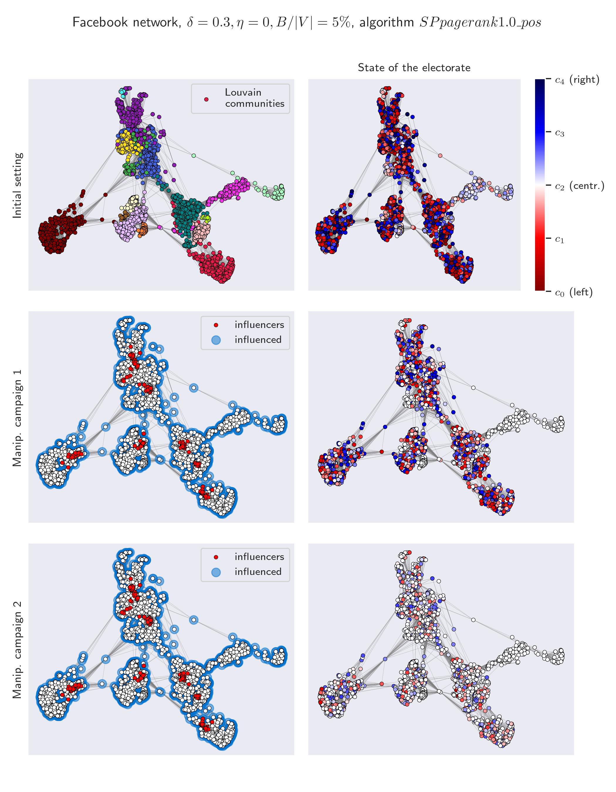
Figure 12: Facebook network. Evolution of the electorate after the first two manipulation campaigns.

Remember that nodes in the same community are tightly connected, while voters in different communities have lower chances of sharing information with each other. Hence, the algorithm should spend the budget to choose nodes in different communities to reach as many nodes as possible. However, since this is an election manipulation problem and not an influence maximization one, the algorithm searches for focused influence, discarding nodes that already vote for the target $c_{2}$ as they do not impact the margin of victory. All these considerations are actually internalized by algorithm SPpagerank1.0_pos, as revealed in Figure 12. The plots show the evolution of the electorate and the influencers chosen by the algorithm under the following conditions: ${\eta}=0$, $\delta=0.3$, $B/|V|=5\%$. Data concerns a single execution, as it would be in a real scenario: no averages were performed. The first row of the figure shows the Louvain communities as a reference and the initial state of the electorate (voters are coloured according to their political position on the spectrum; see the legend in the plot). It is clear that only a small subset of voters supports $c_{2}$, namely the communities on the right and some communities in the middle of the plot that are not clearly visible. The second row shows the influencers chosen by the algorithm and the state of the electorate after the first manipulation campaign. Interestingly, the influencers (represented as red dots) are distributed all over the communities to reach as many nodes as possible (represented as haloed, blue shadows). However, there is no influencer in the right part of the plot since such communities already supported $c_{2}$: choosing influencers in these communities would be a pointless waste of budget. The state of the electorate is represented by lighter colours which means that many voters changed their minds to support $c_{2}$. The same considerations apply to the second manipulation campaign (third row of the plot), after which much more nodes vote for the target candidate.

We finally evaluate the timing performances (numerical results are showed in Table 7).

	Round 1	Round 2	Round 3	Round 4	Round 5	Round 6	Round 7	Round 8	Round 9	Round 10
Alg
$PR1^{+}$	0.00242 s	0.00235 s	0.00228 s	0.00221 s	0.00214 s	0.00207 s	0.00202 s	0.00197 s	0.00194 s	0.00192 s
	$\pm$8.52e-05	$\pm$8.35e-05	$\pm$8.26e-05	$\pm$8.15e-05	$\pm$7.81e-05	$\pm$7.78e-05	$\pm$7.81e-05	$\pm$7.28e-05	$\pm$6.69e-05	$\pm$6e-05
$APX$	7.51 s	4.09 s	4.6 s	3.65 s	2.79 s	1.81 s	1.26 s	0.89 s	0.759 s	0.693 s
	$\pm$5.45	$\pm$2.37	$\pm$3.02	$\pm$2.5	$\pm$1.51	$\pm$0.886	$\pm$0.732	$\pm$0.672	$\pm$0.694	$\pm$0.715

Table 7: Simulation times of the fast heuristics and the approximation algorithms for 20 voters, ${\eta}=0$, 5 candidates. Each cell shows the average execution time and the standard deviation in seconds. $PR1^{+}$ and $APX$ respectively stand for SPpagerank1.0_pos and Approximation algorithm.

Execution times show that the approximation algorithm is thousands of times slower than the fast heuristic.

Finally, we tested the scalability of SPpagerank1.0_pos on networks up to 20000 nodes as described above (the numerical results of this experiment are shown in Table 8).

${\eta}$	$|V|=200$	$500$	$1000$	$2000$	$5000$	$10000$	$20000$
0	14743	7558	3842	1613	210	59	15
$\mathcal{N}(0;0.08)$	13204	6848	3495	1490	193	56	14
$\mathcal{N}(0;1.0)$	12693	6699	3443	1473	190	55	15

Table 8: Number of simulations of algorithm SPpagerank1.0_pos running on electorates of increasing sizes for three hours.

Interestingly, on a common PC, the algorithm can be executed 15 times in three hours on graphs of 20000 nodes. Since simulations require additional code to prepare the electoral setting and include 10 manipulation campaigns, the number of tests runnable in three hours is even higher. This means that a manipulator would not face any problem executing the proposed algorithm on large graphs.

The plot in Figure 13 analyzes the same results of Table 8 from a different perspective: it shows the average values of the total execution times, the execution times to compute the scores $z(v)$ of the nodes $v$, and the execution times to compute the weighted PageRank based on such scores. The plot considers only the first manipulation campaign since related execution times are surely not altered, unless unanimity in favour of the target candidate is reached (and thus the simulation is stopped).

Figure 13: Execution times of the algorithms SPpagerank1.0_pos in perfectly-single-peaked scenarios. The plot shows the average execution times to run the algorithm, compute the weights $z(\cdot)$, and compute PageRank values. The dashed line confirms that execution times grow according to a power law.

We can see that the cost of the algorithm is basically the one of PageRank, as the cost to compute $z(\cdot)$ is negligible. We know that search engines use it constantly on graphs of millions of nodes. Therefore, the algorithm is surely runnable on real problem instances involving millions of voters. The plot intentionally uses logarithmic scales for both the x-axis and the y-axis. In fact, it is clear that the execution times of the PageRank algorithm approximately follow a straight line proving that execution times grow according to a power law.

6 Conclusion

In this work we considered the problem of election manipulation through social influence when agents have single-peaked or nearly single-peaked preferences. For this purpose, we first propose a new manipulation model that intrinsically generates single-peaked preferences of the voters. We provided an algorithm with constant approximation guarantees whenever there is no agent that is more advantaged than the target candidate by a campaign in favour of the latter. We also provided an heuristics that has been proved to perform very well in simulations and to be computable very efficiently. These results highlight the huge risk of election manipulation in the single-peaked setting.

It would be desirable to further extend and deepen our analysis. Moreover, it would be interesting to design efficient and effective counter-measures against manipulation. Our analysis, by highlighting those aspects that simplify or complicate the manipulation, may be an useful starting point in this direction.

References

- [1] Abouei Mehrizi, M., Corò, F., Cruciani, E., D’Angelo, G.: Election control through social influence with voters’ uncertainty. Journal of Combinatorial Optimization 44(1), 635–669 (2022)
- [2] Allcott, H., Gentzkow, M.: Social media and fake news in the 2016 election. Journal of economic perspectives 31(2), 211–236 (2017)
- [3] Anshelevich, E., Bhardwaj, O., Elkind, E., Postl, J., Skowron, P.: Approximating optimal social choice under metric preferences. Artificial Intelligence 264, 27–51 (2018)
- [4] Auletta, V., Caragiannis, I., Ferraioli, D., Galdi, C., Persiano, G.: Minority becomes majority in social networks. In: WINE. pp. 74–88 (2015)
- [5] Auletta, V., Caragiannis, I., Ferraioli, D., Galdi, C., Persiano, G.: Information retention in heterogeneous majority dynamics. In: WINE. pp. 30–43 (2017)
- [6] Auletta, V., Caragiannis, I., Ferraioli, D., Galdi, C., Persiano, G.: Robustness in discrete preference games. In: AAMAS. pp. 1314–1322 (2017)
- [7] Auletta, V., Ferraioli, D., Fionda, V., Greco, G.: Maximizing the spread of an opinion when Tertium Datur Est. In: AAMAS. pp. 1207–1215 (2019)
- [8] Auletta, V., Ferraioli, D., Greco, G.: Reasoning about consensus when opinions diffuse through majority dynamics. In: IJCAI. pp. 49–55 (2018)
- [9] Auletta, V., Ferraioli, D., Greco, G.: On the effectiveness of social proof recommendations in markets with multiple products. In: ECAI. pp. 19–26 (2020)
- [10] Barabási, A.L., Albert, R.: Emergence of scaling in random networks. science 286(5439), 509–512 (1999)
- [11] Bartholdi, J.J., Tovey, C.A., Trick, M.A.: The computational difficulty of manipulating an election. Social Choice and Welfare 6, 227–241 (1989)
- [12] Bartholdi III, J.J., Orlin, J.B.: Single transferable vote resists strategic voting. Social Choice and Welfare 8(4), 341–354 (1991)
- [13] Bartholdi III, J.J., Tovey, C.A., Trick, M.A.: How hard is it to control an election? Mathematical and Computer Modelling 16(8-9), 27–40 (1992)
- [14] Borgs, C., Brautbar, M., Chayes, J., Lucier, B.: Maximizing social influence in nearly optimal time. In: SODA. pp. 946–957 (2014)
- [15] Brandt, F., Brill, M., Hemaspaandra, E., Hemaspaandra, L.A.: Bypassing combinatorial protections: Polynomial-time algorithms for single-peaked electorates. Journal of Artificial Intelligence Research 53, 439–496 (2015)
- [16] Bredereck, R., Elkind, E.: Manipulating opinion diffusion in social networks. In: Proceedings of the International Joint Conference on Artificial Intelligence (IJCAI). pp. 894–900 (2017)
- [17] Brin, S., Page, L.: The anatomy of a large-scale hypertextual web search engine. Computer networks and ISDN systems 30(1-7), 107–117 (1998)
- [18] Bruno, M., Lambiotte, R., Saracco, F.: Brexit and bots: characterizing the behaviour of automated accounts on twitter during the uk election. EPJ Data Science 11(1), 17 (2022)
- [19] Castiglioni, M., Ferraioli, D., Gatti, N., Landriani, G.: Election manipulation on social networks: seeding, edge removal, edge addition. Journal of Artificial Intelligence Research 71, 1049–1090 (2021)
- [20] Corò, F., Cruciani, E., D’Angelo, G., Ponziani, S.: Exploiting social influence to control elections based on positional scoring rules. Information and Computation 289, 104940 (2022)
- [21] Erdélyi, G., Lackner, M., Pfandler, A.: Computational aspects of nearly single-peaked electorates. Journal of Artificial Intelligence Research 58, 297–337 (2017)
- [22] Faliszewski, P., Gonen, R., Kouteckỳ, M., Talmon, N.: Opinion diffusion and campaigning on society graphs. Journal of Logic and Computation 32(6), 1162–1194 (2022)
- [23] Faliszewski, P., Hemaspaandra, E., Hemaspaandra, L.A.: How hard is bribery in elections? Journal of artificial intelligence research 35, 485–532 (2009)
- [24] Faliszewski, P., Hemaspaandra, E., Hemaspaandra, L.A.: The complexity of manipulative attacks in nearly single-peaked electorates. In: TARK. pp. 228–237 (2011)
- [25] Faliszewski, P., Hemaspaandra, E., Hemaspaandra, L.A., Rothe, J.: The shield that never was: Societies with single-peaked preferences are more open to manipulation and control. In: TARK. pp. 118–127 (2009)
- [26] Ferrara, E.: Disinformation and social bot operations in the run up to the 2017 french presidential election. First Monday (2017)
- [27] Giglietto, F., Iannelli, L., Rossi, L., Valeriani, A., Righetti, N., Carabini, F., Marino, G., Usai, S., Zurovac, E.: Mapping Italian news media political coverage in the lead-up to 2018 general election. Available at SSRN 3179930 0 (2018)
- [28] Habib, M., McDiarmid, C., Ramirez-Alfonsin, J., Reed, B.: Probabilistic methods for algorithmic discrete mathematics, vol. 16. Springer Science & Business Media (1998)
- [29] Kempe, D., Kleinberg, J., Tardos, É.: Maximizing the spread of influence through a social network. In: KDD. pp. 137–146 (2003)
- [30] Leskovec, J., Mcauley, J.: Learning to discover social circles in ego networks. Advances in neural information processing systems 25 (2012)
- [31] Leskovec, J., Sosič, R.: Snap: A general-purpose network analysis and graph-mining library. ACM Transactions on Intelligent Systems and Technology (TIST) 8(1), 1–20 (2016)
- [32] Matsa, K.E., Shearer, E.: News use across social media platforms 2018 (2018)
- [33] Sina, S., Hazon, N., Hassidim, A., Kraus, S.: Adapting the social network to affect elections. In: AAMAS. pp. 705–713 (2015)
- [34] Walsh, T.: Uncertainty in preference elicitation and aggregation. In: AAAI. p. 3–8 (2007)
- [35] Watts, D.J., Strogatz, S.H.: Collective dynamics of ‘small-world’ networks. Nature 393(6684), 440–442 (1998)
- [36] Wilder, B., Vorobeychik, Y.: Controlling elections through social influence. In: AAMAS. pp. 265–273 (2018)
- [37] Wu, J., Estornell, A., Kong, L., Vorobeychik, Y.: Manipulating elections by changing voter perceptions. In: IJCAI (2022)