Tree Drawings with Columns

Abstract

Our goal is to visualize an additional data dimension of a tree with multifaceted data through superimposition on vertical strips, which we call columns. Specifically, we extend upward drawings of unordered rooted trees where vertices have assigned heights by mapping each vertex to a column. Under an orthogonal drawing style and with every subtree within a column drawn planar, we consider different natural variants concerning the arrangement of subtrees within a column. We show that minimizing the number of crossings in such a drawing can be achieved in fixed-parameter tractable (FPT) time in the maximum vertex degree $\Delta$ for the most restrictive variant, while becoming NP-hard (even to approximate) already for a slightly relaxed variant. However, we provide an FPT algorithm in the number of crossings plus $\Delta$, and an FPT-approximation algorithm in $\Delta$ via a reduction to feedback arc set.

1 Introduction

Visualizations of trees have been used for centuries, as they provide valuable insights into the structural properties and visual representation of hierarchical relationships [14]. Over time, numerous approaches have been developed to create tree layouts that are both aesthetically pleasing and rich in information. These developments have extended beyond displaying the tree structure alone to also encompass different facets (dimensions) of the underlying data. As a result, researchers have explored various layout styles beyond layered node-link diagrams and even higher-dimensional representations [17, 16]. Hadlak, Schumann, and Schulz [10] introduced the term of a multifaceted graph for a graph with associated data that combines various facets (also called aspects or dimensions) such as spatial, temporal, and other data. An example of a multifaceted tree is a phylogenetic tree, that is, a rooted tree with labeled leaves where edge lengths represent genetic differences or time estimates by assigning heights to the vertices. In this paper, we introduce an extension of classical node-link drawings for rooted phylogenetic trees, where vertices are mapped to distinct vertical strips, referred to as columns. This accommodates not only an additional facet of the data but also introduces the possibility of crossings between edges, thus presenting us with new algorithmic challenges.

Motivation.

Our new drawing style is motivated by the visualization of transmission trees (i.e., the tree of who-infected-who in an infectious disease outbreak), which are phylogenetic trees that often have rich multifaceted data associated. In these visualizations, geographic regions associated with each case are commonly represented by coloring the vertex and its incoming edge [9]. However, there are scenarios where colors are not available or suitable. In such a case and in the context of a transmission tree, our alternative approach maps each, say, region or age group to a separate column (see Fig. 1). The interactive visualization platform Nextstrain [9] for tracking of pathogen evolution partially implements this with a feature that allows the mapping of the leaves to columns based on one facet. Yet, since they then leave out inner vertices and edges, the topology of the tree is lost. We hope that our approach enables users to quickly grasp group sizes and the number of edges (transmissions) between different groups.

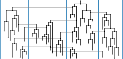
Figure 1: A binary column tree with four columns.

Related Work.

In visualization methods for so-called reconciliation trees [4, 2] and multi-species coalescent trees [6, 12], a guest tree $P$ is drawn inside a space-filling drawing of a host tree $H$. The edges of the host tree can thus closely resemble columns, though the nature of and relationship between $P$ and $H$ prohibit a direct mapping to column trees. Spatial data associated with a tree has also been visualized by juxtaposition for so-called phylogeographic trees [15, 13]. Betz et al. [1] investigated orthogonal drawings with column assignments, where each column is a single vertical line (i.e. analogous to a layer assignment).

Setting.

The input for our drawings consists of an unordered rooted tree $T$, where each vertex $v\in V(T)$ has an assigned height $h(v)$, and a surjective column mapping $c\colon V(T)\to[1,\ell]$ for some $\ell\geq 2$. Together, we call $\langle T,h,c\rangle$ a column tree. We mostly assume that the order of the columns is fixed (from 1 to $\ell$ left-to-right), but in a few places we also consider the case that it is variable. For an edge $uv$ in $T$, $u$ is the parent of $v$, and $v$ is the child of $u$. We call $u$ and $v$ the source and target (vertex) of $uv$, respectively. We call $uv$ an intra-edge if $c(u)=c(v)$ and an inter-edge otherwise. The degree of $u$ is the number of children of $u$.

Visualization of Column Trees.

We draw a column tree $\langle T,h,c\rangle$ with a rectangular cladogram style, that is, each edge is drawn orthogonally and (here) downward with respect to the root; hence we assume that $h$ corresponds to y-coordinates where the root has the maximum value and every parent vertex has a strictly greater value than its children. Each edge $uv$ has at most one bend such that the horizontal segment (if existent) has the y-coordinate of the parent vertex $u$. Each column $\gamma\in[1,\ell]$ is represented by a vertical strip $C_{\gamma}$ of variable width and a vertex $v$ with $c(v)=\gamma$ must be placed within $C_{\gamma}$. We need a few definitions to state further drawing conventions.

A column subtree is a maximal subtree within a column. Note that each column subtree (except the one containing the root of $T$) has an incoming inter-edge to its root and may have various outgoing inter-edges to column subtrees in other columns. The width of a column subtree at height $\eta$ is the number of edges of the column subtree intersected by the horizontal line at $\mathrm{y}=\eta$. We say that two column subtrees $A$ and $B$ interleave in a drawing of a column tree if there is a horizontal line that intersects first an edge of $A$, then one of $B$, and then again one of $A$ (or with $A$ and $B$ in reversed roles).

(a) V1 – subtree “stick” to column borders (13 crossings)

(b) V2 – non-interleaving subtrees (11 cr.)

(c) V3 – interleaving subtrees allowed (6 cr.)

Figure 2: The three variants for subtree arrangements.

In graph drawing, we usually forbid overlaps. Here, however, if a vertex has more than one child to, say, its right, then the horizontal segments of the edges to these children overlap. As we permit more than three children, we allow these overlaps and we do not count them as crossings. On the other hand, we do not want overlaps to occur between non-neighboring elements. Thus, we assume that each vertex $v$ being the source of an inter-edge has a unique height $h(v)$ as otherwise we cannot always avoid overlaps between an edge and a vertex and between two edges with distinct endpoints. Furthermore, we require that no two intra-edges cross. Hence, each column subtree is drawn planar and no two column subtrees intersect. However, since for inter-edges it is not always possible to avoid all edge crossings, we distinguish three drawing conventions concerning inter-edges and column subtree relations. These increasingly trade clarity of placement with the possibility to minimize the number of crossings (see Fig. 2):

1. No inter-edge $uv$ intersects an intra-edge in column $c(v)$.

2. No two column subtrees interleave.

3. Column subtrees may interleave.

We remark that V1 is based on the idea that going from top to bottom, the column subtree rooted at $v$ is greedily placed as soon as possible in $c(v)$. Thus, the subtrees “stick” to the column border closer to their root’s parent. Note that V1 implies V2 as interleaving a column subtree $B$ inside a column subtree $A$ requires that the incoming inter-edge of $B$ crosses an intra-edge of $A$.

Combinatorial Description.

We are less interested in the computation of x-coordinates but in the underlying algorithmic problems regarding the number of crossings. Hence, it suffices to describe a column tree drawing combinatorially in terms of what we call the subtree embeddings and the subtree arrangement of the drawing. The subtree embedding is determined by the order of the children of each vertex in the subtree. The subtree arrangement of a column represents the relative order between column subtrees that overlap vertically. From a computational perspective, one possible approach to specify the subtree arrangement is by storing, for each root vertex $v$ of a column subtree, which edges of which column subtrees lie horizontally to the left and to the right of $v$. This requires only linear space and all necessary information, e.g., for an algorithm that computes actual x-coordinates, can be recovered in linear time. A fixed column order, a subtree embedding of each column subtree, and a subtree arrangements of each column collectively form what we refer to as an embedding of a column tree $\langle T,h,c\rangle$.

Problem Definition.

An instance of the problem TreeColumns|V$i$, $i\in\{1,2,3\}$, is a column tree $\langle T,h,c\rangle$. The task is to find an embedding of $\langle T,h,c\rangle$ with the minimum total number of crossings among all possible embeddings of $T$ under the drawing convention V$i$. In the decision variant, an additional integer $k$ is given, and the task is to find a column embedding with at most $k$ crossings. If the column order is not fixed, we get another three problem versions.

We define three types of crossings. Consider an inter-edge $uv$ with $c(u)<~{}c(v)$. In any drawing, $uv$ spans over the columns $c(u)+1,\dots,c(v)-1$ and crosses always the same set of edges in these columns. We call the resulting crossings inter-column crossings, denoted by $k_{\mathsf{inter}}$. Within the column $c(u)$ [$c(v)$], $uv$ may cross edges of the column subtree of $u$ [$v$] and of other column subtrees. We call these crossings intra-subtree and intra-column crossings, denoted by $k_{\mathsf{subtree}}$ and $k_{\mathsf{column}}$, respectively. The total number of crossings is then $k=k_{\mathsf{subtree}}+k_{\mathsf{column}}+k_{\mathsf{inter}}$.

It would also be natural to seek an embedding or drawing with minimum width, yet this is known to be NP-hard even for a single phylogenetic tree [18].

Observe that for TreeColumns|V1 and V2, modifying the embedding of a single column subtree can only change the intra-subtree crossings. On the other hand, permuting the order of the column subtrees within a column can only change the intra-column crosssings. Finding a minimum-crossing embedding can thus be split into two tasks, namely, embedding the subtrees and finding a subtree arrangement. Furthermore, note that V1 mostly enforces a subtree arrangement since in general each column subtree is the left-/rightmost in its column at the height of its root. Only for column subtrees that are in the same column and whose roots share a parent, is the relative order not known. The main task for V1 is thus to find subtree embeddings. For V3, in contrast, the two tasks are intertwined since a minimum-crossing embedding may use locally suboptimal subtree embeddings (see Fig. 2(c)). We briefly discuss heuristics in Section 5.

Contribution.

We first give a fixed-parameter tractable (FPT) algorithm in the maximum vertex degree $\Delta$ for the subtree embedding task, the main task for V1 and a binary column tree (Section 2). We remark that the previously described applications usually use binary phylogenetic trees. This makes our algorithm, which uses a sweep line to determine the crossing-minimum child order at each vertex, a practically relevant polynomial-time algorithm. On the other hand, if we have a large vertex degree, minimizing the number of crossings is NP-hard, even to approximate, for all variants (Section 3). This holds true for the less restrictive variants V2 and V3 even for binary trees. Leveraging a close relation between the task of finding a column subtree arrangement and the feedback arc set (FAS) problem, we devise for V2 an FPT algorithm in the number of crossings $k$ plus $\Delta$ and an FPT-approximation algorithm in $\Delta$ (Section 4). However, for the most general variant V3, the tasks of embedding the column subtrees and arranging them cannot be considered separately, and hence we only suggest heuristics to address this challenge (Section 5).

2 Algorithm for Subtree Embedding

In this section, we describe how to find an optimal subtree embedding for a single column subtree. The algorithm has an FPT running time in the maximum vertex degree $\Delta$ making it a polynomial-time algorithm for bounded-degree trees like binary trees, ternary trees, etc.

Our algorithm is based on the following observation, described here for a binary column subtree $S$. Fix an embedding for $S$, i.e., the child order for each vertex. Consider an inter-edge $e=vw$ with $c(w)<c(v)$. Let $u$ be a vertex of the path from the parent of $v$ to the root of $B$. Observe that if $v$ is in the left subtree of $u$, then $e$ does not intersect the right subtree of $u$. Yet, if $v$ is in the right subtree of $u$, then $e$ intersects the left subtree of $u$ (if it extends vertically beyond $h(v)$). On the other hand, if $u$ is not on the path to the root, then the child order of $u$ has no effect on whether $e$ intersects its subtrees. Thus, to find an optimal child order of a vertex, it suffices to consider the directions (left/right) towards which the inter-edges of its descendants extend. Our algorithm is illustrated in Fig. 3.

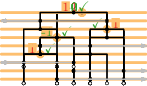
(a) Initial embedding and first inter-edge.

(b) The second inter-edge.

(c) The third inter-edge.

(d) Keeping a child order to avoid one crossing.

(e) The fourth inter-edge.

(f) Keeping a child order to avoid one crossing.

(g) Changing a child order to avoid one crossing.

(h) The fifth inter-edge.

(i) Changing the child order of the root to avoid one crossing.

Figure 3: Steps of the sweep-line algorithm to find, for a given (here, binary) column subtree, a subtree embedding with the minimum number of intra-subtree crossings. A number at a vertex $v$ reflects the count of crossings for the two possible permutations of $v$ (positive number $\Leftrightarrow$ more crossings if $v$’s child order is kept). In steps considering inter-edges, affected ancestor vertices are marked orange.

Lemma 1

For an $n$-vertex column subtree $S$ with maximum degree $\Delta$ and $t$ inter-edges, a minimum-crossing subtree embedding of $S$ can be computed in $\mathcal{O}(\Delta!\Delta tn+n\log n)$ time.

Proof

In a bottom-to-top sweep-line approach over $S$, we apply the following greedy-permuting strategy that finds, for each vertex, the child order that causes the fewest crossings. To this end, first sort the vertices of $S$ by ascending height in $\mathcal{O}(n\log n)$ time. Also, each inner vertex $v$ with $d_{v}$ ($d_{v}\leq\Delta$) children in $S$ has $d_{v}!$ counters to store for each of the $d_{v}!$ possible child orders (of its children in $S$) the computed number of crossings induced by that order (as described below). Initially, all counter are set to zero.

Having started at the bottom, let $v$ be the next encountered vertex. First, process each inter-edge $e$ whose source is $v$. Let $u$ be a vertex on the path $P$ from the parent of $v$ to the root. Let $T_{v}$ be the subtree rooted at a child of $u$ that contains $v$. Compute for each subtree $T$ rooted at a child of $u$ (except for $T_{v}$) the width at $h(v)$ as follows.

Initialize a counter for the width of $T$ at $h(v)$ with zero. Traverse $T$ and whenever we encounter an edge of $T$ that has one endpoint above and the other endpoint on or below $h(v)$, we increment that counter. Hence, we can determine the width of $T$ at $h(v)$ in $\mathcal{O}(n_{T})$ time, where $n_{T}$ is the number of vertices in $T$, and we can determine the width of all subtrees rooted at children of vertices from $P$ in $\mathcal{O}(n)$ time.

Recall that $u$ has $d_{u}!$ (with $d_{u}\leq\Delta$) counters for its $d_{u}!$ possible child orders. For each such child order, add, if $e$ goes to the left [right], the width at $h(v)$ of all subtrees rooted at children of $u$ that are left [right] of $T_{v}$ to the corresponding counter. Note that the resulting number is exactly the number of intra-subtree crossings induced by $e$, as our observation still holds for the general case because the number of intra-subtree crossings induced by $e$ only depends on the child orders of the vertices of $P$. Of course, as the numbers are independent of other inter-edges, we can add up these numbers in our child order counters. Updating these counters for a vertex $u$ on $P$ takes $\mathcal{O}(d_{u}!d_{u})\subseteq\mathcal{O}(\Delta!\Delta)$ time. Since the length of $P$ can be linear, we can handle $e$ in $\mathcal{O}(\Delta!\Delta n)$ time.

Second, since the counters of $v$ only depend on the already processed inter-edges below $v$, pick the child order of $v$ with the lowest counter for $v$.

In total, this sweeping phase of the algorithm runs in $\mathcal{O}(\Delta!\Delta tn)$ time, where $t$ is the number of inter-edges. This is because, although the sweep-line algorithm has $\Theta(n)$ event points (the vertices of $S$), we apply the previously described $\mathcal{O}(\Delta!\Delta n)$-time subroutine only if we encounter an inter-edge.

Note that for Lemma 1, if $t=0$, any embedding is crossing free, and if $\Delta$ is constant, the running time is at most quadratic in $n$.

To solve an instance of TreeColumns|V1, we first apply Lemma 1 to each column subtree separately. Then for each vertex with multiple outgoing inter-edges to the same column, we try all possible orders for the respective column subtrees and keep the best. Hence, we get the following result.

Theorem 2.1

TreeColumns|V1 is fixed-parameter tractable in $\Delta$. More precisely, given an instance $\langle T,h,c\rangle$ with $n$ vertices and maximum vertex degree $\Delta$, there is an algorithm computing an embedding of $\langle T,h,c\rangle$ with the minimum number of crossings in $\mathcal{O}(\Delta!\Delta n^{2})$ time.

3 NP-Hardness and APX-Hardness

In this section, we show that TreeColumns becomes NP-hard (even to approximate) when finding a subtree arrangement is non-trivial or if we have large vertex degrees. We use a reduction from the (unweighted) Feedback Arc Set (FAS) problem, where we are given a digraph $G$ and the task is to find a minimum-size set of edges that if removed make $G$ acyclic. We assume, without loss of generality, that $G$ is biconnected. FAS is one of Karp’s original 21 NP-complete problems [11]. It is also NP-hard to approximate within a factor less than $1.3606$ [5] and, presuming the unique games conjecture, even within any constant factor [8].

Theorem 3.1

The TreeColumns problem is NP-complete for both fixed and variable column orders already for two columns under V1 if the degree is unbounded, and under V2 and V3 even for a binary column tree. Moreover, it is NP-hard to approximate within a factor of $1.3606-\varepsilon$ for any $\varepsilon>0$, and NP-hard to approximate within any constant factor presuming the unique games conjecture.

Proof

The problem is in NP, since given an embedding for a column tree, it is straightforward to check whether it has at most $k$ crossings in polynomial time.

To prove NP-hardness (of approximation), we use a reduction from FAS. Let $G$ be an instance of FAS; let $n=\lvert V(G)\rvert$ and $m=\lvert E(G)\rvert$, and fix an arbitrary vertex order via the indices, so $V(G)=\{v_{1},\ldots,v_{n}\}$, and an arbitrary edge order. We construct a column tree $\langle T,h,c\rangle$ such that there is a bijection between vertex orders of $G$ (where each vertex order implies a solution set for the FAS problem) and solutions of $\langle T,h,c\rangle$, whose number of crossings depends on the size of the FAS solution and vice versa. We show this first for V1 with unbounded degree; see Fig. 4.

Give $T$ two columns and, assuming for now that their order is fixed, call them left and right column. The total height of $T$ is $a=3(m+1)$. The root column subtree of $T$ is in the left column, and has a single inner vertex $v$ at $a-1$. For each $v_{i}\in V(G)$, there is an inter-edge from $v$ to a column subtree $T_{i}$, the vertex gadget of $v_{i}$, in the right column. The idea is that a subtree arrangement of $\{T_{1},\dots,T_{n}\}$ corresponds to a topological order of $G\setminus S$ where each edge whose edge gadget induces a large number of crossings is in the FAS solution set $S$.

Vertex Gadget.

The subtree $T_{i}$ has a backbone path on $\deg(v_{i})+1$ vertices with its leaf at height 0. Attached to the backbone of $T_{i}$, there are inter-edges and subtrees depending on the edges incident to $v_{i}$. We describe them next.

Edge Gadget.

The edge gadget for an edge $v_{i}v_{j}\in E(G)$ consists of an inter-edge $e_{i,j}$ to the left column attached to the backbone of $T_{i}$ and of a star $S_{i,j}$ with $n^{3}$ leaves attached to the backbone of $T_{j}$. Both are contained in a horizontal strip of height three. So if $v_{i}v_{j}$ is, say, the $t$-th edge, then we use the heights between $b=a-3t$ to $b-2$. The root of $S_{i,j}$ is at height $b$ and the leaves of $S_{i,j}$ are at height $b-2$. The source and the target of $e_{i,j}$ are at heights $b-1$ and $b-2$, respectively. Note that every $T_{i}$ (on its own) can always be drawn planar.

(a) A FAS instance on three edges.

(b) In the corresponding column subtree for V1, each edge gadget occupies a horizontal strip and we need to find a subtree arrangement of the vertex gadgets (grey background).

Figure 4: Reduction of a FAS instance to a TreeColumns instance.

Analysis of Crossings.

Note that, for each $v_{i}v_{j}\in E(G)$, the inter-edge $e_{i,j}$ induces at most $n-1$ crossings with the backbones of $\{T_{1},\dots,T_{n}\}$ independent of the subtree arrangement. With $m\leq n(n-1)/2$, there can thus be at most $n(n-1)/2\cdot(n-1)=n^{3}/2-n^{2}+n/2$ crossings that do not involve a star subtree. Now, if $T_{i}$ is to the left of $T_{j}$, then $e_{i,j}$ does not intersect $S_{i,j}$. On the other hand, if $T_{i}$ is to the right of $T_{j}$, then $e_{i,j}$ intersects $S_{i,j}$, which causes $n^{3}$ crossings. So, for a subtree arrangement with $s$ edge gadgets causing crossings, the embedding of $T$ contains $sn^{3}$ plus at most $rn^{3}$ crossings, where $r=1/2-1/n+1/(2n^{2})\leq 1$.

Bijection of Vertex Orders and Subtree Arrangements.

As each columns subtree $T_{i}$ ($i\in\{1,\dots,n\}$) corresponds to vertex $v_{i}$ of $G$, each subtree arrangement of $\langle T,h,c\rangle$ implies exactly one vertex order of $G$ and vice versa. A vertex order $\Pi$ of $G$, in turn, implies the FAS solution set containing all edges whose target precedes its source in $\Pi$. In the other direction, for a FAS solution set $S$, we find a corresponding vertex order by computing a topological order of $G\setminus S$.

Consequently, a subtree arrangement of $\langle T,h,c\rangle$ whose number $k$ of crossings lies in $[sn^{3},(s+r)n^{3}]$ implies a FAS solution of size $s$ and vice versa. In particular, a minimum-size FAS solution of size $s^{*}$ corresponds to an optimal subtree arrangement with $k_{\min}=(s^{*}+r^{*})n^{3}$ crossings, where $0\leq r^{*}\leq r\leq 1$.

Hardness of Approximation.

If it is NP-hard to approximate FAS by a factor less than $\alpha$, then it is NP-hard to approximate TreeColumns|V1 by a factor less than $\beta$ due to the previous bijection, where $\beta$ can be bounded as follows.

$$\beta\cdot k_{\min}=\beta\cdot(s^{*}+r^{*})n^{3}\geq\alpha s^{*}n^{3}\quad\Leftrightarrow\quad\beta\geq\frac{\alpha s^{*}}{s^{*}+r^{*}}=\alpha-\frac{\alpha r^{*}}{s^{*}+r^{*}}$$

Since $s^{*}$ is unbounded, $\alpha r^{*}/(s^{*}+r^{*})$ can be arbitrarily close to zero. Hence, it is NP-hard to approximate TreeColumns|V1 with unbounded maximum degree within any factor $\alpha-\varepsilon$ for any $\varepsilon>0$.

Figure 5: Reduction for V2 & V3 with binary trees.

Other Variants.

For a variable column order, note that, for our bijection, the vertex order is the same but mirrored if we swap the left and right column.

For a binary column tree under V2 and V3, we let the sources of the inter-edges in the root column subtree, which have as targets the roots of the $T_{i}$, form a path in the root column subtree; see Fig. 5. These edges can form at most $n^{2}$ pairwise crossings, which changes $r$ and $r^{*}$ only slightly and has thus no effect on our bijection. Similarly, the star subtrees can simply be substituted with binary subtrees where all inner vertices have a height between $b$ and $b-1$. Also note that the $T_{i}$ cannot interleave since they span from above the first edge gadgets all the way to the bottom.

Note that in the proof of Theorem 3.1, the variant with binary columns trees does not work under V1 (see Fig. 5), since then it would no longer be possible to permute the $T_{i}$; there would only be one possible subtree arrangement.

4 Algorithms for Subtree Arrangement

In the previous section, we have seen that TreeColumns|V2 is NP-hard, even to approximate, by reduction from FAS. Next, we show that we can also go the other way around and reduce TreeColumns|V2 to FAS to obtain an FPT algorithm in the number of crossings and the maximum vertex degree $\Delta$, and to obtain an FPT-approximation algorithm in $\Delta$.

Integer-Weighted Feedback Arc Set.

As an intermediate step in our reduction, we use the Integer-Weighted Feedback Arc Set (IFAS) problem which is defined for a digraph $G$ as FAS but with the additional property that each edge $e$ has a positive integer weight $w(e)$, $w\colon E(G)\rightarrow\mathbb{N}$, and the objective is to find a minimum-weight set of edges whose removal results in an acyclic graph. Clearly, IFAS is a generalization of FAS because FAS is IFAS with unit weights. However, an instance $\langle G,w\rangle$ of IFAS can also straightforwardly be expressed as an instance $G^{\prime}$ of FAS: Obtain $G^{\prime}$ from $G$ by substituting each edge $uv$ with $w(uv)$ length-two directed paths from $u$ to $v$. For an illustration, see Fig. 6.

(a) Input IFAS instance $\langle G,w\rangle$ with minimum-weight solution $S=\{e\}$.

(b) Output FAS instance $G^{\prime}$ with minimum-size solution $S^{\prime}=\{e_{1},e_{2}\}$.

Figure 6: Reduction of an IFAS instance to a FAS instance.

Lemma 2

We can reduce an instance $\langle G,w\rangle$ of IFAS with $m$ edges and maximum weight $w_{\max}$ to an instance $G^{\prime}$ of FAS in time $\mathcal{O}(mw_{\max})$ such that

• $G^{\prime}$ has size in $\mathcal{O}(mw_{\max})$,

• the size of a minimum-size solution of $G^{\prime}$ equals the weight of a minimum-weight solution of $\langle G,w\rangle$, and

• we can transform a solution of $G^{\prime}$ with size $s$ in $\mathcal{O}(s)$ time to a solution of $G$ with weight at most $s$.

Proof

Note that, by construction, $G^{\prime}$ has size in $\mathcal{O}(mw_{\max})$ and can be construct in $\mathcal{O}(mw_{\max})$ time.

Consider any minimum-weight solution $S$ of $\langle G,w\rangle$ with total weight $s$. We can transform it to a solution $S^{\prime}$ of $G^{\prime}$ of size $s$ by removing, for each edge $uv$ of $S^{\prime}$, all first edges of the $w(uv)$ length-two paths representing $uv$ in $G^{\prime}$. If $G^{\prime}\setminus S^{\prime}$ had a cycle $C$, then a cycle half the length of $C$ would also occur in $G\setminus S$.

For any solution $S^{\prime}$ of $G^{\prime}$ with size $s$, there is also a solution $S$ of $\langle G,w\rangle$ with total weight at most $s$: For an edge $uv$ in $G$, consider the $w(uv)$ length-two paths representing $uv$ in $G^{\prime}$. If $S^{\prime}$ contains at least one edge of every such path, we add the edge $uv$ to the solution $S$. Clearly, the weight of $S$ is at most the number of edges in $S^{\prime}$. Suppose for a contradiction that there is a cycle $C$ in $G\setminus S$. Then, there would also be a cycle in $G^{\prime}\setminus S$ because for every edge of $C$, there is at least one length-two path left in $G^{\prime}$ after removing $S^{\prime}$.

Reduction to Feedback Arc Set.

Next, we show that we can express every instance of TreeColumns|V2 as an instance of IFAS. Note, however, that we have split the problem into the tasks of embedding the subtrees and finding a subtree arrangement. Here, we are only concerned with finding a subtree arrangement for every column, and we assume that we separately solve the problem of embedding every column subtree, e.g., by employing the algorithm from Lemma 1.

Lemma 3

We can reduce an instance $\langle T,h,c\rangle$ of TreeColumns|V2 on $n$ vertices to an instance $\langle G,w\rangle$ of IFAS in time $\mathcal{O}(n^{2})$ such that

• $G$ has size in $\mathcal{O}(n^{2})$ and maximum weight $w_{\max}\in\mathcal{O}(n^{2})$,

• the number of intra-column crossings in a minimum-crossing solution of $\langle T,h,c\rangle$ equals the weight of a minimum-weight solution of $\langle G,w\rangle$ plus $t$ where $t$ is some integer in $\mathcal{O}(n^{2})$ depending only on $\langle T,h,c\rangle$, and

• we can transform a solution of $\langle G,w\rangle$ with weight $s$ in $\mathcal{O}(n^{2})$ time to a solution of $\langle T,h,c\rangle$ with at most $s+t$ intra-column crossings.

(a) Possible permutation $\Pi$ of the subtrees.

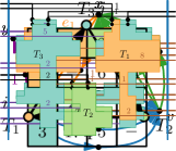
(b) Reverse permutation of $\Pi$.

(c) Table of pairwise intra-column crossings $k_{ij}$ occurring if subtree $T_{i}$ is placed to the left of subtree $T_{j}$.

(d) Resulting IFAS instance where the difference $k_{ij}-k_{ji}$ determines the direction and the weight of an edge.

Figure 7: Reduction of an TreeColumns|V2 instance to an IFAS instance.

Proof

To each column in $c$, we apply the following reduction; see Fig. 7. Let $T_{1},\dots,T_{r}$ be the set of column subtrees of $c$. For each pair $T_{i},T_{j}$ of subtrees ($i,j\in\{1,\dots,r\},i\neq j$), we consider the number of intra-column crossings where only edges with an endpoint in $T_{i}$ and $T_{j}$ are involved – once if $T_{i}$ is placed to the left of $T_{j}$ and once if $T_{j}$ is placed to the left of $T_{i}$; see Figs. 7(a) and 7(b). We let these numbers be $k_{ij}$ and $k_{ji}$, respectively; see Fig. 7(c). We then construct an IFAS instance $\langle G,w\rangle$ where $G$ has a vertex for every column subtree. For each pair $T_{i},T_{j}$, $G$ has the edge $T_{i}T_{j}$ if $k_{ij}-k_{ji}<0$, or $G$ has the edge $T_{j}T_{i}$ if $k_{ij}-k_{ji}>0$, or there is no edge between $T_{i}$ and $T_{j}$ otherwise. The weight of each edge is $\lvert k_{ij}-k_{ji}\rvert$. So we have an edge in the direction where the left-to-right order yields fewer intra-column crossings, and no edge, if the number of intra-column crossings is the same, no matter their order.

Note that instead of considering each column separately, we can also think of $G$ as a single graph having at least one connected component for each column.

Implementation and Running Time.

For counting the number of crossings between pairs of subtrees, we initialize $\mathcal{O}(r^{2})$ variables with zero. Then, we use a horizontal sweep line traversing all trees in parallel top-down while maintaining the current widths of $T_{1},\dots,T_{r}$ in variables $b_{1},\dots b_{r}$. Our event points are the heights of the vertices (given by $h$) and the heights of the parents of the subtree roots (where we have the horizontal segment of an edge entering the column).

Whenever we encounter an inter-edge $uv$, we update the crossing variables. More precisely, if $u\in T_{i}$ for some $i\in\{1,\dots,r\}$, we consider each $j\in\{1,\dots,r\}\setminus\{i\}$ and we set $k_{ji}+$$=b_{j}$ if $v$ is in a column on the left, and, symmetrically, we set $k_{ij}+$$=b_{j}$ if $v$ is in a column on the right.

The running time of this approach is $\mathcal{O}(r(n_{\mathrm{column}}+m_{\mathrm{column}}))$ per column where $n_{\mathrm{column}}$ and $m_{\mathrm{column}}$ are the numbers of vertices and edges in the column, respectively. Over all columns, this can be accomplished in $\mathcal{O}(n^{2})$ time.

Size of the Instance.

The resulting graph $G$ has $\mathcal{O}(n)$ vertices and $\mathcal{O}(n^{2})$ edges as we may have an edge for every pair of subtrees in a column and we may have a linear number of column subtrees. The maximum weight $w_{\max}$ in $w$ is in $\mathcal{O}(n^{2})$ since we have $\mathcal{O}(n)$ inter-edges and the maximum width of a tree is in $\mathcal{O}(n)$.

Comparison of Optima.

For each column $\gamma\in\{1,\dots,\ell\}$, we have the following lower bound $L_{\gamma}$ on the number $k_{\textrm{column}}^{\gamma}$ of intra-column crossings:

$$L_{\gamma}=\sum_{i=1}^{r-1}\sum_{j=i+1}^{r}\min\{k_{ij},k_{ji}\}\leq k_{\textrm{column}}^{\gamma}.$$

Now consider a minimum-crossing solution of $\langle T,h,c\rangle$. In column $\gamma$, the column subtrees have a specific order, which we can associate with a permutation $\Pi^{*}$ of the column subtrees. For simplicity, we rename the column subtrees as $T_{1},\dots,T_{r}$ according to $\Pi^{*}$. Then, the number of intra-column crossings is

$$k_{\textrm{column}}^{\gamma}=\sum_{i=1}^{r-1}\sum_{j=i+1}^{r}k_{ij}.$$

Because it is a minimum-crossing solution, the number $\delta_{\gamma}$ of additional crossings (i.e., the deviation of $k_{\textrm{column}}^{\gamma}$ from $L_{\gamma}$) due to “unfavorably” ordered pairs of subtrees is minimized. We can express $\delta_{\gamma}$ in terms of all $k_{ij}$ by

$$\delta_{\gamma}=k_{\textrm{column}}^{\gamma}-L_{\gamma}=\sum_{i\neq j,k_{ij}>k_{ji}}k_{ij}-k_{ji}.$$

Now consider a minimum-weight solution $S$ of $\langle G,w\rangle$ with weight $s$. After removing $S$ from $G$, we have an acyclic graph for which we can find a topological order $\Pi$ of its vertices, which in turn correspond to the column subtrees in $\langle T,h,c\rangle$. Again, we rename these subtrees as $T_{1},\dots,T_{r}$ according to $\Pi$. If we arrange $G$ linearly according to $\Pi$, only the edges of $S$ point backward and, by definition of the edge directions, for exactly these edges $k_{ij}>k_{ji}$ holds. The sum

$$s_{\gamma}=\sum_{i\neq j,k_{ij}>k_{ji}}k_{ij}-k_{ji}$$

of weights in $S$ whose vertices represent pairs of column subtrees in $\gamma$ is minimized because $G$ has independent components for all columns in $c$. Therefore, $s_{\gamma}=\delta_{\gamma}$. Over all columns $\{1,\dots,\ell\}$, we set $t=\sum_{i=1}^{\ell}L_{i}$, we have $s=\sum_{i=1}^{\ell}s_{i}$, and we conclude

$$k_{\textsf{column}}=\sum_{i=1}^{\ell}k_{\textrm{column}}^{i}=\sum_{i=1}^{\ell}(L_{i}+\delta_{i})=\sum_{i=1}^{\ell}(L_{i}+s_{i})=s+t.$$

Note that $t\in\mathcal{O}(n^{2})$ as we have $\mathcal{O}(n^{2})$ pairs of edges, which cross at most once.

Transforming a Solution Back.

Similarly, we can find for any solution $S$ of $\langle G,w\rangle$ with size $s$ a topological order, which corresponds to a subtree arrangement in $\langle T,h,c\rangle$. There, together with the $t$ unavoidable crossings, we have at most $s$ additional crossings due to “unfavorably” ordered pairs. We can find the topological order in linear time in the size of $G$, which is in $\mathcal{O}(n^{2})$.

When we combine Lemmas 3 and 2, we obtain Corollary 1.

Corollary 1

We can reduce an instance $\langle T,h,c\rangle$ of TreeColumns|V2 on $n$ vertices to an instance $G$ of FAS in time $\mathcal{O}(n^{4})$ such that

• $G$ has size in $\mathcal{O}(n^{4})$,

• the number of intra-column crossings in a minimum-crossing solution of $\langle T,h,c\rangle$ equals the size of a minimum-size solution of $G$ plus $t$ where $t$ is some integer in $\mathcal{O}(n^{2})$ depending only on $\langle T,h,c\rangle$, and

• we can transform a solution of $G$ with size $s$ in $\mathcal{O}(n^{2})$ time to a solution of $\langle T,h,c\rangle$ with $s+t$ crossings.

Fixed-Parameter Tractable Algorithm.

For TreeColumns|V2, one of the most natural parameters is the number of crossings, which is also the objective value. With our reduction to FAS at hand, it is easy to show that TreeColumns|V2 is fixed-parameter tractable (FPT) in this parameter for bounded-degree column trees. This follows from the fact that FAS is FPT in its natural parameter (the solution size) as first shown by Chen, Liu, Lu, O’Sullivan, and Razgon [3].

Theorem 4.1

TreeColumns|V2 is fixed-parameter tractable in the number $k$ of crossings plus $\Delta$. More precisely, given an instance $\langle T,h,c\rangle$ with $n$ vertices and maximum vertex degree $\Delta$, there is an algorithm computing an embedding with the minimum number $k$ of crossings in $\mathcal{O}(\Delta!\Delta n^{2}+n^{16}4^{k}k^{3}k!)$ time.

Proof

First, we find an embedding of every column subtree inducing the minimum number of intra-subtree crossings in $\mathcal{O}(\Delta!\Delta n^{2})$ time (see Lemma 1).

Employing Corollary 1, we reduce $\langle T,h,c\rangle$ in time $\mathcal{O}(n^{4})$ to an instance $G$ of FAS of size $\mathcal{O}(n^{4})$. We compute a minimum-size solution $S$ for the FAS instance $G$ in time $\mathcal{O}((n^{4})^{4}4^{s}s^{3}s!)$ where $s=|S|$ [3]. In $\mathcal{O}(n^{2})$ time, we use $S$ to compute a subtree arrangement of $\langle T,h,c\rangle$. We return the resulting embedding.

This solution has $k=k_{\mathsf{subtree}}+k_{\mathsf{column}}+k_{\mathsf{inter}}$ crossings, where $k_{\mathsf{subtree}}$ and $k_{\mathsf{column}}$ are minimum due to Lemma 1 and Corollary 1, respectively. As $k_{\mathsf{inter}}$ is always the same, the resulting embedding has the minimum number of crossings.

Overall, this algorithm runs in $\mathcal{O}(\Delta!\Delta n^{2}+n^{4}+(n^{4})^{4}4^{s}s^{3}s!+n^{2})$ time. Since $s\leq k$, this is an FPT algorithm in $k+\Delta$.

Approximation Algorithm.

Similar to our FPT result, we can use any approximation algorithm for FAS to approximate TreeColumns|V2. It is an unresolved problem whether FAS admits a constant-factor approximation. In case such an approximation is found, this immediately propagates to TreeColumns|V2. Currently, we can employ the best known approximation algorithm of FAS due to Even, Naor, Schieber, and Sudan [7], which has an approximation factor of $\mathcal{O}(\log n^{\prime}\log\log n^{\prime})$, where $n^{\prime}$ is the number of vertices in the FAS instance. We remark that this algorithm involves solving a linear program and the authors do not write much about precise running time bounds, which we also avoid here.

Theorem 4.2

There is an approximation algorithm that, for a given instance $\langle T,h,c\rangle$ of TreeColumns|V2 with $n$ vertices and maximum degree $\Delta$, computes in $\mathcal{O}(\mathsf{poly}(n)\cdot\Delta!\Delta)$ time an embedding where the number of crossings is at most $\mathcal{O}(\log n\log\log n)$ times the minimum number of crossings.

Proof

First, we find an embedding of every column subtree inducing the minimum number of intra-subtree crossings in $\mathcal{O}(\Delta!\Delta n^{2})$ time (see Lemma 1).

Employing Corollary 1, we reduce $\langle T,h,c\rangle$ in polynomial time to an instance $G$ of FAS of size $\mathcal{O}(n^{4})$. Using the algorithm by Even et al. [7], we compute an approximate solution $S$ for the FAS instance $G$ where $|S|$ is greater than an optimal solution by at most a factor in $\mathcal{O}(\log n^{4}\log\log n^{4})=\mathcal{O}(\log n\log\log n)$. From $S$, we compute a subtree arrangement in polynomial time. We return the resulting embedding.

In this embedding, the number of inter-column crossings and the number of intra-subtree crossings is minimum, and only the number of intra-column crossings is approximated. Therefore, the approximation factor of $\mathcal{O}(\log n\log\log n)$ holds for the total number $k$ of crossings as well.

5 Heuristic Approaches for Harder Versions

Here, we briefly discuss how to approach harder variants of the TreeColumns problem, specifically under V3 or with a variable column order.

TreeColumns|V3.

Recall that, compared to V2, in V3 column subtrees may interleave within a column. By Theorem 3.1, the TreeColumns|V3 problem is NP-hard even for binary column trees and the proof does not require interleaving. However, as shown in Fig. 2, interleaving can help to reduce the number of crossings. So while the two tasks of subtree embedding and subtree arrangement cannot be considered separately, it is still natural to try this as a heuristic.

A greedy approach for TreeColumns|V3 could work as follows. First, find an optimal embedding for each column subtree using the algorithm from Lemma 1. Second, for each column, sort the column trees in descending order based on their root heights. Then, in this order, add one column tree at a time at the horizontal position where it induces the smallest number of new crossings. We leave the details on how to find this position open for now. And while we think that this strategy can work well in practice, we want to point out that, in general, it can cause linearly more crossings than the optimum: The two column trees in Fig. 8 can be drawn without intra-subtree crossings (Figs. 8(a), 8(b) and 8(c)), yet even with interleaving we get a linear number of (intra-column) crossings. However, at the cost of two intra-subtree crossings, we can reduce the total number of crossings to four; see Fig. 8(d).

(a)

(b)

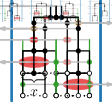
(c)

(d)

Figure 8: With $x\approx n/2$, computing optimal subtree embeddings first (a–c) can cause linearly more crossings than using a non-optimal subtree embedding and interleaving (d). (Each of the schematic subtrees has $x$ leaves.)

Variable Column Order.

In many cases in practice, the column order can be assumed to be fixed as there is, for example, a natural order for age groups and even for geographic regions of a country, there might be a preferred or standard ordering. Let us nonetheless assume now that the column order is not fixed but variable. We want to remark that we can still get the same results from Section 4 (under V2) if we add another parametric dependence on the number $\ell$ of columns; we can try all $\ell!$ permutations of the columns and apply these algorithms to each of them. While we can expect $\ell$ in practice to be low, this becomes in general, of course, quickly infeasible. Alternatively, we might try to find a column order that minimizes the number of inter-column crossings, for example with a greedy algorithm. The three different tasks, namely, finding a column order, subtree embeddings, and subtree arrangement, would thus focus on the three different crossings types.

References

- [1] Gregor Betz, Andreas Gemsa, Christof Mathies, Ignaz Rutter, and Dorothea Wagner. Column-based graph layouts. Journal of Graph Algorithms and Applications, 18(5):677–708, 2014. doi:10.7155/jgaa.00341.
- [2] Tiziana Calamoneri, Valentino Di Donato, Diego Mariottini, and Maurizio Patrignani. Visualizing co-phylogenetic reconciliations. Theoretical Computer Science, 815:228–245, 2020. doi:10.1016/j.tcs.2019.12.024.
- [3] Jianer Chen, Yang Liu, Songjian Lu, Barry O’Sullivan, and Igor Razgon. A fixed-parameter algorithm for the directed feedback vertex set problem. Journal of the ACM, 55(5):21:1–21:19, 2008. doi:10.1145/1374376.1374404.
- [4] François Chevenet, Jean-Philippe Doyon, Céline Scornavacca, Edwin Jacox, Emmanuelle Jousselin, and Vincent Berry. SylvX: A viewer for phylogenetic tree reconciliations. Bioinformatics, 32(4):608–610, 2016. doi:10.1093/bioinformatics/btv625.
- [5] Irit Dinur and Samuel Safra. On the hardness of approximating vertex cover. Annals of Mathematics, 162(1):439–485, 2005. doi:10.4007/annals.2005.162.439.
- [6] Jordan Douglas. UglyTrees: A browser-based multispecies coalescent tree visualizer. Bioinformatics, 07 2020. doi:10.1093/bioinformatics/btaa679.
- [7] Guy Even, Joseph Naor, Baruch Schieber, and Madhu Sudan. Approximating minimum feedback sets and multicuts in directed graphs. Algorithmica, 20(2):151–174, 1998. doi:10.1007/PL00009191.
- [8] Venkatesan Guruswami, Johan Håstad, Rajsekar Manokaran, Prasad Raghavendra, and Moses Charikar. Beating the random ordering is hard: Every ordering CSP is approximation resistant. SIAM Journal on Computing, 40(3):878–914, 2011. doi:10.1137/090756144.
- [9] James Hadfield, Colin Megill, Sidney M Bell, John Huddleston, Barney Potter, Charlton Callender, Pavel Sagulenko, Trevor Bedford, and Richard A Neher. Nextstrain: real-time tracking of pathogen evolution. Bioinformatics, 34(23):4121–4123, 2018. doi:10.1093/bioinformatics/bty407.
- [10] Steffen Hadlak, Heidrun Schumann, and Hans-Jörg Schulz. A survey of multi-faceted graph visualization. In Rita Borgo, Fabio Ganovelli, and Ivan Viola, editors, Eurographics Conference on Visualization(EuroVis’15), pages 1–20. Eurographics Association, 2015. doi:10.2312/eurovisstar.20151109.
- [11] Richard M. Karp. Reducibility among combinatorial problems. In Raymond E. Miller and James W. Thatcher, editors, Symposium on the Complexity of Computer Computations, The IBM Research Symposia Series, pages 85–103. Plenum Press, New York, 1972. doi:10.1007/978-1-4684-2001-2_9.
- [12] Jonathan Klawitter, Felix Klesen, Moritz Niederer, and Alexander Wolff. Visualizing multispecies coalescent trees: Drawing gene trees inside species trees. In Leszek Gasieniec, editor, SOFSEM 2023, volume 13878 of LNCS, pages 96–110. Springer, 2023. doi:10.1007/978-3-031-23101-8_7.
- [13] Jonathan Klawitter, Felix Klesen, Joris Y. Scholl, Thomas C. van Dijk, and Alexander Zaft. Visualizing geophylogenies – internal and external labeling with phylogenetic tree constraints. In International Conference Geographic Information Science (GIScience), LIPIcs. Schloss Dagstuhl – LZI, 2023. to appear.
- [14] Manuel Lima. The Book of Trees: Visualizing Branches of Knowledge. Princeton Architectural Press, 2014.
- [15] Donovan H. Parks, Timothy Mankowski, Somayyeh Zangooei, Michael S. Porter, David G. Armanini, Donald J. Baird, Morgan G. I. Langille, and Robert G. Beiko. Gengis 2: Geospatial analysis of traditional and genetic biodiversity, with new gradient algorithms and an extensible plugin framework. PLoS ONE, 8(7):1–10, 2013. doi:10.1371/journal.pone.0069885.
- [16] Adrian Rusu. Tree drawing algorithms. In Roberto Tamassia, editor, Handbook on Graph Drawing and Visualization, chapter 3, pages 155–192. Chapman and Hall/CRC, 2013.
- [17] Hans-Jörg Schulz. Treevis.net: A tree visualization reference. IEEE Computer Graphics and Applications, 31(6):11–15, 2011. doi:10.1109/MCG.2011.103.
- [18] Juan José Besa Vial, Michael T. Goodrich, Timothy Johnson, and Martha C. Osegueda. Minimum-width drawings of phylogenetic trees. In Yingshu Li, Mihaela Cardei, and Yan Huang, editors, Combinatorial Optimization and Applications (COCOA’19), volume 11949 of LNCS, pages 39–55. Springer, 2019. doi:10.1007/978-3-030-36412-0_4.