Compound Poisson Statistics for dynamical systems via spectral perturbation

Abstract.

We consider random transformations $T_{\omega}^{n}:=T_{\sigma^{n-1}\omega}\circ\cdots\circ T_{\sigma\omega}\circ T_{\omega},$ where each map $T_{\omega}$ acts on a complete metrizable space $M$. Associated with this random map cocycle is a transfer operator cocycle $\mathcal{L}^{n}_{\omega,0}:=\mathcal{L}_{\sigma^{n-1}\omega,0}\circ\cdots\circ\mathcal{L}_{\sigma\omega,0}\circ\mathcal{L}_{\omega,0}$, where $\mathcal{L}_{\omega,0}$ is the transfer operator for the map $T_{\omega}$. The randomness comes from an invtertible and ergodic driving map $\sigma:\Omega\to\Omega$ acting on a probability space $(\Omega,\mathcal{F},m).$ We introduce a family of random holes $H_{\omega,n}$ into $M$, from which we define a perturbed cocycle $\mathcal{L}_{\omega,n,s}(\cdot):=\mathcal{L}_{\omega,0}(\cdot e^{is\mathbbold{1}_{H_{\omega,n}}})$. We develop a spectral approach for quenched compound Poisson statistics that considers random dynamics and random observations. To facilitate this we introduce the random variable $S_{\omega,n,n}(x):=\sum_{j=0}^{n-1}\mathbbold{1}_{H_{\sigma^{j}\omega,n}}(T_{\omega}^{j}x)$, which counts the number of visits to random holes in a suitably scaled time interval. Under suitable assumptions, we show that in the $n\to\infty$ limit, the characteristic function of the random variable $S_{\omega,n,n}$ converges pointwise to the characteristic function of a random variable that is discrete and infinitely divisible, and therefore compound-Poisson distributed. We provide several explicit examples for piecewise monotone interval maps in both the deterministic and random settings.

1. Introduction

In our previous paper [4] we developed a spectral approach for a quenched extreme value theory that considers random dynamics on the unit interval with general ergodic invertible driving, and random observations. An extreme value law was derived using the first-order approximation of the leading Lyapunov multiplier of a suitably perturbed transfer operator defined by the introduction of small random holes in a metric space $M.$ We were inspired by a result of Keller and Liverani [43] which, in the deterministic setting, developed abstract conditions on the transfer operator $\mathcal{L}$ and its perturbations $\mathcal{L}_{\varepsilon}$ (for each $\varepsilon>0$) to ensure good first-order behaviour with respect to the perturbation size. Our first task was to generalize the Keller-Liverani result when we have a sequential compositions of linear operators $\mathcal{L}_{\omega,0}^{n}:=\mathcal{L}_{\sigma^{n-1}\omega,0}\circ\cdots\circ\mathcal{L}_{\sigma\omega,0}\circ\mathcal{L}_{\omega,0}$, where $\sigma:\Omega\to\Omega$ is an invertible, ergodic map on a configuration set $\Omega$. We then consider a family of perturbed cocycles $\mathcal{L}_{\omega,\varepsilon}^{n}:=\mathcal{L}_{\sigma^{n-1}\omega,\varepsilon}\circ\cdots\circ\mathcal{L}_{\sigma\omega,\varepsilon}\circ\mathcal{L}_{\omega,\varepsilon}$, for each $\varepsilon>0$, where the size of the perturbation $\mathcal{L}_{\omega,0}-\mathcal{L}_{\omega,\varepsilon}$ is quantified by the value $\Delta_{\omega,\varepsilon}=\nu_{\sigma\omega,0}\left((\mathcal{L}_{\omega,0}-\mathcal{L}_{\omega,\varepsilon})(\phi_{\omega,0})\right),$ where $\phi_{\omega,0}$ and $\nu_{\omega,0}$ (the conformal measure), are respectively the random eigenvector of $\mathcal{L}_{\omega,0}$ and of its dual with common eigenvalue $\lambda_{\omega,0}.$ We got an abstract quenched formula for the Lyapunov multipliers $\lambda_{\omega,0}$ up to first order in the size of the perturbation $\Delta_{\omega,\varepsilon}.$ We then introduce random compositions of maps $T_{\omega}:M\to M$, drawn from a collection $\{T_{\omega}\}_{\omega\in\Omega}$. A driving map $\sigma:\Omega\to\Omega$ on a probability space $(\Omega,\mathcal{F},m)$ creates a map cocycle $T_{\omega}^{n}:=T_{\sigma^{n-1}\omega}\circ\cdots\circ T_{\sigma\omega}\circ T_{\omega}$. This map cocycle generates a transfer operator cocycle $\mathcal{L}_{\omega,0}^{n},$ where $\mathcal{L}_{\omega,0}$ is the transfer operator for the map $T_{\omega}$. For each $\omega\in\Omega$ and each $\varepsilon>0$, a random hole $H_{\omega,\varepsilon}\subset M$ is introduced; this will allow us to define the perturbed transfer operator $\mathcal{L}_{\omega,\varepsilon}$ for the open map $T_{\omega}$ and hole $H_{\omega,\varepsilon},$ namely $\mathcal{L}_{\omega,\varepsilon}(f)=\mathcal{L}_{\omega}(\mathbbold{1}_{M\setminus H_{\omega,\varepsilon}}f)$. Suppose now $h_{\omega}:M\to\mathbb{R}$ is a continuous function for each $\omega$ and write $\overline{z}_{\omega}$ as its essential supremum. For any $z_{\omega,N}<\overline{z}_{\omega}$ we can now define the set $H_{\omega,z_{\omega,N}}:=\left\{x\in M:h_{\omega}(x)-z_{\omega,N}>0\right\}$ which could be identified as a hole in the space $M.$ The suffix $N$ for the point $z_{\omega,N}$ means that we will now consider $N$ of such holes in order to study the distribution of non-exceedances:

$$\mu_{\omega,0}\left(\left\{x\in M:h_{\sigma^{j}\omega}(T^{j}_{\omega}(x))\leq z_{\sigma^{j}\omega,N},j=0,\dots,N-1\right\}\right)$$

(1.1) $$\qquad=\mu_{\omega,0}\left(\left\{x\in\mathcal{J}_{\omega,0}:T_{\omega}^{j}(x)\notin H_{\sigma^{j}\omega,z_{\sigma^{j}\omega,N}}\text{ for }j=0,\dots,N-1\right\}\right)$$

where $\mu_{\omega,0}$ is the equivariant measure for the unperturbed system. Moreover we will require an asymptotic behavior for the holes of the type

(1.2) $$\mu_{\omega,0}(H_{\omega,z_{\omega,N}})=(t_{\omega}+\xi_{\omega,N})/N,$$

for a.e. $\omega$ and each $N\geq 1$, where $t_{\omega}$ is a positive random variable and $\xi_{\omega,N}$ goes to zero when $N\rightarrow\infty$; see Section 3 for more details. Following the spectral approach of [41], we proved in [4] that the distribution (1) behaves asymptotically as $\nicefrac{{\lambda_{\omega,\varepsilon_{N}}^{N}}}{{\lambda_{\omega,0}^{N}}},$ where $\lambda_{\omega,\varepsilon_{N}}$ is the Lyapunov multiplier of $\mathcal{L}_{\omega,\varepsilon_{N}.}$ Such a multiplier is obtained by the first order perturbation of $\lambda_{\omega,0}$ quoted above, and ultimately will produce the limit Gumbel’s law

$$\lim_{N\to\infty}\mu_{\omega,0}\left(x\in M:h_{\sigma^{j}\omega}(T^{j}_{\omega}(x))\leq z_{\sigma^{j}\omega,N},j=0,\dots,N-1\right)=\exp\left(-\int_{\Omega}t_{\omega}\theta_{\omega,0}\ dm(\omega)\right),$$

where the extremal index $\theta_{\omega,0}$ is given by the limit $\theta_{\omega,0}=\lim_{\varepsilon\to 0}\frac{\lambda_{\omega,0}-\lambda_{\omega,\varepsilon}}{\Delta_{\omega,\varepsilon}}.$ There is another equivalent interpretation of Gumbel’s law in terms of hitting times that will be useful to introduce the main topic of this paper. Let us now consider a general family of random holes $\{H_{\omega,n}\}_{\omega\in\Omega},$ satisfying $H_{\omega,n^{\prime}}\subseteq H_{\omega,n}$, $n^{\prime}\geq n$, and $\lim_{n\to 0}\mu_{\omega,0}(H_{\omega,n})=0.$ The first (random) hitting time to a hole, starting at initial condition $x$ and random configuration $\omega,$ is defined by:

$$\tau_{\omega,\mathcal{H}_{\omega,n}}(x):=\inf\{k\geq 1,T^{k}_{\omega}(x)\in H_{\sigma^{k}\omega,n}\}.$$

Under the assumptions which allowed us to get Gumbel’s law, in particular (1.2) $\mu_{\omega,0}(H_{\omega,n})=\frac{t_{\omega}+\xi_{\omega,n}}{n},$ with $\xi_{\omega,n}$ going to zero when $n\rightarrow\infty,$ we can also prove that

$$\lim_{n\to\infty}\mu_{\omega,0}\left(\tau_{\omega,\mathcal{H}_{\omega,n}}\mu_{\omega,0}(H_{\omega,n})>t_{\omega}\right)=\exp\left(-{\int_{\Omega}t_{\omega}\theta_{\omega,0}\ dm(\omega)}\right).$$

This result suggests that the exponential law given by the extreme value distribution describes the time between successive events in a Poisson process. Recall that a random variable $Z$ is compound Poisson distributed if there exists a Poisson random variable $N$ and a sequence $X_{1},X_{2},\dots$ of non-negative iid random variables such that

(1.3) $$Z=\sum_{k=1}^{N}X_{k}.$$

We therefore introduce the random variable

(1.4) $$S_{\omega,n,n}(x):=\sum_{j=0}^{n-1}{\mathbbold{1}}_{H_{\sigma^{j}\omega,n}}(T_{\omega}^{j}x),$$

which counts the number of visits to the holes located on $n$ fibers, and we look at the distribution:

(1.5) $$\mu_{\omega,0}(S_{\omega,n,n}=k).$$

Our main result will be that such a distribution follows a compound Poisson distribution when $n\rightarrow\infty.$ In order to get this result, the measure of the holes should follow the scaling (1.2). Actually, what we compute is not directly the probability mass distribution (1.5); instead we compute the characteristic function of the random variable (1.4) and we show that it converges pointwise, as $n\rightarrow\infty,$ to the characteristic function of a random variable which is discrete and infinitely divisible, and is therefore compound Poisson distributed. Our main result is the following:

Theorem 1.1.

For the random perturbed system introduced above and satisfying assumptions ((C1))–((C8)) and ((S)) (see Section 3 for full details), we have that for each $s\in\mathbb{R}\setminus\{0\}$ and $m$-a.e. $\omega\in\Omega$

(1.6) $$\lim_{n\to\infty}\mu_{\omega,0}\left(e^{isS_{\omega,n,n}}\right)=\lim_{n\to\infty}\frac{\lambda_{\omega,n,s}^{n}}{\lambda_{\omega,0}^{n}}=\exp\left(-(1-e^{is})\int_{\Omega}t_{\omega}\theta_{\omega}(s)\,dm(\omega)\right).$$

The quantity $\lambda_{\omega,0}$ is the Lyapunov multiplier of the operator $\mathcal{L}_{\omega,0},$ while $\lambda_{\omega,n,s}$ is the multiplier of another perturbed operator $\mathcal{L}_{\omega,n,s}(f):=\mathcal{L}_{\omega,0}(f\cdot e^{is\mathbbold{1}_{H_{\omega,n}}})$. Notice that as soon as we have the limit characteristic function on the right hand side of (1.6), we could use Lévy’s inversion formula to get the mass distribution (1.5), namely

$$\lim_{n\rightarrow\infty}\mu_{\omega,0}(S_{\omega,n,n}=k)=\lim_{T\to\infty}\frac{1}{2T}\int_{-T}^{T}e^{-isk}\exp\left(-(1-e^{is})\int_{\Omega}t_{\omega}\theta_{\omega}(s)\,dm(\omega)\right)ds.$$

To obtain the limit (1.6) we again use our generalized version of the Keller-Liverani theorem, with the associated extremal index $\theta_{\omega}(s)$ which is given by

$$\lim_{n\to\infty}\frac{\lambda_{\omega,0}-\lambda_{\omega,n,s}}{\lambda_{\omega,0}\mu_{\omega,0}(H_{\omega,n})}=(1-e^{is})\theta_{\omega}(s).$$

It is not the first time that the Keller-Liverani perturbation theorem has been used to get the Poisson distribution for the number of visits in small sets. We quote here the result [57] which holds in the deterministic setting and which exhibits several differences when compared to our approach. First of all it computed the Laplace transform of the random variable counting the number of visits in a decreasing sequence of sets with bounded cylindrical lengths around a non-periodic point. In the limit of vanishing measure of the target set, the Laplace transform converges to the Laplace transform of the usual Poisson distribution, which from now on will be referred to as standard Poisson. This result does not cover the case when the target set is around a periodic point or when it has a different geometrical shape. Furthermore, even if the limiting Laplace transform could in principle be computed, it is not clear how to invert it in order to get the probability mass distribution. This is instead always possible by taking the Fourier transform since one has Lévy’s inversion formula at their disposal. In Section 2 of this paper we will sketch how to apply our perturbation scheme to deterministic systems and we will show that for the aforementioned case of the target set around periodic points, we will get, as expected, the Pólya-Aeppli distribution. We remind at this regard that if the target sets are balls around a point $z$, then we have a dichotomy regarding the convergence of the distribution of the number of visits for systems with a strong form of decay of correlations. Either $z$ is periodic and in that case we have convergence to a Pólya-Aeppli distribution, or $z$ is not periodic and in that case we have convergence to a standard Poisson process, see [6] for a rigorous proof of this claim for systems which exhibit correlation decay with respect to $L^{1}$ observables. Other compound Poisson distributions will emerge in the random setting, where the notion of periodicity is lost, and we will give a few examples of them. We will see that it is easier to construct examples which are not standard Poisson and this could be interesting for application to the real world where the noise is a constituent of the environment, see [12] for an application to climate time series. We are in fact looking at the number of exceedances (entrances in the target sets) observed in a certain normalised time frame. The convergence of our counting process is affected significantly by the presence or absence of clustering of exceedances. This will be monitored first of all by the computation of the extremal index, which is $1$ in the absence of clustering and less than $1$ otherwise, but especially for the different kind of the limit compound distributions, which in the current paper are uniquely determined by their characteristic functions.

For quenched random dynamical systems, there is already a contribution proving convergence to compound Poisson distribution [26], which is based on analogous results in the deterministic setting due to A-C Freitas, J-M Freitas and M. Magalhes [25]. What is actually shown is the convergence of marked point processes for random dynamical systems given by fibred Lasota Yorke maps. The technique is quite different from our spectral approach, even if it uses the Laplace transform to establish the convergence of random measures. In [26], our threshold assumption (1.2) is replaced by the Hüsler type condition

(1.7) $$\sum_{j=0}^{N-1}\mu_{\omega,0}\left(h_{\sigma^{j}\omega}(T^{j}_{\omega}(x))>z_{\sigma^{j}\omega,N}\right)\rightarrow t,$$

which has been used to deal with non-stationary extreme value theory, see [39, 28, 24], and is proved under strong mixing requirements of the driving system guaranteeing at least polynomial decay of correlations for the marginal measure $\tilde{\mu}=\int\mu_{\omega,0}dm$. In our paper, we instead only need that the driving system be ergodic. Moreover the unperturbed transfer operator is defined with the usual geometric potential forcing all of the fiberwise conformal measures to be equal to the Lebesgue measure. Finally, the only example completely treated gives convergence to a standard Poisson distribution. Recently another paper dealt with quenched Poisson processes for random subshifts of finite type, [21]. It is proved that hitting times to dynamically defined cylinders converge to a Poisson point process under the law of random equivariant measures with super-polynomial decay of correlations.

In the deterministic framework, besides [25], two other recent papers developed compound Poisson statistics for general classes of dynamical systems, [34] and [31]. Both papers aimed to compare a given probability measure, in the present case the distribution of the number of visits to a set, to a compound Poisson distribution. This will give an error for the total variation distance between the two distribution. Any compound Poisson distribution depends upon a set of parameters $\lambda_{l},l\geq 1.$ It has been shown in [34], that those parameters are related to another sequence $\alpha_{l},l\geq 1,$ which are the limits of the distribution of higher order returns and therefore are in principle computable. Whenever those limits exist and the latter verify a summability condition, the error term can be evaluated in two possible ways. In [34], inspired in part by [17], the error term is evaluated using a very general approximation theorem that allows one to measure how close a return times distribution is to a compound binomial distribution, which in the limit converges to a compound Poisson distribution. In [31] the error term is instead evaluated by an adaption of the classical Stein-Chen method [18]. The two approaches target different classes of dynamical systems. The approach of [34] is more geometric and is adapted to differentiable systems which are not necessarily exponentially mixing, whereas the approach of [31] is more devoted to symbolic and $\phi$-mixing systems.

The history of Poissonian distributions for the number of visits in small sets dates back to the seminal papers by Pitskel (1991)[53] and Hirata (1993) [37]. There have been several other contributions employing different techniques; we provide here a non-exhaustive list: [1, 33, 38, 44, 45, 32, 16, 58, 59]. A complementary approach to the statistics of the number of visits has been developed in the framework of extreme value theory, where it is more often called point process, or particular kinds of it as the marked point process; besides the papers quoted above [26, 25], see also [27, 6]. The distribution of the number of visits to vanishing balls has been studied for systems modeled by a Young tower in [17, 51, 35, 36, 55], and for uniformly hyperbolic systems in [15] and [5]. Recurrence in billiards provided recently several new contributions; for planar billiards in [50, 29, 14, 13] and in [52] the spatio-temporal Poisson processes was obtained from recording not only the successive times of visits to a set, but also the positions.

2. The Deterministic Setting: A Motivational Example

While our results in the random setting, presented in Section 3, imply the compound statistics for the deterministic setting, in order to motivate our results for random dynamical systems, we first give a sketch of our approach to obtain compound Poisson statistics in the deterministic setting via Keller-Liverani perturbation theory. We will also present a few general considerations that can be immediately translated to the random setting.

Suppose that $T:I\to I$ is an interval map with an absolutely continuous invariant measure $\mu$ and that there is a decreasing sequence of holes $H_{n}$ shrinking to a finite set. We aim to compute the following distribution

$$\lim_{n\rightarrow\infty}\mu\left(\sum_{i=0}^{n-1}\mathbbold{1}_{H_{n}}(T^{i}x)=k\right)$$

for $k=0,1,\dots$, where, as usual, we assume the scaling

(2.1) $$n={\left\lfloor\frac{t}{\mu(H_{n})}\right\rfloor}.$$

Rather than following the approach of Zhang [57], who computed the moment generating function, we compute the characteristic function (CF) of the sum

(2.2) $$S_{n,k}(x):=\sum_{i=0}^{k-1}\mathbbold{1}_{H_{n}}(T^{i}x).$$

We show that it converges to the CF of a random variable (RV) $Z$, which has a compound Poisson distribution. We let $\mathcal{L}$ denote the Perron-Frobenius operator acting on the space BV of complex-valued bounded variation functions, and for each $s\in\mathbb{R}\backslash\{0\}$ and $n\in\mathbb{N}$ we define the perturbed operator

$$\mathcal{L}_{n,s}(f)=\mathcal{L}(e^{is\mathbbold{1}_{H_{n}}}f).$$

Iterates of this operator are given by

$$\mathcal{L}_{n,s}^{k}(f)=\mathcal{L}^{k}(e^{isS_{n,k}}f)$$

for each $n\geq 1$. If $h$ is the density of $\mu$ (with respect to Lebesgue), then

$$\int e^{isS_{n,k}}h\ dx=\int\mathcal{L}^{k}(e^{isS_{n,k}}h)\ dx=\int\mathcal{L}_{n,s}^{k}(h)\ dx.$$

As usual we suppose that the operators $\mathcal{L}$ and $\mathcal{L}_{n,s}$ are quasi-compact, and in particular,

$$\mathcal{L}_{n,s}(\cdot)=\lambda_{n,s}\nu_{n,s}(\cdot)\phi_{n,s}+Q_{n,s}(\cdot),$$

where the above objects are deterministic versions of the corresponding random objects in ((C3)). As the holes $H_{n}$ shrink to a finite set, the operator $\mathcal{L}_{n,s}$ approaches $\mathcal{L}.$ The triple norm difference between the two operators is given by

(2.3) $$|||(\mathcal{L}-\mathcal{L}_{n,s})|||\leq|1-e^{is}|\mu(H_{n})\leq 2\mu(H_{n}).$$

In Keller-Liverani [43] they consider the following normalizing quantity

(2.4) $$\Delta_{n,s}=\int(\mathcal{L}-\mathcal{L}_{n,s})h\ dx=(1-e^{is})\mu(H_{n}).$$

In [41, Section 4], using the Keller-Liverani perturbation theory of [42], Keller shows that the assumptions of [43] hold (namely (A1)-(A6) in [43] or (1)-(6) in [41]) for a similar setting. Thus, applying Theorem 2.1 of [43], we have

(2.5) $$\lim_{n\to\infty}\frac{1-\lambda_{n,s}}{\Delta_{n,s}}=1-\sum_{k=0}^{\infty}q_{k}(s)=:\theta(s),$$

where

(2.6) $$q_{k}(s) =\lim_{n\rightarrow\infty}\frac{1}{(1-e^{is})\mu(H_{n})}\int(\mathcal{L}-\mathcal{L}_{n,s})\mathcal{L}^{k}_{n,s}(\mathcal{L}-\mathcal{L}_{n,s})(h)\ dx,$$

and the limit in (2.6) is assumed to exist. Calculating $q_{k}$ yields

$$q_{k}(s) =\lim_{n\rightarrow\infty}\frac{1}{(1-e^{is})\mu(H_{n})}\int(\mathcal{L}-\mathcal{L}_{n,s})\mathcal{L}^{k}_{n,s}(\mathcal{L}-\mathcal{L}_{n,s})(h)\ dx$$

$$=\lim_{n\rightarrow\infty}\frac{1}{(1-e^{is})\mu(H_{n})}\int(1-e^{is\mathbbold{1}_{H_{n}}(T^{k+1}(x))})e^{is[\mathbbold{1}_{H_{n}}(T(x))+\dots+\mathbbold{1}_{H_{n}}(T^{k}(x))]}(1-e^{is\mathbbold{1}_{H_{n}}(x)})h(x)\ dx$$

$$=\lim_{n\rightarrow\infty}\frac{1}{(1-e^{is})\mu(H_{n})}\int_{H_{n}\cap T^{-(k+1)}(H_{n})}(1-e^{is})^{2}e^{is[\mathbbold{1}_{H_{n}}(T(x))+\dots+\mathbbold{1}_{H_{n}}(T^{k}(x))]}h(x)\ dx$$

(2.7) $$=\lim_{n\rightarrow\infty}\frac{(1-e^{is})}{\mu(H_{n})}\int_{H_{n}\cap T^{-(k+1)}(H_{n})}e^{is[\mathbbold{1}_{H_{n}}(T(x))+\dots+\mathbbold{1}_{H_{n}}(T^{k}(x))]}h(x)\ dx.$$

In view of (2.7), we see that the orbit $T^{l}(x)$ can return to $H_{n}$ for $\ell=1,\dots,k.$ Each return adds a multiplicative factor $e^{is},$ for a positive $\ell.$ Therefore, for $\ell=0,\dots,k$, we define

$$\beta_{n}^{(k)}(\ell):=\frac{\mu(x;x\in H_{n},T^{k+1}(x)\in H_{n},\sum_{j=1}^{k}\mathbbold{1}_{H_{n}}(T^{j}x)=\ell)}{\mu(H_{n})}.$$

Now suppose that the limit

$$\beta_{k}(\ell):=\lim_{n\rightarrow\infty}\beta_{n}^{(k)}(\ell)$$

exists. Then we have the following alternate formulation of the $q_{k}$,

(2.8) $$q_{k}(s) =\lim_{n\rightarrow\infty}\frac{1}{1-e^{is}}\sum_{\ell=0}^{k}(1-e^{is})^{2}e^{i\ell s}\beta_{n}^{(k)}(\ell)=(1-e^{is})\sum_{\ell=0}^{k}e^{i\ell s}\beta_{k}(\ell).$$

It follows from the assumption (A3) of [43] (the deterministic version of our assumption ((C4))) that the sum

(2.9) $$\Sigma:=\sum_{k=0}^{\infty}\sum_{\ell=0}^{k}\beta_{k}(\ell)$$

converges absolutely. Thus, combining (2.5) and (2.8) we obtain the following alternate expression for $\theta(s)$:

(2.10) $$\theta(s)=1-(1-e^{is})\sum_{k=0}^{\infty}\sum_{\ell=0}^{k}e^{i\ell s}\beta_{k}(\ell).$$

In view of (2.6), and using (2.1) and (2.4), we have

$$1-\lambda_{n,s}\approx\theta(s)\Delta_{n,s}=\theta(s)(1-e^{is})\frac{t}{n}.$$

Following the approach of [41], exponentiating the previous formula and taking $n\to\infty$, we obtain the following theorem.

Theorem 2.1.

Assume that the scaling (2.1) holds and that conditions (A1)–(A7) of [43] hold for the operators $\mathcal{L}_{n,s}$ for each $s\in\mathbb{R}\setminus\{0\}$ and all $n\in\mathbb{N}$ sufficiently large. Then we have

(2.11) $$\lim_{n\rightarrow\infty}\int e^{isS_{n,n}}h\ dx=e^{-\theta(s)(1-e^{is})t}=:\varphi(s).$$

Taking (2.10) together with the absolute convergence of the series (2.9), we see that $\varphi(s)$ is continuous in $s=0,$ and therefore is the characteristic function of some random variable $Z$ on some probability space $(\Gamma^{\prime},\mathcal{B}^{\prime},\mathbb{P}^{\prime})$ to which the sequence of random variables (using (2.1) and (2.2))

(2.12) $$Z_{n}:=\sum_{i=0}^{{\left\lfloor\frac{t}{\mu(H_{n})}\right\rfloor}}\mathbbold{1}_{H_{n}}\circ T^{i}$$

converges in distribution; this follows from Lévy Continuity Theorem (see [46, Theorem 3.6.1]). We let $\nu_{Z}$ denote the distribution of $Z,$ and we now denote the invariant measure $\mu$ by $\mathbb{P}$. It follows from the Portmanteau Theorem that the variable $Z$ is non-negative and integer valued as the distributional limit of a sequence of integer-valued RV. Moreover it is a standard result that

(2.13) $$\mathbb{P}^{\prime}(Z=k)=\nu_{Z}(\{k\})=\lim_{n\rightarrow\infty}\mathbb{P}(Z_{n}=k)$$

Note also that $Z$ is clearly infinitely divisible, since $e^{-\theta(s)(1-e^{is})t}=(e^{-\theta(s)(1-e^{is})t/N})^{N}$. This along with the fact that $Z$ is non-negative and integer valued imply that $Z$ has a compound Poisson distribution, see for instance [40, p. 389] or [23, Section 12.2]. To obtain the probability mass function for $Z$ we can apply the Lévy inversion formula to get

(2.14) $$\nu_{Z}(\{k\})=\lim_{T\rightarrow\infty}\frac{1}{2T}\int_{-T}^{T}e^{-isk}e^{-\theta(s)(1-e^{is})t}ds.$$

Recall the fact that $D_{s}^{k}\varphi(0)=i^{k}\mathbb{E}(Z^{k})$ whenever the $k$th moments exists, where $D_{s}$ denotes differentiation with respect to $s$. Thus, assuming that $\varphi$ is twice differentiable, elementary calculations give that

$$\mathbb{E}(Z)=t\qquad\text{ and }\qquad\text{{\rm Var}}(Z)=t(1+2\Sigma).$$

If no confusion arises, we will denote the underlying probability with $\mathbb{P},$ instead of $\mathbb{P}^{\prime},$ and its moments with $\mathbb{E},$ $\text{Var},$ etc., which are actually computed with the distribution $\nu_{Z}.$

2.1. Further properties of the compound Poisson RV $Z$

We now point out a few other properties enjoyed by compound Poisson random variables like our $Z.$ First of all such a variable may be written as

(2.15) $$Z:=\sum_{j=1}^{N}X_{j},$$

where the $X_{j}$ are iid random variables defined on same probability space, and $N$ is Poisson distributed with parameter $\vartheta.$ There is a simple relationship between the characteristic function $\varphi(s)$ of the variables $Z$ and $X_{1}$, namely we can write $\varphi(s)=\phi_{Z}(s)$ where $\phi_{Z}(s)$ is given by

(2.16) $$\phi_{Z}(s)=e^{\vartheta(\phi_{X_{1}}(s)-1)};$$

see [40]. Then we use the well-known fact that

(2.17) $$\mathbb{P}(Z=k)=\sum_{\ell=0}^{\infty}\mathbb{P}(N=\ell)\mathbb{P}(S_{\ell}=k),$$

where $S_{\ell}=\sum_{i=1}^{\ell}X_{i},$ and $S_{0}$ is the random variable identically equal to $0.$ A standard result give $\mathbb{E}(Z)=\vartheta\mathbb{E}(X_{1}),$ and for $Z$ in (2.15) it follows immediately by taking the derivative of the characteristic function $\phi_{Z}$ in (2.16) at $0,$ that $\mathbb{E}(Z)=t.$ Therefore $\vartheta=\frac{t}{\mathbb{E}(X_{1})}.$ Moreover if follows from the definition of the random variable $Z_{n}$ (2.12) that (Gumbel’s law):

$$\nu_{Z}(\{0\})=\lim_{n\rightarrow\infty}\mu(Z_{n}=0)=e^{-\theta_{0}t},$$

where $\theta_{0}$ is the extremal index.

Put now $k=0$ in (2.17); then the only term which survives will be for $\ell=0$ and in this case we get

$$\mathbb{P}(Z=0)=\mathbb{P}(N=0)=e^{-\vartheta}=e^{-\frac{t}{\mathbb{E}(X_{1})}}$$

and therefore

$$\mathbb{E}(X_{1})=\theta_{0}^{-1}.$$

This relationship was also obtained in [34], where a dynamical interpretation of the random variable $X_{j}$ was given.
Furthermore, using the fact that $\vartheta=t\theta_{0}$, the fact that $\varphi(s)=\phi_{Z}(s)$, and (2.16), we get that

(2.18) $$\phi_{X_{1}}(s)=\frac{\theta(s)(e^{is}-1)}{\theta_{0}}+1.$$

Taking derivatives of $\phi_{Z}$ and $\phi_{X_{1}}$ we can additionally show

$$\text{{\rm Var}}(X_{1})=\frac{\theta_{0}(1+2\Sigma)-1}{\theta_{0}^{2}}.$$

Note that the probability generating function (PGF) for our compound Poisson RV $Z$ is given by

(2.19) $$G_{Z}(s)=e^{\vartheta(g_{X_{1}}(s)-1)},$$

where $g_{X_{1}}(s)$ is the PGF for the RV $X_{1}$. Set $\tilde{g}_{X_{1}}=\vartheta g_{X_{1}}$, and so we have $G_{Z}(s)=\exp(\tilde{g}_{X_{1}}(s)-\vartheta)$. Then Hoppe’s form of the generalized chain rule applied to $G_{Z}(s)$ gives

$$D_{s}^{K}G_{Z}(s)=G_{Z}(s)\left(\sum_{k=0}^{K}\frac{(-1)^{k}}{k!}\sum_{j=0}^{k}(-1)^{j}\binom{k}{j}(\tilde{g}_{X_{1}}(s))^{k-j}D_{s}^{K}(\tilde{g}_{X_{1}}^{j})(s)\right)$$

Then

$$D_{s}^{K}G_{Z}(0) =G_{Z}(0)\left(\sum_{k=0}^{K}\frac{(-1)^{k}}{k!}\sum_{j=0}^{k}(-1)^{j}\binom{k}{j}(\tilde{g}_{X_{1}}(0))^{k-j}D_{s}^{K}(\tilde{g}_{X_{1}}^{j})(0)\right)$$

$$=e^{-t\theta_{0}}\left(\sum_{k=0}^{K}\frac{1}{k!}D_{s}^{K}(\tilde{g}_{X_{1}}^{k})(0)\right)$$

since $G(0)=e^{-t\theta_{0}}$ and $g_{X_{1}}(0)=0$. Since $\mathbb{P}(Z=K)=D_{s}^{K}G_{Z}(0)/K!$, we have

(2.20) $$\mathbb{P}(Z=K) =\frac{e^{-t\theta_{0}}}{K!}\left(\sum_{k=0}^{K}\frac{1}{k!}D_{s}^{K}(\tilde{g}_{X_{1}}^{k})(0)\right)$$

Remark 2.2.

Note that $\mathbb{P}(Z=k)$ can be calculated using (2.13) or (2.14). To calculate $\mathbb{P}(X_{1}=k)$ we can apply the Lévy inversion formula to the CF $\phi_{X_{1}}$ to get

(2.21) $$\mathbb{P}(X_{1}=k)=\lim_{T\rightarrow\infty}\frac{1}{2T}\int_{-T}^{T}e^{-isk}\left(\frac{\theta(s)(e^{is}-1)}{\theta_{0}}+1\right)ds.$$

Note that the inversion formula can be used to numerically approximate the distribution of $X_{1}$. Alternatively, we can recursively solve for $D_{s}^{k}\tilde{g}_{X_{1}}(0)$ (and thus $\mathbb{P}(X_{1}=k)$) in terms of $\mathbb{P}(Z=k)$ using (2.20).

2.2. Deterministic Examples

We now present several examples in the interval map setting we have just described. We first show in Examples 2.3 and 2.4 that if the holes $H_{n}$ are centered around a single point $x_{0}$ then the return time distribution one can get is either standard Poisson (if $x_{0}$ is aperiodic) or Pólya-Aeppli (if $x_{0}$ is periodic). We then show in Example 2.5 that if the holes $H_{n}$ contain finitely many connected components which are centered around finitely many points, each of which has an orbit that is distinct from the others, then the return time distribution can be expressed as an independent sum of standard Poisson and Pólya-Aeppli random variables. Following this complete classification of the return time distributions for interval maps with holes centered around finitely many points with non-overlapping orbits, we give two examples, Examples 2.7 and 2.8, describing the complicated behavior that occurs when the holes are centered around points that share an orbit. These examples are related to clustering of extreme events created by multiple correlated maxima, investigated in [7, 11].

We begin with the simplest example of holes centered around an aperiodic point.

Example 2.3.

Suppose $x_{0}\in I$ and the holes $H_{n}\ni x_{0}$. If $x_{0}$ is aperiodic, then using standard arguments with (2.7), it is easy to show that all the $q_{k}$ are zero. In this case we have that $\theta\equiv 1$, and so, using (2.1), the CF $\varphi(s)=e^{-\theta(s)(1-e^{is})t}$, which is the CF for a standard Poisson RV.

Example 2.4.

Now suppose $x_{0}$ is a periodic point of prime period $r\geq 1$ and that the the holes $H_{n}$ are centered around the point $x_{0}$. Again using standard arguments with (2.7), we see that all the $q_{k}=0$ for $k\not\equiv r-1\mod r$ and that for $k=ar-1$, $a\geq 1$, we have

$$q_{ar-1}(s)=\lim_{n\rightarrow\infty}\frac{(1-e^{is})}{\mu(H_{n})}\int_{H_{n}\cap T^{-ar}(H_{n})}e^{(a-1)is}h(x)dx=(1-e^{is})e^{(a-1)is}\alpha^{a},$$

since

$$\lim_{n\rightarrow\infty}\frac{\mu(H_{n}\cap T^{-ar}(H_{n}))}{\mu(H_{n})}=\alpha^{a},$$

where $\alpha=1/|DT^{r}(x_{0})|<1$. In this case $\theta$ becomes

$$\theta(s) =1-\sum_{a=1}^{\infty}q_{ar-1}(s)=1-(1-e^{is})\sum_{a=1}^{\infty}e^{(a-1)is}\alpha^{a}=1-\frac{1-e^{is}}{\alpha^{-1}-e^{is}}=\frac{1-\alpha}{1-\alpha e^{is}}.$$

Thus, using (2.1), the CF $\varphi(s)$ is given by

$$\varphi(s)=e^{-t(1-e^{is})\theta(s)}=e^{-t(1-e^{is})(\frac{1-\alpha}{1-\alpha e^{is}})}=e^{-t(1-\alpha)(\frac{1-e^{is}}{1-\alpha e^{is}})},$$

which is the CF of a Pólya-Aeppli distributed random variable $Z$ with parameters $\rho=\alpha\in(0,1)$ and $\vartheta=t(1-\alpha)$. The probability mass distribution of $Z$ (see [40, Section 9.6])is given by

$$\mathbb{P}(Z=k)=\begin{cases}e^{-\vartheta}&\text{ for }k=0,\\ e^{-\vartheta}\sum_{j=1}^{k}\frac{\vartheta^{j}}{j!}\rho^{k-j}(1-\rho)^{j}\binom{k-1}{j-1}&\text{ for }k\geq 1.\end{cases}$$

We now present several examples describing the return times distributions one can obtain in the deterministic setting with holes with multiple connected components.

Example 2.5.

Suppose $x_{1},\dots,x_{M}\in I$ belong to different orbits, so that $T^{k}(x_{i})\neq x_{j}$ for any $i,j,k\in\mathbb{N}$ with $i\neq j$, and that $H_{n}^{(j)}$ is an interval centered around the points $x_{j}$ such that for all $n$ sufficiently large we have $H_{n}^{(i)}\cap H_{n}^{(j)}=\emptyset$ for all $1\leq i\neq j\leq M$. Set $H_{n}:=\cup_{j=1}^{M}H_{n}^{(j)}$ and we assume the following limit exists:

$$p_{j}:=\lim_{n\to\infty}\frac{\mu(H_{n}^{(j)})}{\mu(H_{n})}.$$

Since we can write

$$H_{n}\cap T^{-k}(H_{n})=\bigcup_{j=1}^{M}\left(H_{n}^{(j)}\cap T^{-k}(H_{n}^{(j)})\right),$$

we can decompose the integral

$$\int_{H_{n}\cap T^{-k}(H_{n})}f(y)dy=\sum_{j=1}^{M}\int_{H_{n}^{(j)}\cap T^{-k}(H_{n}^{(j)})}f(y)dy.$$

Thus, we denote

$$I_{k,j}(s):=\lim_{n\to\infty}\frac{1-e^{is}}{\mu(H_{n})}\int_{H_{n}^{(j)}\cap T^{-k}(H_{n}^{(j)})}e^{isS_{n,k}(y)}h(y)\,dy.$$

which implies that $q_{k}(s)=\sum_{j=1}^{M}I_{k,j}(s).$ Suppose that $x_{j}$ is periodic with prime period $r_{j}$ for $1\leq j\leq m$ (for $m\leq M$) and that

$$\alpha_{j}=1/|DT^{r_{j}}(x_{j})|.$$

For $m+1\leq j\leq M$ suppose that $x_{j}$ is aperiodic. Applying the same arguments from both examples above we obtain

$$I_{k,j}(s)=\begin{cases}(1-e^{is})\left(e^{is\left(a-1\right)}p_{j}\alpha_{j}^{a}\right)&\text{ if $x_{j}$ is periodic and }k=ar_{j}-1,\quad a\geq 1,\\ 0&\text{ otherwise.}\end{cases}$$

We set

$$\kappa_{j}(s):=\sum_{k=0}^{\infty}I_{k,j}(s),$$

and thus, if $x_{j}$ is aperiodic ($m+1\leq j\leq M$), we have $\kappa_{j}(s)\equiv 0$, and if $x_{j}$ is periodic ($1\leq j\leq m$), then following the calculation from the previous examples gives that

$$\kappa_{j}(s)=\frac{p_{j}\alpha_{j}(1-e^{is})}{1-\alpha_{j}e^{is}}.$$

In order to calculate the characteristic function $\varphi(s)$ for the random variable $Z$ coming from (2.11), we first calculate $\theta(s)$. Collecting together the above calculations we can write

$$\theta(s) =1-\sum_{k=0}^{\infty}q_{k}(s)=1-\sum_{j=1}^{M}\sum_{k=0}^{\infty}I_{k,j}(s)=1-\sum_{j=1}^{M}\kappa_{j}(s)=1-\sum_{j=1}^{m}\frac{p_{j}\alpha_{j}(1-e^{is})}{1-\alpha_{j}e^{is}}$$

$$=\frac{\prod_{k=1}^{m}(1-\alpha_{k}e^{is})-\sum_{j=1}^{m}(p_{j}\alpha_{j}(1-e^{is}))\prod_{k\neq j}(1-\alpha_{k}e^{is})}{\prod_{k=1}^{m}(1-\alpha_{k}e^{is})}$$

$$=\frac{\sum_{j=1}^{M}p_{j}\prod_{k=1}^{m}(1-\alpha_{k}e^{is})-\sum_{j=1}^{m}(p_{j}\alpha_{j}(1-e^{is}))\prod_{k\neq j}(1-\alpha_{k}e^{is})}{\prod_{k=1}^{m}(1-\alpha_{k}e^{is})}$$

$$=\frac{\sum_{j=1}^{m}\left(\left(p_{j}(1-\alpha_{j}e^{is})-p_{j}\alpha_{j}(1-e^{is})\right)\prod_{k\neq j}(1-\alpha_{k}e^{is})\right)+\sum_{j=m+1}^{M}p_{j}\prod_{k=1}^{m}(1-\alpha_{k}e^{is}))}{\prod_{k=1}^{m}(1-\alpha_{k}e^{is})}$$

$$=\sum_{j=1}^{m}\frac{p_{j}(1-\alpha_{j})}{1-\alpha_{j}e^{is}}+\sum_{j=m+1}^{M}p_{j}.$$

Thus the CF $\varphi(s)$ is given by

$$\varphi(s) =\exp\left(-t(1-e^{is})\sum_{j=1}^{m}\frac{p_{j}(1-\alpha_{j})}{1-\alpha_{j}e^{is}}\right)\cdot\exp\left(-t(1-e^{is})\sum_{j=m+1}^{M}p_{j}\right)$$

$$=\exp\left(-t(1-e^{is})\sum_{j=m+1}^{M}p_{j}\right)\cdot\prod_{j=1}^{m}\exp\left(-tp_{j}(1-\alpha_{j})\frac{1-e^{is}}{1-\alpha_{j}e^{is}}\right).$$

Thus the random variable $Z$ can be written as a sum of independent random variables $Z=W_{0}+\sum_{j=1}^{m}W_{j}$ where $W_{0}$ is Poisson with parameter $\vartheta=t\sum_{j=m+1}^{M}p_{j}$ and $W_{j}$ is Pólya-Aeppli distributed with parameters $\rho_{j}=\alpha_{j}$ and $\vartheta_{j}=tp_{j}(1-\alpha_{j})$ for each $1\leq j\leq m$.

We have thus proved the following theorem classifying the full extent of the return time distributions when the holes are centered around finitely many points with distinct orbits.

Theorem 2.6.

For each $1\leq j\leq M$ and $n\in\mathbb{N}$ suppose $x_{j}\in H_{n}^{(j)}$ with $H_{n}=\cup_{j=1}^{M}H_{n}^{(j)}$. For $m\leq M$ and $1\leq j\leq m$ suppose the following

1. $x_{j}$ is periodic with prime period $r_{j}$,

2. $\alpha_{j}=\nicefrac{{1}}{{|DT^{r_{j}}(x_{j})|}}$,

3. $H_{n}^{(j)}$ is centered around $x_{j}$ for each $n\in\mathbb{N}$.

Now for $m+1\leq k\leq M$ suppose that $x_{k}$ is aperiodic. Further suppose that $x_{j}\neq T^{\ell}(x_{k})$ for any $1\leq j\neq k\leq M$ and any $\ell\in\mathbb{N}$, and that the following limit exists

$$\lim_{n\to\infty}\frac{\mu(H_{n}^{(j)})}{\mu(H_{n})}=p_{j}.$$

Then the RV $Z$ defined by the CF $\varphi(s)$ given in (2.11) can be written as a sum of independent random variables

$$Z=W_{0}+\sum_{j=1}^{m}W_{j}$$

where $W_{0}$ is standard Poisson with parameter $\vartheta_{0}=t\sum_{j=m+1}^{M}p_{j}$ and $W_{j}$ is Pólya-Aeppli distributed with parameters $\rho_{j}=\alpha_{j}$ and $\vartheta_{j}=tp_{j}(1-\alpha_{j})$ for each $1\leq j\leq m$.

We now give examples that show the complexity that arises when the holes $H_{n}$ are centered around multiple points with overlapping orbits.

Example 2.7.

Suppose $x_{1}\in I$ is aperiodic. Let $x_{2}=T^{b}(x_{1})$ for some $b\geq 1$. Suppose $H_{n}=H_{n}^{(1)}\cup H_{n}^{(2)}$ with $H_{n}^{(1)}\cap H_{n}^{(2)}=\emptyset$ and $H_{n}^{(j)}$ is centered around $x_{j}$ for $j=1,2$ and each $n\in\mathbb{N}$. Further suppose the following limit exists:

$$p_{j}:=\lim_{n\to\infty}\frac{\mu(H_{n}^{(j)})}{\mu(H_{n})}$$

for $j=1,2$. Then all of the $q_{k}$ are equal to zero except for $q_{b-1}$ which is given by

$$q_{b-1}(s) =\lim_{n\to\infty}\frac{1-e^{is}}{\mu(H_{n})}\int_{H_{n}\cap T^{-b}(H_{n})}e^{is[\mathbbold{1}_{H_{n}}(T(y))+\dots+\mathbbold{1}_{H_{n}}(T^{b-1}(y))]}h(y)\,dy$$

(2.22) $$=\lim_{n\to\infty}\frac{1-e^{is}}{\mu(H_{n})}\int_{H_{n}^{(1)}\cap T^{-b}(H_{n}^{(2)})}h(y)\,dy=(1-e^{is})\min\{p_{1},p_{2}\alpha\},$$

where

$$\alpha=\frac{1}{|DT^{b}(x_{1})|}.$$

Setting $\Gamma=\min\{p_{1},p_{2}\alpha\}$, then $\theta(s)=1-q_{b-1}(s)=1+(e^{is}-1)\Gamma$, and so the CF $\varphi(s)$ from (2.11) is given by

$$\varphi(s) =\exp\left(t(e^{is}-1)(1+(e^{is}-1)\Gamma)\right).$$

Note that $\varphi$ is the CF for a RV $Z$ whose distribution is compound Poisson, which is neither standard Poisson nor Pólya-Aeppli. In view of (2.16) and (2.18), we see that the CF of $X_{1}$ is given by

$$\phi_{X_{1}}(s)=1+\frac{(e^{is}-1)(1+\Gamma(e^{is}-1))}{\Gamma},$$

where we have that $\theta_{0}=\Gamma$ follows from similar calculations as (2.22); see [4].

Example 2.8.

Suppose $x_{1}\in I$ is a periodic point with prime period $r>1$. Let $x_{2}=T^{b}(x_{1})$ for some $1\leq b<r$. Suppose $H_{n}=H_{n}^{(1)}\cup H_{n}^{(2)}$ with $H_{n}^{(1)}\cap H_{n}^{(2)}=\emptyset$ and $H_{n}^{(j)}$ is centered around $x_{j}$ for $j=1,2$ and each $n\in\mathbb{N}$. Further suppose the following limit exists:

$$p_{j}:=\lim_{n\to\infty}\frac{\mu(H_{n}^{(j)})}{\mu(H_{n})}$$

for $j=1,2$. Set

$$\alpha:=\frac{1}{|DT^{r}(x_{1})|}=\frac{1}{|DT^{r}(x_{2})|},$$

and set

$$\gamma_{1}:=\frac{1}{|DT^{r-b}(x_{2})|}\qquad\text{ and }\qquad\gamma_{2}:=\frac{1}{|DT^{b}(x_{1})|}.$$

As previously argued, we have

$$\lim_{n\to\infty}\frac{\mu\left(H_{n}^{(j)}\cap T^{-k}(H_{n}^{(j)})\right)}{\mu(H_{n})}=p_{j}\alpha^{\frac{k}{r}}$$

for $j=1,2$ and $k\equiv 0\mod r$. Now if $k=ar+b$ then we have

$$\lim_{n\to\infty}\frac{\mu\left(H_{n}^{(1)}\cap T^{-k}(H_{n}^{(2)})\right)}{\mu(H_{n})} =\lim_{n\to\infty}\frac{\min\left\{\mu(H_{n}^{(1)}),\mu(H_{n}^{(2)})\frac{1}{|DT^{ar+b}(x_{1})|}\right\}}{\mu(H_{n})}$$

$$=\min\left\{p_{1},p_{2}\alpha^{a}\cdot\frac{1}{|DT^{b}(x_{1})|}\right\}=:\Gamma_{1,2}(a)$$

and similarly for $k=ar-b$ we have

$$\lim_{n\to\infty}\frac{\mu\left(H_{n}^{(2)}\cap T^{-k}(H_{n}^{(1)})\right)}{\mu(H_{n})} =\lim_{n\to\infty}\frac{\min\left\{\mu(H_{n}^{(2)}),\mu(H_{n}^{(1)})\frac{1}{|DT^{ar-b}(x_{2})|}\right\}}{\mu(H_{n})}$$

$$=\min\left\{p_{2},p_{1}\alpha^{a-1}\cdot\frac{1}{|DT^{r-b}(x_{2})|}\right\}=:\Gamma_{2,1}(a).$$

Note that there exist $a_{1,2},a_{2,1}\geq 1$ such that $\Gamma_{1,2}(a)=p_{2}\alpha^{a}\gamma_{2}$ for all $a\geq a_{1,2}$ and $\Gamma_{2,1}(a)=p_{1}\alpha^{a-1}\gamma_{1}$ for all $a\geq a_{2,1}$. For each $k,j,i\in\mathbb{N}$ we set

$$I_{k,j,i}(s):=\lim_{n\to\infty}\frac{1-e^{is}}{\mu(H_{n})}\int_{H_{n}^{(j)}\cap T^{-(k+1)}(H_{n}^{(i)})}e^{is[\mathbbold{1}_{H_{n}}(T(y))+\dots+\mathbbold{1}_{H_{n}}(T^{k}(y))]}h(y)\,dy$$

and hence for each $k$ we have

$$q_{k}(s):=I_{k,1,1}(s)+I_{k,2,2}(s)+I_{k,1,2}(s)+I_{k,2,1}(s).$$

Following the previous arguments, for $k=ar-1$ we have that

$$I_{ar-1,j,j}(s)=(1-e^{is})(e^{is(a-1)}p_{j}\alpha^{a})$$

for $j=1,2$, and $I_{ar-1,1,2}(s)=I_{ar-1,2,1}(s)=0$, so

$$I_{ar-1}(s) =I_{ar-1,1,1}(s)+I_{ar-1,2,2}(s)$$

$$=(1-e^{is})(e^{is(a-1)}(p_{1}\alpha^{a}+p_{2}\alpha^{a}))=(1-e^{is})(e^{is(a-1)}\alpha^{a}).$$

Now for $k=ar+b-1$ we have $I_{ar+b-1,1,1}(s)=I_{ar+b-1,2,2}(s)=I_{ar+b-1,2,1}(s)=0$ and

$$I_{ar+b-1}(s)=I_{ar+b-1,1,2}(s)=(1-e^{is})e^{is(a-1)}\Gamma_{1,2}(a)$$

and similarly for $k=ar-b-1$ we have $I_{ar-b-1,1,1}(s)=I_{ar-b-1,2,2}(s)=I_{ar-b-1,1,2}(s)=0$ and

$$I_{ar-b-1}(s)=I_{ar-b-1,2,1}(s)=(1-e^{is})e^{is(a-1)}\Gamma_{2,1}(a).$$

Then we can write

(2.23) $$\sum_{k=0}^{\infty}q_{k}(s) =\sum_{a=1}^{\infty}I_{ar-b-1}(s)+I_{ar-1}(s)+I_{ar+b-1}(s).$$

We now have three cases.

Case 1: If $\Gamma_{1,2}(a)=p_{2}\alpha^{a}\gamma_{2}$ and $\Gamma_{2,1}(a)=p_{1}\alpha^{a-1}\gamma_{1}$ for all $a\geq 1$, then using (2.23) we have

$$\sum_{k=0}^{\infty}q_{k}(s) =(1-e^{is})\sum_{a=1}^{\infty}(e^{is(a-1)})(\alpha^{a}+p_{2}\gamma_{2}\alpha^{a}+p_{1}\gamma_{1}\alpha^{a-1})$$

$$=(1-e^{is})(p_{1}\gamma_{1}+\alpha(p_{2}\gamma_{2}+1))\sum_{a=1}^{\infty}(e^{is}\alpha)^{a-1}$$

$$=(p_{1}\gamma_{1}+\alpha(p_{2}\gamma_{2}+1))\frac{1-e^{is}}{1-\alpha e^{is}}.$$

Case 2: Suppose that $a_{1,2}>1$ and $\Gamma_{2,1}(a)=p_{1}\alpha^{a-1}\gamma_{1}$ for all $a\geq 1$. Then

$$\Gamma_{1,2}(a)=\begin{cases}p_{1}&\text{ for all }a<a_{1,2}\\ p_{2}\alpha^{a}\gamma_{2}&\text{ for all }a\geq a_{1,2}.\end{cases}$$

Then using (2.23) we have

$$\sum_{k=0}^{\infty}q_{k}(s) =\sum_{a=1}^{a_{1,2}-1}I_{ar+b-1}(s)+\sum_{a=a_{1,2}}^{\infty}I_{ar+b-1}(s)+\sum_{a=1}^{\infty}I_{ar-b-1}(s)+I_{ar-1}(s).$$

The first two sums are given by

$$\sum_{a=1}^{a_{1,2}-1}I_{ar+b-1}(s)+\sum_{a=a_{1,2}}^{\infty}I_{ar+b-1}(s) =\sum_{a=1}^{a_{1,2}-1}(1-e^{is})e^{is(a-1)}p_{1}+\sum_{a=a_{1,2}}^{\infty}(1-e^{is})e^{is(a-1)}p_{2}\alpha^{a}\gamma_{2}$$

$$=p_{1}(1-e^{is})\frac{e^{is(a_{1,2}-1)}-1}{e^{is}-1}+(1-e^{is})p_{2}\gamma_{2}\alpha\frac{(e^{is}\alpha)^{a_{1,2}-1}}{1-\alpha e^{is}}$$

$$=p_{1}(1-e^{is(a_{1,2}-1)})+(1-e^{is})p_{2}\gamma_{2}\alpha\frac{(e^{is}\alpha)^{a_{1,2}-1}}{1-\alpha e^{is}},$$

and the third of the three sums is given by

$$\sum_{a=1}^{\infty}I_{ar-b-1}(s)+I_{ar-1}(s) =\sum_{a=1}^{\infty}(1-e^{is})e^{is(a-1)}(\alpha^{a}+p_{1}\alpha^{a-1}\gamma_{1})$$

$$=(1-e^{is})\left((\alpha+p_{1}\gamma_{1})\sum_{a=1}^{\infty}(e^{is}\alpha)^{a-1}\right)$$

$$=(\alpha+p_{1}\gamma_{1})\frac{1-e^{is}}{1-\alpha e^{is}}.$$

Combining these sums gives

$$\sum_{k=0}^{\infty}q_{k}(s)=p_{1}(1-e^{is(a_{1,2}-1)})+(1-e^{is})p_{2}\gamma_{2}\alpha\frac{(e^{is}\alpha)^{a_{1,2}-1}}{1-\alpha e^{is}}+(\alpha+p_{1}\gamma_{1})\frac{1-e^{is}}{1-\alpha e^{is}}.$$

Case 3: Suppose that $\Gamma_{1,2}(a)=p_{2}\alpha^{a}\gamma_{2}$ for all $a\geq 1$ and $a_{2,1}>1$. Then

$$\Gamma_{2,1}(a)=\begin{cases}p_{2}&\text{ for all }a<a_{2,1}\\ p_{1}\alpha^{a-1}\gamma_{1}&\text{ for all }a\geq a_{2,1}.\end{cases}$$

Arguing similarly as in Case 2, we have

$$\sum_{k=0}^{\infty}q_{k}(s)=p_{2}(1-e^{is(a_{2,1}-1)})+(1-e^{is})p_{1}\gamma_{1}\alpha\frac{(e^{is}\alpha)^{a_{2,1}-1}}{1-\alpha e^{is}}+\alpha(1+p_{2}\gamma_{2})\frac{1-e^{is}}{1-\alpha e^{is}}.$$

Note that we cannot have a fourth case where both $a_{1,2}>1$ and $a_{2,1}>1$. If this were to occur, then we would have that

$$\Gamma_{1,2}(a)=\begin{cases}p_{1}&\text{ for all }a<a_{1,2}\\ p_{2}\alpha^{a}\gamma_{2}&\text{ for all }a\geq a_{1,2}\end{cases}$$

and

$$\Gamma_{2,1}(a)=\begin{cases}p_{2}&\text{ for all }a<a_{2,1}\\ p_{1}\alpha^{a-1}\gamma_{1}&\text{ for all }a\geq a_{2,1}.\end{cases}$$

In particular, the definition of $\Gamma_{1,2}$ and $\Gamma_{2,1}$ for $a=1<a_{1,2},a_{2,1}$ imply that

$$p_{1}\leq p_{2}\alpha\gamma_{2}\qquad\text{ and }\qquad p_{2}\leq p_{1}\gamma_{1}.$$

Taken together, and noting that $\alpha,\gamma_{1},\gamma_{2}\in(0,1)$, we arrive at the contradiction that

$$p_{2}\leq p_{1}\gamma_{1}\leq p_{2}\alpha\gamma_{1}\gamma_{2}.$$

In each of the four cases we then have the characteristic function $\varphi(s)$ is given by

$$\varphi(s)=\exp\left(-t(1-e^{is})\left(1-\sum_{k=0}^{\infty}q_{k}(s)\right)\right),$$

which is clearly not the CF for a standard Poisson or Pólya-Aeppli distribution.

3. The Random Setting: Main Results

In this section we now move to the setting of random dynamical systems where we will present our main result. To begin, let $(\Omega,\mathscr{F},m)$ be a probability space and $\sigma:\Omega\to\Omega$ an ergodic, invertible map which preserves the measure $m$, i.e.

$$m\circ\sigma^{-1}=m.$$

For each $\omega\in\Omega$, we take $\mathcal{J}_{\omega}$ to be a closed subset of a complete metrizable space $M$ such that the map

$$\Omega\ni\omega\longmapsto\mathcal{J}_{\omega}$$

is a closed random set, i.e. $\mathcal{J}_{\omega}\subseteq M$ is closed for each $\omega\in\Omega$ and the map $\omega\mapsto\mathcal{J}_{\omega}$ is measurable (see [19]), and we consider the maps

$$T_{\omega}:\mathcal{J}_{\omega}\to\mathcal{J}_{\sigma\omega}.$$

By $T_{\omega}^{n}:\mathcal{J}_{\omega}\to\mathcal{J}_{\sigma^{n}\omega}$ we mean the $n$-fold composition

$$T_{\omega}^{n}:=T_{\sigma^{n}\omega}\circ\dots\circ T_{\omega}:\mathcal{J}_{\omega}\to\mathcal{J}_{\sigma^{n}\omega}.$$

Given a set $A\subseteq\mathcal{J}_{\sigma^{n}\omega}$ we let

$$T_{\omega}^{-n}(A):=\left\{x\in\mathcal{J}_{\omega}:T_{\omega}^{n}(x)\in A\right\}$$

denote the inverse image of $A$ under the map $T_{\omega}^{n}$ for each $\omega\in\Omega$ and $n\geq 1$. Now let

$$\mathcal{J}:=\bigcup_{\omega\in\Omega}\left\{\omega\right\}\times\mathcal{J}_{\omega}\subseteq\Omega\times M,$$

and define the induced skew-product map $T:\mathcal{J}\to\mathcal{J}$ by

$$T(\omega,x)=(\sigma\omega,T_{\omega}(x)).$$

Let $\mathscr{B}$ denote the Borel $\sigma$-algebra of $M$ and let $\mathscr{F}\otimes\mathscr{B}$ be the product $\sigma$-algebra on $\Omega\times M$. Throughout the text we denote Lebesgue measure by Leb. We suppose the following:

1. The map $T:\mathcal{J}\to\mathcal{J}$ is measurable with respect to $\mathscr{F}\otimes\mathscr{B}$.

Definition 3.1.

A measure $\mu$ on $\Omega\times M$ with respect to the product $\sigma$-algebra $\mathscr{F}\otimes\mathscr{B}$ is said to be random measure relative to $m$ if it has marginal $m$, i.e. if

$$\mu\circ\pi^{-1}_{1}=m.$$

The disintegrations $\left\{\mu_{\omega}\right\}_{\omega\in\Omega}$ of $\mu$ with respect to the partition $\left(\{\omega\}\times M\right)_{\omega\in\Omega}$ satisfy the following properties:

1. For every $B\in\mathscr{B}$, the map $\Omega\ni\omega\longmapsto\mu_{\omega}(B)\in[0,\infty]$ is measurable,

2. For $m$-a.e. $\omega\in\Omega$, the map $\mathscr{B}\ni B\longmapsto\mu_{\omega}(B)\in[0,\infty]$ is a Borel measure.

We say that the random measure $\mu=\left\{\mu_{\omega}\right\}_{\omega\in\Omega}$ is a random probability measure if for $m$-a.e. $\omega\in\Omega$ the fiber measure $\mu_{\omega}$ is a probability measure. Given a set $Z=\cup_{\omega\in\Omega}\left\{\omega\right\}\times Z_{\omega}\subseteq\Omega\times M$, we say that the random measure $\mu=\left\{\mu_{\omega}\right\}_{\omega\in\Omega}$ is supported in $Z$ if $\operatorname{supp}(\mu)\subseteq Z$ and consequently $\operatorname{supp}(\mu_{\omega})\subseteq Z_{\omega}$ for $m$-a.e. $\omega\in\Omega$. We let $\mathcal{P}_{\Omega}(Z)$ denote the set of all random probability measures supported in $Z$. We will frequently denote a random measure $\mu$ by $\left\{\mu_{\omega}\right\}_{\omega\in\Omega}$.

The following proposition from Crauel [19], shows that a random probability measure $\left\{\mu_{\omega}\right\}_{\omega\in\Omega}$ on $\mathcal{J}$ uniquely identifies a probability measure on $\mathcal{J}$.

Proposition 3.2 ([19], Propositions 3.3).

If $\left\{\mu_{\omega}\right\}_{\omega\in\Omega}\in\mathcal{P}_{\Omega}(\mathcal{J})$ is a random probability measure on $\mathcal{J}$, then for every bounded measurable function $f:\mathcal{J}\to\mathbb{R}$, the function

$$\Omega\ni\omega\longmapsto\int_{\mathcal{J}_{\omega}}f(\omega,x)\,d\mu_{\omega}(x)$$

is measurable and

$$\mathscr{F}\otimes\mathscr{B}\ni A\longmapsto\int_{\Omega}\int_{\mathcal{J}_{\omega}}\mathbbold{1}_{A}(\omega,x)\,d\mu_{\omega}(x)\,dm(\omega)$$

defines a probability measure on $\mathcal{J}$.

For $f:\mathcal{J}\to\mathbb{R}$ we let

$$S_{n}(f_{\omega}):=\sum_{j=0}^{n-1}f_{\sigma^{j}(\omega)}\circ T_{\omega}^{j}$$

denote the Birkhoff sum of $f$ with respect to $T$. We will consider a potential of the form $\varphi_{0}:\mathcal{J}\to\mathbb{R}$, and for each $n\geq 1$ we consider the weight $g_{0}^{(n)}:\mathcal{J}\to\mathbb{R}$ whose disintegrations are given by

(3.1) $$g_{\omega,0}^{(n)}:=\exp(S_{n}(\varphi_{\omega,0}))=\prod_{j=0}^{n-1}g_{\sigma^{j}\omega,0}^{(1)}\circ T_{\omega}^{j}$$

for each $\omega\in\Omega$. We will often denote $g_{\omega,0}^{(1)}$ by $g_{\omega,0}$. We assume there exists a family of Banach spaces $\left\{\mathcal{B}_{\omega},\|\makebox[4.30554pt]{{$\cdot$}}\|_{\mathcal{B}_{\omega}}\right\}_{\omega\in\Omega}$ of complex-valued functions on each $\mathcal{J}_{\omega}$ with $g_{\omega,0}\in\mathcal{B}_{\omega}$ such that the fiberwise (Perron-Frobenius) transfer operator $\mathcal{L}_{\omega,0}:\mathcal{B}_{\omega}\to\mathcal{B}_{\sigma\omega}$ given by

(3.2) $$\mathcal{L}_{\omega,0}(f)(x):=\sum_{y\in T_{\omega}^{-1}(x)}f(y)g_{\omega,0}(y),\quad f\in\mathcal{B}_{\omega},\,x\in\mathcal{J}_{\sigma\omega}$$

is well defined. Using induction we see that iterates $\mathcal{L}_{\omega,0}^{n}:\mathcal{B}_{\omega}\to\mathcal{B}_{\sigma^{n}\omega}$ of the transfer operator are given by

$$\mathcal{L}_{\omega,0}^{n}(f)(x):=\sum_{y\in T_{\omega}^{-n}(x)}f(y)g_{\omega,0}^{(n)}(y),\quad f\in\mathcal{B}_{\omega},\,x\in\mathcal{J}_{\sigma^{n}\omega}.$$

We let $\mathcal{B}$ denote the space of functions $f:\mathcal{J}\to\mathbb{R}$ such that $f_{\omega}\in\mathcal{B}_{\omega}$ for each $\omega\in\Omega$ and we define the global transfer operator $\mathcal{L}_{0}:\mathcal{B}\to\mathcal{B}$ by

$$(\mathcal{L}_{0}f)_{\omega}(x):=\mathcal{L}_{\sigma^{-1}\omega,0}f_{\sigma^{-1}\omega}(x)$$

for $f\in\mathcal{B}$ and $x\in\mathcal{J}_{\omega}$. We assume the following measurability assumption:

1. For every measurable function $f\in\mathcal{B}$, the map $(\omega,x)\mapsto(\mathcal{L}_{0}f)_{\omega}(x)$ is measurable.

We suppose the following condition on the existence of a closed conformal measure.

1. There exists a random probability measure $\nu_{0}=\left\{\nu_{\omega,0}\right\}_{\omega\in\Omega}\in\mathcal{P}_{\Omega}(\mathcal{J})$ and measurable functions $\lambda_{0}:\Omega\to\mathbb{R}\backslash\left\{0\right\}$ and $\phi_{0}:\mathcal{J}\to(0,\infty)$ with $\phi_{0}\in\mathcal{B}$ such that

   $$\mathcal{L}_{\omega,0}(\phi_{\omega,0})=\lambda_{\omega,0}\phi_{\sigma\omega,0}\quad\text{ and }\quad\nu_{\sigma\omega,0}(\mathcal{L}_{\omega,0}(f))=\lambda_{\omega,0}\nu_{\omega,0}(f)$$

   for all $f\in\mathcal{B}_{\omega}$ where $\phi_{\omega,0}(\makebox[4.30554pt]{{$\cdot$}}):=\phi_{0}(\omega,\makebox[4.30554pt]{{$\cdot$}})$. Furthermore, we suppose that the fiber measures $\nu_{\omega,0}$ are non-atomic and that $\lambda_{\omega,0}:=\nu_{\sigma\omega,0}(\mathcal{L}_{\omega,0}\mathbbold{1})$ with $\log\lambda_{\omega,0}\in L^{1}(m)$. We then define the random probability measure $\mu_{0}$ on $\mathcal{J}$ by

   (3.3) $$\mu_{\omega,0}(f):=\int_{\mathcal{J}_{\omega}}f\phi_{\omega,0}\ d\nu_{\omega,0},\qquad f\in L^{1}(\nu_{\omega,0}).$$

From the definition, one can easily show that $\mu_{0}$ is $T$-invariant, that is,

(3.4) $$\int_{\mathcal{J}_{\omega}}f\circ T_{\omega}\ d\mu_{\omega,0}=\int_{\mathcal{J}_{\sigma\omega}}f\ d\mu_{\sigma\omega,0},\qquad f\in L^{1}(\mu_{\sigma\omega,0}).$$

Remark 3.3.

Our Assumption ((CCM)) has been shown to hold in several random settings: random interval maps [2, 3, 4], random subshifts [9, 47], random distance expanding maps [48], random polynomial systems [10], and random transcendental maps [49].

3.1. Random Perturbations

For each $n\in\mathbb{N}$ we let $H_{n}\subseteq\mathcal{J}$ be measurable with respect to the product $\sigma$-algebra $\mathscr{F}\otimes\mathscr{B}$ on $\mathcal{J}$ such that

1. $H_{n}^{\prime}\subseteq H_{n}$ for each $n^{\prime}\leq n$.

Then the sets $H_{\omega,n}\subseteq\mathcal{J}_{\omega}$ are uniquely determined by the condition that

$$\left\{\omega\right\}\times H_{\omega,n}=H_{n}\cap\left(\left\{\omega\right\}\times\mathcal{J}_{\omega}\right),$$

or equivalently that

$$H_{\omega,n}=\pi_{2}(H_{n}\cap(\left\{\omega\right\}\times\mathcal{J}_{\omega})),$$

where $\pi_{2}:\mathcal{J}\to\mathcal{J}_{\omega}$ is the projection onto the second coordinate. The sets $H_{\omega,n}$ are then $\nu_{\omega,0}$-measurable, and ((A)) implies that

1. $H_{\omega,n^{\prime}}\subseteq H_{\omega,n}$ for each $n^{\prime}\leq n$ and each $\omega\in\Omega$.

For each $\omega\in\Omega$, each $s\in\mathbb{R}$, and each $n\in\mathbb{N}$ we define the perturbed operator $\mathcal{L}_{\omega,n,s}:\mathcal{B}_{\omega}\to\mathcal{B}_{\sigma\omega}$

$$\mathcal{L}_{\omega,n,s}(f):=\mathcal{L}_{\omega,0}(f\cdot e^{is\mathbbold{1}_{H_{\omega,n}}}).$$

Note that if $s=0$ then $\mathcal{L}_{\omega,n,0}=\mathcal{L}_{\omega,0}$ for each $n\geq 1$. If we denote

$$S_{\omega,n,k}(x):=\sum_{j=0}^{k-1}{\mathbbold{1}}_{H_{\sigma^{j}\omega,n}}(T_{\omega}^{j}x),$$

then we have that

(3.5) $$\mathcal{L}_{\omega,n,s}^{k}(f)=\mathcal{L}_{\omega,0}^{n}(e^{isS_{\omega,n,k}}f).$$

Additionally we make the following assumption on our Banach spaces $\mathcal{B}_{\omega}$

1. $\mathbbold{1}_{H_{\omega,n}}\in\mathcal{B}_{\omega}$ for each $n$ and each $\omega\in\Omega$, and there exists $C>0$ such that for $m$-a.e. $\omega\in\Omega$ we have $\|\mathbbold{1}_{H_{\omega,n}}\|_{\mathcal{B}_{\omega}}\leq C$.

With a view toward applying Theorem 2.1.2 in [4] we calculate the following quantities

$$\Delta_{\omega,n}(s) :=\nu_{\sigma\omega,0}\left((\mathcal{L}_{\omega,0}-\mathcal{L}_{\omega,n,s})(\phi_{\omega,0})\right)=\nu_{\sigma\omega,0}\left(\mathcal{L}_{\omega,0}(\phi_{\omega,0}(1-e^{is\mathbbold{1}_{H_{\omega,n}}}))\right)$$

$$=\lambda_{\omega,0}\cdot\nu_{\omega,0}(\phi_{\omega,0}(1-e^{is\mathbbold{1}_{H_{\omega,n}}}))=\lambda_{\omega,0}\cdot\mu_{\omega,0}(1-e^{is\mathbbold{1}_{H_{\omega,n}}})$$

(3.6) $$=\lambda_{\omega,0}(1-e^{is})\mu_{\omega,0}(H_{\omega,n}).$$

and

$$\eta_{\omega,n}(s): =\|\nu_{\sigma\omega,0}\left(\mathcal{L}_{\omega,0}-\mathcal{L}_{\omega,n,s}\right)\|_{\mathcal{B}_{\omega}}=\sup_{\|\psi\|_{\mathcal{B}_{\omega}}\leq 1}\nu_{\sigma\omega,0}\left(\mathcal{L}_{\omega,0}(\psi(1-e^{is\mathbbold{1}_{H_{\omega,n}}}))\right)$$

(3.7) $$=\lambda_{\omega,0}\cdot\sup_{\|\psi\|_{\mathcal{B}_{\omega}}\leq 1}\nu_{\omega,0}\left(\psi(1-e^{is\mathbbold{1}_{H_{\omega,n}}})\right)$$

Remark 3.4.

If there exists some measurable, finite $m$-a.e. function $K:\Omega\to(0,\infty]$ such that $\|\makebox[4.30554pt]{{$\cdot$}}\|_{L^{1}(\nu_{\omega,0})}\leq K_{\omega}\|\makebox[4.30554pt]{{$\cdot$}}\|_{\mathcal{B}_{\omega}}$, then the final equality of (3.7) can be bounded by the following:

(3.8) $$\eta_{\omega,n}(s)\leq K_{\omega}\lambda_{\omega,0}|1-e^{is}|\nu_{\omega,0}(H_{\omega,n}).$$

Note that the right hand side of (3.8) approaches zero as $n\to\infty$ if $\nu_{\omega,0}(H_{\omega,n})\to 0$ as $n\to\infty$. Furthermore, if $\mathcal{B}_{\omega}$ is the space of bounded variation functions, we may take $K_{\omega}\equiv 2.$

For each $\omega\in\Omega$, $n\in\mathbb{N}$, $s\in\mathbb{R}\setminus\{0\}$, and $k\in\mathbb{N}$, we define the quantities $q_{\omega,n}^{(k)}(s)$ by the following formula:

$$q_{\omega,n}^{(k)}(s):=\frac{\nu_{\sigma\omega,0}\left((\mathcal{L}_{\omega,0}-\mathcal{L}_{\omega,n,s})(\mathcal{L}_{\sigma^{-k}\omega,n,s}^{k})(\mathcal{L}_{\sigma^{-(k+1)}\omega,0}-\mathcal{L}_{\sigma^{-(k+1)}\omega,n,s})(\phi_{\sigma^{-(k+1)}\omega,0})\right)}{\Delta_{\omega,n}(s)}$$

$$=\frac{\lambda_{\sigma^{-(k+1)}\omega,0}^{k+2}\cdot\mu_{\sigma^{-(k+1)}\omega,0}\left(\left(1-e^{is\mathbbold{1}_{H_{\omega,n}}\circ T_{\sigma^{-(k+1)}\omega}^{k+1}}\right)\left(e^{isS_{\sigma^{-k}\omega,n,k}\circ T_{\sigma^{-(k+1)}\omega}}\right)\left(1-e^{is\mathbbold{1}_{H_{\sigma^{-(k+1)}\omega,n}}}\right)\right)}{\lambda_{\omega,0}(1-e^{is})\mu_{\omega,0}(H_{\omega,n})}$$

$$=\frac{\lambda_{\sigma^{-(k+1)}\omega,0}^{k+1}\cdot\mu_{\sigma^{-(k+1)}\omega,0}\left(\left(1-e^{is\mathbbold{1}_{H_{\omega,n}}\circ T_{\sigma^{-(k+1)}\omega}^{k+1}}\right)\left(e^{isS_{\sigma^{-k}\omega,n,k}\circ T_{\sigma^{-(k+1)}\omega}}\right)\left(1-e^{is\mathbbold{1}_{H_{\sigma^{-(k+1)}\omega,n}}}\right)\right)}{(1-e^{is})\mu_{\omega,0}(H_{\omega,n})}$$

$$=\frac{\lambda_{\sigma^{-(k+1)}\omega,0}^{k+1}(1-e^{is})^{2}\mu_{\sigma^{-(k+1)}\omega,0}\left(\left(\mathbbold{1}_{H_{\omega,n}}\circ T_{\sigma^{-(k+1)}\omega}^{k+1}\right)\left(e^{isS_{\sigma^{-k}\omega,n,k}\circ T_{\sigma^{-(k+1)}\omega}}\right)\left(\mathbbold{1}_{H_{\sigma^{-(k+1)}\omega,n}}\right)\right)}{(1-e^{is})\mu_{\omega,0}(H_{\omega,n})}$$

$$=\frac{\lambda_{\sigma^{-(k+1)}\omega,0}^{k+1}(1-e^{is})\mu_{\sigma^{-(k+1)}\omega,0}\left(\left(\mathbbold{1}_{T_{\sigma^{-(k+1)}\omega}^{-(k+1)}(H_{\omega,n})}\right)\left(e^{isS_{\sigma^{-k}\omega,n,k}\circ T_{\sigma^{-(k+1)}\omega}}\right)\left(\mathbbold{1}_{H_{\sigma^{-(k+1)}\omega,n}}\right)\right)}{\mu_{\omega,0}(H_{\omega,n})}$$

For notational convenience we define the quantity $\hat{q}_{\omega,n}^{(k)}(s)$ by

(3.9) $$\hat{q}_{\omega,n}^{(k)}(s): =\frac{(1-e^{is})\mu_{\sigma^{-(k+1)}\omega,0}\left(\left(\mathbbold{1}_{T_{\sigma^{-(k+1)}\omega}^{-(k+1)}(H_{\omega,n})}\right)\left(e^{isS_{\sigma^{-k}\omega,n,k}\circ T_{\sigma^{-(k+1)}\omega}}\right)\left(\mathbbold{1}_{H_{\sigma^{-(k+1)}\omega,n}}\right)\right)}{\mu_{\omega,0}(H_{\omega,n})},$$

and thus we have that

$$\hat{q}_{\omega,n}^{(k)}(s)=\left(\lambda_{\sigma^{-(k+1)}\omega,0}^{k+1}\right)^{-1}q_{\omega,n}^{(k)}(s).$$

We assume the following conditions hold for each $n\in\mathbb{N}$ sufficiently large and each $s\in\mathbb{R}\setminus\{0\}$:

1. There exists $C_{1}\geq 1$ such that for $m$-e.a. $\omega\in\Omega$ we have

   $$C_{1}^{-1}\leq\mathcal{L}_{\omega,0}\mathbbold{1}\leq C_{1}.$$

2. There exist $\nu_{\omega,n,s}\in\mathcal{B}_{\omega}^{*}$ (the dual of $\mathcal{B}_{\omega}$) and measurable functions $\lambda_{n,s}:\Omega\to\mathbb{C}\backslash\{0\}$ with $\log|\lambda_{\omega,n,s}|\in L^{1}(m)$ and $\phi_{n,s}:\mathcal{J}\to\mathbb{C}$ such that

   $$\mathcal{L}_{\omega,n,s}(\phi_{\omega,n,s})=\lambda_{\omega,n,s}\phi_{\sigma\omega,n,s}\quad\text{ and }\quad\nu_{\sigma\omega,n,s}(\mathcal{L}_{\omega,n,s}(f))=\lambda_{\omega,n,s}\nu_{\omega,n,s}(f)$$

   for all $f\in\mathcal{B}_{\omega}$. Furthermore we assume that for $m$-a.e. $\omega\in\Omega$

   $$\nu_{\omega,0}(\phi_{\omega,n,s})=1\quad\text{ and }\quad\nu_{\omega,0}(\mathbbold{1})=1.$$

3. There exist operators $Q_{\omega,0},Q_{\omega,n,s}:\mathcal{B}_{\omega}\to\mathcal{B}_{\sigma\omega}$ such that for $m$-a.e. $\omega\in\Omega$ and each $f\in\mathcal{B}_{\omega}$ we have

   $$\lambda_{\omega,0}^{-1}\mathcal{L}_{\omega,0}(f)=\nu_{\omega,0}(f)\cdot\phi_{\sigma\omega,0}+Q_{\omega,0}(f).$$

   and

   $$\lambda_{\omega,n,s}^{-1}\mathcal{L}_{\omega,n,s}(f)=\nu_{\omega,n,s}(f)\cdot\phi_{\sigma\omega,n,s}+Q_{\omega,n,s}(f).$$

   Furthermore, for $m$-a.e. $\omega\in\Omega$ we have

   $$Q_{\omega,0}(\phi_{\omega,0})=0\quad\text{ and }\quad\nu_{\sigma\omega,0}(Q_{\omega,0}(f))=0.$$

   and

   $$Q_{\omega,n,s}(\phi_{\omega,n,s})=0\quad\text{ and }\quad\nu_{\sigma\omega,n,s}(Q_{\omega,n,s}(f))=0.$$

4. There exists $C>0$ and a summable sequence $\alpha(N)>0$ (independent of $\omega$) with $\alpha:=\sum_{N=1}^{\infty}\alpha(N)<\infty$ such that for each $f\in\mathcal{B}$, for $m$-a.e. $\omega\in\Omega$, and each $N\in\mathbb{N}$

   $$\|Q_{\omega,0}^{N}f_{\omega}\|_{\infty,\sigma^{N}\omega}\leq C\alpha(N)\|f_{\omega}\|_{\mathcal{B}_{\omega}}.$$

   and

   $$\sup_{n>0}\|Q_{\omega,n,s}^{N}f_{\omega}\|_{\infty,\sigma^{N}\omega}\leq C\alpha(N)\|f_{\omega}\|_{\mathcal{B}_{\omega}}.$$

5. There exists $C_{2}\geq 1$ such that

   $$\|\phi_{\omega,0}\|_{\mathcal{B}_{\omega}}\leq C_{2}\quad\text{ and }\quad\sup_{n>0}\|\phi_{\omega,n,s}\|_{\infty,\omega}\leq C_{2}$$

   for $m$-a.e. $\omega\in\Omega$.

6. For $m$-a.e. $\omega\in\Omega$ we have

   $$\lim_{n\to\infty}\eta_{\omega,n}=0.$$

7. There exists $C_{3}\geq 1$ such that for all $n>0$ sufficiently large we have

   $$\operatorname*{ess\inf}_{\omega}\inf\phi_{\omega,0}\geq C_{3}^{-1}>0$$

8. For $m$-a.e. $\omega\in\Omega$ we have that the limit $\hat{q}_{\omega,0}^{(k)}(s):=\lim_{n\to 0}\hat{q}_{\omega,n,s}^{(k)}$ exists for each $k\geq 0$, where $\hat{q}_{\omega,n,s}^{(k)}$ is as in (3.9).

9. For any fixed random scaling function $t\in L^{\infty}(m)$ with $t>0$, we may find a sequence of functions $\xi_{n}\in L^{\infty}(m)$ and a constant $W<\infty$ satisfying

   $$\mu_{\omega,0}(H_{\omega,n})=(t_{\omega}+\xi_{\omega,n})/n,\mbox{ for a.e.\ $\omega$ and each $n\geq 1$}$$

   where:
   (i) $\lim_{n\to\infty}\xi_{\omega,n}=0$ for a.e. $\omega$ and
   (ii) $|\xi_{\omega,n}|\leq W$ for a.e. $\omega$ and all $n\geq 1$.

Remark 3.5.

Assumption ((C4)) can easily be shown to imply the following decay of correlations condition:

• For $m$-a.e., every $N\in\mathbb{N}$, every $f\in L^{1}(\mu)$ and every $h\in\mathcal{B}$ we have

  (3.10) $$\left|\mu_{\omega,0}\left(\left(f_{\sigma^{N}(\omega)}\circ T_{\omega}^{N}\right)h_{\omega}\right)-\mu_{\sigma^{N}(\omega),0}(f_{\sigma^{N}(\omega)})\mu_{\omega,0}(h_{\omega})\right|\leq C\|f_{\sigma^{N}\omega}\|_{L^{1}(\mu_{\sigma^{N}\omega,0})}\|h_{\omega}\|_{\mathcal{B}_{\omega}}\alpha(N).$$

Remark 3.6.

(On the scaling ((S)) for non-random $t$) If $t$ is non-random, there may be situations in which it is easier to check ((S))(i) using natural annealed quantities. A scaling that has been proposed in the quenched random setting reads (in our notation) for $n\geq 1:$

(3.11) $$n\int\mu_{\omega,0}(H_{\omega,n})dm(\omega)=t$$

see [54] and N. Haydn. We claim that the scaling (3.11) together with an additional annealed assumption: for any $t>0,$ there exist $\kappa(t)>0$ and a bounded constant $C(t)$ such that

(3.12) $$\int|n\mu_{\omega,0}(H_{\omega,n})-t|dm(\omega)\leq\frac{C(t)}{n^{1+\kappa(t)}}.$$

imply condition ((S))(i). It is sufficient to show, by Borel-Cantelli, that for any $\varepsilon>0,\sum_{n}m(|n\mu_{\omega,0}(H_{\omega,n})-t|>\varepsilon)<\infty$. By Tchebychev’s inequality we have

$$m(|n\mu_{\omega,0}(H_{\omega,n})-t|>\varepsilon) \leq \frac{1}{\varepsilon}\mathbb{E}(|n\mu_{\omega,0}(H_{\omega,n})-t|).$$

Thus (3.11) and (3.12) imply part (i) of our condition ((S)):

$$n\mu_{\omega,0}(H_{\omega,n})\rightarrow t,\ a.s.$$

To ensure that part (ii) of ((S)) holds, it suffices to assume that there exists $K>0$ such that

$$\limsup_{n\to\infty}n\mu_{\omega,0}(H_{\omega,n})\leq K+t.$$

Indeed, this immediately implies that

$$-K\leq n\mu_{\omega,0}(H_{\omega,n})-t\leq K$$

for all $n$ sufficiently large.

In the other direction, it is immediate to see that condition ((S)) (with non-random $t$) implies a limit version of (3.11), namely $n\int\mu_{\omega,0}(H_{\omega,n})dm(\omega)\rightarrow t$, as $n\rightarrow\infty.$

Definition 3.7.

We will call the collection $(\Omega,\allowbreak m,\allowbreak\sigma,\allowbreak\mathcal{J},\allowbreak T,\allowbreak\mathcal{B},\allowbreak\mathcal{L}_{0},\allowbreak\nu_{0},\allowbreak\phi_{0},\allowbreak H_{n})$ a random perturbed system if the assumptions ((M1)), ((M2)), ((CCM)), ((A)), ((B)), ((C1))–((C7)) are satisfied.

Remark 3.8.

See [4] for examples of systems which satisfy the assumptions of a Definition 3.7 for perturbations similar to what we consider here.

Note that

$$\lambda_{\omega,0}-\lambda_{\omega,n,s} =\lambda_{\omega,0}\nu_{\omega,0}(\phi_{\omega,n,s})-\nu_{\sigma\omega,0}(\lambda_{\omega,n,s}\phi_{\sigma\omega,n,s})$$

$$=\nu_{\sigma\omega,0}(\mathcal{L}_{\omega,0}(\phi_{\omega,n,s}))-\nu_{\sigma\omega,0}(\mathcal{L}_{\omega,n,s}(\phi_{\omega,n,s}))$$

(3.13) $$=\nu_{\sigma\omega,0}\left((\mathcal{L}_{\omega,0}-\mathcal{L}_{\omega,n,s})(\phi_{\omega,n,s})\right).$$

It then follows from (3.7), (3.8), and (3.13) that

(3.14) $$\left\lvert\lambda_{\omega,0}-\lambda_{\omega,n,s}\right\rvert\leq C_{2}\eta_{\omega,n}(s).$$

Taking (3.14) together with the assumption ((C6)), we see that for each $s\in\mathbb{R}\setminus\{0\}$

(3.15) $$\lambda_{\omega,n,s}\to\lambda_{\omega,0}$$

as $n\to\infty.$ Using ((CCM)), (3.5), ((C3)), and ((C2)), for $\psi_{\omega}\in\mathcal{B}_{\omega}$ we can write

$$\nu_{\omega,0}\left(\psi_{\omega}e^{isS_{\omega,n,k}}\right) =(\lambda_{\omega,0}^{k})^{-1}\nu_{\sigma^{k}\omega,0}\left(\mathcal{L}_{\omega,0}\left(\psi_{\omega}e^{isS_{\omega,n,k}}\right)\right)=(\lambda_{\omega,0}^{k})^{-1}\nu_{\sigma^{k}\omega,0}\left(\mathcal{L}_{\omega,n,s}^{k}\psi_{\omega}\right)$$

$$=\frac{\lambda_{\omega,n,s}^{k}}{\lambda_{\omega,0}^{k}}\left(\nu_{\omega,n,s}(\psi_{\omega})\nu_{\sigma^{k}\omega,0}(\phi_{\sigma^{k}\omega,n,s})+\nu_{\sigma^{k}\omega,0}(Q_{\omega,n,s}^{k}\psi_{\omega})\right)$$

$$=\frac{\lambda_{\omega,n,s}^{k}}{\lambda_{\omega,0}^{k}}\left(\nu_{\omega,n,s}(\psi_{\omega})+\nu_{\sigma^{k}\omega,0}(Q_{\omega,n,s}^{k}\psi_{\omega})\right).$$

In particular, if $\psi_{\omega}=\mathbbold{1}$ we have

(3.16) $$\nu_{\omega,0}\left(e^{isS_{\omega,n,k}}\right) =\frac{\lambda_{\omega,n,s}^{k}}{\lambda_{\omega,0}^{k}}\left(\nu_{\omega,n,s}(\mathbbold{1})+\nu_{\sigma^{k}\omega,0}(Q_{\omega,n,s}^{k}\mathbbold{1})\right)$$

and if $\psi_{\omega}=\phi_{\omega,0}$ we have

(3.17) $$\mu_{\omega,0}\left(e^{isS_{\omega,n,k}}\right) =\frac{\lambda_{\omega,n,s}^{k}}{\lambda_{\omega,0}^{k}}\left(\nu_{\omega,n,s}(\phi_{\omega,0})+\nu_{\sigma^{k}\omega,0}(Q_{\omega,n,s}^{k}\phi_{\omega,0})\right).$$

In order to apply Theorem 2.1.2 in [4], we need to check assumptions (P1)-(P9), however as it is clear that our assumptions ((C1))–((C8)) directly imply (P1)-(P6) as well as (P9), we have only to check the assumptions (P7) and (P8) of [4]. This is done in the following lemma.

Lemma 3.9.

Given a random perturbed system $(\Omega,\allowbreak m,\allowbreak\sigma,\allowbreak\mathcal{J},\allowbreak T,\allowbreak\mathcal{B},\allowbreak\mathcal{L}_{0},\allowbreak\nu_{0},\allowbreak\phi_{0},\allowbreak H_{n})$, for $m$-a.e. $\omega\in\Omega$ and each $s\in\mathbb{R}\setminus\{0\}$ we have that

(3.18) $$\lim_{n\to\infty}\nu_{\omega,n,s}(\phi_{\omega,0})=1$$

and

(3.19) $$\lim_{k\to\infty}\limsup_{n\to\infty}(\Delta_{\omega,n}(s))^{-1}\nu_{\sigma\omega,0}\left((\mathcal{L}_{\omega,0}-\mathcal{L}_{\omega,n,s})(Q_{\sigma^{-k}\omega,n,s}^{k}\phi_{\sigma^{-k}\omega,0})\right)=0.$$

Thus, (P7) and (P8) of [4] follow from (3.18) and (3.19) respectively.

Proof.

First, using (3.6), we note that if $\mu_{\omega,0}(H_{\omega,n})>0$ then $\Delta_{\omega,n}(s)\neq 0$. To prove (3.18), we note that for fixed $k\in\mathbb{N}$ we have

(3.20) $$\lim_{n\to\infty}\frac{\lambda_{\omega,0}^{k}}{\lambda_{\omega,n,s}^{k}}\mu_{\omega,0}\left(e^{isS_{\omega,n,k}}\right)=1$$

since $\lambda_{\omega,0}^{k}/\lambda_{\omega,n,s}^{k}\to 1$ (by (3.15)) and since ((C5)) and ((C6)) together imply that $\mu_{\omega,0}\left(e^{isS_{\omega,n,k}}\right)\to 1$ as $n\to\infty$. Using (3.17) we can write

(3.21) $$\nu_{\omega,n,s}(\phi_{\omega,0})=\frac{\lambda_{\omega,0}^{k}}{\lambda_{\omega,n,s}^{k}}\mu_{\omega,0}\left(e^{isS_{\omega,n,k}}\right)-\nu_{\sigma^{k}\omega,0}(Q_{\omega,n,s}^{k}(\phi_{\omega,0})),$$

and thus using (3.20) and ((C4)), for each $\omega\in\Omega$ and each $k\in\mathbb{N}$ we can write

$$\lim_{n\to\infty}\left\lvert 1-\nu_{\omega,n,s}(\phi_{\omega,0})\right\rvert \leq\lim_{n\to\infty}\left\lvert 1-\frac{\lambda_{\omega,0}^{k}}{\lambda_{\omega,n,s}^{k}}\mu_{\omega,0}\left(e^{isS_{\omega,n,k}}\right)\right\rvert+\|Q_{\omega,n,s}^{k}(\phi_{\omega,0})\|_{\infty,\sigma^{k}\omega}$$

$$\leq C_{\phi_{0}}\alpha(k)\|\phi_{\omega,0}\|_{\mathcal{B}_{\omega}}.$$

As this holds for each $k\in\mathbb{N}$ and as the right-hand side of the previous equation goes to zero as $k\to\infty$, we must in fact have that

$$\lim_{n\to\infty}\left\lvert 1-\nu_{\omega,n,s}(\phi_{\omega,0})\right\rvert=0,$$

which yields the first claim.

Now, for the second claim, using (3.6), we note that ((C7)) implies

$$\left|(\Delta_{\omega,n}(s))^{-1}\nu_{\sigma\omega,0}\left((\mathcal{L}_{\omega,0}-\mathcal{L}_{\omega,n,s})(Q_{\sigma^{-N}\omega,\varepsilon}^{k}\phi_{\sigma^{-k}\omega,0})\right)\right|$$

$$\quad=\left|\frac{\nu_{\sigma\omega,0}\left(\mathcal{L}_{\omega,0}\left(\left(1-e^{is\mathbbold{1}_{H_{\omega,n}}}\right)Q_{\sigma^{-k}\omega,n,s}^{k}(\phi_{\sigma^{-k}\omega,0})\right)\right)}{\lambda_{\omega,0}(1-e^{is})\mu_{\omega,0}(H_{\omega,n})}\right|=\left|\frac{\nu_{\omega,0}\left(\left(1-e^{is\mathbbold{1}_{H_{\omega,n}}}\right)Q_{\sigma^{-k}\omega,n,s}^{k}(\phi_{\sigma^{-k}\omega,0})\right)}{(1-e^{is})\mu_{\omega,0}(H_{\omega,n})}\right|$$

$$\quad=\frac{\nu_{\omega,0}(H_{\omega,n})}{\mu_{\omega,0}(H_{\omega,n})}\|Q_{\sigma^{-k}\omega,n,s}^{k}(\phi_{\sigma^{-k}\omega,0})\|_{\infty,\omega}\leq C_{3}\|Q_{\sigma^{-k}\omega,n,s}^{k}(\phi_{\sigma^{-k}\omega,0})\|_{\infty,\omega}.$$

Thus, letting $n\to\infty$ first and then $k\to\infty$, the second claim follows from ((C4)). ∎

Now, for all $\ell\geq 0$, we define the following:

$$\beta_{\omega,n}^{(k)}(\ell):=\frac{\mu_{\sigma^{-(k+1)}\omega,0}\left(\left\{x\in H_{\sigma^{-(k+1)}\omega,n}:T_{\sigma^{-(k+1)}\omega}^{k+1}(x)\in H_{\omega,n},\sum_{j=1}^{k}\mathbbold{1}_{H_{\sigma^{-(k+1)+j}\omega,n}}(T_{\sigma^{-(k+1)}\omega}^{j}(x))=\ell\right\}\right)}{\mu_{\omega,0}(H_{\omega,n})}.$$

Thus, in light of (3.9), we have that

(3.22) $$\hat{q}_{\omega,n}^{(k)}(s)=(1-e^{is})\sum_{\ell=0}^{k}e^{i\ell s}\beta_{\omega,n}^{(k)}(\ell).$$

Note that

$$\sum_{\ell=0}^{k}\beta_{\omega,n}^{(k)}(\ell)=\frac{\mu_{\sigma^{-(k+1)}\omega,0}\left(H_{\sigma^{-(k+1)}\omega,n}\cap T_{\sigma^{-(k+1)}\omega}^{-(k+1)}(H_{\omega,n})\right)}{\mu_{\omega,0}\left(H_{\omega,n}\right)}.$$

Using the decay of correlations condition (3.10), which follows from our assumption ((C4)), together with the assumption ((B)) and the $T$-invariance of $\mu_{0}$, gives that

$$\sum_{\ell=0}^{k}\beta_{\omega,n}^{(k)}(\ell) \leq\frac{\mu_{\omega,0}(H_{\omega,n})\mu_{\sigma^{-(k+1)}\omega,0}\left(T_{\sigma^{-(k+1)}\omega}^{-(k+1)}(H_{\omega,n})\right)+C\mu_{\omega,0}(H_{\omega,n})\|\mathbbold{1}_{H_{\sigma^{-(k+1)}\omega,n}}\|_{\mathcal{B}_{\sigma^{-(k+1)}\omega}}\alpha(k+1)}{\mu_{\omega,0}(H_{\omega,n})}$$

$$=\mu_{\sigma^{-(k+1)}\omega,0}\left(T_{\sigma^{-(k+1)}\omega}^{-(k+1)}(H_{\omega,n})\right)+C\|\mathbbold{1}_{H_{\sigma^{-(k+1)}\omega,n}}\|_{\mathcal{B}_{\sigma^{-(k+1)}\omega}}\alpha(k+1)$$

$$=\mu_{\omega,0}(H_{\omega,n})+C\|\mathbbold{1}_{H_{\sigma^{-(k+1)}\omega,n}}\|_{\mathcal{B}_{\sigma^{-(k+1)}\omega}}\alpha(k+1)$$

(3.23) $$\leq\mu_{\omega,0}(H_{\omega,n})+C^{2}\alpha(k+1).$$

In view of (3.22), we now claim that for each $0\leq\ell\leq k$ the quantities $\beta_{\omega,n}^{(k)}(\ell)$ converge as $n\to\infty$.

Lemma 3.10.

If ((C8)) holds, then the limit

$$\beta_{\omega,0}^{(k)}(\ell):=\lim_{n\to\infty}\beta_{\omega,n}^{(k)}(\ell)$$

exists for each $0\leq\ell\leq k$.

Proof.

Note that (3.22) applied to $s=1,2,\dots,k+1$, yields, for each $n,k,\omega$,

(3.24) $$\begin{pmatrix}\hat{q}_{\omega,n}^{(k)}(1)\\ \hat{q}_{\omega,n}^{(k)}(2)\\ \vdots\\ \hat{q}_{\omega,n}^{(k)}(k+1)\end{pmatrix}=D_{k}M_{k}\begin{pmatrix}\beta_{\omega,n}^{(k)}(0)\\ \beta_{\omega,n}^{(k)}(1)\\ \vdots\\ \beta_{\omega,n}^{(k)}(k)\end{pmatrix},$$

where

$$D_{k}=\begin{pmatrix}1-e^{i}&0&\dots&0\\ 0&1-e^{2i}&\dots&0\\ \vdots\\ 0&0&\dots&1-e^{(k+1)i}\\ \end{pmatrix}\quad\text{ and }\quad M_{k}=\begin{pmatrix}1&e^{i}&\dots&e^{ki}\\ 1&e^{2i}&\dots&e^{2ki}\\ \vdots\\ 1&e^{(k+1)i}&\dots&e^{(k+1)ki}\\ \end{pmatrix}.$$

Clearly, $D_{k}$ is invertible. The next paragraph shows that $M_{k}$ is invertible. Thus, pre-multiplying (3.24) by $M_{k}^{-1}D_{k}^{-1}$ yields an expression for the $\beta_{n}$’s as linear combinations of $\hat{q}_{n}$’s. Taking limits as $n\to\infty$, and recalling that ((C8)) ensures the limits exist for $\hat{q}_{n}$’s, the lemma follows.

To finish the proof, we show that $M_{k}$ is invertible. This is a consequence of (Baker’s version of) Lindemann–Weierstrass theorem [8, Theorem 1.4], stating that if $a_{1},...,a_{N}$ are algebraic numbers, and $\alpha_{1},\dots,\alpha_{N}$ are distinct algebraic numbers, then the equation

$$a_{1}e^{\alpha_{1}}+a_{2}e^{\alpha_{2}}+\cdots+a_{N}e^{\alpha_{N}}=0$$

has only the trivial solution $a_{i}=0$ for all $1\leq i\leq N$. Indeed, $\det M_{k}=\sum_{j=0}^{N}a_{j}e^{ij}$, where $N=\sum_{\ell=0}^{k}\ell(\ell+1)$, $a_{j}$ is an integer for each $0\leq j\leq N$, and $a_{N}=1$. Thus, the Lindemann–Weierstrass theorem (with $\alpha_{j}=ij$) implies $\det M_{k}\neq 0$ and thus $M_{k}$ is invertible. ∎

It follows from Lemma 3.10 that (assuming ((C8)) holds) we have

$$\hat{q}_{\omega,0}^{(k)}(s)=\lim_{n\to\infty}\hat{q}_{\omega,n}^{(k)}(s) =(1-e^{is})\sum_{\ell=0}^{k}e^{i\ell s}\beta_{\omega,0}^{(k)}(\ell),$$

and furthermore, it follows from (3.1) that

(3.25) $$\sum_{\ell=0}^{k}\beta_{\omega,0}^{(k)}(\ell)=\lim_{n\to\infty}\sum_{\ell=0}^{k}\beta_{\omega,n}^{(k)}(\ell)\leq C^{2}\alpha(k+1).$$

Denote

(3.26) $$\Sigma_{\omega}:=\sum_{k=0}^{\infty}\sum_{\ell=0}^{k}\beta_{\omega,0}^{(k)}(\ell).$$

Hence, by the assumption of the summability of the $\alpha(k)$ coming from ((C4)), we have $\Sigma_{\omega}$ is well defined and

(3.27) $$0\leq\Sigma_{\omega}\leq\sum_{k=0}^{\infty}C^{2}\alpha(k+1)=C^{2}\alpha<\infty.$$

Thus we have that

(3.28) $$\theta_{\omega}(s):=1-\sum_{k=0}^{\infty}\hat{q}_{\omega,0}^{(k)}(s)=1-(1-e^{is})\sum_{k=0}^{\infty}\sum_{\ell=0}^{k}e^{i\ell s}\beta_{\omega,0}^{(k)}(\ell),$$

and furthermore we have shown that $|\theta_{\omega}(s)|$ is bounded uniformly in $\omega$ and $s$.

Remark 3.11.

Note that the $\beta_{\omega,0}^{(k)}(0)$ are the $\hat{q}_{\omega,0}^{(k)}$ from [4], and thus the standard extremal index $\theta_{\omega,0}$ from [4] is given by

(3.29) $$\theta_{\omega,0}:=1-\sum_{k=0}^{\infty}\beta_{\omega,0}^{(k)}(0).$$

Remark 3.12.

From the calculation of (3.1) and (3.27), we note that the assumption ((B)) can be weakened from the uniform requirement that $\|\mathbbold{1}_{H_{\omega,n}}\|_{\mathcal{B}_{\omega}}\leq C$. All that is required is that

$$\sum_{k=0}^{\infty}\|\mathbbold{1}_{H_{\sigma^{-(k+1)}\omega,n}}\|_{\mathcal{B}_{\sigma^{-(k+1)}\omega}}\alpha(k+1)<\infty$$

for each $n\in\mathbb{N}$ and $m$-a.e. $\omega\in\Omega$.

Under our assumptions ((C1))–((C8)) we are able to apply Theorem 2.1.2 in [4] to get the following result.

Theorem 3.13.

Suppose that $(\Omega,\allowbreak m,\allowbreak\sigma,\allowbreak\mathcal{J},\allowbreak T,\allowbreak\mathcal{B},\allowbreak\mathcal{L}_{0},\allowbreak\nu_{0},\allowbreak\phi_{0},\allowbreak H_{n})$ is a random perturbed system. If ((C8)) holds, then for $m$-a.e. $\omega\in\Omega$

$$\lim_{n\to\infty}\frac{\lambda_{\omega,0}-\lambda_{\omega,n,s}}{\lambda_{\omega,0}\mu_{\omega,0}(H_{\omega,n})}=(1-e^{is})\theta_{\omega}(s).$$

Now following the proof of [4, Theorem 2.4.5] and making the obvious, minor changes to suit the perturbations of our current setting, assuming ((C1))–((C8)) and ((S)), we obtain the following.

Theorem 3.14.

Given the random perturbed system $(\Omega,\allowbreak m,\allowbreak\sigma,\allowbreak\mathcal{J},\allowbreak T,\allowbreak\mathcal{B},\allowbreak\mathcal{L}_{0},\allowbreak\nu_{0},\allowbreak\phi_{0},\allowbreak H_{n})$ that also satisfies assumptions ((C8)) and ((S)), we have that for each $s\in\mathbb{R}\setminus\{0\}$ and $m$-a.e. $\omega\in\Omega$

(3.30) $$\lim_{n\to\infty}\nu_{\omega,0}\left(e^{isS_{\omega,n,n}}\right)=\lim_{n\to\infty}\mu_{\omega,0}\left(e^{isS_{\omega,n,n}}\right)=\lim_{n\to\infty}\frac{\lambda_{\omega,n,s}^{n}}{\lambda_{\omega,0}^{n}}=\exp\left(-(1-e^{is})\int_{\Omega}t_{\omega}\theta_{\omega}(s)\,dm(\omega)\right).$$

Denote the right hand side of (3.30) by

(3.31) $$\varphi(s):=\begin{cases}1&\text{if }s=0,\\ \exp\left(-(1-e^{is})\int_{\Omega}t_{\omega}\theta_{\omega}(s)\,dm(\omega)\right)&\text{if }s\neq 0.\end{cases}$$

Note that since $|\theta_{\omega}(s)|$ is bounded above and below uniformly in $\omega$ and $s$, and since $t\in L^{\infty}(m)$, we have that $|\int_{\Omega}t_{\omega}\theta_{\omega}(s)\,dm(\omega)|<\infty$, which further implies that $\varphi(s)$ is continuous at $s=0$.

From Theorem 3.14, we get that $\varphi(s)$ (which does not depend on $\omega$) is the limit of the characteristic functions of the ($\omega$-dependent) random variables

$$Z_{\omega,n}:=S_{\omega,n,n}(x)=\sum_{j=0}^{n-1}{\mathbbold{1}}_{H_{\sigma^{j}\omega,n}}(T_{\omega}^{j}x).$$

Since $\varphi(s)$ is continuous at $s=0$, it follows from the Lévy Continuity Theorem (see [46, Theorem 3.6.1]) that $\varphi$ is the characteristic function of an $\omega$-independent random variable $Z$ on some probability space $(\Gamma^{\prime},\mathcal{B}^{\prime},\mathbb{P}^{\prime})$ to which the sequence of random variables $(Z_{\omega,n})_{n=1}^{\infty}$ (for $m$-a.e. $\omega\in\Omega$) converge in distribution.

We will denote the distribution of $Z$ by $\nu_{Z}$. The random variable $Z$ is non-negative and integer valued as it is the distributional limit of a sequence of integer-valued random variable. Furthermore, for $m$-a.e. $\omega\in\Omega$ we have that

$$\mathbb{P}^{\prime}(Z=k)=\nu_{Z}(\{k\})=\lim_{n\rightarrow\infty}\mu_{\omega,0}(Z_{\omega,n}=k).$$

If no confusion arises, we will denote the underlying probability with $\mathbb{P},$ instead of $\mathbb{P}^{\prime},$ and its moments with $\mathbb{E},$ $\text{Var},$ etc., which are actually computed with the distribution $\nu_{Z}.$

Since $Z$ is clearly infinitely divisibility, i.e. for each $N\in\mathbb{N}$ we have

$$\varphi(s) =\exp\left(-(1-e^{is})\int_{\Omega}t_{\omega}\theta_{\omega}(s)\,dm(\omega)\right)=\left(\exp\left(-\frac{1-e^{is}}{N}\int_{\Omega}t_{\omega}\theta_{\omega}(s)\,dm(\omega)\right)\right)^{N},$$

by [23, Section 12.2] (see also [56, Theorem 3.1]) we have that $Z$ is a compound Poisson random variable.

Remark 3.15.

Using the Lévy inversion formula we can calculate the probability mass function associated to the random variable $Z$, that is for each $k\in\{0,1,2,\dots\}$ we have

$$\mathbb{P}(Z=k)=\lim_{T\to\infty}\frac{1}{2T}\int_{-T}^{T}e^{-isk}\exp\left(-(1-e^{is})\int_{\Omega}t_{\omega}\theta_{\omega}(s)\,dm(\omega)\right)ds.$$

Remark 3.16.

In view of (3.31) we see that the map $s\mapsto\varphi(s)$ is $N$-times differentiable at $s=0$ if the map $s\mapsto\theta_{\omega}(s)$ is $N$-times differentiable at $s=0$. It is well known that if $N$ is even, then the RV $Z$ has finite moments up to order $N$, and if $N$ is odd, then $Z$ has finite moments up to order $N-1$ (see, for example, [46, Theorem 2.3.3]). Since the differentiability of $\theta_{\omega}(s)$ implies the differentiability of $\varphi$, in this case we have that $D_{s}^{k}\varphi(0)=i^{k}\mathbb{E}(Z^{k})$ for $k\leq N$, where $D_{s}$ denotes the derivative operator with respect to $s$. In light of (3.28) and the fact that $D_{s}^{N}e^{i\ell s}=(i\ell)^{N}e^{i\ell s}$, it is clear that the map $s\mapsto\theta_{\omega}(s)$ is $N$-times differentiable at $s=0$ if

(3.32) $$\sum_{k=0}^{\infty}\sum_{\ell=0}^{k}\ell^{N}\beta_{\omega,0}^{(k)}(\ell)<\infty.$$

Using (3.27), we see that (3.32) will hold if

$$\sum_{k=0}^{\infty}\alpha(k+1)\sum_{\ell=0}^{k}\ell^{N}<\infty.$$

Note that (3.32) certainly holds if the decay rate $\alpha(k)$ in assumption ((C4)) is exponential, i.e. if $\alpha(k)=\varkappa^{k}$ for some $\varkappa\in(0,1)$. In fact, if we have exponential decay in ((C4)), then the map $s\mapsto\theta_{\omega}(s)$ is infinitely differentiable at $s=0$, and thus, each of the moments of the RV $Z$ is exists and is finite.

The next proposition follows from Remark 3.16 and elementary calculations.

Proposition 3.17.

If the map $s\mapsto\theta_{\omega}(s)$ is twice differentiable (with respect to $s$) at $s=0$, then, if $Z$ is the compound Poisson RV corresponding to the CF $\varphi$ coming from Theorem 3.14, we have

$$\mathbb{E}(Z)=\int_{\Omega}t_{\omega}\,dm(\omega)\qquad\text{ and }\qquad\text{{\rm Var}}(Z)=\int_{\Omega}t_{\omega}\left(1+2\Sigma_{\omega}\right)\,dm(\omega).$$

Proof.

Note that if $s\mapsto\theta_{\omega}(s)$ is twice differentiable, then so is the map $s\mapsto\varphi(s)$. Thus we must have that $D_{s}\varphi(0)=i\mathbb{E}(Z)$ and $D_{s}^{2}\varphi(0)=i^{2}\mathbb{E}(Z^{2})=-\mathbb{E}(Z^{2})$. Let $u(s)=(e^{is}-1)\int t_{\omega}\theta_{\omega}(s)$, then $\varphi(s)=e^{u(s)}$ by (3.31). Then we have $D_{s}\varphi(s)=D_{s}u(s)\cdot\varphi(s)$ and $D_{s}^{2}\varphi(s)=\left((D_{s}u(s))^{2}+D_{s}^{2}u(s)\right)\cdot\varphi(s)$. Calculating $D_{s}u(s)$ gives

$$D_{s}u(s)=ie^{is}\int_{\Omega}t_{\omega}\theta_{\omega}(s)\,dm(\omega)+(e^{is}-1)\int_{\Omega}t_{\omega}D_{s}\theta_{\omega}(s)\,dm(\omega),$$

where (by (3.28))

$$D_{s}\theta_{\omega}(s)=ie^{is}\sum_{k=0}^{\infty}\sum_{j=0}^{k}e^{i\ell s}\beta_{\omega,0}^{(k)}(\ell)+(e^{is}-1)\sum_{k=0}^{\infty}\sum_{\ell=0}^{k}i\ell e^{i\ell s}\beta_{\omega,0}^{(k)}(\ell).$$

In view of $\Sigma_{\omega}$ defined in (3.26), we note that

$$D_{s}\theta_{\omega}(0)=i\sum_{k=0}^{\infty}\sum_{j=0}^{k}\beta_{\omega,0}^{(k)}(\ell)=i\Sigma_{\omega}.$$

Since $\varphi(0)=1$, $\theta_{\omega}(0)=1$, and $|D_{s}\theta_{\omega}(0)|<\infty$ (by (3.27)) we have that

$$D_{s}\varphi(0)=D_{s}u(0)=i\int_{\Omega}t_{\omega}\,dm(\omega),$$

and so $\mathbb{E}(Z)=\int_{\Omega}t_{\omega}\,dm(\omega)$.

Now calculating $D_{s}^{2}u(s)$ we have

$$D_{s}^{2}u(s)=-e^{is}\int_{\Omega}t_{\omega}\theta_{\omega}(s)\,dm(\omega)+2ie^{is}\int_{\Omega}t_{\omega}D_{s}\theta_{\omega}(s)\,dm(\omega)+(e^{is}-1)\int_{\Omega}t_{\omega}D_{s}^{2}\theta_{\omega}(s)\,dm(\omega).$$

Noting that $|D_{s}^{2}\theta_{\omega}(0)|$ is finite and $\theta_{\omega}(0)=1$, plugging in $s=0$ gives that

$$D_{s}^{2}\varphi(0) =(D_{s}u(0))^{2}+D_{s}^{2}u(0)$$

$$=i^{2}\left(\int_{\Omega}t_{\omega}\,dm(\omega)\right)^{2}+i^{2}\int_{\Omega}t_{\omega}\,dm(\omega)+2i\int_{\Omega}t_{\omega}D_{s}\theta_{\omega}(0)\,dm(\omega)$$

$$=-\left(\int_{\Omega}t_{\omega}\,dm(\omega)\right)^{2}-\int_{\Omega}t_{\omega}\,dm(\omega)-2\int_{\Omega}t_{\omega}\Sigma_{\omega}\,dm(\omega).$$

Since $D_{s}^{2}\varphi(0)=-\mathbb{E}(Z^{2})$, we have

(3.33) $$\mathbb{E}(Z^{2})=\left(\int_{\Omega}t_{\omega}\,dm(\omega)\right)^{2}+\int_{\Omega}t_{\omega}\,dm(\omega)+2\int_{\Omega}t_{\omega}\Sigma_{\omega}\,dm(\omega).$$

Calculating the variance $\text{{\rm Var}}(Z)=\mathbb{E}(Z^{2})-(\mathbb{E}(Z))^{2}$ finishes the proof. ∎

Since $Z$ a compound Poisson random variable there exists $N$, a Poisson RZ with parameter $\vartheta$, and iid RVs $X_{j}$ such that

$$Z:=\sum_{j=1}^{N}X_{j}.$$

Furthermore, the CF $\varphi(s)=\phi_{Z}(s)$ of the RV $Z$ is related to the CF $\phi_{X_{i}}(s)$ of the RV $X_{i}$ by the following

(3.34) $$\phi_{Z}(s)=e^{\vartheta(\phi_{X_{1}}(s)-1)}.$$

Arguing as in Section 2, for each $\ell\geq 1$, we set $S_{\ell}=\sum_{i=1}^{\ell}X_{i}$ and $S_{0}$ the RV equal to $0$. Since $Z$ is compound Poisson we can write

(3.35) $$\mathbb{P}(Z=k)=\sum_{\ell=0}^{\infty}\mathbb{P}(N=\ell)\mathbb{P}(S_{\ell}=k),$$

and so, using Wald’s equation and Proposition 3.17, we have that $\mathbb{E}(Z)=\vartheta\mathbb{E}(X_{1})=\int_{\Omega}t_{\omega}\,dm(\omega)$. Therefore, we must have that

(3.36) $$\vartheta=\frac{\int_{\Omega}t_{\omega}\,dm(\omega)}{\mathbb{E}(X_{1})}.$$

Now we note that it follows from the definition of the RV $Z$ that $\mathbb{P}(Z=0)$ is given by Gumbel’s law (see [4, Section 2.4]), and thus

(3.37) $$\mathbb{P}(Z=0)=e^{-\int_{\Omega}t_{\omega}\theta_{\omega,0}\,dm(\omega)},$$

where $\theta_{\omega,0}$ is the usual extremal index defined by (3.29). Setting $k=0$ in (3.35), the only term which survives is $\ell=0$ (since $\mathbb{P}(S_{0}=0)=1$ as $S_{0}\equiv 0$), which gives

(3.38) $$\mathbb{P}(Z=0)=\mathbb{P}(N=0)=e^{-\vartheta}=e^{-\frac{\int_{\Omega}t_{\omega}\,dm(\omega)}{\mathbb{E}(X_{1})}},$$

and therefore using (3.36), (3.37), and (3.38) to solve for $\mathbb{E}(X_{1})$ we get

(3.39) $$\mathbb{E}(X_{1})=\frac{\int_{\Omega}t_{\omega}\,dm(\omega)}{\int_{\Omega}t_{\omega}\theta_{\omega,0}\,dm(\omega)}.$$

Note that this relationship generalizes the relationship found in Section 2 and in [34]. It follows from (3.36) and (3.39) that

(3.40) $$\vartheta=\int_{\Omega}t_{\omega}\theta_{\omega,0}\,dm(\omega).$$

To find the variance of the RV $X_{i}$ we differentiate the CF $\phi_{Z}(s)$ and $\phi_{X_{1}}(s)$ as in Proposition 3.17. In particular, we have

$$D_{s}\phi_{Z}(s)=\vartheta D_{s}\phi_{X_{1}}(s)\cdot\phi_{Z}(s)$$

and

$$D_{s}^{2}\phi_{Z}(s)=\left(\vartheta D_{s}^{2}\phi_{X_{1}}(s)+(\vartheta D_{s}\phi_{X_{1}}(s))^{2}\right)\cdot\phi_{Z}(s).$$

Plugging in $s=0$ together with (3.36), fact that $D_{s}\phi_{X_{1}}(0)=i\mathbb{E}(X_{1})$, and (3.39) gives that

$$-\mathbb{E}(Z^{2})=D_{s}^{2}\phi_{Z}(0) =D_{s}^{2}\phi_{X_{1}}(0)\int_{\Omega}t_{\omega}\theta_{\omega,0}\,dm(\omega)+\left(i\int_{\Omega}t_{\omega}\,dm(\omega)\right)^{2}$$

$$=D_{s}^{2}\phi_{X_{1}}(0)\int_{\Omega}t_{\omega}\theta_{\omega,0}\,dm(\omega)-\left(\int_{\Omega}t_{\omega}\,dm(\omega)\right)^{2}.$$

So using (3.33), the formula for $\mathbb{E}(Z^{2})$ from the proof of Proposition 3.17, we can solve for $\mathbb{E}(X_{1}^{2})=-D_{s}^{2}\phi_{X_{1}}(0)$ to get

$$\mathbb{E}(X_{1}^{2})=\frac{\int_{\Omega}t_{\omega}(1+2\Sigma_{\omega})\,dm(\omega)}{\int_{\Omega}t_{\omega}\theta_{\omega,0}\,dm(\omega)},$$

and so we can calculate the variance of $X_{1}$ to be

$$\text{{\rm Var}}(X_{1}) =\frac{\int_{\Omega}t_{\omega}(1+2\Sigma_{\omega})\,dm(\omega)}{\int_{\Omega}t_{\omega}\theta_{\omega,0}\,dm(\omega)}-\left(\frac{\int_{\Omega}t_{\omega}\,dm(\omega)}{\int_{\Omega}t_{\omega}\theta_{\omega,0}\,dm(\omega)}\right)^{2}$$

Using (3.31), (3.34), (3.40), and the fact that $\varphi(s)=\phi_{Z}(s)$, we can solve for the CF $\phi_{X_{1}}(s)$ of $X_{1}$ to get

$$\phi_{X_{1}}(s)=(e^{is}-1)\frac{\int_{\Omega}t_{\omega}\theta_{\omega}(s)\,dm(\omega)}{\int_{\Omega}t_{\omega}\theta_{\omega,0}\,dm(\omega)}+1.$$

Thus, we have just proved the following proposition.

Proposition 3.18.

The CF of the compound Poisson RV $Z$ can be written as

$$\varphi(s)=\phi_{Z}(s)=e^{\vartheta(\phi_{X_{1}}(s)-1)},$$

where $Z=\sum_{k=1}^{N}X_{k}$, $N$ is a Poisson RV with parameter $\vartheta=\int_{\Omega}t_{\omega}\theta_{\omega,0}\,dm(\omega)$, and $X_{1},X_{2},\dots$ are RV whose CF is given by

$$\phi_{X_{1}}(s)=(e^{is}-1)\frac{\int_{\Omega}t_{\omega}\theta_{\omega}(s)\,dm(\omega)}{\int_{\Omega}t_{\omega}\theta_{\omega,0}\,dm(\omega)}+1.$$

Moreover, if the map $s\mapsto\theta_{\omega}(s)$ is twice differentiable (with respect to $s$) at $s=0$, then, the expectation and variance of the RV $X_{j}$ is given by

$$\mathbb{E}(X_{1})=\frac{\int_{\Omega}t_{\omega}\,dm(\omega)}{\int_{\Omega}t_{\omega}\theta_{\omega,0}\,dm(\omega)}\quad\text{ and }\quad\text{{\rm Var}}(X_{1}) =\frac{\int_{\Omega}t_{\omega}(1+2\Sigma_{\omega})\,dm(\omega)}{\int_{\Omega}t_{\omega}\theta_{\omega,0}\,dm(\omega)}-\left(\frac{\int_{\Omega}t_{\omega}\,dm(\omega)}{\int_{\Omega}t_{\omega}\theta_{\omega,0}\,dm(\omega)}\right)^{2}.$$

The distribution of $X_{1}$ can be obtained by applying the Lévy inversion formula

(3.41) $$\mathbb{P}(X_{1}=k)=\lim_{T\to\infty}\frac{1}{2T}\int_{-T}^{T}e^{-isk}\left((e^{is}-1)\frac{\int_{\Omega}t_{\omega}\theta_{\omega}(s)\,dm(\omega)}{\int_{\Omega}t_{\omega}\theta_{\omega,0}\,dm(\omega)}+1\right)\,ds.$$

Following the procedure outlined in Section 2 to solve for $\mathbb{P}(X_{1})$ by differentiating the PGF $G_{Z}(s)$ of $Z$, and noting that $\vartheta=\int_{\Omega}t_{\omega}\theta_{\omega,0}\,dm(\omega)$, we have

(3.42) $$\mathbb{P}(Z=K) =\frac{e^{-\int_{\Omega}t_{\omega}\theta_{\omega,0}\,dm(\omega)}}{K!}\left(\sum_{k=0}^{K}\frac{1}{k!}D_{s}^{K}(\tilde{g}_{X_{1}}^{k})(0)\right).$$

Thus one could obtain the distribution for $X_{1}$ (as an alternative to using (3.41)) by using (3.42) to solve for $\mathbb{P}(X_{1}=k)=\nicefrac{{D_{s}^{k}(\tilde{g}_{X_{1}})(0)}}{{k!}}$ recursively in terms of $\mathbb{P}(Z=k)$.

4. Checking our general assumptions for a large class of examples

In this section we present an explicit class of random piecewise-monotonic interval maps for which our general assumptions ((C1))-((C7)) hold. We follow the approach of Section 2.5 of [4] adapted to the setting of our current perturbations.

We now suppose that the spaces $\mathcal{J}_{\omega}=[0,1]$ for each $\omega\in\Omega$ and the maps $T_{\omega}:[0,1]\to[0,1]$ are surjective, finitely-branched, piecewise monotone, nonsingular (with respect to Lebesgue measure Leb), and that there exists $C\geq 1$ such that

(F1) $$\operatorname*{ess\sup}_{\omega}|T_{\omega}^{\prime}|\leq C\qquad\text{ and }\qquad\operatorname*{ess\sup}_{\omega}d(T_{\omega})\leq C,$$

where $d(T_{\omega}):=\sup_{y\in[0,1]}\#T_{\omega}^{-1}(y)$. We let $\mathcal{Z}_{\omega,0}$ denote the (finite) monotonicity partition of $T_{\omega}$ and for each $k\geq 2$ we let $\mathcal{Z}_{\omega,0}^{(k)}$ denote the partition of monotonicity of $T_{\omega}^{k}$.

1. The map $\sigma:\Omega\to\Omega$ is a homeomorphism, the skew-product map $T:\Omega\times[0,1]\to\Omega\times[0,1]$ is measurable, and $\omega\mapsto T_{\omega}$ has countable range.

Remark 4.1.

Under assumption ((MC)), the family of transfer operator cocycles $\{\mathcal{L}_{\omega,n,s}\}$ satisfies the conditions of Theorem 17 [30] ($m$-continuity and $\sigma$ a homeomorphism). Note that condition ((MC)) implies that $T$ satisfies ((M1)) and the cocycle generated by $\mathcal{L}_{0}$ satisfies condition ((M2)).

Recall that the variation of $f:[0,1]\to\mathbb{R}_{+}$ on $Z\subset[0,1]$ be

$$\text{{\rm var}}_{Z}(f)=\underset{x_{0}<\dots<x_{k},\,x_{j}\in Z}{\sup}\sum_{j=0}^{k-1}\left\lvert f(x_{j+1})-f(x_{j})\right\rvert,$$

and $\text{{\rm var}}(f):=\text{{\rm var}}_{[0,1]}(f)$. We let $\text{{\rm BV}}=\text{{\rm BV}}([0,1])$ denote the set of complex-valued functions on $[0,1]$ that have bounded variation. We define the Banach space $\text{{\rm BV}}_{1}\subseteq L^{\infty}(\text{{\rm Leb}})$ to be the set of (equivalence classes of) functions of bounded variation on $[0,1]$, with norm given by

$$\|f\|_{\text{{\rm BV}}_{1}}:=\underset{\tilde{f}=f\ \text{{\rm Leb}}\text{ a.e.}}{\inf}\text{{\rm var}}(\tilde{f})+\text{{\rm Leb}}(|f|).$$

We denote the supremum norm on $L^{\infty}(\text{{\rm Leb}})$ by $\|\makebox[4.30554pt]{{$\cdot$}}\|_{\infty,1}$. We set $J_{\omega}:=|T_{\omega}^{\prime}|$ and define the random Perron–Frobenius operator, acting on functions in $BV$

$$P_{\omega}(f)(x):=\sum_{y\in T_{\omega}^{-1}(x)}\frac{f(y)}{J_{\omega}(y)}.$$

The operator $P$ satisfies the well-known property that

(4.1) $$\int_{[0,1]}P_{\omega}(f)\,d\text{{\rm Leb}}=\int_{[0,1]}f\,d\text{{\rm Leb}}$$

for $m$-a.e. $\omega\in\Omega$ and all $f\in\text{{\rm BV}}$. Recall from Section 3 that $g_{0}=\left\{g_{\omega,0}\right\}_{\omega\in\Omega}$ and that

$$\mathcal{L}_{\omega,0}(f)(x):=\sum_{y\in T_{\omega}^{-1}(x)}g_{\omega,0}(y)f(y),\quad f\in\text{{\rm BV}}.$$

We assume that the weight function $g_{\omega,0}$ lies in BV for each $\omega\in\Omega$ and satisfies

(F2) $$\operatorname*{ess\sup}_{\omega}\|g_{\omega,0}\|_{\infty,1}<\infty,$$

and

(F3) $$\operatorname*{ess\inf}_{\omega}\inf g_{\omega,0}>0.$$

Note that (F1) and (F2) together imply

(4.2) $$\operatorname*{ess\sup}_{\omega}\|\mathcal{L}_{\omega,0}\mathbbold{1}\|_{\infty,1}\leq\operatorname*{ess\sup}_{\omega}d(T_{\omega})\|g_{\omega,0}\|_{\infty,1}<\infty$$

and

(4.3) $$\operatorname*{ess\sup}_{\omega}\|g_{\omega,0}J_{\omega}\|_{\infty,1}<\infty.$$

We also assume a uniform covering condition :

1. For every subinterval $J\subset[0,1]$ there is a $k=k(J)$ such that for a.e. $\omega$ one has $T^{k}_{\omega}(J)=[0,1]$.

Concerning the holes system we assume that $H_{\omega,n}\subseteq[0,1]$ are chosen so that assumption ((A)) holds. We also assume for each $\omega\in\Omega$ and each $n\geq 1$ that $H_{\omega,n}$ is composed of a finite union of intervals such that

1. There is a uniform-in-$n$ and uniform-in-$\omega$ upper bound $\mathfrak{h}\geq 1$ on the number of connected components of $H_{\omega,n}$.

We now assume that

(F6) $$\lim_{n\to\infty}\operatorname*{ess\sup}_{\omega}\text{{\rm Leb}}(H_{\omega,n})=0.$$

Because we are considering small holes shrinking to zero measure, it is natural to assume that

(F7) $$T_{\omega}(H_{\omega,n}^{c})=[0,1]$$

for $m$-a.e. $\omega\in\Omega$ and all $n\geq 1$ sufficiently large. Further we suppose that there exists $N^{\prime}\geq 1$ such that

(F8) $$(9+12\mathfrak{h}N^{\prime})\cdot\operatorname*{ess\sup}_{\omega}\|g_{\omega,0}^{(N^{\prime})}\|_{\infty,1}<\operatorname*{ess\inf}_{\omega}\inf\mathcal{L}_{\omega,0}^{N^{\prime}}\mathbbold{1}.$$

Remark 4.2.

Note that if $\operatorname*{ess\sup}_{\omega}\|g_{\omega,0}\|_{\infty,1}<\operatorname*{ess\inf}_{\omega}\inf\mathcal{L}_{\omega,0}\mathbbold{1}$, then the gap between $\operatorname*{ess\sup}_{\omega}\|g_{\omega,0}\|_{\infty,1}$ and $\operatorname*{ess\inf}_{\omega}\inf\mathcal{L}_{\omega,0}\mathbbold{1}$ grows exponentially, and thus such an $N^{\prime}$ exists.

For each $k\in\mathbb{N}$ and $\omega\in\Omega$ we let $\mathscr{A}_{\omega,0}^{(k)}$ be the collection of all finite partitions of $[0,1]$ such that

(4.4) $$\text{{\rm var}}_{A_{i}}(g_{\omega,0}^{(k)})\leq 2\|g_{\omega,0}^{(k)}\|_{\infty,1}$$

for each $\mathcal{A}=\left\{A_{i}\right\}\in\mathscr{A}_{\omega,0}^{(k)}$. Given $\mathcal{A}\in\mathscr{A}_{\omega,0}^{(k)}$, let $\mathcal{Z}_{\omega,*}^{(k)}$ be the coarsest partition amongst all those finer than $\mathcal{A}$ and $\mathcal{Z}_{\omega,0}^{(k)}$.

Remark 4.3.

Note that if $\text{{\rm var}}_{Z}(g^{(k)}_{\omega,0})\leq 2\|g_{\omega,0}^{(k)}\|_{\infty,1}$ for each $Z\in\mathcal{Z}_{\omega,0}^{(k)}$ then we can take the partition $\mathcal{A}=\mathcal{Z}_{\omega,0}^{(k)}$. Furthermore, the $2$ above can be replaced by some $\hat{}\alpha\geq 0$ (depending on $g_{\omega,0}$) following the techniques of [2] and [4].

We assume the following covering condition

1. There exists $k_{o}(N^{\prime})\in\mathbb{N}$ such that for $m$-a.e. $\omega\in\Omega$, and all $Z\in\mathcal{Z}_{\omega,*}^{(N^{\prime})}$ we have $T_{\omega}^{k_{o}(N^{\prime})}(Z)=[0,1]$, where $N^{\prime}$ is the number coming from (F8).

Remark 4.4.

Note that the uniform covering time assumption ((F9)) clearly holds if ((F4)) holds and if there are only finitely many maps $T_{\omega}$. Remark 2.C.2 of [4] presents an alternative assumption to ((F9)) which could be adapted to the setting of this paper.

Since $T_{\omega}^{j}\rvert_{Z}$ is one-to-one for each $Z\in\mathcal{Z}_{\omega,*}^{(k)}$ and each $1\leq j\leq k$, the number of connected components of $Z\cap T_{\omega}^{-j}(H_{\sigma^{j}\omega})$ is bounded above by $\mathfrak{h}$ by assumption ((F5)). Since the function $\exp(is\mathbbold{1}_{H_{\sigma^{j}\omega,n}}\circ T_{\omega}^{j})$ has at most $2\mathfrak{h}$ jump discontinuities on each interval $Z\in\mathcal{Z}_{\omega,*}^{(k)}$ for each $1\leq j\leq k$, we have that $e^{isS_{\omega,n,k}}$ has at most $2\mathfrak{h}k$ many jump discontinuities. Furthermore, $e^{isS_{\omega,n,k}}$ is constant between consecutive discontinuities. Using this together with the fact that the distance in $\mathbb{C}$ between points on the unit circle is bounded above by 2, we have that

$$\text{{\rm var}}_{Z}(e^{isS_{\omega,n,k}})\leq 4\mathfrak{h}k$$

for each $Z\in\mathcal{Z}_{\omega,*}^{(k)}$. Recalling that $g_{\omega,n,s}^{(k)}:=\exp(S_{k}(\varphi_{\omega,0})+isS_{\omega,n,k})=g_{\omega,0}\exp(isS_{\omega,n,k})$, where $g_{\omega,0}=\exp(\varphi_{\omega,0})$ is as in Section 3, we see that (4.4) implies that

$$\text{{\rm var}}_{Z}(g_{\omega,n,s}^{(k)}) \leq\|g_{\omega,0}^{(k)}\|_{\infty,1}\text{{\rm var}}_{Z}(e^{isS_{\omega,n,k}})+\|e^{isS_{\omega,n,k}}\|_{\infty}\text{{\rm var}}_{Z}(g_{\omega,0}^{(k)})$$

(4.5) $$\leq 4\mathfrak{h}k\|g_{\omega,0}^{(k)}\|_{\infty,1}+2\|g_{\omega,0}^{(k)}\|_{\infty,1}\leq\|g_{\omega,0}^{(k)}\|_{\infty,1}\left(2+4\mathfrak{h}k\right)$$

for each $Z\in\mathcal{Z}_{\omega,*}^{(k)}$.

The following lemma of [4] extends several results in [22] from the specific weight $g_{\omega,0}=1/|T^{\prime}_{\omega}|$ to general weights satisfying the conditions just outlined.

Lemma 4.5 (Lemma 2.5.9 of [4]).

Assume that a family of random piecewise-monotonic interval maps $\{T_{\omega}\}$ satisfies (F1), (F2), (F3), and ((F4)), as well as (F8) and ((MC)) for the unperturbed operator cocycle. Then ((CCM)) and ((C1)) hold, and the parts of ((C2)), ((C3)), ((C4)), ((C5)), and ((C7)) corresponding to the unperturbed operator cocycle hold as well. Further, $\nu_{\omega,0}$ is fully supported and condition ((C4)) holds with $C_{f}=K$, for some $K<\infty$, and $\alpha(N)=\gamma^{N}$ for some $\gamma<1$.

From Lemma 4.5 we have that $\lambda_{\omega,0}:=\nu_{\sigma\omega,0}(\mathcal{L}_{\omega,0}\mathbbold{1})$ and thus for each $k\geq 1$ we have

(4.6) $$\operatorname*{ess\inf}_{\omega}\lambda_{\omega,0}^{k}\geq\operatorname*{ess\inf}_{\omega}\inf\mathcal{L}_{\omega,0}^{k}\mathbbold{1}\geq\operatorname*{ess\inf}_{\omega}\inf g_{\omega,0}^{(k)}>0.$$

Furthermore, since $\nu_{\omega,0}$ is fully supported on $[0,1]$ and non-atomic for a.e. $\omega$, we have that (F6) implies that for $m$-a.e. $\omega\in\Omega$ $\lim_{n\to\infty}\nu_{\omega,0}(H_{\omega,n})=0$, and since $\operatorname*{ess\sup}_{\omega}\lambda_{\omega,0}$ is bounded (by (4.2)) together with Remark 3.4, we have that ((C6)) holds.

We now use hyperbolicity of the unperturbed transfer operator cocycle to guarantee that we have hyperbolic cocycles for large $n$, which will yield ((C2)), ((C3)), ((C4)), ((C5)), ((C6)), and ((C7)) for large $n$.

The main result of this section is the following.

Lemma 4.6.

Assume that a family of random piecewise-monotonic interval maps $\{T_{\omega}\}$ satisfies (F1)–((F9)) together with ((MC)). Then ((CCM)), ((A)), and ((B)) hold as well as ((C1)). Furthermore, for all $n\geq 1$ sufficiently large, conditions ((C2))–((C7)) hold. In particular $(\Omega,\allowbreak m,\allowbreak\sigma,\allowbreak[0,\allowbreak 1],\allowbreak T,\allowbreak\text{{\rm BV}}_{1},\allowbreak\mathcal{L}_{0},\allowbreak\nu_{0},\allowbreak\phi_{0},\allowbreak H_{n})$ is a random perturbed system.

Proof.

The proof of this lemma follows similarly to the proof 2.5.10 in [4]. The main argument is to apply Theorem A [20]. Denoting $\hat{}\mathcal{L}_{\omega,n,s}:=\lambda_{\omega,0}^{-1}\mathcal{L}_{\omega,n,s}$ for each $\omega$, $n\geq 1$, and $s\in\mathbb{R}\backslash\{0\}$ we can write the hypotheses of Theorem A [20], in our notation, as:

1. $\hat{}\mathcal{L}_{\omega,0}$ is a hyperbolic transfer operator cocycle on $\text{{\rm BV}}_{1}$ with norm $\|\cdot\|_{\text{{\rm BV}}_{1}}$ and a one-dimensional leading Oseledets space (see Definition 3.1 [20]), and slow and fast growth rates $0<\gamma<\Gamma$, respectively. We will construct $\gamma$ and $\Gamma$ shortly.

2. The family of cocycles $\{\hat{}\mathcal{L}_{\omega,n,s}\}_{n\geq n_{0}}$ satisfy a uniform Lasota–Yorke inequality

   $$\|\hat{}\mathcal{L}^{k}_{\omega,n,s}f\|_{\text{{\rm BV}}_{1}}\leq A\alpha^{k}\|f\|_{\text{{\rm BV}}_{1}}+B^{k}\|f\|_{1}$$

   for a.e. $\omega$ and $n\geq n_{0}$, where $\alpha\leq\gamma<\Gamma\leq B$.

3. $\lim_{n\to\infty}\operatorname*{ess\sup}_{\omega}{\left|\kern-1.07639pt\left|\kern-1.07639pt\left|\hat{}\mathcal{L}_{\omega,0}-\hat{}\mathcal{L}_{\omega,n,s}\right|\kern-1.07639pt\right|\kern-1.07639pt\right|}=0$, where ${\left|\kern-1.07639pt\left|\kern-1.07639pt\left|\makebox[4.30554pt]{{$\cdot$}}\right|\kern-1.07639pt\right|\kern-1.07639pt\right|}$ is the $\text{{\rm BV}}-L^{1}(\text{{\rm Leb}})$ triple norm.

The proofs of items (1) and (3) are similar to the proofs given in the proof of Lemma 2.5.10 in [4]. To prove item (2), we require the following the following Lasota–Yorke inequality inspired by Lemma 1.5.1 of [4].

Lemma 4.7.

For any $f\in\text{{\rm BV}}$ we have

$$\text{{\rm var}}(\mathcal{L}_{\omega,n,s}^{k}(f))\leq\left(9+12\mathfrak{h}k\right)\|g_{\omega,0}^{(k)}\|_{\infty,1}\text{{\rm var}}(f)+\frac{\left(8+12\mathfrak{h}k\right)\|g_{\omega,0}^{(k)}\|_{\infty,1}}{\min_{Z\in\mathcal{Z}_{\omega,*}^{(k)}}\nu_{\omega,0}(Z)}\nu_{\omega,0}(|f|).$$

Proof.

By considering intervals $Z$ in $\mathcal{Z}_{\omega,*}^{(k)}$, we are able to write

(4.7) $$\mathcal{L}_{\omega,n,s}^{k}f=\sum_{Z\in\mathcal{Z}_{\omega,*}^{(k)}}(\mathbbold{1}_{Z}fg_{\omega,n,s}^{(k)})\circ T_{\omega,Z}^{-k}$$

where

$$T_{\omega,Z}^{-k}:T_{\omega}^{k}(I_{\omega,n,s})\to Z$$

is the inverse branch that takes $T_{\omega}^{k}(x)$ to $x$ for each $x\in Z$. Now, since

$$\mathbbold{1}_{Z}\circ T_{\omega,Z}^{-k}=\mathbbold{1}_{T_{\omega}^{k}(Z)},$$

we can rewrite (4.7) as

(4.8) $$\mathcal{L}_{\omega,n,s}^{k}f=\sum_{Z\in\mathcal{Z}_{\omega,*}^{(k)}}\mathbbold{1}_{T_{\omega}^{k}(Z)}\left((fg_{\omega,n,s}^{(k)})\circ T_{\omega,Z}^{-k}\right).$$

So,

(4.9) $$\text{{\rm var}}(\mathcal{L}_{\omega,n,s}^{k}f)\leq\sum_{Z\in\mathcal{Z}_{\omega,*}^{(k)}}\text{{\rm var}}\left(\mathbbold{1}_{T_{\omega}^{k}(Z)}\left((fg_{\omega,n,s}^{(k)})\circ T_{\omega,Z}^{-k}\right)\right).$$

Now for each $Z\in\mathcal{Z}_{\omega,*}^{(k)}$, using (4.5), we have

$$\text{{\rm var}}\left(\mathbbold{1}_{T_{\omega}^{k}(Z)}\left((fg_{\omega,n,s}^{(k)})\circ T_{\omega,Z}^{-k}\right)\right)\leq\text{{\rm var}}_{Z}(fg_{\omega,n,s}^{(k)})+2\sup_{Z}\left\lvert fg_{\omega,n,s}^{(k)}\right\rvert$$

$$\qquad\qquad\leq 3\text{{\rm var}}_{Z}(fg_{\omega,n,s}^{(k)})+2\inf_{Z}\left\lvert fg_{\omega,n,s}^{(k)}\right\rvert$$

$$\qquad\qquad\leq 3\|g_{\omega,n,s}^{(k)}\|_{\infty,1}\text{{\rm var}}_{Z}(f)+3\sup_{Z}|f|\text{{\rm var}}_{Z}(g_{\omega,n,s}^{(k)})+2\|g_{\omega,n,s}^{(k)}\|_{\infty,1}\inf_{Z}|f|$$

$$\qquad\qquad\leq 3\|g_{\omega,0}^{(k)}\|_{\infty,1}\text{{\rm var}}_{Z}(f)+\left(6+12\mathfrak{h}k\right)\|g_{\omega,0}^{(k)}\|_{\infty,1}\sup_{Z}|f|+2\|g_{\omega,0}^{(k)}\|_{\infty,1}\inf_{Z}|f|$$

$$\qquad\qquad\leq\left(9+12\mathfrak{h}k\right)\|g_{\omega,0}^{(k)}\|_{\infty,1}\text{{\rm var}}_{Z}(f)+\left(8+12\mathfrak{h}k\right)\|g_{\omega,0}^{(k)}\|_{\infty,1}\inf_{Z}|f|$$

(4.10) $$\qquad\qquad\leq\left(9+12\mathfrak{h}k\right)\|g_{\omega,0}^{(k)}\|_{\infty,1}\text{{\rm var}}_{Z}(f)+\left(8+12\mathfrak{h}k\right)\|g_{\omega,0}^{(k)}\|_{\infty,1}\frac{\nu_{\omega,0}(|f\rvert_{Z}|)}{\nu_{\omega,0}(Z)}.$$

Using (4.10), we may further estimate (4.9) as

$$\text{{\rm var}}(\mathcal{L}_{\omega,n,s}^{k}f) \leq\sum_{Z\in\mathcal{Z}_{\omega,*}^{(k)}}\left(\left(9+12\mathfrak{h}k\right)\|g_{\omega,0}^{(k)}\|_{\infty,1}\text{{\rm var}}_{Z}(f)+\left(8+12\mathfrak{h}k\right))\|g_{\omega,0}^{(k)}\|_{\infty,1}\frac{\nu_{\omega,0}(|f\rvert_{Z}|)}{\nu_{\omega,0}(Z)}\right)$$

(4.11) $$\leq\left(9+12\mathfrak{h}k\right)\|g_{\omega,0}^{(k)}\|_{\infty,1}\text{{\rm var}}(f)+\frac{\left(8+12\mathfrak{h}k\right)\|g_{\omega,0}^{(k)}\|_{\infty,1}}{\min_{Z\in\mathcal{Z}_{\omega,*}^{(k)}}\nu_{\omega,0}(Z)}\nu_{\omega,0}(|f|),$$

and thus the proof of Lemma 4.7 is complete. ∎

To complete the proof of item (2) of Lemma 4.6 we begin by setting

(4.12) $$\alpha^{N^{\prime}}:=\frac{(9+12\mathfrak{h}N^{\prime}))\operatorname*{ess\sup}_{\omega}\|g_{\omega,0}^{(N^{\prime})}\|_{\infty,1}}{\operatorname*{ess\inf}_{\omega}\inf\mathcal{L}^{N^{\prime}}_{\omega,0}\mathbbold{1}}<1,$$

which is possible by (F8). For item (2) using the the Lasota–Yorke inequality proven in Lemma 4.7, together with (4.12) and dividing through by $\lambda_{\omega,0}^{N^{\prime}}$ gives

$$\text{{\rm var}}(\hat{}\mathcal{L}_{\omega,n,s}^{N^{\prime}}f) \leq\frac{(9+12\mathfrak{h}N^{\prime}))\|g_{\omega,0}^{(k)}\|_{\infty,1}}{\lambda_{\omega,0}^{N^{\prime}}}\text{{\rm var}}(f)+\frac{(8+12\mathfrak{h}N^{\prime}))\|g_{\omega,0}^{(k)}\|_{\infty,1}}{\lambda_{\omega,0}^{N^{\prime}}\min_{Z\in\mathcal{Z}_{\omega,*}^{(N^{\prime})}(\mathcal{A})}\nu_{\omega,0}(Z)}\nu_{\omega,0}(|f|)$$

(4.13) $$\leq\alpha^{N^{\prime}}\text{{\rm var}}(f)+\frac{\alpha^{N^{\prime}}}{\min_{Z\in\mathcal{Z}_{\omega,*}^{(N^{\prime})}(\mathcal{A})}\nu_{\omega,0}(Z)}\nu_{\omega,0}(|f|).$$

We note that (F3), ((F9)), (4.6), and the equivariance of the backward adjoint cocycle imply that for $Z\in\mathcal{Z}_{\omega,*}^{(N^{\prime})}$ we have

(4.14) $$\nu_{\omega,0}(Z)=\nu_{\sigma^{k_{o}(N^{\prime})}\omega,0}\left(\left(\lambda_{\omega,0}^{k_{o}(N^{\prime})}\right)^{-1}\mathcal{L}_{\omega,0}^{k_{o}(N^{\prime})}\mathbbold{1}_{Z}\right)\geq\frac{\inf g_{\omega,0}^{k_{o}(N^{\prime})}}{\lambda_{\omega,0}^{k_{o}(N^{\prime})}}>0.$$

As stated above, the remainder of the proof of Lemma 4.6 follows similarly to the proof of Lemma 2.5.10 in [4]. ∎

5. Examples

In this section we present several examples of random dynamics resulting in varying types of compound Poisson distributions. We provide examples of systems in the class described in Section 4.

Example 5.1.

Compound Poisson That is Not Pólya-Aeppli From Random Maps and Random Holes: Let $\{\Omega_{j}\}$ be a partition of $\Omega$. We consider the following family of maps $\{T_{\omega}\}$:

(5.1) $$T_{\omega}(x)=\left\{\begin{array}[]{ll}L_{\omega}(x),&\hbox{$0\leq x\leq(1-1/\gamma_{\omega})/2$;}\\ \gamma_{\omega}x-(\gamma_{\omega}-1)/2,&\hbox{$(1-1/\gamma_{\omega})/2\leq x\leq(1+1/\gamma_{\omega})/2$;}\\ R_{\omega}(x),&\hbox{$(1+1/\gamma_{\omega})/2\leq x\leq 1$,}\end{array}\right.$$

where $L|_{\Omega_{j}}$ and $R|_{\Omega_{j}}$ are maps with finitely many full linear branches, $1<\gamma\leq\gamma_{\omega}\leq\Gamma<\infty$ and $\gamma\rvert_{\Omega_{j}}$ is constant for each $j\geq 1$. We take $g_{\omega,0}=1/|T^{\prime}_{\omega}|$ and since these maps have full linear branches, Lebesgue measure is preserved by all maps $T_{\omega}$; i.e. $\mu_{\omega,0}=\mathrm{Leb}$ for a.e. $\omega$. The central branch has slope $\gamma_{\omega}$ and passes through the fixed point $x_{0}=1/2$, which lies at the center of the central branch; see Figure 1.

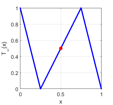
Figure 1. Graph of a map $T_{\omega}$, with $\gamma_{\omega}=2$.

A specific random driving could be $\sigma:S^{1}\to S^{1}$ given by $\sigma(\omega)=\omega+\alpha$ for some $\alpha\notin\mathbb{Q}$ and $\gamma_{\omega}=\gamma^{0}+\gamma^{1}\cdot\omega$ for $1<\gamma^{0}<\infty$ and $0<\gamma^{1}<\infty$, but only the ergodicity of $\sigma$ will be important for us. We consider the Banach spaces $\mathcal{B}_{\omega}$ to be the space BV of complex-valued functions of bounded variation.

To verify our general assumptions ((M1)), ((M2)), ((CCM)), ((A)), ((B)), ((C1)) - ((C7)) it suffices to check the assumptions (F1)–((F9)) This is done in a similar manner to the way in which the assumptions (E1)–(E9) of [4, Section 2.5] are checked in [4, Example 2.7.1] for transfer operators acting on the space of real-valued BV functions with different perturbations. Therefore we have only to verify assumptions ((C8)) and ((S)).

For each $\omega\in\Omega$ and each $n\in\mathbb{N}$ consider a sequence of shrinking balls $H_{\omega,n}$ containing the fixed point $x_{0}$ such that $x_{0}\in H_{\omega,n+1}\subseteq H_{\omega,n}$ for each $n\in\mathbb{N}$. Then assumption ((B)) is clearly satisfied. Furthermore the holes $H_{\omega,n}$ are chosen so that the assumption ((S)) is satisfied. Such holes $H_{\omega,n}$ are constructed in Section 2.7 of [4] as neighborhoods of extremal points of observation functions $h:M\to\mathbb{R}$.

Assumption ((S)) states that $\mu_{\omega,0}(H_{\omega,n})\leq\frac{|t|_{\infty}+W}{n}$. In this example, all fibre measures $\mu_{\omega,0}$ are Lebesgue and so the holes $H_{\omega,n}$ are neighbourhoods of $x_{0}$ of diameter no greater than $(|t|_{\infty}+W)/n$. Because the maps $T_{\omega}$ are locally expanding about $x_{0}$, for fixed $k>0$ one can find a large enough $n$ so that it is impossible to leave a small neighbourhood of $x_{0}$ and return after $k$ iterations. Therefore we can always find $n$ sufficiently large to guarantee that $\beta_{\omega,n}^{(k)}(\ell)=0$ for all $0<\ell<k$. If this were not the case, there must be a positive $\mu_{\sigma^{-(k+1)}\omega,0}$-measure set of points that (i) lie in $H_{\sigma^{-(k+1)}\omega,n}$, (ii) land outside $\ell<k$ of the holes $H_{\sigma^{-k}\omega,n},\ldots,H_{\sigma^{-1}\omega,n}$ for the next $k$ iterations, and then (iii) land in $H_{\omega,n}$ on the $k+1^{\mathrm{st}}$ iteration, which we have argued is impossible. On the other hand, the equality $\ell=k$ corresponds to the situation where points remain in the sequence of holes for all $k$ iterations, which will occur for a positive measure set of points. This immediately implies that $\beta_{\omega,n}^{(k)}(k)\neq 0$, and thus

$$\hat{q}_{\omega,n}^{(k)}(s) =(1-e^{is})e^{iks}\beta_{\omega,n}^{(k)}(k)=(1-e^{is})e^{iks}\frac{\mu_{\sigma^{-(k+1)}\omega,0}\left(\bigcap_{j=0}^{k+1}T_{\sigma^{-(k+1)}\omega}^{-j}(H_{\sigma^{-(k+1)+j}\omega,n})\right)}{\mu_{\omega,n}(H_{\omega,n})}.$$

Because the scaling $t_{\omega}$ varies along the orbit $\sigma^{-(k+1)}\omega,\ldots,\omega$, to simplify the above expression we assume that $1<\operatorname*{ess\sup}_{\omega}t_{\omega}/t_{\sigma^{-1}\omega}<\operatorname*{ess\inf}_{\omega}|T^{\prime}_{\omega}(x_{0})|$. This mild assumption on the variation of the scaling $t$ removes the “Case 2” considerations in Example 1 [4], and taking the limit as $n\to\infty$ gives

$$\hat{q}_{\omega,0}^{(k)}(s) =(1-e^{is})\frac{e^{iks}}{\left|DT_{\sigma^{-(k+1)}\omega}^{k+1}(x_{0})\right|}=(1-e^{is})\frac{e^{iks}}{\prod_{j=0}^{k}\gamma_{\sigma^{-(k+1)+j}}},$$

and thus we have

$$\theta_{\omega}(s)=1-(1-e^{is})\sum_{k=0}^{\infty}\frac{e^{iks}}{\left|DT_{\sigma^{-(k+1)}\omega}^{k+1}(x_{0})\right|}.$$

Applying Theorem 3.14 gives that

$$\varphi(s) =\exp\left(-(1-e^{is})\int_{\Omega}t_{\omega}\left(1-(1-e^{is})\sum_{k=0}^{\infty}\frac{e^{iks}}{\left|DT_{\sigma^{-(k+1)}\omega}^{k+1}(x_{0})\right|}\right)\,dm(\omega)\right)$$

$$=\exp\left(-(1-e^{is})\int_{\Omega}t_{\omega}\left(1-(1-e^{is})\sum_{k=0}^{\infty}\frac{e^{iks}}{\prod_{j=0}^{k}\gamma_{\sigma^{-(k+1)+j}\omega}}\right)\,dm(\omega)\right).$$

Note that since $1<\gamma\leq\gamma_{\omega}\leq\Gamma$, the series $\sum_{k=0}^{\infty}\frac{e^{iks}}{\prod_{j=0}^{k}\gamma_{\sigma^{-(k+1)+j}\omega}}$ converges absolutely to say $\Sigma_{\omega}(s)$ (which depends on $\omega$). Since $\Sigma_{\omega}(s)$ is not necessarily a geometric series, then $\varphi(s)$ is the characteristic function of a compound Poisson distribution which is not the Pólya-Aeppli distribution. It is unclear which specific compound Poisson distribution is represented by $\varphi(s)$.

Note that the tail of the series $\Sigma_{\omega}(s)$ is approximately given by $e^{-is}\sum_{k=N_{\omega}}^{\infty}(e^{is-\int_{\Omega}\log\gamma_{\omega}\,dm})^{k+1}$ where $N_{\omega}$ is the ($\omega$-dependent) time that it takes for the Birkhoff Ergodic Theorem to apply.

Example 5.2.

Pólya-Aeppli From Non-Random Slope and Random Holes: Taking the family of maps $\{T_{\omega}\}$ from the previous example, we now suppose that the slope of the central branch is constant; i.e. $DT_{\omega}(x_{0})=\gamma_{\omega}\equiv\gamma>1$ is constant. Then we have

$$\varphi(s) =\exp\left(-(1-e^{is})\int_{\Omega}t_{\omega}\left(1-(1-e^{is})\sum_{k=0}^{\infty}\frac{e^{iks}}{\gamma^{k+1}}\right)\,dm(\omega)\right)$$

$$=\exp\left(-\left(1-\gamma^{-1}\right)\left(\int_{\Omega}t_{\omega}\,dm(\omega)\right)\left(\frac{1-e^{is}}{1-e^{is}\gamma^{-1}}\right)\right).$$

Then $\varphi(s)$ is the characteristic function of a Pólya-Aeppli (geometric Poisson) distributed random variable $Z$ with parameters given by $\rho=\gamma^{-1}\in(0,1)$ and $\vartheta=(1-\gamma^{-1})\int_{\Omega}t_{\omega}dm$.

Example 5.3.

Pólya-Aeppli From I.I.D.  Maps and Holes: Now suppose that we are in the setting of the previous example where now we have two maps $T_{1}$ and $T_{2}$ chosen iid with probabilities $p_{1}$ and $p_{2}$ respectively. Again we let $x_{0}$ denote the common fixed point of the maps $T_{1}$ and $T_{2}$ and let $\gamma_{i}$ denote the slope of the map $T_{i}$ at $x_{0}$ for $i=1,2$. In this case $m$ is Bernoulli. Further suppose there are two values of $t$, namely $t_{1}$ and $t_{2}$, which are chosen iid with probabilities $\varrho_{1}$ and $\varrho_{2}$ respectively. Thus, using the fact that the $\gamma$ are chosen iid, we have that

(5.2) $$\int_{\Omega}\prod_{j=0}^{k}\gamma_{\sigma^{-(k+1)+j}\omega}^{-1}\,dm(\omega)=\left(\frac{p_{1}}{\gamma_{1}}+\frac{p_{2}}{\gamma_{2}}\right)^{k+1}=\left(\frac{p_{1}\gamma_{2}+p_{2}\gamma_{1}}{\gamma_{1}\gamma_{2}}\right)^{k+1}=:\zeta^{k+1}.$$

Note that $\zeta\in(0,1)$. Now since $t_{\omega}$ is independent of the $\gamma$ terms in the product appearing in (5.2) (since the product does not contain a $\gamma_{\omega}$), we can use (5.2) to write that

$$\int_{\Omega}t_{\omega}\left(1-(1-e^{is})\sum_{k=0}^{\infty}e^{iks}\prod_{j=0}^{k}\gamma_{\sigma^{-(k+1)+j}\omega}^{-1}\right)\,dm(\omega)$$

$$\qquad=\overline{t}\left(1-(1-e^{is})\sum_{k=0}^{\infty}e^{iks}\int_{\Omega}\prod_{j=0}^{k}\gamma_{\sigma^{-(k+1)+j}\omega}^{-1}\,dm(\omega)\right)$$

$$\qquad=\overline{t}\left(1-(1-e^{is})\sum_{k=0}^{\infty}e^{iks}\zeta^{k+1}\right)=\overline{t}\left(\frac{1-\zeta}{1-e^{is}\zeta}\right),$$

where $\overline{t}=\int_{\Omega}t_{\omega}\,dm=t_{1}\varrho_{1}+t_{2}\varrho_{2}$. Inserting this into the formula for $\varphi(s)$ gives

$$\varphi(s)=\exp\left(-\overline{t}(1-e^{is})\left(\frac{1-\zeta}{1-e^{is}\zeta}\right)\right)=\exp\left(-\overline{t}(1-\zeta)\left(\frac{1-e^{is}}{1-e^{is}\zeta}\right)\right),$$

which is the characteristic function of a Pólya-Aeppli ($\rho=\zeta\in(0,1)$ and $\vartheta=(1-\zeta)\overline{t}$) distributed random variable.

Example 5.4.

Standard Poisson from Random Maps and Random Holes:

Unlike the previous examples, we now provide an example in which the characteristic function produced from Theorem 3.14 is for a standard Poisson random variable rather than compound Poisson. We recall the setting of Example 4 of [4]. Let $\Omega=\{0,1,2,3\}^{\mathbb{Z}},$ with $\sigma$ the bilateral shift map, and $m$ an invariant ergodic measure.

To each letter $j=0,\dots,l-1$ we associate a rational number $v_{j}\in(0,1)\cap\mathbb{Q}$. We consider holes $H_{\omega,n}=B(v_{\omega_{0}},e^{-z_{n}(\omega)})$, where $\omega_{0}$ denotes the $0$-th coordinate of $\omega\in\Omega$ and the thresholds $z_{n}(\omega)$ are chosen such that assumption ((S)) holds. For each $\omega\in\Omega$ we associate a map $T_{\omega_{0}},$ where $T_{0},\dots,T_{3}$ are maps of the circle which we will take as $\beta$-maps of the form $T_{i}(x)=\beta_{i}x+r\pmod{1}$, with $\beta_{i}\in\mathbb{N}$, $\beta_{i}\geq 3$, and $0\leq r<1$ irrational and independent of $i$. Similar arguments to those given in [4, Example 4] show that our assumptions ((M1)), ((M2)), ((CCM)), ((A)), ((C1)) - ((C7)) are satisfied for this system. This is accomplished as in Example LABEL:ex_1, by showing that our assumptions (F1)–((F9)) follow from arguments similar to those of [4, Example 4] used to verify the assumptions (E1)–(E9). Furthermore, assumption ((B)) is satisfied by taking the Banach spaces $\mathcal{B}_{\omega}$ again to be BV.

Following the argument of [4, Example 4], it follows that a necessary condition to get $\beta_{\omega,n}^{(k)}(\ell)\neq 0$ for some $k\geq 0$ and $0\leq\ell\leq k$, and thus $\hat{q}_{\omega,0}^{(k)}(s)\neq 0$, is that the center $v_{(\sigma^{-(k+1)}\omega)_{0})}$ is sent to the center $v_{\omega_{0}}.$ Let $z$ be one of these rational centers. The iterate $T^{n}_{\omega}(z)$ has the form $T^{n}_{\omega}(z)=\beta_{\omega_{n-1}}\cdots\beta_{\omega_{0}}z+k_{n}r\,\pmod{1}$, where $k_{n}$ is an integer. Therefore such an iterate will never be a rational number, which shows that all $\hat{q}_{\omega,0}^{(k)}(s)=0$ for each $k\geq 0$, $\omega$, and each $s\in\mathbb{R}\backslash\{0\}$. Therefore we have $\theta_{\omega}(s)\equiv 1$, and so applying Theorem 3.14, we have

$$\varphi(s)=\exp\left(-(1-e^{is})\int_{\Omega}t_{\omega}\,dm(\omega)\right),$$

which is the characteristic function of a Poisson random variable with parameter $\vartheta=\int_{\Omega}t_{\omega}\,dm(\omega)$.

References

- [1] M. Abadi. Exponential approximation for hitting times in mixing processes. Math. Phys. Electron. J., 7:19 pp, 2001.
- [2] J. Atnip, G. Froyland, C. González-Tokman, and S. Vaienti. Thermodynamic formalism for random weighted covering systems. Communications in Mathematical Physics, July 2021.
- [3] J. Atnip, G. Froyland, C. González-Tokman, and S. Vaienti. Equilibrium states for non-transitive random open and closed dynamical systems. Ergodic Theory and Dynamical Systems, pages 1–23, Oct. 2022.
- [4] J. Atnip, G. Froyland, C. González-Tokman, and S. Vaienti. Thermodynamic formalism and perturbation formulae for quenched random open dynamical systems. arXiv preprint arXiv:2307.00774, 2022.
- [5] J. Atnip, N. Haydn, and S. Vaienti. Extreme value theory with spectral techniques: application to a simple attractor. 2023, submitted.
- [6] H. Aytac, J.-M. Freitas, and S. Vaienti. Laws of rare events for deterministic and random dynamical systems. Trans. Amer Math. Soc, 367:8229–8278, 2015.
- [7] D. Azevedo, A. C. M. Freitas, J. M. Freitas, and F. B. Rodrigues. Clustering of extreme events created by multiple correlated maxima. Physica D: Nonlinear Phenomena, 315:33–48, feb 2016.
- [8] A. Baker. Transcendental number theory. Cambridge University Press, London-New York,,, 1975.
- [9] T. Bogenschütz and V. M. Gundlach. Ruelle’s transfer operator for random subshifts of finite type. Ergod. Th. & Dynam. Sys, 15:413–447, 1995.
- [10] R. Brück and M. Büger. Generalized iteration. Computational Methods and Function Theory, 3(1-2, [On table of contents: 2004]):201–252, 2003.
- [11] J. F. C. Correia, A.C.M. Freitas. Cluster distributions for dynamically defined point processes. 2022. Preprint: CMUP[2022-35].
- [12] T. Caby, D. Faranda, S. Vaienti, and P. Yiou. Extreme value distributions of observation recurrences,. Nonlinearity, 34:118–163, 2021.
- [13] M. Carney, M. Holland, and M. Nicol. Extremes and extremal indices for level set observables on hyperbolic systems. Nonlinearity, 34(2):1136–1167, 2021.
- [14] M. Carney, M. Nicol, and H.-K. Zhang. Compound Poisson law for hitting times to periodic orbits in two-dimensional hyperbolic systems. J. Stat. Phys., 169(4):804–823, 2017.
- [15] M. Carvalho, A. C. M. Freitas, J. M. Freitas, M. Holland, and M. Nicol. Extremal dichotomy for uniformly hyperbolic systems. Dyn. Syst, 30(4):383–403, 2015.
- [16] J.-R. Chazottes, Z. Coelho, and P. Collet. Poisson processes for subsystems of finite type in symbolic dynamics. Stochastics and Dynamics, 9(03):393–422, 2009.
- [17] J.-R. Chazottes and P. Collet. Poisson approximation for the number of visits to balls in non-uniformly hyperbolic dynamical systems. Ergodic Theory and Dynamical Systems, 33(1):49–80, 2013.
- [18] L. H. Y. Chen and A. Barbour. Stein’s method and applications, volume 5. World scientific, 2005.
- [19] H. Crauel. Random probability measures on Polish spaces, volume 11 of Stochastics Monographs. Taylor & Francis, London, 2002.
- [20] H. Crimmins. Stability of hyperbolic Oseledets splittings for quasi-compact operator cocycles. arXiv:1912.03008 [math], Dec. 2019. arXiv: 1912.03008.
- [21] H. Crimmins and B. Saussol. Quenched Poisson processes for random subshifts of finite type. 2020, https://arxiv.org/pdf/2011.13610.pdf.
- [22] D. Dragičević, G. Froyland, C. González-Tokman, and S. Vaienti. Almost sure invariance principle for random piecewise expanding maps. Nonlinearity, 31(5):2252–2280, May 2018.
- [23] W. Feller. An introduction to probability theory and its applications. Vol. I. John Wiley & Sons, Inc., New York-London-Sydney, third edition, 1968.
- [24] A. C. M. Freitas, J. M. Freitas, M. Magalhaes, and S. Vaienti. Point processes of non stationary sequences generated by sequential and random dynamical systems. Journal of Statistical Physics, 181:1365–1409, 2020.
- [25] A.-C. M. Freitas, J.-M. Freitas, and M. Magalhes. Convergence of marked point processes of excesses for dynamical systems. J. Eur. Math. Soc. (JEMS), 20:2131–2179, 2018.
- [26] A.-C. M. Freitas, J.-M. Freitas, M. Magalhes, and S. Vaienti. Point processes of non stationary sequences generated by sequential and random dynamical systems. Journal of Statistical Physics, 181:1365–1409, 2020.
- [27] A. C. M. Freitas, J. M. Freitas, and M. Todd. The compound Poisson limit ruling periodic extreme behaviour of non-uniformly hyperbolic dynamics. Communications in Mathematical Physics, 321(2):483–527, 2013.
- [28] A. C. M. Freitas, J. M. Freitas, and S. Vaienti. Extreme value laws for non stationary processes generated by sequential and random dynamical systems. Annales de l’Institut Henri Poincaré, 53(3):1341–1370, 2017.
- [29] J. M. Freitas, N. Haydn, and M. Nicol. Convergence of rare event point processes to the Poisson process for planar billiards. Nonlinearity, 27(7):1669, 2014.
- [30] G. Froyland, S. Lloyd, and A. Quas. A semi-invertible Oseledets theorem with applications to transfer operator cocycles. Discrete and Continuous Dynamical Systems, 33(9):3835–3860, Mar. 2013.
- [31] S. Gallo, N. Haydn, and S. Vaienti. Number of visits in arbitrary sets for -mixing dynamics. Annales de l’Institut Henri Poincaré - Probabilités et Statistiques, 2022, to appear.
- [32] N. Haydn and Y. Psiloyenis. Return times distribution for markov towers with decay of correlations. Nonlinearity, 27(6):1323, 2014.
- [33] N. Haydn and S. Vaienti. The distribution of return times near periodic orbits. Probability Theory and Related Fields, 144:517–542, 2009.
- [34] N. Haydn and S. Vaienti. Limiting entry times distribution for arbitrary null sets. Communication in Mathematical Physics, 378:149–184, 2020.
- [35] N. Haydn and K. Wasilewska. Limiting distribution and error terms for the number of visits to balls in non-uniformly hyperbolic dynamical systems. Discr. Cont. Dynam. Syst., 36(5):2585–2611, 2016.
- [36] N. Haydn and F. Yang. A derivation of the Poisson law for returns of smooth maps with certain geometrical properties. Contemporary Mathematics Proceedings in memoriam Chernov, 2017.
- [37] M. Hirata. Poisson law for axiom a diffeomorphisms. Ergodic Theory and Dynamical Systems, 13(3):533–556, 1993.
- [38] M. Hirata, B. Saussol, and S. Vaienti. Statistics of return times: A general framework and new applications. Communication in Mathematical Physics, 206:33–55, 1999.
- [39] J. Hüsler. Extreme values of nonstationary random sequences. J. Appl. Probab., 23(4):937–950, 1986.
- [40] N. Johnson, A. Kemp, and S. Kotz. Univariate discrete distributions. 2005, 3rd ed.
- [41] G. Keller. Rare events, exponential hitting times and extremal indices via spectral perturbation†. Dynamical Systems, 27(1):11–27, 2012.
- [42] G. Keller and C. Liverani. Stability of the spectrum for transfer operators. Annali della Scuola Normale Superiore di Pisa-Classe di Scienze, 28(1):141–152, 1999.
- [43] G. Keller and C. Liverani. Rare events, escape rates and quasistationarity: Some exact formulae. Journal of Statistical Physics, 135(3):519–534, 2009.
- [44] Y. Kifer and A. Rapaport. Poisson and compound Poisson approximations in conventional and nonconventional setups. Probability Theory and Related Fields, 160(3-4):797–831, 2014.
- [45] Y. Kifer and F. Yang. Geometric law for numbers of returns until a hazard under -mixing. arXiv preprint arXiv:1812.09927, 2018.
- [46] E. Lukacs. Characteristic functions. Griffin, London, 2nd ed. rev. and enl edition, 1970. OCLC: 489835032.
- [47] V. Mayer and M. Urbański. Countable alphabet random subhifts of finite type with weakly positive transfer operator. Journal of Statistical Physics, 160(5):1405–1431, 2015.
- [48] V. Mayer, M. Urbański, and B. Skorulski. Distance Expanding Random Mappings, Thermodynamical Formalism, Gibbs Measures and Fractal Geometry, volume 2036 of Lecture Notes in Mathematics. Springer Berlin Heidelberg, Berlin, Heidelberg, 2011.
- [49] V. Mayer and M. Urbański. Random dynamics of transcendental functions. Journal d’Analyse Mathématique, 134(1):201–235, Feb. 2018.
- [50] F. Pène and B. Saussol. Back to balls in billiards. Communications in mathematical physics, 293(3):837–866, 2010.
- [51] F. Pène and B. Saussol. Poisson law for some non-uniformly hyperbolic dynamical systems with polynomial rate of mixing. Ergodic Theory and Dynamical Systems, 36(8):2602–2626, 2016.
- [52] F. Pène and B. Saussol. Spatio-temporal Poisson processes for visits to small sets. Israel Journal of Mathematics, 240(2):625–665, 2020.
- [53] B. Pitskel. Poisson limit law for markov chains. Ergodic Theory Dynam. Systems, 11(3):501–513, 1991.
- [54] J. Rousseau, B. Saussol, and P. Varandas. Exponential law for random subshifts of finite type. Stochastic Process. Appl., 124(10):3260–3276, 2014.
- [55] F. Yang. Rare event process and entry times distribution for arbitrary null sets on compact manifolds. In Annales de l’Institut Henri Poincaré, Probabilités et Statistiques, volume 57, pages 1103–1135. Institut Henri Poincaré, 2021.
- [56] H. Zhang and B. Li. Characterizations of discrete compound Poisson distributions. Communications in Statistics - Theory and Methods, 45(22):6789–6802, 2016.
- [57] X. Zhang. A Poisson limit theorem for Gibbs-Markov maps. Dynamical Systems, pages 1–16, Nov. 2020.
- [58] R. Zweimüller. The general asymptotic return-time process. Israel J. Math., 212:1–36, 2016.
- [59] R. Zweimüller. Hitting times and positions in rare events. Annales Henri Lebesgue, 5:1361–1415, 2022.