One-Time Compilation of Device-Level Instructions for Quantum Subroutines

Abstract

A large class of problems in the current era of quantum devices involve interfacing between the quantum and classical system. These include calibration procedures, characterization routines, and variational algorithms. The control in these routines iteratively switches between the classical and the quantum computer. This results in the repeated compilation of the program that runs on the quantum system, scaling directly with the number of circuits and iterations. The repeated compilation results in a significant overhead throughout the routine. In practice, the total runtime of the program (classical compilation plus quantum execution) has an additional cost proportional to the circuit count. At practical scales, this can dominate the round-trip CPU-QPU time, between 5% and 80%, depending on the proportion of quantum execution time.

To avoid repeated device-level compilation, we identify that machine code can be parametrized corresponding to pulse/gate parameters which can be dynamically adjusted during execution. Therefore, we develop a device-level partial-compilation (DLPC) technique that reduces compilation overhead to nearly constant, by using cheap remote procedure calls (RPC) from the QPU control software to the CPU. We then demonstrate the performance speedup of this on optimal pulse calibration, system characterization using randomized benchmarking (RB), and variational algorithms. We execute this modified pipeline on real trapped-ion quantum computers and observe significant reductions in compilation time, as much as 2.7x speedup for small-scale VQE problems.

I Introduction

Current quantum computers are far from the requisite physical error rates and the qubits needed to support quantum error correction. While hardware developers race toward this long-term goal, there is wide interest in finding near-term use cases for quantum computers. One such class of problems is what we call qci problems, essentially programs, algorithms, or routines which repeatedly communicate with a quantum computer and make decisions about subsequent actions based on the outcomes. This class encompasses routines at both the algorithm/application layer as well as further down the hardware-software stack.

QCI problems include promising variational quantum algorithms (VQA) like vqe [29] and quantum alternating operator ansatz (QAOA) [17], which aim to solve classically hard quantum chemistry and optimization problems respectively. In this model, the high-level algorithm requires repeated execution of programs whose contents depend on the results from the previous programs. These algorithms often use the same underlying circuit structure, but vary parameters, like rotation angles.

Beyond high-level applications, there are many characterization and calibration routines that fall into this category. Quantum computers currently require extensive amounts of characterization which consists of a set of processes that probe the quantum computer for its noise sources. Because the noise in a system can be time-dependent, these routines involve long sequences of operations. Every iteration can correspond to new sequence lengths or different measurement bases. Common characterization routines, such as rb [23] and gst [1] can’t be strictly viewed as instances of the qci framework as their iterations do not necessarily depend on previous measurements. They do involve sequential execution of circuits, and the user may choose to alter the routine, like running more circuits of a particular type for higher precision.

Because many quantum systems are susceptible to noise resulting in parameter drifts, they need to be routinely calibrated. Program operations on a quantum system correspond to hardware-specific pulses applied to subsets of qubits. The amplitude, phase, frequency, and duration of these pulses must be calibrated in order to execute the desired operations with a high success rate. In naive versions, this pipeline can be very simple, a sequence of short circuits of individual pulses which scan over each of these parameters to find optimal points. Alternative approaches which can reduce the shot count (the number of times the qubits are measured) overheads are adaptive. Here, again, short circuits are executed but instead of being a scan, we can update a Bayesian inference model [39] to decide which pulse to try next.

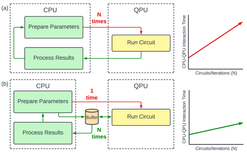
Figure 1: The pipeline for execution of quantum programs on hardware involves a sequence of compilation steps - circuit level, pulse level, and device level. Device level compilation involves the translation of circuit elements to control hardware primitives. For current applications and routines (a) the kernel is compiled every iteration and for every new set of circuits. Device compilation overheads scale as a function of the number of circuits. (b) Many circuits change in only small ways and have predictable effects on the underlying driver instructions. We propose partial compilation of the kernel which happens exactly once. In every iteration, we pass small amounts of information between the CPU and QPU and modify pulse execution appropriately.

Common amongst each of these examples is a repeated back and forth between the quantum computer and the classical computer with varying amounts of intermediate classical decision-making. Classical overheads are often ignored - we are willing to sacrifice large upfront classical compute times to optimize and compile input programs with the promise that quantum computers will provide sufficient speedup to accommodate this overhead. Most quantum computing architectural studies have focused on optimization relatively high in the hardware-software stack, prioritizing circuit-level and pulse-level improvements. What has largely been ignored is the practical costs of preparing and executing these optimized programs on hardware. This is typically assumed to be very low relative to the execution time of the quantum program.

Device-level compilation refers to the conversion of the high-level intermediate representation of quantum gates or pulses to machine code runnable on the control hardware, similar to the translation from classical instruction set architecture (ISA) to executable binaries. In the current quantum computing stack, device-level compilation corresponds to the construction of a kernel that is run on the qpu - the electronics that control the quantum hardware.

For single-circuit applications, this amounts to only a single round of kernel compilation. For qci problems, which require large numbers of circuits and/or iterations, repeated kernel compilation becomes substantial. This is illustrated in Fig. 1(a). Repeated sequential compilation of circuits, either by adding new subcircuit elements and/or modifying circuit parameters such as the angle of rotation, is expensive when the final solution for these algorithms requires hundreds or thousands of passes through the classical-quantum loop. Prior work has focused on reducing the compilation costs upstream from the actual execution of the circuit on hardware, for example, circuit optimization, gate decompositions, and scheduling. While minimizing this upfront compilation time is important, it often occurs only once during the execution of the entire program. Downstream optimizations, like pulse generation, might be repeated. The work in [9] proposes partial compilation techniques for variational algorithms to reduce the computational overhead of these repeated optimizations by only recompiling small sections of the circuit.

We propose a partial compilation technique, further downstream, at the interface of hardware instructions, which currently are always repeated for each new circuit. In this work, we modify this pipeline to compile only once to device-level instructions and instead perform inexpensive calls outside the qpu kernel to update instruction lists or circuit parameters which can be quickly incorporated into the existing executables, essentially extending partial-compilation all the way into the kernel. This technique is outlined in Fig. 1(b). By spinning up the qpu exactly once per program we further reduce computational overhead for qci problems. This, of course, assumes that the isa of the control processor allows for partially compiled binaries. However, the novelty of our proposal lies in creating a pipeline that utilizes this isa to reduce compilation costs in qci problems which involve repeated context switches between the classical and quantum computer.

The utility of this one-time dlpc method depends on the need for hardware re-calibration and circuit re-optimization. For problems like traditional VQE, changes in parameters do not substantially affect the circuit optimizations. For problems where the structure does change iteratively, forced re-optimization every cycle has marginal benefits at the cost of another compilation loop and instead, this exit should be forced only periodically once changes have accumulated. Current hardware parameters do drift, requiring periodic re-calibration of the entire machine. This then necessitates circuit re-optimization (e.g. remapping) and kernel re-compilation since the hardware parameters have changed. In both these cases, we must recompile the kernel, limiting the effectiveness of the dlpc technique. However, these events happen relatively infrequently, thereby still saving on compilation costs on most iterations. Also, given dlpc’s application to calibration, and recent development in calibration routines that are dynamic and interleaved between computation (like in [27]), our proposed technique shows an advantage over the naive approach even when the system needs to be re-calibrated and re-optimized

The major contributions of this work are as follows:

1. We identify that quantum operations (gates or pulses) have invariant underlying structures at the machine level. This enables parameterization of corresponding machine code which can dynamically adjust to changing circuit or pulse level parameters.

2. We extend the idea of partial compilation to the device level, enabling one-time compilation of machine code run on the qpu, reducing to nearly iteration-independent compilation scaling.

3. DLPC reduces net runtime overhead for the class of qci problems, or any iterative program, by demonstrating a potential speedup of up to 2.7x, 7.7x, and 2.6x for representative vqe, optimal calibration, and rb programs, respectively. For interleaved recalibration routines, we observe an even greater advantage of DLPC - we only compile the kernel for the circuits once but we compile the kernel only once for the system probes and the calibration routines.

4. We expand DLPC to the general case of fixed gate-set hardware to accommodate cloud-based quantum platforms.

5. We demonstrate this routine on a trapped-ion quantum computer by running simple vqe programs and measuring the compilation and execution time speedup.

II Background

II-A Compilation for QCI problems

The hybrid nature of qci programs make compilation for them an interesting problem. Every context switch between the cpu and qpu incurs a runtime overhead of re-compiling the quantum program with a new set of parameters over each iteration. As the number of iterations increase, this compilation overhead can balloon out of proportion. However, the term compilation is used in the field as a blanket term for a multi-step process in the software pipeline. In the rest of this section, we break this compilation process into a few fundamental components, and highlight the one our proposal optimizes.

In a hardware-accelerator model of execution [40, 37, 28, 4], a quantum program can be divided into classical components that run on the cpu, and quantum components that run on the qpu. The classical components are compiled by the high-level general-purpose language that they are represented in. The quantum components are compiled by the compiler built for the high-level domain-specific language used to represent a quantum circuit. We primarily focus on the latter, with quantum components being gate-level operations. Compiling quantum components in the nisq [30] era typically adheres to the following pipeline. The high-level gate instructions go through a hardware-agnostic optimizations, followed by a compiler pass to transform the operations to a gate set specific to the target quantum hardware platform. Operations are then appropriately scheduled and mapped in relation to the hardware architecture. This is followed by a conversion to pulses, which may be further optimized to reduce pulse length and account for known sources of error in the physical system. These pulses are then compiled to appropriate device-level instructions (essentially an assembly representation) which depend on the control electronics being used in the experimental setup. Finally, device-level instructions are translated into binaries which will be executed on the control electronics.

In this work, we are focused on this final step - device-level compilation,and reducing redundant repetitions of this stage during qci applications.

II-B Control System

For the device-level compilation pipeline, we use an artiq based control system [35] to write and execute qci programs. It is a modular control software framework that builds upon artiq [2, 19]. artiq is a real-time control software solution that uses a hardware accelerator model of execution for quantum computing programs. The program can be offloaded to specialized hardware components allowing for greater efficiency as compared to running the program on a general purpose cpu alone. In the case of artiq, this specialized hardware component is an fpga board optimized for real-time precision.

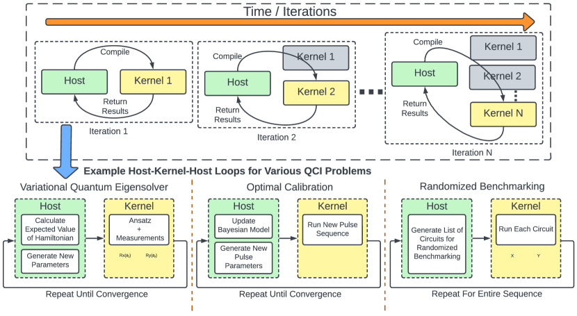
Figure 2: Typical compilation pipelines for qci programs follow the control flow shown here. Each iteration of the program results in the compilation of a new kernel. Examples of host-kernel-host execution loops are shown. Over each iteration - in a vqe program, the host generates parameters based on the expected value of the Hamiltonian; in an optimal calibration routine, the host generates new pulse parameters to converge to an optimal pulse sequence; in an rb routine, the kernel executes a new circuit from a pre-generated list of benchmarking circuits.

An artiq program typically consists of 2 parts - host and kernel. The host refers to the part of the program executed on a classical machine, which we refer to as the cpu. The kernel is performed on the real-time control fpga board responsible for managing instructions on the quantum computer, which we refer to as the qpu. For example, a classical optimizer is part of the host block while the real-time execution is defined in the kernel block of the program. The kernel is compiled to binary files to be run on the qpu using artiq’s compiler. The program on the cpu communicates with the qpu over an Ethernet connection.

Communication with the host from within the kernel can be done through rpc. These rpc can be synchronous, in which case the kernel waits for the call to return, or asynchronous where the call is executed on the host while the kernel continues with its execution. For example, storing the measurement results of a circuit is an asynchronous rpc.

III Motivation

Quantum computers require significant amounts of setup before they are operational for computation. For every type of underlying hardware the device must be extensively characterized and its operations calibrated. Such routines, similar to variational algorithms, require constant interaction between the quantum and classical processing, i.e. there is no single shot pass which prepares the hardware into a runnable state. Multiple rounds of circuit preparation, execution, and subsequent classical post-processing are performed, which can incur significant compilation overhead. In this section, we further motivate the need for our partial-compilation technique for classes of calibration, characterization, and applications which depend on qci routines. A sample schematic for these routines can be seen in Fig. 2.

III-A Optimized Calibration

Quantum computers require high fidelity (low error) state preparation, operations, and measurements. The parameters of a quantum system drift with time resulting in systematic errors that affect the fidelities. This motivates the need for periodic calibration of the system to appropriately adjust gate pulse parameters. A naive scan across parameters to re-calibrate the system can be expensive, and there have been recent proposals to make these calibration routines optimal [25, 16, 26, 39]. These calibration routines involve quantum-classical interfacing, requiring analysis and computation on the classical computer every iteration as it attempts to converge to the optimal pulse parameters. This adds an overhead associated with recompiling the pulse sequence every iteration. In general, calibration procedures do not calibrate operations on all N qubits of the system simultaneously, and instead characterize subsets, e.g. every pair of connected qubits, which requires an additional factor of $O(N^{2})$ machine compilations. In this work, we explore Stace, et al.’s proposal on using Bayesian inference for optimizing pulse sequences [39] as an example to demonstrate the compilation overhead. Their work shows the calibration of single and two-qubit gate pulse sequences using a Bayesian inference model on the classical computer, realized using piece-wise constant amplitude-modulated pulse sequences. Because these calibration routines operate at the level of pulses, the only relevant layers from the compilation pipeline here are pulse-level and device-level compilation. The pulse-level compilation here adds no overhead as there is no optimization being performed, instead these routines are used to find the optimal pulse for the given system. Device-level compilation, however, is required to compile the pulses down to executable binaries which by default is done each cycle.

III-B System Characterization

System characterization refers to routines that are run on a quantum computer to assess the noise in the system and are often used in conjunction with calibration. Widely used characterization routines include gst [1], rb [23, 24], cycle benchmarking [8], and empirical direct characterization [7]. Most of these routines involve sequential execution of series of generated circuits, with a significant overhead associated with compiling large numbers of circuits each to be run only a few times on the quantum computer. We focus on rb as an illustrative example of the present device-compilation overhead. rb runs circuits with increasingly longer sequences of randomly generated gates [23]. Similar to calibration, system operators characterize subsets, e.g. every pair of connected qubits, resulting in an additional factor of $O(N^{2})$ machine compilations [18].

III-C Variational Quantum Eigensolver

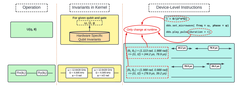
Figure 3: Kernel execution of parameterized quantum operations. Consider a gate $U$ acting on qubit $q$ with a parameter $\theta$. First, the hardware-specific qubit invariants are retrieved from the persistent dataset. Here, invariant parameters are the qubit frequency $\omega$, Rabi frequency $\Omega$, and phase associated with the gates $\phi$. The desired pulse is configured by setting $\omega$ with a offset $\phi$ on the direct digital synthesizer (DDS), and $\Omega$ and the gate parameter $\theta$ are used to calculate the pulse duration, here from [21]. The DDS plays the appropriate pulse sequence for the dynamically and analytically calculated duration. The kernel can be compiled just once with the invariant parameters, while the variables are supplied during runtime at each iteration.

For near-term quantum devices, a promising application is vqe. vqe is a hybrid, iterative algorithm that uses the variational method [13] and can be used to find the ground state energy of a molecule [29]. A Hamiltonian (essentially a large paramterized matrix) is a quantum mechanical operator which corresponds to the total energy of a system. A parameterized quantum circuit, or ansatz, with measurements corresponding to the constructed Hamiltonian is then iteratively executed with varying parameters until the expected value of the Hamiltonian converges to the optimal value. On each iteration, the next set of parameters and set of measurements for the circuit are determined by a classical optimizer which runs on the cpu, as opposed to the ansatz circuit, which is executed on the qpu.

At the gate-level, a vqe program remains invariant with respect to the type of gates being used across iterations. However, the changing parameters of these gates over each iteration have cascading effects on the resultant pulses and device-level code. In the naive pipeline, this results in these components being re-compiled every iteration. Past work, like [9], propose compiler optimizations and partial compilation techniques to reduce the pulse-level re-compilation overhead. In Section VI we show that for real small-scale systems the device-level compilation time can be significant, and demonstrate how our proposed routine reduces this overhead to being nearly constant.

IV Control Flow for QCI Routines

Currently, the control software design for a qci program begins in the host. In an optimal calibration routine, this is where the initial pulse parameters are declared, while in a vqe program the initial guess for the ansatz parameters are declared here. This is followed by an invocation of a kernel function that runs the pulse sequence or the ansatz circuit respectively on the quantum system with the given parameters. The control is then transferred back to the host. Based on measurement results the classical optimizer generates a new set of parameters for the next iteration.

In the existing control flow, each iteration of the qci routine calls a kernel function, as seen in Fig. 2. Each call involves device-level compilation passes which have an associated runtime cost associated with them. This cost consists of kernel compilation, kernel uploading, and kernel scheduling. Kernel compilation involves the time it takes to optimize and compile the kernel code to be executed on the control hardware. This depends on the complexity of the kernel. Kernel uploading is the time it takes to upload the compiled kernel onto the control hardware. This is determined by the size of the compiled kernel and the communication time between the host and control hardware. Finally, kernel scheduling consists of the time it takes to schedule the compiled kernel on the control hardware execution queue. This is affected by whether there are any other processes that need to be terminated before the current one is allowed to execute.

All of these components repeated in each iteration affect the runtime performance of a qci program. We identify an inherent underlying shared structure in the kernel code of qci programs, as in Fig. 3. For example - vqe programs always execute the same circuits, only varying the gate parameters at each iteration; an optimal calibration routine fixes a general structure for the pulse sequence while varying a subset of the pulse parameters, like the frequency and the number of segments in a piece-wise segmented sequence remain fixed in [39], while the amplitude and total pulse duration change every iteration; a rb routine runs a sequence of circuits for varying number of gates per circuit but all of these gates are randomly sampled from a set pool of operators which can be precompiled. This underlying structure results in large parts of the kernel being invariant at runtime. This invariance lends the device-level code to be partially compiled, with dynamic parameters passed in at runtime. The following section describes our dlpc technique that saves on the repeated kernel compilation, uploading, and scheduling time over each iteration of the program.

V DLPC

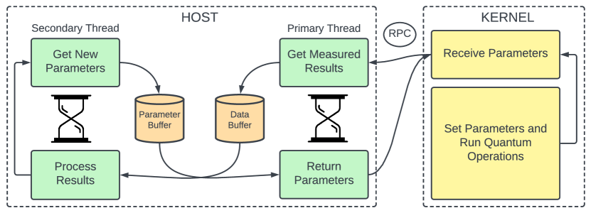
Figure 4: Our proposed partial-compilation routine for qci programs. The kernel is compiled only once, and at runtime receives new parameters through rpc at each iteration. The host program uses a multi-threaded produces-consumer pattern to wait on the latest measurement results and appropriately generates new parameters or sends a sentinel value conveying convergence.

In principle, the simplest way to optimize device-level compilation is to avoid re-compiling blocks of kernel code every iteration. We propose a routine that has a kernel block compiled only once and gets new parameters from the classical computer at each iteration.

There are some constraints that need to be considered while designing this routine. Consider the example of a vqe program - once the program enters the kernel to execute the first iteration of the ansatz, the control flow has to stay in the kernel until the last iteration of the ansatz is run. Failure to do so results in re-compilation of the kernel. The classical optimizer has to run on the host, as the hardware on the qpu lacks the ability to perform computationally intensive tasks. This requires the control flow in the kernel to wait for updated ansatz parameters between iterations.

Given these constraints, we propose the following device-level partial compilation (dlpc) routine. On the cpu, we divide the execution of the program into two threads - the main thread that runs the primary control flow of the host, and a secondary thread that runs the optimizer function. These threads wait on 2 buffers respectively - a parameter buffer and a results buffer. The parameter buffer stores the new parameters for the next iteration of the qci program, and the results buffer stores the latest measurement results from the operations executed on the quantum system. In this routine, these two threads will work similar to a multi-threaded producer-consumer pattern. The qpu consists of just one thread for kernel execution. The qci routine starts with the secondary thread waiting on the data buffer and the main thread calling the kernel function for the first time with initial parameters. This is the only time the kernel is compiled and uploaded on the qpu.

In the case of the VQE example, the kernel function is terminated only when the optimal expectation value is reached. In the first iteration, the kernel executes the quantum operations with the initial parameters and then makes a synchronous rpc to retrieve the next set of parameters. Because this is a synchronous rpc, it waits for the call to return before resuming execution. This rpc invokes a function on the main thread which first adds the latest measurement results into the data buffer and then waits on the parameter buffer. This resumes execution on the secondary thread running the optimizer’s objective function. This secondary thread performs the intensive classical computation and analyses based on the measurement results, generates a new set of parameters, adds them to the parameter buffer, and then goes back to waiting on the data buffer. This resumes execution on the main thread that was waiting on the parameter buffer. The function on the main thread returns these new parameters back to the kernel, which resumes its execution by running the quantum operations again with the new parameters, appropriately adjusting pulse amplitudes, frequencies, etc. The routine continues until the optimizer converges, at which point it adds a sentinel value to the parameter buffer. This results in the main thread returning a Boolean flag back to the kernel that terminates its execution. This routine is illustrated in Fig. 4. This partial-compilation routine can be adapted to any qci routine, like characterization or optimal calibration, as they follow the general structure of interleaving execution on the qpu with some amount of computation on the cpu to inform the next iteration of the routine.

Here the kernel is compiled to the qpu only once but is not yet executable as the parameters for the quantum operations are variable. Over each iteration of the qci program, this partially compiled block gets the latest parameters which are appropriately added to the compiled binaries and then executed on the qpu. The only overhead for each iteration of the program is the communication round-trip time taken by the synchronous rpc. However, this communication round-trip time is also incurred by the existing device-compilation pipeline over every iteration but is generally negligible, in addition to the time taken to compile, upload and schedule the kernel block each time. The multi-threaded producer-consumer design pattern using two shared data structures allows users to continue using off-the-shelf optimizer functions while avoiding race conditions.

The kernel block for other routines, like characterization, can be written to only include functions that correspond to operators in the pool. The kernel can be parameterized to receive a simple representation of the circuit, and at runtime the circuit can be executed by appropriately calling the function that corresponds to the gates in the circuit representation. As each circuit is composed of the same set of gates, this results in the kernel being compiled only once. Depending on the memory available on the qpu, a block of circuit representations that parameterize the kernel can be uploaded through a rpc, much like the parameters for qci routines. This partial-compilation technique saves on the overhead added by compiling each circuit of the sequence by leveraging their structure. Given that the number of circuits executed as part of these benchmarking routines can be very large, our one-time partial compilation technique offers a significant performance benefit. This strategy could also be used for hardware with long periods of uptime, e.g. commercial hardware accessed via the cloud which should just listen for new user gate sequences. This is explored in Sec VII-B.

The novelty of the proposed dlpc routine lies in identifying the shared structure between iterative runs of qci problems and building a device-level partial compilation pipeline that uses an always-on kernel and producer-consumer multi-threaded design pattern on the host. This pipeline utilizes the shared structure in these problems with a control processor whose isa supports partially-compiled executable binaries.

VI Results

To demonstrate the dlpc technique on an experimental system we use a trapped-ion quantum system described in [21]. It is controlled by a artiq based control software solution [35] and uses a Kasli 2.0 board [19] as the qpu. At the time of this demonstration, the system was only capable of running operations on a single-qubit. As a result, the experimental demonstration of the pipeline is limited to single-qubit vqe problems, but the dlpc routine can be used on any number of qubits and operations. We use experimental results to demonstrate our proposal’s immediate viability.

In order to show the performance of the partial-compilation technique on qci problems involving multiple qubits, we use a functional simulator [36] that gives us accurate compile times for the kernel. The runtime of these routines is then estimated using true operation times on the trapped-ion quantum computer described above in addition to the compile time from the simulator. These operation times are $5\mu s$ for single-qubit operations and $150\mu s$ for two-qubit operations.

VI-A Experimental Results

For the experimental demonstration of the dlpc routine, we execute 2 single-qubit toy vqe programs. For consistency, both the ansatz circuits are sampled over 300 shots for each iteration of the vqe program. In the single-parameter circuit, this results in 300 runs of the circuit followed by a $\sigma_{z}$ measurement, while in the two-parameter circuit, it involves 100 runs each of the circuits followed $\sigma_{x},\sigma_{y},$ and $\sigma_{z}$ measurements respectively. In both cases, the data has been collected over 10 runs of the vqe program. The results from this demonstration are presented in Fig. 5.

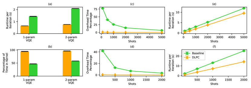
Figure 5: Demonstration of dlpc technique on a trapped-ion quantum computer. (a) Runtime comparison between the baseline and dlpc approaches. On average, the baseline approach takes 2.2x more time relative to the DLPC technique for the 1-param vqe demonstration, and 2.7x more time for the 2-param vqe demonstration. (b) Percentage of time spent executing the circuit on the quantum computer. On average, the dlpc technique results in 94.4% of time spent in the kernel, relative to 46.8% using the baseline approach for the 1-param vqe. For the 2-param vqe, on average 96.1% of time is spent in the kernel when using dlpc relative to 57.9% for the baseline approach. (c)-(d) Compilation overhead as a percentage of total runtime for increasing number of shots for the 1-param and 2-param vqe experiments respectively. (e)-(f) The runtime per iteration as a function of the number of shots for the 1-param and 2-param vqe experiments respectively.

When sampling over 300 shots, the naive compilation approach takes, on average, $\sim$2.2x more time for the 1-parameter vqe and $\sim$2.7x for the 2-parameter vqe. The latter shows a larger speedup as it involves a bigger kernel as kernel compilation is related to the number of gates. In Fig 5(b) we show the percentage of time each algorithm spends in the kernel executing the circuit. For the naive case, this percentage is $\sim$46.8% for the 1-parameter vqe experiment and $\sim$57.9% for the 2-parameter vqe experiment, while when using our technique it is $\sim$94.4% and $\sim$96.1% respectively. When using the naive approach, a large portion of the execution time is spent in re-compiling the kernel at the device level. However, in applications like vqe, as the size of the problem and the required number of shots increase, the execution time is dominated by the circuit time [10]. This results in a diminishing advantage of our compilation technique, which has been demonstrated in the Fig 5(c)-(d). In the worst case, there is always some constant advantage with our technique, but the extent of this advantage depends on the vqe techniques [14] used and the ongoing research in improving gate times [38] and reducing vqe shot budgets [15]. Our proposal’s real strength is applications that require many different circuits but which get run relatively few times.

VI-B Simulation Results

We demonstrate the performance of our dlpc technique for optimal calibration routines and system characterization schemes by running these routines in simulation to get true compile times and estimated runtimes of the experiments.

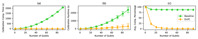
Figure 6: Demonstration of the dlpc technique relative to the baseline approach for the optimal calibration routine proposed in [39]. (a) dlpc compiles the kernel only once, resulting in a constant compilation cost of 1.2 seconds on average. The baseline approach compiles the kernel for every single iteration of the routine which scales quadratically. (b) The runtime for dlpc and baseline approaches grows quadratically as the system size increases, however, the baseline approach grows much faster due to the dominant compilation overhead. (c) The compilation time as a percentage of the total runtime. For the dlpc approach, this percentage diminishes as the system size grows, while in the baseline approach, this is over 80%.

Fig. 6 presents the performance advantage of the dlpc technique for the optimal calibration procedure proposed in  [39]. Their proposal has a calibration routine for single-qubit pulses using 2 parameters and for two-qubit routines using 5 parameters. For $N$ qubits, the total number of parameters can then be represented as $2N+5\binom{N}{2}$. The number of iterations required for convergence is proportional to the number of parameters in the system, resulting in a superlinear scaling of iterations with qubit size. The parameterized kernel for this routine takes in the qubits being optimized, the amplitude modulations, and the pulse duration as parameters for the piece-wise constant pulse. Our technique compiles this kernel to the device only once, while in the naive approach, this compilation cost has at least quadratic scaling. Their calibration routine claims to converge to the optimal routines using 50-100 shots per experiment. Given single and two-qubit pulses on the order of the single and two-qubit gate times mentioned above, the total runtime of the experiment is then dominated by the compilation time. This results in the total runtime scaling similar to the compilation time of the routine.

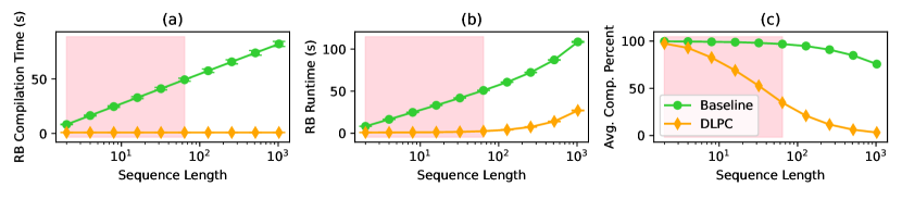
Figure 7: dlpc relative to the baseline approach for rb. The shaded region indicates the typical sequence lengths for current machines which do not exceed $\sim 10^{2}$ (a) The dlpc routine results in an average constant compilation cost of 0.87 sec. For the baseline approach, compilation cost scales with a growing sequence length. (b) The runtime for dlpc and baseline approaches grows as the number of rb sequences increase, however, the baseline approach grows much faster due to the dominant compilation overhead. (c) The compilation time as a percentage of the total runtime. For dlpc, this percentage diminishes as the sequence length increases, while for the baseline it is over 75%.

Fig. 7 similarly demonstrates our technique for the rb system characterization routine. The parameterized kernel here consists of the native gate set that makes up every circuit in the characterization routine and takes in the sequence of gates to be run every iteration as parameters. The demonstration executed 10 circuits for each sequence length. The naive compilation approach re-compiles this for every circuit, resulting in a compilation that grows with the number of circuits and number of gates in each circuit being executed on the quantum computer. Here each circuit is repeated for 100 shots, resulting in a runtime that is dominated by the compilation time for typical sequence lengths (which are at most on the order of  $10^{3}$). Consequently, the total runtime for the rb routine scales much faster when using the naive approach relative to our proposed technique The demonstration here only explores scaling rb with its sequence length, however, its scaling with system size shows a similar trend to that of the calibration routine. This is because, similar to calibration, characterization routines also characterize subsets of qubits, resulting in an additional factor of $O(N^{2})$ machine compilations.

VII Generalizations

VII-A Beyond Trapped Ions

The results discussed in the previous section were demonstrated using trapped-ion machines with fixed gate times. Operation times play a crucial role in the relative advantage provided by the dlpc technique; the speedup from DLPC diminishes if the runtime of the circuit on the quantum system dominates the execution time of the program. This circuit runtime is a factor of the gate times on the physical hardware. In Fig 8 we demonstrate dlpc speedup as a function of gate times per iteration for a 4-qubit vqe example run over 40000 shots and 100 iterations. Here we represent the ratio of the fraction of total program runtime spent compiling the kernel for the dlpc technique relative to the baseline approach. A smaller number indicates that the baseline compilation method spends a longer time compiling relative to dlpc.

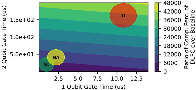
Figure 8: Evaluation of dlpc across machines. The contour plots the ratio of the compilation percentage of dlpc to the baseline approach as a function of gate times. Compilation percentage is given by compilation time over total execution time. A small number on the contour indicates that the baseline approach spent a large portion of its runtime compiling relative to dlpc. The figure indicates typical runtimes of superconducting (SC) [22], neutral atom (NA) [12] and trapped-ion (TI) [3] systems, with TI systems demonstrating the least advantage and SC the most.

VII-B Beyond qci Routines

While primarily motivated by qci problems, dlpc can also be extended to non-qci programs as demonstrated in the rb target application. A potential non-qci application of dlpc is quantum computers in the cloud. Most commercial quantum computers are available to users through the cloud [33]. These machines follow a workload management system where users submit their quantum jobs to a queue. Each circuit is first compiled and optimized at the operation level, before being compiled and uploaded to the qpu for execution. However, given that each of the submitted circuits to the queue is targeting the same machine, they have an underlying shared structure of using the same native gate set. This shared structure can be used to extend dlpc to the quantum computing workflow in the cloud.

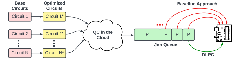
Figure 9: Workflow for quantum computers hosted on the cloud start with users submitting their circuits. These circuits are optimized on the client side before being added to a job queue. The baseline approach compiles the kernel for each of these circuits prior to execution. dlpc re-compiles the kernel only when the jobs in the queue go to zero, or the system needs to recalibrate.

Each circuit submitted to the quantum computer still needs to be compiled and optimized at the circuit level. Once it has been added to the execution queue and reduced to the native gate set, dlpc can be used to save the repeated device-level compilation costs. A simple way to ensure that there is no kernel re-compilation and that all the native gates have been pre-compiled on the system is to run a dummy circuit consisting of all the native gates at the beginning of the queue. Fig 9 summarizes the design of the dlpc technique applied to quantum computers in the cloud.

In Fig 10 we emulate cloud workflow over a day to approximate the cumulative time spent compiling circuits using dlpc. The kernel only recompiles if the number of jobs in the queue go to zero, or the system needs to undergo a re-calibration procedure (considered to be every 2 hours). We demonstrate results for 12000 circuits a day with varying workflow distributions through the course of a day and varying circuit sizes. Small circuits result in the largest cumulative kernel compilation time ($\sim$40.7 on minutes on average across distributions) as the jobs in the queue are executed quickly, resulting in the queue going to zero routinely. For large circuits, long execution times result in the kernel being recompiled only for periodic re-calibration leading to a minimal compilation cost. In contrast, the baseline approach recompiles the kernel for each circuit resulting in a cumulative average compilation time of $\sim$2.7 hours over the a day.

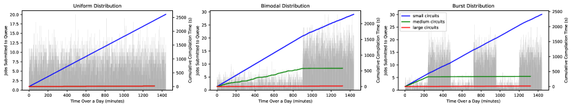
Figure 10: Cumulative kernel compilation time for dlpc over a day across 3 distributions - uniform, bimodal and burst; and 3 circuit sizes - small ($\sim$30 gates), medium ($\sim$100 gates) and large ($\sim$200 gates). In comparison, the baseline approach re-compiles for each circuit resulting in cumulative compilation cost of $\sim$2.7 hours over a day.

VIII Re-optimization and Re-calibration

In prior sections, we have assumed that both changes in circuit parameters does not require a re-optimization of the resulting circuit and device drift is insignificant. In both cases, this advantages DLPC because the compiled information in the kernel is assumed perfect. In practice, neither is a reasonable assumption; changes in gate parameters can possibly be optimized as they change and device parameters can drift resulting in stale device level instructions.

VIII-A Circuit Re-optimization

Changes in gate parameters, such as rotation angles, do not often result in significant structural changes in the circuit, even with a complete circuit-level re-transpilation. If error rate drifts could be accurately predicted, high level circuit optimization could dynamically remap programs onto less error prone qubits; no such accurate prediction exists today.

In typical vqe programs, re-optimizing and re-compiling the circuit between iterations results in some gate count and circuit duration changes. These changes, however, are due to non-determinism in mapping and routing algorithms and not because of significant circuit re-optimization. If the transpilation is seeded, these variations vanish. Frequent exits out of the host-kernel loop are largely unnecessary, and instead, it is more favorable to highly optimize the original parameterized circuit and then require only a single kernel compilation. In some implementations of variational algorithms, for example ADAPT-VQE [14], the circuit structure itself is a variational parameter and different circuit substructures are added at each iteration. Circuit re-optimization could result in significantly reduced depth or gate count, both the primary sources of error. Often these components are small and re-optimizing every iteration is unnecessary because few gate cancellations are expected. It is more practical to periodically force re-optimization of the circuit which will also require a recompilation of the kernel, while still avoiding re-compilation at each iteration. If there are significant circuit changes warranting re-optimzations every iteration, dlpc would still accommodate this due to the underlying shared structure of the native gate set (see Sec. VII-B).

VIII-B Hardware Drift

Device parameters are known to drift over time, resulting in calibration information becoming stale and increasing error rates [31]. Parameters are frequently updated after rounds of calibration. Both the circuit and the kernel should be recompiled to account for a potentially new device error landscape.

Because drift is not uniform it can be unnecessarily expensive to re-calibrate the entire system, calibrating both parameters that have remained “in-spec” as well as those which have fallen “out-of-spec.” To accommodate this, more flexible and dynamic calibration schemes have emerged, such as Optimus [20], which constructs a calibration dependency graph which is periodically probed to determine which parameters to re-calibrate. Low shot-count overhead probes can be used to determine what has drifted out-of-spec. The size of this graph should scale quadratically with the number of qubits in a system with all-to-all connectivity.

Even when done quickly [41], 10-15 experiments per node in the Optimus graph can lead to excessive kernel compilation overheads, increasing with the rate of drift which determines the frequency nodes will fail their probes. Following from [34], we construct sparse random Optimus graphs with various failure rates for each node. We select random nodes as the starting point and follow the Optimus algorithm and use the expected calibration times reported in [41] for both the number of experiments (number of times kernel compilation is executed in the baseline case) and the time to complete these experiments. dlpc avoids kernel re-compilation for calibration routines. We estimate probe execution time to be an order of magnitude cheaper, though the exact cost of these probes is not specified in either prior works [34, 20]. The goal of this experiment is to demonstrate how drift can be both probed and corrected dynamically, however with potentially large overhead which is reduced by integrating DLPC. The accommodation of Optimus in dlpc is summarized in Fig 11.

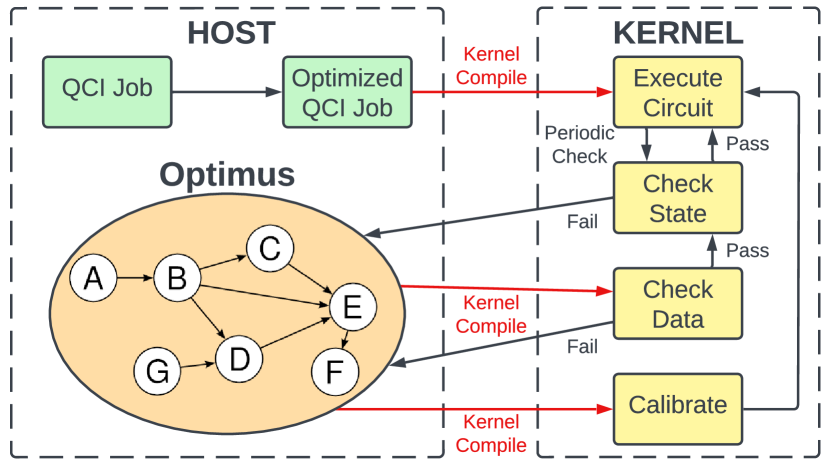
Figure 11: Optimus is a flexible, graph-based re-calibration routine which periodically checks hardware parameters and re-calibrates those which have fallen “out of spec.” However, in the baseline case these routines require kernel compilation to run the system probes (check data) and the calibration procedure apart from compiling the circuit kernel. We indicate these kernel compilations in red. When using the baseline approach each of these kernel compilations are repeated depending on the number of system probes, and size of the calibration graph in addition to multiple circuit runs. dlpc reduces these kernel compilations for Optimus and circuit execution.

In Fig 12, we compare various schemes including periodic forced recalibration of each routine in the Optimus graph (here it is infrequent, hence lower than the Optimus approach with fast drift), forced circuit optimization, and the generalized Optimus approach with random probes at various drift rates. Compared to the non-calibration versions of either naive or DLPC, these will necessarily be more expensive. However, notably DLPC has significant reductions in kernel compilation times, specifically due to the integrated probe and calibration routines. In this experiment, we explore a small qubit VQE instance (5 qubits) to solve for a single bond angle with several hundred iterations and with shot counts approximated by [5, 11, 15] (order of thousands per iteration). Because of the random query model, we report the average over hundreds of samples. With DLPC, both the total execution time and the fraction of time spent compiling the kernel is substantially smaller compared to the baseline implementation. Because the underlying circuit is small, circuit reoptimization takes a very small fraction of the total runtime.

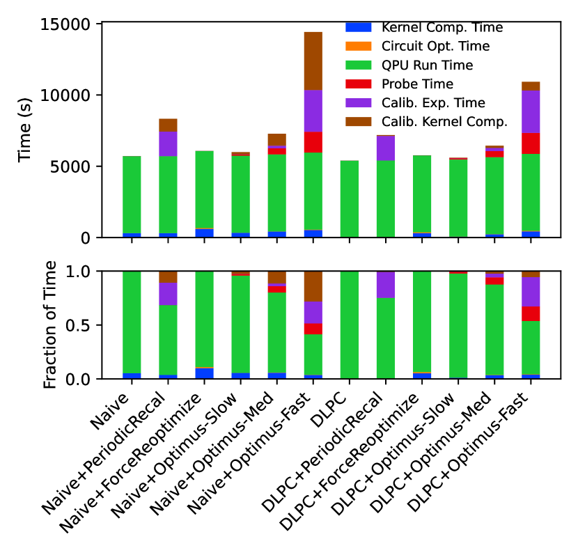
Figure 12: Execution time of activities when running under different calibration and optimization routines, both without (Naive) and with DLPC. Here VQE runs with hundreds of iterations each with 1000 shots. After each iteration we randomly query an Optimus graph (as in [34]) which probabilistically reports failure relative to the drift rate. On failures, we run calibration of the node using experiment counts and execution times reported from [41]. As drift increases, both the time spent calibrating and the total number of experiments, hence kernel compilations, increases. With DLPC we remain in the kernel and accommodate dynamic re-calibration, reducing the total fraction (bottom) of time spent doing classical tasks.

IX Related Work

Compilation of quantum programs has been studied extensively, though primarily at the circuit and pulse level. In [9], they explore the use of partial compilation at the pulse level by dividing the circuit structure into blocks which either are or are not re-compiled into pulses every iteration. Regardless of which block, the resulting pulses must still then be converted to basic waveforms and machine code to be played out by the control hardware. Our work enables this, extending partial compilation to machine code. Circuit parameterization is not entirely new, for example it is currently part of the OpenQASM 3.0 [6] spec, however these are entirely high-level representations, not executable instructions and must be converted into hardware-specific executables. The quantum-classical interfacing problem has also been explored before, for example with IBM’s Qiskit Runtime [32], which enables users to submit entire jobs with interleaved classical processing rather than just circuits. This is primarily focused on reducing the queue time overheads between individual iteration executions for a single contiguous hardware allocation. However, this does not address the problem of kernel startup or compilation to classical control signals. Our work complements each of these prior works by addressing compilation lower in the pipeline.

X Conclusion

While most current architectural work for quantum computers has focused on high-level machine and pulse optimizations, device-level code optimization has remained largely untouched meaning naive implementations of pulse-to-hardware instruction translation results in unnecessary compilation overhead. This work proposes a dlpc technique that takes advantage of the shared structure and kernel-level invariants of quantum operations. This allows the device-level machine code to be compiled only once, with the changing parameters passed into the binary file through cheap rpc. This technique results in the reduction of compilation overhead for the class of qci problems, as they have a parameterized quantum program that run repeatedly with changing parameters. The technique can also be extended to iterative quantum programs that do not require any interleaved classical input but do have a shared program structure across runs.

We demonstrate this technique on a trapped-ion system and in simulation. We ran simple single-qubit vqe programs on the hardware for a speedup of up to 2.7x using dlpc. We demonstrated dlpc on multi-qubit systems by running optimal pulse calibration routine in simulation and get a runtime speedup of up to 7.7x. We also demonstrate dlpc for system characterization routine rb and see a runtime speedup of up to 2.6x. We evaluate it on other platforms, quantum computing workflow in the cloud, and in cases requiring re-optimization and re-calibration. Our proposed technique is most beneficial on a subset of qci problems where a large number of circuits need to be run for a small number of shots. This is due to the growing domination of circuit execution time over compilation time as the number of shots increases. However, with faster gate times and improved shot budget requirements, the advantage presented by dlpc will grow.

References

- [1] R. Blume-Kohout, J. K. Gamble, E. Nielsen, J. Mizrahi, J. D. Sterk, and P. Maunz, “Robust, self-consistent, closed-form tomography of quantum logic gates on a trapped ion qubit,” 2013. [Online]. Available: https://arxiv.org/abs/1310.4492
- [2] S. Bourdeauducq, R. Jördens, P. Zotov, J. Britton, D. Slichter, D. Leibrandt, D. Allcock, A. Hankin, F. Kermarrec, Y. Sionneau, R. Srinivas, T. R. Tan, and J. Bohnet, “Artiq 1.0,” May 2016. [Online]. Available: https://doi.org/10.5281/zenodo.51303
- [3] C. D. Bruzewicz, J. Chiaverini, R. McConnell, and J. M. Sage, “Trapped-ion quantum computing: Progress and challenges,” Applied Physics Reviews, vol. 6, no. 2, p. 021314, jun 2019. [Online]. Available: https://doi.org/10.1063%2F1.5088164
- [4] F. T. Chong, D. Franklin, and M. Martonosi, “Programming languages and compiler design for realistic quantum hardware,” Nature, vol. 549, no. 7671, pp. 180–187, 2017.
- [5] D. Claudino, J. Wright, A. J. McCaskey, and T. S. Humble, “Benchmarking adaptive variational quantum eigensolvers,” Frontiers in Chemistry, vol. 8, p. 606863, 2020.
- [6] A. Cross, A. Javadi-Abhari, T. Alexander, N. De Beaudrap, L. S. Bishop, S. Heidel, C. A. Ryan, P. Sivarajah, J. Smolin, J. M. Gambetta, and B. R. Johnson, “Openqasm 3: A broader and deeper quantum assembly language,” ACM Transactions on Quantum Computing, vol. 3, no. 3, sep 2022. [Online]. Available: https://doi.org/10.1145/3505636
- [7] M. L. Dahlhauser and T. S. Humble, “Benchmarking characterization methods for noisy quantum circuits,” 2022.
- [8] A. Erhard, J. J. Wallman, L. Postler, M. Meth, R. Stricker, E. A. Martinez, P. Schindler, T. Monz, J. Emerson, and R. Blatt, “Characterizing large-scale quantum computers via cycle benchmarking,” Nature Communications, vol. 10, no. 1, p. 5347, Nov 2019. [Online]. Available: https://doi.org/10.1038/s41467-019-13068-7
- [9] P. Gokhale, Y. Ding, T. Propson, C. Winkler, N. Leung, Y. Shi, D. I. Schuster, H. Hoffmann, and F. T. Chong, “Partial compilation of variational algorithms for noisy intermediate-scale quantum machines,” in Proceedings of the 52nd Annual IEEE/ACM International Symposium on Microarchitecture, ser. MICRO ’52. New York, NY, USA: Association for Computing Machinery, 2019, p. 266–278. [Online]. Available: https://doi.org/10.1145/3352460.3358313
- [10] J. F. Gonthier, M. D. Radin, C. Buda, E. J. Doskocil, C. M. Abuan, and J. Romero, “Measurements as a roadblock to near-term practical quantum advantage in chemistry: Resource analysis,” Physical Review Research, vol. 4, no. 3, aug 2022. [Online]. Available: https://doi.org/10.1103%2Fphysrevresearch.4.033154
- [11] J. F. Gonthier, M. D. Radin, C. Buda, E. J. Doskocil, C. M. Abuan, and J. Romero, “Measurements as a roadblock to near-term practical quantum advantage in chemistry: resource analysis,” Physical Review Research, vol. 4, no. 3, p. 033154, 2022.
- [12] T. M. Graham, Y. Song, J. Scott, C. Poole, L. Phuttitarn, K. Jooya, P. Eichler, X. Jiang, A. Marra, B. Grinkemeyer, M. Kwon, M. Ebert, J. Cherek, M. T. Lichtman, M. Gillette, J. Gilbert, D. Bowman, T. Ballance, C. Campbell, E. D. Dahl, O. Crawford, N. S. Blunt, B. Rogers, T. Noel, and M. Saffman, “Multi-qubit entanglement and algorithms on a neutral-atom quantum computer,” Nature, vol. 604, no. 7906, pp. 457–462, Apr 2022. [Online]. Available: https://doi.org/10.1038/s41586-022-04603-6
- [13] D. J. Griffiths and D. F. Schroeter, Introduction to Quantum Mechanics, 3rd ed. Cambridge University Press, 2018.
- [14] H. R. Grimsley, S. E. Economou, E. Barnes, and N. J. Mayhall, “An adaptive variational algorithm for exact molecular simulations on a quantum computer,” Nature Communications, vol. 10, no. 1, p. 3007, Jul 2019. [Online]. Available: https://doi.org/10.1038/s41467-019-10988-2
- [15] A. Gu, A. Lowe, P. A. Dub, P. J. Coles, and A. Arrasmith, “Adaptive shot allocation for fast convergence in variational quantum algorithms,” 2021. [Online]. Available: https://arxiv.org/abs/2108.10434
- [16] R. S. Gupta, L. C. G. Govia, and M. J. Biercuk, “Integration of spectator qubits into quantum computer architectures for hardware tune-up and calibration,” Phys. Rev. A, vol. 102, p. 042611, Oct 2020. [Online]. Available: https://link.aps.org/doi/10.1103/PhysRevA.102.042611
- [17] S. Hadfield, Z. Wang, B. O’gorman, E. G. Rieffel, D. Venturelli, and R. Biswas, “From the quantum approximate optimization algorithm to a quantum alternating operator ansatz,” Algorithms, vol. 12, no. 2, p. 34, 2019.
- [18] J. Helsen, X. Xue, L. M. K. Vandersypen, and S. Wehner, “A new class of efficient randomized benchmarking protocols,” npj Quantum Information, vol. 5, no. 1, p. 71, Aug 2019. [Online]. Available: https://doi.org/10.1038/s41534-019-0182-7
- [19] G. Kasprowicz, P. Kulik, M. Gaska, T. Przywozki, K. Pozniak, J. Jarosinski, J. W. Britton, T. Harty, C. Balance, W. Zhang, D. Nadlinger, D. Slichter, D. Allcock, S. Bourdeauducq, R. Jördens, and K. Pozniak, “Artiq and sinara: Open software and hardware stacks for quantum physics,” in OSA Quantum 2.0 Conference. Optical Society of America, 2020, p. QTu8B.14. [Online]. Available: http://www.osapublishing.org/abstract.cfm?URI=QUANTUM-2020-QTu8B.14
- [20] J. Kelly, P. O’Malley, M. Neeley, H. Neven, and J. M. Martinis, “Physical qubit calibration on a directed acyclic graph,” arXiv preprint arXiv:1803.03226, 2018.
- [21] J. Kim, T. Chen, J. Whitlow, S. Phiri, B. Bondurant, M. Kuzyk, S. Crain, K. Brown, and J. Kim, “Hardware design of a trapped-ion quantum computer for software-tailored architecture for quantum co-design (staq) project,” in Quantum 2.0. Optical Society of America, 2020, pp. QM6A–2.
- [22] Y. Kim, A. Eddins, S. Anand, K. X. Wei, E. van den Berg, S. Rosenblatt, H. Nayfeh, Y. Wu, M. Zaletel, K. Temme, and A. Kandala, “Evidence for the utility of quantum computing before fault tolerance,” Nature, vol. 618, no. 7965, pp. 500–505, Jun 2023. [Online]. Available: https://doi.org/10.1038/s41586-023-06096-3
- [23] E. Knill, D. Leibfried, R. Reichle, J. Britton, R. B. Blakestad, J. D. Jost, C. Langer, R. Ozeri, S. Seidelin, and D. J. Wineland, “Randomized benchmarking of quantum gates,” Phys. Rev. A, vol. 77, p. 012307, Jan 2008. [Online]. Available: https://link.aps.org/doi/10.1103/PhysRevA.77.012307
- [24] E. Magesan, J. M. Gambetta, and J. Emerson, “Scalable and robust randomized benchmarking of quantum processes,” Physical review letters, vol. 106, no. 18, p. 180504, 2011.
- [25] S. Majumder, L. Andreta de Castro, and K. R. Brown, “Real-time calibration with spectator qubits,” npj Quantum Information, vol. 6, no. 1, p. 19, Feb 2020. [Online]. Available: https://doi.org/10.1038/s41534-020-0251-y
- [26] A. Maksymov, P. Niroula, and Y. Nam, “Optimal calibration of gates in trapped-ion quantum computers,” Quantum Science and Technology, vol. 6, no. 3, p. 034009, jun 2021. [Online]. Available: https://dx.doi.org/10.1088/2058-9565/abf718
- [27] H. Neven, J. Martinis, J. Kelly, M. Neeley, and P. J. J. O’Malley, “Physical qubit calibration on a directed acyclic graph,” arXiv, possibly npj Quantum Information, 2018.
- [28] T. Nguyen, A. Santana, T. Kharazi, D. Claudino, H. Finkel, and A. McCaskey, “Extending c++ for heterogeneous quantum-classical computing,” arXiv preprint arXiv:2010.03935, 2020.
- [29] A. Peruzzo, J. McClean, P. Shadbolt, M.-H. Yung, X.-Q. Zhou, P. J. Love, A. Aspuru-Guzik, and J. L. O’Brien, “A variational eigenvalue solver on a photonic quantum processor,” Nature Communications, vol. 5, no. 1, p. 4213, Jul 2014. [Online]. Available: https://doi.org/10.1038/ncomms5213
- [30] J. Preskill, “Quantum computing in the nisq era and beyond,” Quantum, vol. 2, p. 79, 2018.
- [31] T. Proctor, M. Revelle, E. Nielsen, K. Rudinger, D. Lobser, P. Maunz, R. Blume-Kohout, and K. Young, “Detecting and tracking drift in quantum information processors,” Nature communications, vol. 11, no. 1, p. 5396, 2020.
- [32] Qiskit contributors, “Qiskit: An open-source framework for quantum computing,” 2023.
- [33] G. S. Ravi, K. N. Smith, P. Gokhale, and F. T. Chong, “Quantum computing in the cloud: Analyzing job and machine characteristics,” 2022.
- [34] L. Riesebos, B. Bondurant, and K. R. Brown, “Universal graph-based scheduling for quantum systems,” IEEE Micro, vol. 41, no. 5, pp. 57–65, 2021.
- [35] L. Riesebos, B. Bondurant, J. Whitlow, J. Kim, M. Kuzyk, T. Chen, S. Phiri, Y. Wang, C. Fang, A. V. Horn, J. Kim, and K. R. Brown, “Modular software for real-time quantum control systems,” in 2022 IEEE International Conference on Quantum Computing and Engineering (QCE), 2022, pp. 545–555.
- [36] L. Riesebos and K. R. Brown, “Functional simulation of real-time quantum control software,” in 2022 IEEE International Conference on Quantum Computing and Engineering (QCE), 2022, pp. 535–544.
- [37] L. Riesebos, X. Fu, A. Moueddenne, L. Lao, S. Varsamopoulos, I. Ashraf, J. Van Someren, N. Khammassi, C. G. Almudever, and K. Bertels, “Quantum accelerated computer architectures,” in 2019 IEEE International Symposium on Circuits and Systems (ISCAS), 2019, pp. 1–4.
- [38] V. M. Schäfer, C. J. Ballance, K. Thirumalai, L. J. Stephenson, T. G. Ballance, A. M. Steane, and D. M. Lucas, “Fast quantum logic gates with trapped-ion qubits,” Nature, vol. 555, no. 7694, pp. 75–78, Mar 2018. [Online]. Available: https://doi.org/10.1038/nature25737
- [39] T. M. Stace, J. Chen, L. Li, V. S. Perunicic, A. R. R. Carvalho, M. R. Hush, C. H. Valahu, T. R. Tan, and M. J. Biercuk, “Optimised bayesian system identification in quantum devices,” 2022.
- [40] K. M. Svore, A. V. Aho, A. W. Cross, I. Chuang, and I. L. Markov, “A layered software architecture for quantum computing design tools,” Computer, vol. 39, no. 1, pp. 74–83, 2006.
- [41] C. Tornow, N. Kanazawa, W. E. Shanks, and D. J. Egger, “Minimum quantum run-time characterization and calibration via restless measurements with dynamic repetition rates,” Physical Review Applied, vol. 17, no. 6, p. 064061, 2022.