On the accuracy of interpolation based on single-layer artificial neural networks

Abstract

Artificial Neural Networks (ANNs) are a tool in approximation theory widely used to solve interpolation problems. In fact, ANNs can be assimilated to functions since they take an input and return an output. The structure of the specifically adopted network determines the underlying approximation space, while the form of the function is selected by fixing the parameters of the network. In the present paper, we consider one-hidden layer ANNs with a feedforward architecture, also referred to as shallow or two-layer networks, so that the structure is determined by the number and types of neurons. The determination of the parameters that define the function, called training, is done via the resolution of the approximation problem, so by imposing the interpolation through a set of specific nodes. We present the case where the parameters are trained using a procedure that is referred to as Extreme Learning Machine (ELM) that leads to a linear interpolation problem. In such hypotheses, the existence of an ANN interpolating function is guaranteed.
The focus is then on the accuracy of the interpolation outside of the given sampling interpolation nodes when they are the equispaced, the Chebychev, and the randomly selected ones. We obtain good accuracy of the ANN interpolating function in all tested cases using these different types of interpolating nodes and different types of neurons. The study is motivated by the well-known bell-shaped Runge example, which makes it clear that the construction of a global interpolating polynomial is accurate only if trained on suitably chosen nodes, ad example the Chebychev ones. In order to evaluate the behavior when growing the number of interpolation nodes, we raise the number of neurons in our network and compare it with the interpolating polynomial. We test using Runge’s function and other well-known examples with different regularities. As expected, the accuracy of the approximation with a global polynomial increases only if the Chebychev nodes are considered. Instead, the error for the ANN interpolating function always decays and in most cases we observe that the convergence follows what is observed in the polynomial case on Chebychev nodes, despite the set of nodes used for training.
Our results show the power of ANNs to achieve excellent approximations when interpolating regular functions also starting from uniform and random nodes, particularly for Runge’s function.
Keywords: Feedforward Neural Networks; Function approximation; Runge’s function; Extreme Learning Machine
Subclass 65D05

1 Introduction

With no doubt, Artificial Neural Networks (ANNs) are a numerical analysis tool with a great versatility and, therefore, they have had a great development in recent years [17, 27, 14]. ANNs are a class of machine learning algorithms that have a well-established structure, flexibility, and approximation properties. For this reason, they are widely used for function approximations, classification, regression, feature selection, and further applications are constantly being explored. Nevertheless, they are often considered as a black-box for its complex and nonlinear structure. Moreover, ANNs have open issues on some aspects of efficiency and accuracy when the number of training parameters increases. Furthermore, ANNs have opened the road to Artificial Intelligence with the possibility to develop Digital Twins when a warehouse of input-output data is available, even in cases where the governing laws are unknown, even up to being able to mimic extremely complex phenomena, such as brain reaction.

Of all the highlighted points, the present contribution focuses on the aspect that ANNs can be profitably used in function approximation due to the Universal Approximation (UA) results, even under very mild hypotheses see, e.g., [24]. In particular, UA states that ANNs can approximate a target function with any required precision, i.e., it can be defined an ANN that is close enough to any target function (at least asymptotically) also in spaces endorsed with very low regularity.

Moreover, some ANNs avoid the phenomenon called curse of dimensionality, an expression coined by [4], referring to a set of issues that appears when dealing with high-dimensional data, that are not present when working on low-dimensional problems. For instance, the amount of data needed to obtain a sufficiently good representation of a given domain often increases exponentially with the dimension of the data. The fact that ANNs avoid the curse of dimensionality opens the possibility to achieve efficient approximations, even in high dimensional cases see, e.g., [16, 21, 22, 23, 26].

The construction of ANNs involves the determination of a sufficiently large number of functions (referred to in this context as activation functions) connected in a grid structure composed by nodes. The activation functions and the interactions among nodes are defined with parameters, which are determined via conditions that are intended as an interpolation (or approximation) of the available information. This process is called the training of the network and this is done by tuning the parameters. The first step to train an ANN is to initialize all the parameters in a proper way and then the tuning is performed, usually via optimization strategies, such as the minimization of a so-called loss function see, e.g., [5, 11].

The existence of a “good” interpolation network is guaranteed by the UA results and the large number of available tuning parameters. Such a network can then “remember” the information with which it has been trained and, even more important, is able to give an appropriate answer to new cases, which had not been used on the training process. Translated into mathematical approximation theory language, a trained network is capable to do usual interpolation and extrapolation procedures. On the other hand, from the authors’ point of view, one of the main drawbacks of such a procedure is related to the unclear mathematical interpretation of the underlying approximating space and the definition of the training procedure in presence of a (quasi-) optimal set of parameters [36, 14].

A well known issue in approximation theory is the poor behavior of the degree-increasing polynomial interpolation when applied on some specific functions. In particular, a paradigmatic example of this poor behavior is Runge’s function see, e.g., [10]; when taking uniformly or randomly distributed sampling points of Runge’s function and performing a polynomial interpolation, the difference between approximating and target function outside from the sampling points can diverge as the polynomial order increases. One way to avoid this divergence is to sample the function using ad-hoc nodes, such as Chebychev nodes. However, in many real-world, non theoretical problems ad-hoc optimal sampling cannot be performed, either because data are already given, or because the analytical expression of the underlying function is unknown, or a combination of both.

According to the previous discussion, the main aim of the present paper is to give some insight into the ability of ANNs to approximate functions. We report results for the Runge’s function and, by following examples in [35], also for other benchmark functions that exhibit different regularities. Our reference method is the polynomial approximation obtained by interpolation in Chebychev nodes, as extensively discussed in [35]; such a method is well suited to achieve high degree approximation, as well as for its relationships to the truncation (or projection) of the Chebychev series, and it is widely used also in other applications, such as in numerical quadrature see, e.g. [34, 8]. Moreover, a stable reference implementation is available via CHEBFUN routines in MATLAB [3, 12], so that the comparison can be easily conducted.

The paper is organized as follows. Section 2 presents an introduction to ANNs focusing on the definitions of the main concepts and reviewing available results, with a focus on the properties related to the interpolation. In particular, we set the specific ANN structure, later adopted in the paper, namely a single hidden layer network, trained via Extreme Learning Machine with over-parametrization and solved by Least Squares. In Section 3 we show numerical results. First, we use Runge’s function, where we also report results in the square (not overparametrized) case and for which we evaluate both the approximation of the function and of the derivative, being the derivative of the ANN interpolating function trivial to compute. The section continues with the results relative to other examples taken from Trefethen ([35]), using overparametrized networks and focusing on the approximation of the interpolated functions. Lastly, in Section 4 we present the final thoughts, conclusions and possible future directions.

2 Preliminaries on Neural Networks

In this section we define the main concepts related to Artificial Neural Networks (ANNs). An ANN is a set of connected nodes, usually called neurons, where each neuron takes different real-valued inputs and produces a real-valued output. ANNs may have different connection structures between the neurons, called the architecture of the ANN; for instance, common architectures are: feedforward, deep feedforward, perceptron, convolutional, recurrent, autoencoder, fully complex. In the present work, we consider the most common architecture: the feedforward network (FFN), described in Section 2.1.

The process that each neuron performs is mainly divided into two steps, with each single step being represented by a function. The first step is called interaction scheme and combines the multiple inputs received from the neurons to produce a scalar output. In Section 2.2 we describe some of the possible choices for the interaction scheme. Then, the second step is represented by a transfer function, usually called activation function, which takes the output of the interaction scheme as an input and generates another real value, that is the output of the neuron itself: in Section 2.3 we describe some of the possible choices for the activation functions. The interaction scheme determines how the information coming from a set of inputs is combined, whereas the activation function modulates the result. As discussed in more detail in the respective sections, the choice of each of these steps determines the behavior of the ANN.

After these introductions of ANNs, in Section 2.4 we focus the analysis and particularise the equations to the case of a single hidden layer. Finally, in Section 2.5 we explain the adopted training procedure, called Extreme Learning Machine (ELM).

Throughout the paper we use the following notation. Scalar values are represented by letters without underlining, whereas vectors and matrices are indicated with a single or a double underline, respectively. The elements of a vector are represented with the same letter as the vector itself, with a single sub-script indicating the number of elements. Similarly, the elements of a matrix are represented with the same letter as the matrix itself, using two sub-scripts. In both cases, the letter with the sub-script(s) is not underlined, since it corresponds to a scalar value. Moreover, a single row or column of a matrix (hence a vector) is denoted with the same letter as the matrix and a single sub-script. In this case, the row or column is underlined with a single line since it corresponds to a vector. Finally, super-scripts between parentheses always indicate the corresponding layer number within the ANN.

2.1 Architecture of AANs: the feedforward case

The first choice for the determination of the structure of an ANN is the architecture of the grid. We use the so-called feedforward architecture, resulting in the feedforward network (FFN), where neurons are stored in consecutive layers; the layers are indicated with an index $l$, with $l=0,1,\dots,\mathcal{L},\mathcal{L}+1$. The FFN architecture is such that at each layer the input is taken from the output of the previous layer, elaborated by the interaction scheme and the activation functions of the neurons present in the considered layer, and passed as an input to the next layer. The first layer of the FFN ($l=0$) is called ANN input layer or simply input layer and it is not actually composed by neurons; each unit of this first layer has the only role of reading the input data and to feed them to the following layer of neurons to start the network process; accordingly, the amount of units in the first layer is always equal to the number of inputs of the network. The last layer of the FFN ($l=\mathcal{L}+1$) is called ANN output layer or simply output layer since its neurons’ outputs constitute the output of the network itself. All the layers between the ANN input and output layers ($l=1,\dots,\mathcal{L}$) are called hidden layers. Each $l$–th layer consist of $N^{(l)}$ neurons, each one with its own real scalar output. The set of output values of the $l$–th layer’s neurons can be thus thought as a vector, arranged, for example, in the form: $\underline{x}^{(l)}=(x_{1}^{(l)},\dots,x_{N^{(l)}}^{(l)})\in\mathbb{R}^{N^{(l)}}$. In the FFN architecture, each neuron of the $l$–th layer is fully connected with the nodes of the previous $(l-1)$–th layer by weighted edges (often called just weights); the weights are scalar values associated to the connection between neurons of adjacent layers.

When the network has two or more hidden layers ($\mathcal{L}\geq 2$), the architecture is usually referred to as deep feedforward network (DFFN). Instead, when the network has just one hidden layer ($\mathcal{L}=1$), the architecture is usually referred to as non-deep FFN, or shallow neural networks [29, 33] or two-layer networks [13, 32]. This last terminology evidences the fact that the input layer does not perform any operation, hence such ANN relies only on a single hidden layer and the output layer.

2.2 Interaction schemes

The first step performed by the neurons of the generic $l$–th layer is represented by the interaction scheme, which combines all the outputs of the neurons of the previous layer (i.e. the real values $x_{j}^{(l-1)}$, with $j=1\dots N^{(l-1)}$) to produce a single output value for each single neuron (i.e., the real values denoted in the following as $z_{i}^{(l)}$, with $i=1\dots N^{(l)}$).

For each $i$–th neuron on the $l$–th layer, such a combination of the output neurons of the previous layer is based on the use of a vector of weights, indicated as $\underline{A}_{i}^{(l)}\in\mathbb{R}^{N^{(l-1)}}$, and a scalar bias, indicated as $\beta_{i}^{(l)}\in\mathbb{R}$, with $i=1\dots N^{(l)}$. In general, the interaction scheme of the single neuron is represented as a function $\kappa_{i}^{(l)}:(\underline{x}^{(l-1)},\underline{A}_{i}^{(l)},\beta_{i}^{(l)})\in\mathbb{R}^{N^{(l-1)}}\times\mathbb{R}^{N^{(l-1)}}\times\mathbb{R}\rightarrow z_{i}^{(l)}\in\mathbb{R}$, with $i=1\dots N^{(l)}$, so that:

$$z_{i}^{(l)}=\kappa_{i}^{(l)}(\underline{x}^{(l-1)},\underline{A}_{i}^{(l)},\beta_{i}^{(l)}).$$ (1)

Figure 1 depicts the interaction scheme of the generic $i$–th neuron on the $l$–th layer (the figure also shows the activation function $\psi_{i}^{(l)}$, which is addressed in Section 2.3).

It is possible to organize the weights $\underline{A}_{i}^{(l)}$ and biases $\beta_{i}^{(l)}$ associated to the $i$–th neuron of the $l$–th layer into a matrix and a vector, respectively. We define the weights matrix $\underline{\underline{A}}^{(l)}\in\mathbb{R}^{N^{(l)}\times N^{(l-1)}}$ by laying the vectors $\underline{A}_{i}^{(l)}$ as rows. Likewise, the vector of biases $\underline{\beta}^{(l)}\in\mathbb{R}^{N^{(l)}}$ is defined organizing the individual biases as a vector. Consequently, $\underline{\underline{A}}^{(l)}$ and $\underline{\beta}^{(l)}$ contain the weights and biases associated to all the neurons of the $l$–th layer.

The interaction scheme distinguishes different classes of FFN formulations. In the following we address only the additive and distance-like schemes, referring to them as classic DFFN and RBF networks, respectively, but it is worthwhile to remark that ANNs have been also extended to many others schemes.

2.2.1 Additive interaction scheme

Such a scheme is based on an additive combination of the weights $\underline{A}_{i}^{(l)}$, biases $\beta_{i}^{(l)}$ and inputs $\underline{x}^{(l-1)}$, and it is defined as follows:

$$z_{i}^{(l)}=\sum_{j=1}^{N^{(l-1)}}A_{ij}^{(l)}x_{j}^{(l-1)}+\beta_{i}^{(l)}\qquad i=1,\dots,N^{(l)},$$ (2)

where $A_{ij}^{(l)}$ is the $i$–th row and $j$–th column element of the matrix $\underline{\underline{A}}^{(l)}$.

2.2.2 Distance-like interaction scheme

Such a scheme is based on the extension of the notion of Radial Basis Functions (RBF) to the networks and it is defined as follows.

$$z_{i}^{(l)}=\frac{||\underline{x}^{(l-1)}-\underline{A}_{i}^{(l)}||_{2}}{\beta_{i}^{(l)}}\qquad i=1,\dots,N^{(l)},$$ (3)

where $\underline{A}_{i}^{(l)}$ is the $i$–th row of the matrix $\underline{\underline{A}}^{(l)}$.

Since internal parameters $(\underline{A}_{i}^{(l)},\beta_{i}^{(l)})$ are difficult to train, one common choice is to fix the radius $\beta_{i}^{(l)}$ and set random centers $\underline{A}_{i}^{(l)}$ and then proceed to the solution of the linear system in the weights of the last layer $\underline{A}_{i}^{(\mathcal{L}+1)}$ see, e.g., [7, 19]. Such a procedure is similar to the one proposed in the training via ELMs, as we present in Section 2.5.

2.3 Activation functions

The second step performed by each neuron in the $l$–th layer is to modulate the output of the interaction scheme $z_{i}^{(l)}$ by means of the activation function to produce the so-called output of the neuron, which is indicated as $x_{i}^{(l)}$. The output $x_{i}^{(l)}$ is computed by the activation function $\psi_{i}^{(l)}:z^{(l)}_{i}\in\mathbb{R}\rightarrow x_{i}^{(l)}\in\mathbb{R}$ as:

$$x_{i}^{(l)}=\psi_{i}^{(l)}(z_{i}^{(l)})\qquad i=1,\dots,N^{(l)}.$$ (4)

Figure 1 shows a representation of the action of the generic $i$–th neuron on the $l$–th layer, including both the interaction scheme $\kappa_{i}^{(l)}$ and the activation function $\psi_{i}^{(l)}$.

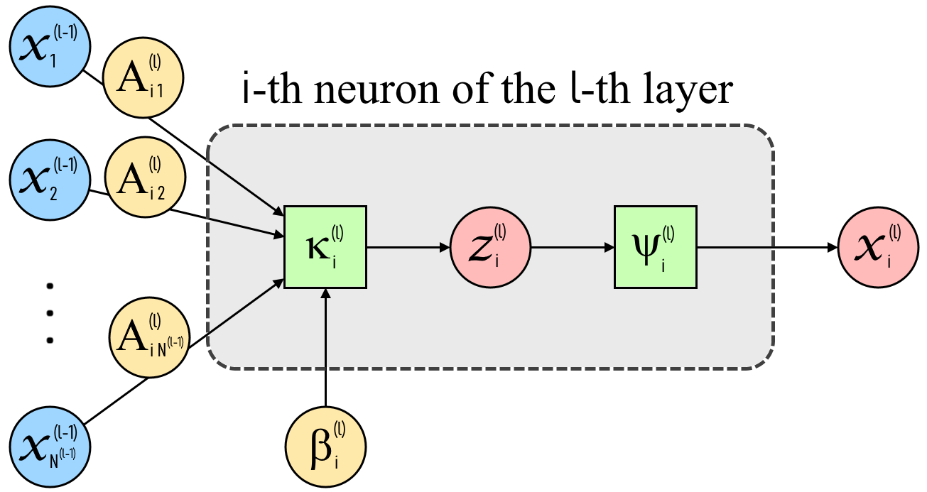
Figure 1: Schematic representation of the action of the generic $i$–th neuron of the $l$–th layer. The inputs $x_{j}^{(l-1)}$ are represented with blue circles, the weights $A_{ij}^{(l)}$ and bias $\beta_{i}^{(l)}$ are represented by yellow circles, the computed values $z_{i}^{(l)}$ and $x_{i}^{(l)}$ are represented with red circles and the functions performed by the neuron (i.e. the interaction scheme $\kappa_{i}^{(l)}$ and the activation function $\psi_{i}^{(l)}$) are represented with green squares.

The use of activation functions gives a wide range of possibilities when defining a network. In principle, one can mix the use of different activation functions in the different hidden layers. However, we use just one activation function for all neurons of all layers, i.e.: $\psi_{i}^{(l)}=\psi$. In the following, we report the choices that are more common and that we consider in our tests.

2.3.1 Activation functions used with additive interaction scheme

The most common choices for activation functions adopted in combination with additive interaction scheme are:

• Logistic Sigmoid (LS):

  $$\psi(x)=\frac{1}{1+\text{exp}(-x)}$$

• SoftPlus (SP):

  $$\psi(x)=\log(1+\text{exp}(x)).$$

LS and SP functions are widely used when performing approximations in unbounded domains or for extrapolating.

Another common activation function adopted in combination with additive interaction scheme is the Rectified Linear Unit (ReLU), which is defined as $\psi(x)=max\{x,0\}$. Notice that the SP function is a smooth $C^{\infty}$ approximation of the ReLU function with the property that the derivative of the SP function is the LS function. It is well known that shallow networks with ReLU activation functions have piece-wise linear functions as an output. Since our aim is to obtain regular functions on the output of the ANN, in our tests we do not implement networks with ReLU activation functions.

Finally, we recall that in the case of shallow networks with LS activation functions the network gives the formation of the so-called Ridge functions [30], or superimpositions of LS functions [2].

2.3.2 Activation functions used with distance-like interaction scheme

A common choice for activation function adopted in combination with distance-like interaction scheme is:

• Gaussian Radial Basis (GRB):

  $$\psi(x)=\text{exp}(-x^{2})$$

GRB functions are widely used in different domains, and the understanding of the properties of these is well established, see e.g. [15].

2.4 Mathematical formulation of the entire ANN

According to the notation presented above, for each ANN layer, we can define a layer map $\underline{\Phi}^{(l)}:\underline{x}^{(l-1)}\in\mathbb{R}^{N^{(l-1)}}\rightarrow\underline{x}^{(l)}\in\mathbb{R}^{N^{(l)}}$ for $l=1,\dots,\mathcal{L}+1$ as:

$$\underline{x}^{(l)}=\underline{\Phi}^{(l)}(\underline{x}^{(l-1)})=\biggl{(}\psi_{1}^{(l)}(z_{1}^{(l)}),\dots,\psi_{N^{(l)}}^{(l)}(z_{N^{(l)}}^{(l)})\biggr{)}\qquad\textnormal{with }z_{i}^{(l)}=\kappa_{i}^{(l)}(\underline{x}^{(l-1)},\underline{A}_{i}^{(l)},\beta_{i}^{(l)})$$ (5)

Finally, the whole ANN can be interpreted as a map $\mathcal{F}:\underline{x}^{(0)}\in\mathbb{R}^{N^{(0)}}\rightarrow\underline{x}^{(\mathcal{L}+1)}\in\mathbb{R}^{N^{(\mathcal{L}+1)}}$, i.e. a map between the input domain and the output domain that can be expressed by:

$$\underline{x}^{(\mathcal{L}+1)}=\mathcal{F}(\underline{x}^{(0)})=\underline{\Phi}^{(\mathcal{L}+1)}\circ\dots\circ\underline{\Phi}^{(1)}(\underline{x}^{(0)})$$ (6)

where the symbol $\circ$ is the function composition, i.e., $f\circ g(x)=f(g(x))$.

When FFNs are used for regression or approximation purposes in the context of continuous, integrable or square-integrable functions, a common choice is to use linear activation functions for the neurons on the last layer. The final output is taken as a linear combination of the evaluations done at the last hidden layer, so that transfer functions of the last layer $\psi_{i}^{(\mathcal{L}+1)}$ are the identity functions:

$$x_{i}^{(\mathcal{L}+1)}=\sum_{j=1}^{N^{(\mathcal{L})}}A^{(\mathcal{L}+1)}_{ij}\psi_{j}^{(\mathcal{L})}(z_{j}^{(\mathcal{L})})\qquad i=1,\dots,N^{(\mathcal{L}+1)}\,.$$ (7)

In this case, the structure of the FFN is exactly a linear combination of the activation functions of the last hidden layer’s neurons. If such functions are chosen linearly independent, they are a basis of the approximating space, so this space is easily described. Overall, the effect of the weights of the last hidden layer is only to combine the activation functions, whereas altering the internal parameters that define the shape of the functions changes the approximating space.

2.4.1 Approximation results

The universal approximation result can be enunciated for FFNs with the same activation function for alla the FFN as follows.

Theorem 2.1

Consider a DFFN with the same activation function $\psi$ in all the neurons of all the layers. Moreover let $\psi\in C(\mathbb{R})$. Then the space $\mathcal{M}^{(\mathcal{L})}(\psi)$ generated by a linear combination of the outputs of the last hidden layer $\underline{x}^{(\mathcal{L})}$, defined by:

$$\mathcal{M}^{(\mathcal{L})}(\psi)=\sum_{i=1}^{N^{(\mathcal{L})}}w_{i}\psi(z_{i}^{(\mathcal{L})})\qquad\textnormal{with }z_{i}^{(\mathcal{L})}=\kappa_{i}^{(\mathcal{L})}(\underline{x}^{(\mathcal{L}-1)},\underline{A}_{i}^{(\mathcal{L})},\beta_{i}^{(\mathcal{L})})$$

is dense in $C(\mathbb{R})$, in the topology of uniform convergence on compacta, if and only if $\psi$ is not a polynomial.

Notice that the choice of the interaction scheme is not discussed here since the two cases presented in Section 2.2 fulfill the requested hypotheses.

We remark that the norm associated to the uniform convergence on compacta is very general, since if $\mu$ is a non–negative finite Borel measure defined on some compact set $K$, then $C(K)$ is dense in $L^{p}(K,\mu)$, for any $1\leq p\leq+\infty$.

The possibility of using different activation functions in different layers comes as a consequence of the universal approximation result, that states that a property on universal approximation can be obtained with every non-polynomial function see, e.g., [25, 18, 28]. In fact, Theorem 2.1 can be easily extended to networks with different activation functions in different layers; assuming to deal with two different activation functions $\psi_{1}$ and $\psi_{2}$ in different layers, then the generated space is the direct sum of two spaces dense in $C(\mathbb{R})$: $\mathcal{M}^{(\mathcal{L})}(\psi_{1},\psi_{2})=\mathcal{M}^{(\mathcal{L})}(\psi_{1})\bigoplus\mathcal{M}^{(\mathcal{L})}(\psi_{2})$. Furthermore, from a density point of view, there is no need to consider a deep ANN, because, at least for the univariate case, a single hidden layer is enough to achieve the universal approximation propriety. Moreover, the construction of deep neural networks gives spaces of composite functions, see (6), and such composition is unnecessary for the interpolation or approximation of univariate functions due to Theorem 2.1.

Furthermore, we would like to point out that such a composition can be interpreted as a construction of a new feature set for the output layer. In fact, when a point $\underline{x}^{(0)}$ is given as an input, this is transformed in an element in the $N^{(1)}$–dimensional space by the action of the activation functions of first hidden layer; then, the activation functions of the second hidden layer - or, in the case of one layer, the activation function - has to deal with the new point $\underline{x}^{(1)}$ and, so on, this happens in all the intermediate layers. Accordingly, one common point of view to look at the behavior of ANNs is to think that the effect of all hidden layers is to encode the input in $N^{(\mathcal{L})}$ new coordinates (i.e., the outputs of the last hidden layer), acting thus as a filter. Then, these $N^{(\mathcal{L})}$ values are linearly combined to give the output, when linear activation functions for the neurons on the last layer are used. In other words, the network takes the input data and converts it into numbers that, linearly combined with a weight vector, determine the behavior of the network.

2.4.2 Single hidden layer FFN in the univariate scalar case

Our aim now is to particularise the formulae from previous sections to the case of a single hidden layer ANN and univariate scalar functions, which are the focus of the present work.

In the case of a single hidden layer ($\mathcal{L}=1$), the FFN is composed only by three layers, numbered $l=0$ (input layer), $l=1$ (hidden layer) and $l=2$ (output layer); then, there are only two matrices of weights $\underline{\underline{A}}^{(1)}$ and $\underline{\underline{A}}^{(2)}$ and two vectors of biases $\underline{\beta}^{(1)}$ and $\underline{\beta}^{(2)}$.

Moreover, when the target functions to be interpolated are univariate and scalar (as we consider in our work), the ANN can be further simplified. On the one hand, the fact that the functions are univariate implies that $N^{(0)}=1$, hence $x^{(0)}$ is a scalar and $\underline{A}^{(1)}$ reduces to a vector. On the other hand, the fact that the functions are scalar implies that $N^{(2)}=1$, hence $x^{(2)}$ and $\beta^{(2)}$ reduce to scalars and $\underline{A}^{(2)}$ reduces to a vector, which we write as: $\underline{A}^{(2)}=\underline{w}=(w_{1},w_{2},\dots,w_{N^{(1)}})\in\mathbb{R}^{N^{(1)}}$ and we denote as external weights. Figure 2 shows a diagram of the resulting ANN.

Under these conditions, equations (6) and (7) become, respectively:

$$\begin{split}&x^{(2)}=\mathcal{F}(x^{(0)})=\Phi^{(2)}(\underline{\Phi}^{(1)}(x^{(0)})),\\ &\textnormal{where }\underline{\Phi}^{(1)}(x^{(0)})=\biggl{(}\psi_{1}^{(1)}(z_{1}^{(1)}),\dots,\psi_{N^{(1)}}^{(1)}(z_{N^{(1)}}^{(1)})\biggr{)}\textnormal{ and }\Phi^{(2)}\equiv\psi^{(2)}\,,\ \end{split}$$ (8)

$$x^{(2)}=\sum_{i=1}^{N^{(1)}}w_{i}\psi_{i}^{(1)}(z_{i}^{(1)})\ \qquad\textnormal{with }z_{i}^{(1)}=\kappa_{i}^{(1)}(x^{(0)},A_{i}^{(1)},\beta_{i}^{(1)}).$$ (9)

A classic FFN with a single hidden layer of $N^{(1)}$ neurons and with an additive interaction scheme can be written as:

$$x^{(2)}=\sum_{i=1}^{N^{(1)}}w_{i}\psi_{i}^{(1)}\biggl{(}A_{i}^{(1)}x^{(0)}+\beta_{i}^{(1)}\biggr{)}\ .$$ (10)

Likewise, a RBF network with a single hidden layer of $N^{(1)}$ neurons can be written as:

$$x^{(2)}=\sum_{i=1}^{N^{(1)}}w_{i}\psi_{i}^{(1)}\biggl{(}\frac{|{x}^{(0)}-{A}_{i}^{(1)}|}{\beta_{i}^{(1)}}\biggr{)}\ .$$ (11)

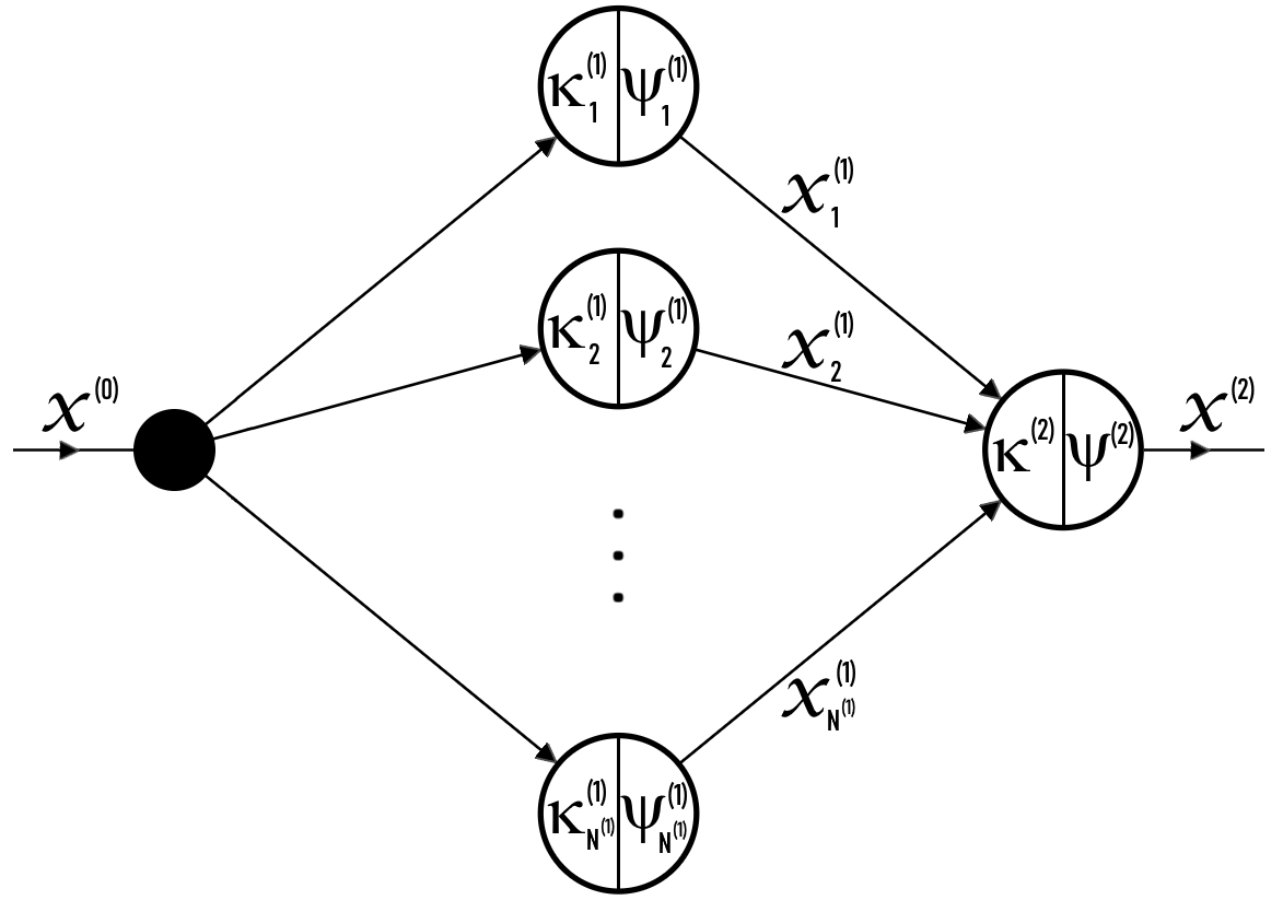
Figure 2: Schematic representation of the single-hidden layer ANN with scalar input $x^{(0)}$ and scalar output $x^{(2)}$. Each neuron is represented by a circle divided into the interaction scheme $\kappa_{i}^{(l)}$ and the activation function $\psi_{i}^{(l)}$. The input neuron, which does not perform any of these operations, is represented by a black dot.

2.5 Training of the single-layer network

When a choice has been done for the number of neurons $N^{(1)}$ and for the activation functions $\psi_{i}^{(1)}$ (see, for example, equations (10) and (11)), then we are left with the determination of the unknown parameters $A_{i}^{(1)}$, $\beta_{i}^{(1)}$ and $w_{i}$, with $i=1\dots N^{(1)}$ (a process often indicated as training process). Among all possible choices, we assume to fix a-priori all weights and biases associated to the neurons in the hidden layer, i.e. $A_{i}^{(1)}$ and $\beta_{i}^{(1)}$, choice often indicated under the name of Extreme Learning Machine (ELM) and the ANNs trained this way are usually called Random Projection Networks. Accordingly, the only unknown of a FFN trained via ELM are the external weights $w_{i}$, i.e. the coefficients of the linear combination of the outputs of the hidden layer. The weights $w_{i}$ are selected throughout the optimization problem, that in our case is the satisfaction of the interpolation requirements.

Therefore, the number of degrees of freedom of an ELM network ($N_{dof}^{ELM}$) is equal to the number of neurons in the last hidden layer, independently of how many hidden layers are considered. In our case:

$$N_{dof}^{ELM}=N^{(1)},$$ (12)

whereas for a generic classical DFFN, with $\mathcal{L}$ hidden layers, the number of degrees of freedom would be $N_{dof}^{DFFN}=N^{(\mathcal{L})}+\sum_{i=0}^{\mathcal{L}-1}(N^{(i)}+1)\cdot N^{(i+1)}$.

Remark: The suggested ELM training procedure, based on a choice made via random selection for part of the unknown parameters and some linear problems to be solved for the determination of the remaining unknown parameters, has been very vastly studied in the literature. When ELM was defined by Huang and co-authors, it gained huge popularity and lead to very interesting developments [20]. Nevertheless, the debate on the original denomination or on the first researcher that has introduced such a procedure populates both scientific papers and internet blogs. In the authors’ opinion, the contribution due to Huang is out of doubt, though it is far from the scope of the authors to crown one scholar or another. We refer to two websites for those who are interested in such debate.

Remark: In the ELM framework, the multilayer construction (i.e., deep ANNs) becomes a linear combination of trial functions, which are, in turn, compositions of activation functions, themselves generated by the random choices of the parameters. The deep architecture is usually adopted when considering high-dimensional problems. However, in our experience, for the low-dimensional approximation problem considered, the structure of the deep network is not necessary to meet the required properties, but is only useful to change the shape of the functions.

2.6 Resulting interpolation problem

Based on the ELM training procedure adopted in the present work, we can define a function $\tilde{u}$ to summarize the action of the entire network (called the network function). The network function relates the network input and the external weights with the network output, such that: $x^{(2)}=\tilde{u}(x^{(0)},\underline{w})$. In our approximation problem, $x^{(0)}$ and $x^{(2)}$ are the independent and dependent variables of the target univariate scalar function sought to be interpolated. The leading philosophy of the ELM framework is to learn only external weights since the following theorem holds see [20]:

Theorem 2.2

Let $(x_{j},y_{j})\,,\ j=1,\dots,M$ be a set of data points such that $x_{j}\not=x_{j+1}$, and lets take the single-layer FFN with $N^{(1)}\leq M$ neurons, then:

$$\tilde{u}(x_{j};w_{i})=\sum_{i=1}^{N^{(1)}}w_{i}\psi_{i}^{(1)}(z_{i}^{(1)})\qquad\textnormal{with}\quad z_{i}^{(1)}=\kappa_{i}^{(1)}(x^{(0)},A_{i}^{(1)},\beta_{i}^{(1)})\,,$$ (13)

Moreover, consider weights $A_{i}^{(1)}$ and bias $\beta^{(1)}$ randomly generated, independently from the data points $(x_{j},y_{j})$, according to any continuous probability distribution $\mathbb{P}$. Then, $\forall\varepsilon>0$, there exists a choice of $\underline{w}$ such that $\mathbb{P}(\|(\tilde{u}(x_{j};w_{i})-y_{j})\|<\varepsilon)=1$. Moreover, if $N^{(1)}=M$ then $w_{i}$ can be found such that $\mathbb{P}(\|(\tilde{u}(x_{j};w_{i})-y_{j})\|=0)=1$.

Under the single-hidden layer architecture and ELM training framework adopted in the present work, the underlying approximation space is formed by the activation functions of the hidden layer $\psi_{i}^{(1)}$ (with $i=1\dots N^{(1)}$). A common nomenclature to refer to the functions $\psi_{i}^{(1)}$ is trial functions. The trial functions are fixed because the internal parameters of the activation functions are given after the random projection. Following what presented in [9], in our numerical experiments we randomly select internal weights and biases, within a certain fixed range, so that the the centers of the activation functions are located in random points.

In order to select the external weights $\underline{w}$, we introduce a loss function to be optimized. Since we focus on the problem of function interpolation, we call $f$ a generic target function, consider $M$ training points $(x_{j},y_{j})$ such that $f(x_{j}):=y_{j}\,,\ j=1,\dots,M$, with $M\leq N^{(1)}$ and we look for the network function $\tilde{u}$ (13) as a linear combination of trial functions and such that:

$$\tilde{u}(x_{j},\underline{w})=y_{j}\ ,\quad\forall j=1,\dots,M.$$ (14)

The presence of free parameters acting only linearly clearly distinguishes the ELM case from other training approaches, in which the determination of the degrees of freedom is a nonlinear problem. Accordingly, in networks trained via ELM, the exact (optimal) choice of weights $\underline{w}$ can be determined in a “one–shot” process. Notice that such a training can be also considered as an useful procedure for the initialization of the iterative optimization procedure of standard ANNs.

In fact, our target problem (14) can be rewritten in matrix form as follows.

$$\mathbb{S}\cdot\underline{w}=\underline{y}\ ,\qquad\textnormal{with }\mathbb{S}=\begin{bmatrix}\psi_{1}^{(1)}(x_{1})&\dots&\psi_{N^{(1)}}^{(1)}(x_{1})\\ \vdots&\ddots&\vdots\\ \psi_{1}^{(1)}(x_{M})&\dots&\psi_{N^{(1)}}^{(1)}(x_{M})\end{bmatrix},$$ (15)

where $\mathbb{S}\in\mathbb{R}^{M\times N^{(1)}}$ can be interpreted as a collocation matrix, since it consists of different functions (represented by each column of the matrix) evaluated in a set of points (each one represented by a row of the matrix).

Since Theorem 2.2 guarantees (at least with probability 1) the existence of an interpolation network, the optimal solution of problem (14) is computed by the resolution of (15). Then, we aim to study the behavior of the constructed interpolant in terms of function approximation as it is well known that interpolation on nodes does not imply (in general) good behavior between nodes see, e.g., [35].

Theorem 2.2 states that square problems are full rank with probability 1. Ill-conditioning can occur because of two reasons: the location of interpolating nodes or the presence of similar trial functions see, e.g., [10, 35]. In these cases, the rank can be (at least to machine precision) lowered. A convenient way to overcome both these issues is to adopt an overparametrized system, i.e. the number of network parameters $N^{(1)}$ is higher than the number of data points $M$. The linear system with $M<N^{(1)}$ is said to be underdetermined and can be solved by the least square procedure, as is done by backslash command in MATLAB; we use such a procedure in all our tests. We take $M=N^{(1)}/2$, following [9]. Nevertheless, in the next section where Runge’s example is considered, we consider also the square case (i.e. $M=N^{(1)}$).

3 Numerical results

In this section, we study the problem of approximating a regular function through a single-layer ANN trained via ELM; in particular, we study the obtained convergence properties increasing the number of training points $M$ (i.e. the interpolation nodes) and correspondingly increasing the number of neurons $N^{(\mathcal{L})}$ (i.e. the number of degrees of freedom). In particular, we consider the square case, where $M=N^{(\mathcal{L})}$ and the overparametrized case, where $M=N^{(\mathcal{L})}/2$. Our focus is on the behavior of the interpolation independently of the location of nodes, and we present tests done on three different sets of interpolation nodes: equispaced including boundary points, Chebychev points, and randomly generated points. We compare such convergence with what is obtained with the use of degree-increasing polynomial interpolation on the same nodes. The polynomial interpolation on Chebychev nodes is chosen as reference target behavior, since it is, on one side, (quasi-) optimal, as widely discussed in [34, 35] and, on the other side, efficiently implemented in the CHEBFUN suite [12]. The results reported regarding polynomial interpolation (Poly) are obtained by the CHEBFUN routine $chebfun.interp1(x,y)$, while the training of ANN is done via ELM as discussed in the previous section.

When adopting ANNs, we construct the interpolation network $\tilde{u}$ of (14) with various activation functions: summarizing what was presented in the previous section, the explored options are the following:

• ANN-based interpolation with Logistic Sigmoidal activation function (LS);

• ANN-based interpolation with Gaussian Radial Basis activation function (GRB);

• ANN-based interpolation with SoftPlus activation function (SP).

In all cases, we are interested in the behavior outside the interpolation nodes, where the exactness conditions are guaranteed by Theorem 2.2. Then, we introduce the interpolation error:

$$Err=\|\tilde{u}-f\|_{2}$$

where the interpolating $\tilde{u}$ and the interpolated -target- $f$ are functions evaluated on 4000 equispaced points and the 2-norm ($\|\dots\|_{2}$) is evaluated via a trapezoidal rule.

We use different target functions with different regularities so that results are reported in proper scales according to the expected convergence: when available, we report also the reference convergence ratio.

In Section 3.1 we discuss results obtained in the case of Runge’s example. For this function, we present various convergence plots. First of all, we consider the case where the ANN architecture is squared: the number of neurons in the hidden layer $N^{(\mathcal{L})}$ is the same as the number of interpolation nodes $M$. Then, we consider the case where the ANN architecture is overparametrized: in this case, we choose $M=N^{(\mathcal{L})}/2$. In the square case, we notice a good but not optimal convergence, while in the latter we observe a convergence that exactly meets the reference one, i.e. the degree-increasing polynomial interpolation on Chebychev nodes. We also present convergence results regarding the approximation of the derivative: we train the ANN on the nodes and evaluate the exact derivative of the trained ANN, then we estimate the error with respect to the exact derivative of the interpolated function. Also in this case we obtain very good results.

In Section 3.2 we discuss results obtained in other test cases, focusing on overparametrized ANNs. We range our tests following what is presented in [35]: both analytic functions and functions with lower regularities with known behavior of the error are considered. In all cases, good results are obtained, especially due to the fact that the convergence is observed independently of the location of the interpolating nodes.

3.1 Runge’s function approximation

As a first test, we consider a well-known benchmark function based on the so-called Runge’s example. The target problem is to approximate the following bell-shaped function:

$$f_{R}(x)=\frac{1}{1+25x^{2}},\qquad x\in[-1,1].$$ (16)

It is well-known that for this function polynomial interpolation on equispaced points diverges while adopting an interpolation based on Chebychev nodes results in a geometrical convergence with respect to the number of interpolating points $M$, that is, the convergence rate is $O(C^{-M})$ for some constant $C>1$ [31, 1, 6]; in particular, calling $p^{(C)}_{M}$ the interpolating polynomial on $M$ Chebychev nodes, then:

$$\|p^{(C)}_{M}-f_{R}\|=o\left(\left(\dfrac{1+\sqrt{26}}{5}\right)^{-M}\right)\ .$$ (17)

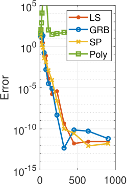
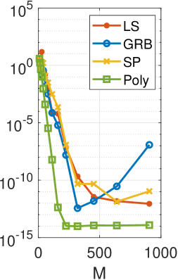
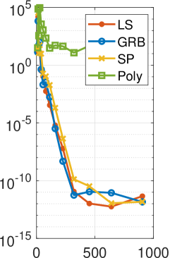
Figure 3: Runge’s example: computed error, square case $M=N^{(\mathcal{L})}$. The left panel is the case of equispaced nodes, the center is the case of Chebychev nodes, and the right is the case of randomly generated nodes. Convergence is tested at different choices of the activation function and increasing the number of interpolating nodes $M$ and compared with one of the polynomial interpolation. In this case, the linear problem (15) is squared.

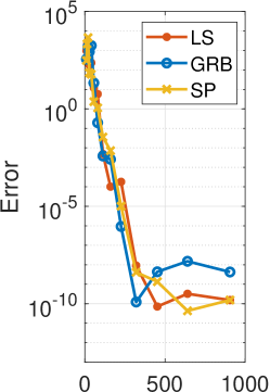
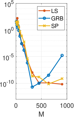
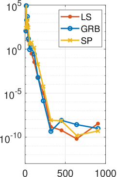
Figure 4: Runge’s example: computed error for the derivative, square case $M=N_{\mathcal{L}}$. The left panel is the case of equispaced nodes, the central panel is the case of Chebychev nodes, and the right panel is the case of randomly generated nodes at different choices of the activation function. The difference is between the exact derivative of a function $f_{R}$ in (16) and the computed derivative of the function obtained by interpolation, the one used in Figure 3.

In figures 3-6 we report the errors obtained when testing our procedure with the target function being Runge’s one and its derivative. In the first two, figures 3-4 the convergence is done in the squared case $M=N^{(\mathcal{L})}$, respectively interpolating the function (16) and its derivative. In the first case, we can notice that the convergence is exponential although not optimal, i.e. geometrical but with a different constant. Surprisingly, exponential convergence is independent of the choice of the interpolation nodes. Convergence in all cases is obtained up to a precision that is related to the condition of the linear problem (15) that is solved. We point out that no particular care has been taken for the resolution of such a problem: all tests are done via the backslash command in MATLAB: recall that the determination of the parameters of the ANN does not involve optimization: the internal parameters are fixed via ELM and the external weights are solved through a square linear problem.

In the second case, the one reported in Figure 4, we plot the errors obtained for the approximation of the derivative of Runge’s function in the squared case. We compute the interpolant as in the first case and then evaluate the error that is done with respect to the derivative of the original functions. This can be done in our case because both the exact derivative of the function $f_{R}$ and the exact derivative of the interpolating ANN can be done in an exact way. From the reported test we can conclude that the convergence of the network function is exponential also in this case, which reveals a surprising ability of such interpolating ANN to approximate very well also the derivative of the function. Polynomial interpolation is not well suited for the approximation of the derivative of an interpolated function so the results of this test are not reported in the figures.

In order to recover the exact optimal convergence for Runge’s example, we consider the overparametrized ANN and fix $M=N^{(\mathcal{L})}/2$. Recall that the interpolation problem (15) for the single-layer ANN (13) remains linear in the unknowns - free parameters - $w$ so that the training is reduced to the resolution of an underdeterminated system, ad ex. via least squares. In Figures 5 and 6 we report the results obtained in this overparametrized case for the function itself and for its derivative, respectively. Error convergence is optimal in this case, see equation (17), and we notice again that is independent of the choice of the interpolation nodes. To emphasize this, we report in a black triangle the reference convergence, interpolating polynomials on Chebychev nodes. The least-square procedure, then, adapts the solution in this overparametrized setting, so that the enrichment of the space is effectively used even if the number of interpolating points does not match the number of independent functions used for approximation. For these reasons, we propose this overparametrization as the procedure for all the next numerical tests.

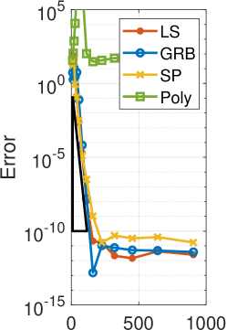
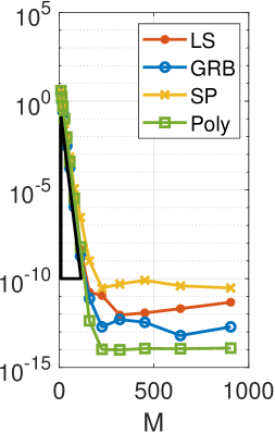
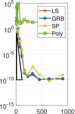
Figure 5: Runge’s example: computed error with respect to the number of interpolating nodes $M$, overparametrized case with $M=N^{(\mathcal{L})}/2$. The left panel is the case of equispaced nodes, the central panel is the case of Chebychev nodes, the right panel is the case of randomly generated nodes. The linear problem (15) is solved by least squares. The black triangle is the reference convergence (interpolating polynomial on Chebychev nodes), as reported in (17).

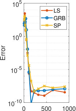
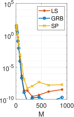
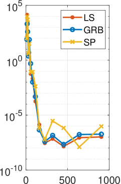
Figure 6: Runge’s example: computed error for the derivative with respect to the number of interpolating nodes $M$, overparametrized case with $M=N^{(\mathcal{L})}/2$. The left panel is the case of equispaced nodes, the central panel is the case of Chebychev nodes, and the right panel is the case of randomly generated nodes. The difference is between the exact derivative of function $f_{R}$ in (16) and the computed derivative of the function obtained by interpolation, the one used in Figure 5.

3.2 Other function approximation tests

In this section, we present some examples to test our procedure with the target function being various regular functions.

Notation follows what was presented in the previous section. The reference interval is always $[-1,1]$. The considered test covers all possible behaviors of regular functions and we consider:

• a polynomial function (Section 3.2.1);

• analytic functions of the three possible types: analytic in the whole complex plane, analytic in the reference domain with a pole far away from the domain, analytic with poles in the complex plane near the considered domain (Section 3.2.2);

• functions with lower regularities (Section 3.2.3).

Moreover, while selecting such functions, we include also highly oscillating and steep gradient behaviors: all examples in sections 3.2.2-3.2.3 follow the work reported in [35].

3.2.1 Polynomial function

In this section, we present a polynomial example to test the accuracy and stability of our procedure. We generate, with a random procedure based on the $randi$ function of Matlab, the following:

$$f(x)=4x^{16}-4x^{15}+8x^{13}+8x^{12}-8x^{11}-6x^{10}-9x^{9}-x^{8}-10x^{7}-x^{6}+3x^{5}-5x^{4}+4x^{3}+2x^{2}-10x+1$$

This test is of particular interest because our choice of network does not reproduce polynomials, thus, as expected, also in this case we can evaluate convergence but not exactness. Then, the aim is to test the accuracy of our procedure and, by considering increasing numbers of degrees of freedom, the stability. In Figure 7 we notice that the convergence is exponential, and stops at different accuracy levels, which is expected due to the difference in condition number when the location of nodes is changed. Also, stability is confirmed, being in all tests the higher accuracy is maintained when the number of nodes increases. As already noticed in Runge’s example, we obtain good accuracy in all tests, and independently of the location of nodes as we present tests done on three different sets of interpolation nodes and the convergence is maintained.

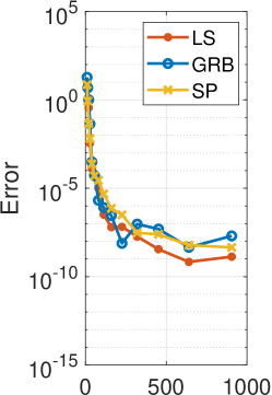
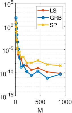
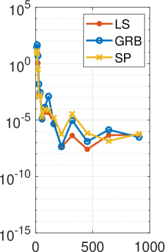
Figure 7: Interpolation of a polynomial function: computed error, overparametrized case with $M=N^{(\mathcal{L})}/2$. Convergence is tested at different choices of the activation function and increasing the number of interpolating nodes $M$. The left panel is the case of equispaced nodes, the central panel is the case of Chebychev nodes, and the right panel is the case of randomly generated nodes. The linear problem (15) is solved by least squares. Convergence is reported in a semi-log scale.

3.2.2 Other analytic functions

In this section, we present some examples to test the accuracy and stability of our procedure when applied to target functions that are analytic functions in the reference interval. In particular, the functions selected are those investigated in [35], in order to have benchmark results on the convergence rate and we compare the convergence of our network function with the geometric convergence of the polynomial interpolation on Chebychev nodes.

The first example that we present is $f(x)=\cos(20x)$ that is analytic not just on $[-1,1]$, but in the whole complex plane, and the convergence expected for the polynomial interpolation on the Chebychev nodes is even faster than geometric. Moreover, this function is rapidly oscillating in $[-1,1]$. In Figure 8 we report the computed error. We observe again that by applying our procedure we obtain convergence independently on the choice of the interpolation nodes. Also, as before, we notice that the convergence stops at different accuracy levels, due to the condition number of location of the interpolation nodes.

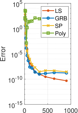
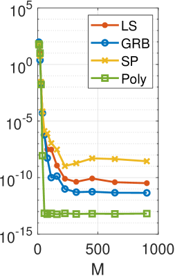
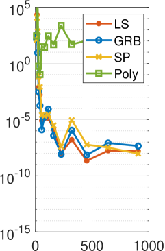
Figure 8: Interpolation of the rapidly oscillating function $cos(20x)$: computed approximation error, overparametrized case with $M=N^{(\mathcal{L})}/2$. Convergence is tested at different choices of the activation function and increasing the number of interpolating nodes $M$ and compared with one of the polynomial interpolation. The expected convergence in the reference case is more than exponential. The left panel is the case of equispaced nodes, the central panel is the case of Chebychev nodes, and the right panel is the case of randomly generated nodes. The linear problem (15) is solved by least squares. Convergence is reported in a semi-log scale.

The second example that we present is for the target function $f(x)=\sqrt{2-x}$, which is an example of a function with a real singularity, that has a branch outside of the considered interval, and relatively far away. We obtain good accuracy in all tests reported in Figure 9. As before, we can notice again that the procedure is stable and that the convergence is independent of the choice of the location of interpolation nodes and also that the convergence stops at different accuracy levels, due to the condition number of location of the interpolation nodes.

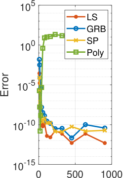
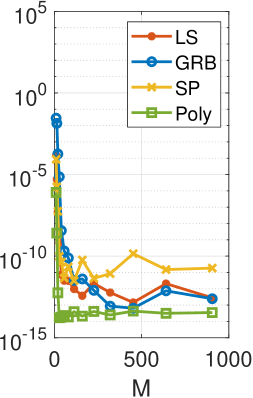
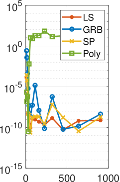
Figure 9: Interpolation of the analytic function with a real singularity $\sqrt{(2-x)}$: computed error with respect to the number of interpolating nodes $M$, overparametrized case with $M=N^{(\mathcal{L})}/2$. The left panel is the case of equispaced nodes, the central panel is the case of Chebychev nodes, and the right panel is the case of randomly generated nodes. The linear problem (15) is solved by least squares. Convergence is reported in a semi-log scale.

As a last example of an analytic function, we test the sharp gradient function $f(x)=tanh(50\pi x)$. This function is a more extreme but entirely analogous example of the Runge function. Indeed it has two poles, but at $\pm 0.01i$, thus closer to the analyzed interval $[-1,1]$. This makes the polynomial interpolation on Chebychev nodes, for the theory explained in [35], much slower, though still robust. Figure 10 shows also in this case that our procedure shows the reference convergence -reported in the black triangle- of the interpolating polynomial on Chebychev nodes, and this convergence rate is independent of the choice of the location of interpolation nodes.

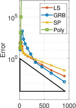
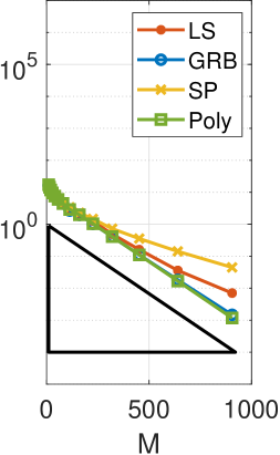
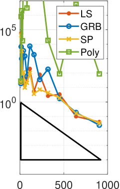
Figure 10: Interpolation of the peaked function $tanh(50\pi x)$: computed error with respect to the number of interpolating nodes $M$, overparametrized case with $M=N^{(\mathcal{L})}/2$. The left panel is the case of equispaced nodes, the central panel is the case of Chebychev nodes, and the right panel is the case of randomly generated nodes. The linear problem (15) is solved by least squares. Convergence is reported in a semi-log scale. The black triangle in the reference convergence (interpolating polynomial on Chebychev nodes).

3.2.3 Differentiable functions

We now present some examples to test the accuracy and stability of our procedure under different regularity hypotheses of the target functions. We use differentiable functions again selected among the functions examined in [35] to study the smoothness-approximability link. More precisely, the analyzed functions are, for an integer $\nu\geq 0$, $\nu-1$ times differentiable and with the $(\nu-1)$–th derivative absolutely continuous and $\nu$–th derivative of bounded variation in $[-1,1]$. From the results of Theorem 7.2 in [35], this implies the convergence at the algebraic rate $O(M^{-\nu})$ of the polynomial interpolation on Chebychev nodes. In these cases, we pass from an exponential to a polynomial convergence rate with respect to the number of nodes.

The first function that we use is $f(x)=\left|{x}\right|$, which is once differentiable with a jump in the first derivative at $x=0$, thus it belongs to the space $C^{0}([-1,1])$. In Figure 11 we plot the computed error in a log-log scale and the convergence curve of our procedure nicely matches $M^{-1}$ in all tests. Thus, not only it matches the theoretic convergence expected on Chebychev nodes, but also we find the same rate on equispaced and random nodes where the polynomial interpolation diverges.

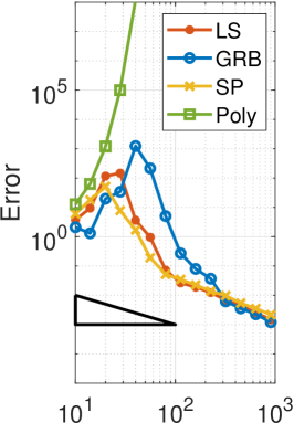
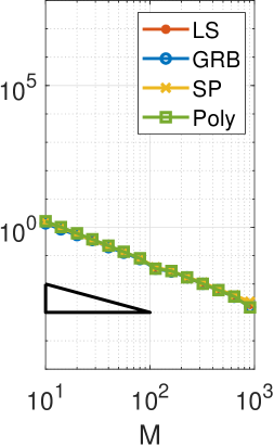
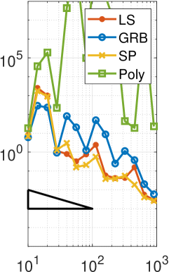
Figure 11: Interpolation of the $C^{0}$ function $\left|{x}\right|$: computed error with respect to the number of interpolating nodes $M$, overparametrized case with $M=N^{(\mathcal{L})}/2$. The left panel is the case of equispaced nodes, the central panel is the case of Chebychev nodes, and the right panel is the case of randomly generated nodes. The linear problem (15) is solved by least squares. Convergence is reported in a log-log scale. The black triangle in the reference convergence (interpolating polynomial on Chebychev nodes).

The second function that we use is $f(x)=\left|\sin 5x\right|^{3}$ which is three times differentiable with jumps in the third derivative at $x=0$ and $x=\pm\pi/5$, thus it belongs to the space $C^{2}([-1,1])$. In Figure 12 we report the errors obtained in a log-log scale and we observe a similarity with what is predicted for the polynomial interpolation on Chebychev nodes, finding that the convergence curve of our procedure nicely matches $M^{-3}$ in all tests. Again, the same accuracy is observed for all the choices of the interpolation nodes.

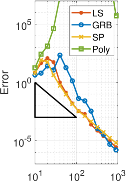
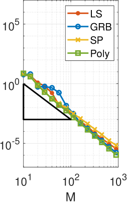
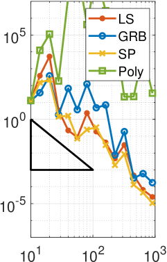
Figure 12: Interpolation of the $C^{2}$ function $\left|\sin{5x}\right|^{3}$: computed error with respect to the number of interpolating nodes $M$, overparametrized case with $M=N^{(\mathcal{L})}/2$. The left panel is the case of equispaced nodes, the central panel is the case of Chebychev nodes, and the right panel is the case of randomly generated nodes. The linear problem (15) is solved by least squares. Convergence is reported in a log-log scale. The black triangle is the reference convergence (interpolating polynomial on Chebychev nodes).

4 Conclusion

In the present paper, we have solved the problem of function approximation via interpolation within a class of single-layer artificial neural networks. Such class of ANN is trained via a procedure, named ELM, that involves a random determination of internal parameters, given that the determination of the free parameters is a linear problem. We conclude that the ANN interpolating function constructed as overparametrized ANN trained via ELM is a very good approximating function: the approximation error converges in most cases with the same rate with respect to the reference method when increasing the number of neurons, while keeping linear the approximation problem to be solved. The first example that is taken into account in the present paper is Runge’s function, where no divergence shows up also taking equispaced or randomly generating nodes. In this and all other test cases, also rapidly oscillating and steep, the function is properly approximated and the approximation error decreases. We suggest that if the target function is regular there is no need for deep structure in the ANN nor the training of internal parameters.

Declarations

Funding This work was partially supported by the Istituto Nazionale di Alta Matematica - Gruppo Nazionale per il Calcolo Scientifico (INdAM-GNCS), Italy.
Open Access funding enabled and organized by Italy Transformative Agreement.
Acknowledgements Francesco Calabrò and Maria Roberta Belardo are members of GNCS-INdAM.
Data availability Data sharing is not applicable to this article as no datasets were generated during the current study.
Conflict of interest The authors declare that they have no conflict of interest.
Open Access This article is licensed under a Creative Commons Attribution 4.0 International License, which permits use, sharing, adaptation, distribution and reproduction in any medium or format, as long as you give appropriate credit to the original author(s) and the source, provide a link to the Creative Commons licence, and indicate if changes were made. The images or other third party material in this article are included in the article’s Creative Commons licence, unless indicated otherwise in a credit line to the material. If material is not included in the article’s Creative Commons licence and your intended use is not permitted by statutory regulation or exceeds the permitted use, you will need to obtain permission directly from the copyright holder. To view a copy of this licence, visit http://creativecommons.org/licenses/by/4.0/ .

References

- [1] Ben Adcock, Rodrigo B Platte, and Alexei Shadrin. Optimal sampling rates for approximating analytic functions from pointwise samples. IMA Journal of Numerical Analysis, 39(3):1360–1390, 05 2018.
- [2] Andrew R Barron. Universal approximation bounds for superpositions of a sigmoidal function. IEEE Transactions on Information theory, 39(3):930–945, 1993.
- [3] Zachary Battles and Lloyd N Trefethen. An extension of matlab to continuous functions and operators. SIAM Journal on Scientific Computing, 25(5):1743–1770, 2004.
- [4] Richard E Bellman. Dynamic programming. Princeton University Press, 1957.
- [5] Christopher M Bishop. Pattern recognition and machine learning. springer, 2006.
- [6] John P Boyd and Jun Rong Ong. Exponentially-convergent strategies for defeating the runge phenomenon for the approximation of non-periodic functions, part i: single-interval schemes. Comput. Phys, 5(2-4):484–497, 2009.
- [7] David Broomhead and David Lowe. Radial basis functions, multi-variable functional interpolation and adaptive networks. Royal Signals and Radar Establishment Malvern (UK), 4148, 03 1988.
- [8] F Calabrò and A Corbo Esposito. An evaluation of clenshaw–curtis quadrature rule for integration wrt singular measures. Journal of computational and applied mathematics, 229(1):120–128, 2009.
- [9] Francesco Calabrò, Gianluca Fabiani, and Constantinos Siettos. Extreme learning machine collocation for the numerical solution of elliptic pdes with sharp gradients. Computer Methods in Applied Mechanics and Engineering, 387:114188, 2021.
- [10] Robert M Corless and Leili Rafiee Sevyeri. The Runge example for interpolation and Wilkinson’s examples for rootfinding. SIAM Review, 62(1):231–243, 2020.
- [11] Eric C Cyr, Mamikon A Gulian, Ravi G Patel, Mauro Perego, and Nathaniel A Trask. Robust training and initialization of deep neural networks: An adaptive basis viewpoint. In Mathematical and Scientific Machine Learning, pages 512–536. PMLR, 2020.
- [12] Tobin A Driscoll, Nicholas Hale, and Lloyd N Trefethen. Chebfun guide. Pafnuty Publications, Oxford, 2014.
- [13] C. E, W. Ma and L. Wu. The Barron space and the flow-induced function spaces for neural network models. Constructive Approximation, 55(1):369–406, 2022.
- [14] W. E, C. Ma, S. Wojtowytsch, and L. Wu. Towards a mathematical understanding of neural network-based machine learning: What we know and what we don’t. arXiv:2009.10713, 2020.
- [15] B. Fornberg, E. Larsson, and N. Flyer. Stable computations with gaussian radial basis functions. SIAM Journal on Scientific Computing, 33(2):869–892, 2011.
- [16] Jiequn Han, Arnulf Jentzen, and E Weinan. Solving high-dimensional partial differential equations using deep learning. Proceedings of the National Academy of Sciences, 115(34):8505–8510, 2018.
- [17] Catherine F Higham and Desmond J Higham. Deep learning: An introduction for applied mathematicians. SIAM Review, 61(4):860–891, 2019.
- [18] Kurt Hornik, Maxwell Stinchcombe, and Halbert White. Universal approximation of an unknown mapping and its derivatives using multilayer feedforward networks. Neural networks, 3(5):551–560, 1990.
- [19] Andrew Hryniowski and Alexander Wong. Deeplabnet: End-to-end learning of deep radial basis networks with fully learnable basis functions. arXiv preprint arXiv:1911.09257, 2019.
- [20] Guang-Bin Huang, Qin-Yu Zhu, and Chee-Kheong Siew. Extreme learning machine: theory and applications. Neurocomputing, 70(1-3):489–501, 2006.
- [21] Ameya D Jagtap, Yeonjong Shin, Kenji Kawaguchi, and George Em Karniadakis. Deep kronecker neural networks: A general framework for neural networks with adaptive activation functions. arXiv preprint arXiv:2105.09513, 2021.
- [22] Kyong Hwan Jin, Michael T McCann, Emmanuel Froustey, and Michael Unser. Deep convolutional neural network for inverse problems in imaging. IEEE Transactions on Image Processing, 26(9):4509–4522, 2017.
- [23] George Em Karniadakis, Ioannis G Kevrekidis, Lu Lu, Paris Perdikaris, Sifan Wang, and Liu Yang. Physics-informed machine learning. Nature Reviews Physics, pages 1–19, 2021.
- [24] A. Kratsios. The universal approximation property: Characterizations, existence, and a canonical topology for deep-learning. Annals of Mathematics and Artificial Intelligence, 89(5-6):435–469, 2021.
- [25] Moshe Leshno, Vladimir Ya Lin, Allan Pinkus, and Shimon Schocken. Multilayer feedforward networks with a nonpolynomial activation function can approximate any function. Neural networks, 6(6):861–867, 1993.
- [26] Lu Lu, Pengzhan Jin, Guofei Pang, Zhongqiang Zhang, and George Em Karniadakis. Learning nonlinear operators via deeponet based on the universal approximation theorem of operators. Nature Machine Intelligence, 3(3):218–229, 2021.
- [27] Siddhartha Mishra and Roberto Molinaro. Estimates on the generalization error of physics-informed neural networks for approximating a class of inverse problems for PDEs. IMA Journal of Numerical Analysis, jun 2021.
- [28] Jooyoung Park and Irwin W Sandberg. Universal approximation using radial-basis-function networks. Neural computation, 3(2):246–257, 1991.
- [29] Allan Pinkus. Approximation theory of the mlp model. Acta Numerica 1999: Volume 8, 8:143–195, 1999.
- [30] Allan Pinkus. Ridge functions, volume 205. Cambridge University Press, 2015.
- [31] Rodrigo B Platte, Lloyd N Trefethen, and Arno BJ Kuijlaars. Impossibility of fast stable approximation of analytic functions from equispaced samples. SIAM review, 53(2):308–318, 2011.
- [32] Jonathan W Siegel and Jinchao Xu. Approximation rates for neural networks with general activation functions. Neural Networks, 128:313–321, 2020.
- [33] Jonathan W Siegel and Jinchao Xu. High-order approximation rates for shallow neural networks with cosine and reluk activation functions. Applied and Computational Harmonic Analysis, 58:1–26, 2022.
- [34] Lloyd N Trefethen. Is gauss quadrature better than clenshaw–curtis? SIAM review, 50(1):67–87, 2008.
- [35] Lloyd N Trefethen. Approximation Theory and Approximation Practice, Extended Edition. SIAM, 2019.
- [36] Rene Vidal, Joan Bruna, Raja Giryes, and Stefano Soatto. Mathematics of deep learning. arXiv preprint arXiv:1712.04741, 2017.