Foundation Model-oriented Robustness: Robust Image Model Evaluation with Pretrained Models

Abstract

Machine learning has demonstrated remarkable performance over finite datasets, yet whether the scores over the fixed benchmarks can sufficiently indicate the model’s performance in the real world is still in discussion. In reality, an ideal robust model will probably behave similarly to the oracle (e.g., the human users), thus a good evaluation protocol is probably to evaluate the models’ behaviors in comparison to the oracle. In this paper, we introduce a new robustness measurement that directly measures the image classification model’s performance compared with a surrogate oracle (i.e., a foundation model). Besides, we design a simple method that can accomplish the evaluation beyond the scope of the benchmarks. Our method extends the image datasets with new samples that are sufficiently perturbed to be distinct from the ones in the original sets, but are still bounded within the same image-label structure the original test image represents, constrained by a foundation model pretrained with a large amount of samples. As a result, our new method will offer us a new way to evaluate the models’ robustness performance, free of limitations of fixed benchmarks or constrained perturbations, although scoped by the power of the oracle. In addition to the evaluation results, we also leverage our generated data to understand the behaviors of the model and our new evaluation strategies.

1 Introduction

Machine learning has achieved remarkable performance over various benchmarks (Zhang et al., 2023a; Lei et al., 2023; Guo et al., 2022). For example, the recent successes of various neural network architectures (He et al., 2016a; Touvron et al., 2021) has shown strong numerical evidence that the prediction accuracy over specific tasks can reach the position of the leaderboard as high as a human (He et al., 2015; Nangia & Bowman, 2019), suggesting different application scenarios of these methods. However, these methods deployed in the real world often underdeliver its promises made through the benchmark datasets (Edwards, 2019; D’Amour et al., 2020), usually due to the fact that these benchmark datasets, typically i.i.d, cannot sufficiently represent the diversity of the samples a model will encounter after being deployed in practice (Recht et al., 2019; Szegedy et al., 2013; Wang et al., 2020c; Zhang et al., 2023b; Wu et al., 2023; Zhang & Kim, 2023).

Fortunately, multiple lines of study have aimed to embrace this challenge, and most of these works are proposing to further diversify the datasets used at the evaluation time. We notice these works mostly fall into two main categories: (1) the works that study the performance over testing datasets generated by predefined perturbation over the original i.i.d datasets, such as adversarial robustness (Szegedy et al., 2013; Goodfellow et al., 2015) or robustness against certain noises (Geirhos et al., 2019; Hendrycks & Dietterich, 2019; Wang et al., 2020b); and (2) the works that study the performance over testing datasets that are collected anew with a procedure/distribution different from the one for training sets,

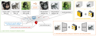
Figure 1: The main structure of our system to generate test images with foundation models and examples of the generated images with their effectiveness in evaluation of model’s robustness.

such as domain adaptation (Ben-David et al., 2007; 2010) and domain generalization (Muandet et al., 2013).

Both of these lines, while pushing the study of robustness evaluation further, mostly have their own advantages and limitations as a tradeoff on how to guarantee the underlying image-label structure of evaluation samples will be the same as the training samples: perturbation based evaluations usually maintain the image-label structure by predefining the perturbations within a set of operations that will not alter the image semantics, such as $\ell$-norm ball constraints (Carlini et al., 2019), or texture (Geirhos et al., 2019), frequency-based (Wang et al., 2020b) perturbations, but are relatively limited in the variety of perturbations allowed. On the other hand, new-dataset based evaluations maintain the image-label structure by soliciting the efforts of human annotators to construct datasets with the same semantics but significantly different styles (Hendrycks et al., 2021b; Hendrycks & Dietterich, 2019; Wang et al., 2019). However, such new datasets may be costly to collect, and a potential issue is that they are fixed once collected and published to the research community. Ranking methods based on the fixed datasets will eventually lead to the selection bias of methods (Duda et al., 1973; Friedman et al., 2001), where the final selection of methods only fits certain datasets rather than being a good reflection of the world. While recent efforts have tried to alleviate the selection bias by collecting data from multiple sources  (Gulrajani & Lopez-Paz, 2020; Koh et al., 2021; Ye et al., 2021), we kindly argue that a dynamic process of generating evaluation datasets will certainly further mitigate this issue.

In this paper, we investigate how to diversify the robustness evaluation datasets to make the evaluation results credible and representative. As shown in Figure 1, we aim to integrate the advantages of the above two directions by introducing a new protocol to generate evaluation datasets that can automatically perturb the samples to be sufficiently different from existing test samples, while maintaining the underlying unknown image-label structure with respect to a foundation model (we use a CLIP (Radford et al., 2021) model in this paper). Based on the new evaluation protocol, we introduce a new robustness metric that measures the robustness compared with the foundation model. Moreover, with our proposed evaluation protocol and metric, we make a study of current robust machine learning techniques to identify the robustness gap between existing models and the foundation model. This is particularly important if the goal of a research direction is to produce models that function reliably to have performance comparable to the foundation model.

Therefore, our contributions in this paper are three-fold:

• We introduce a new robustness metric that measures the robustness gap between models and the foundation model.

• We introduce a new evaluation protocol to generate evaluation datasets that can automatically perturb the samples to be sufficiently different from existing test samples, while maintaining the underlying unknown image-label structure.

• We leverage our evaluation metric and protocol to conduct the very first systematic study on robustness evaluation. We believe that such a study is timely and significant to the community. Our analysis further brings us the understanding and conjectures of the behavior of the deep learning models, opening up future research directions.

2 Background

Current Robustness Evaluation Protocols.

The evaluation of machine learning models in non-i.i.d scenario have been studied for more than a decade, and one of the pioneers is probably domain adaptation (Ben-David et al., 2010). In domain adaptation, the community trains the model over data from one distribution and tests the model with samples from a different distribution; in domain generalization (Muandet et al., 2013), the community trains the model over data from several related distributions and test the model with samples from yet another distribution. A popular benchmark dataset used in domain generalization study is the PACS dataset (Li et al., 2017), which consists of images from seven categories and four domains (photo, art, cartoon, and sketch), and the community studies the empirical performance of models when trained over three of the domains and tested over the remaining one. To facilitate the development of cross-domain robust image classification, the community has introduced several benchmarks, such as PACS (Li et al., 2017), ImageNet-A (Hendrycks et al., 2021b), ImageNet-C (Hendrycks & Dietterich, 2019), ImageNet-Sketch (Wang et al., 2019), and collective benchmarks integrating multiple datasets such as DomainBed (Gulrajani & Lopez-Paz, 2020), WILDS (Koh et al., 2021), and OOD Bench (Ye et al., 2021).

While these datasets clearly maintain the underlying image-label structure of the images, a potential issue is that these evaluation datasets are fixed once collected. Thus, if the community relies on these fixed benchmarks repeatedly to rank methods, eventually the selected best method may not be a true reflection of the world, but a model that can fit certain datasets exceptionally well. This phenomenon has been discussed by several textbooks (Duda et al., 1973; Friedman et al., 2001). While recent efforts in evaluating collections of datasets (Gulrajani & Lopez-Paz, 2020; Koh et al., 2021; Ye et al., 2021) might alleviate the above potential hazards of “model selection with test set”, a dynamic process of generating evaluation datasets will certainly further mitigate this issue.

On the other hand, one can also test the robustness of models by dynamically perturbing the existing datasets. For example, one can test the model’s robustness against rotation (Marcos et al., 2016), texture (Geirhos et al., 2019), frequency-perturbed datasets (Wang et al., 2020b), or adversarial attacks (e.g., $\ell_{p}$-norm constraint perturbations) (Szegedy et al., 2013). While these tests do not require additionally collected samples, these tests typically limit the perturbations to be relatively well-defined (e.g., a texture-perturbed cat image still depicts a cat because the shape of the cat is preserved during the perturbation).

While this perturbation test strategy leads to datasets dynamically generated along the evaluation, it is usually limited by the variations of the perturbations allowed. For example, one may not be able to use some significant distortion of the images in case the object depicted may be deformed and the underlying image-label structure of the images is distorted. Generally speaking, most of the current perturbation-based test protocols are scoped by the tradeoff that a minor perturbation might not introduce enough variations to the existing datasets, while a significant perturbation will potentially destroy the underlying image-label structures.

Assumed Desiderata of Robustness Evaluation Protocol.

As a reflection of the previous discussion, we attempt to offer a summary list of three desired properties of the datasets serving as the benchmarks for robustness evaluation:

• Stableness in Image-label Structure: the most important property of the evaluation datasets is that the samples must represent the same underlying image-label structure as the one in the training samples.

• Effectiveness in Generated Samples: the test samples should be effective in exposing defects for tested models.

• A Dynamic Generation Process: to mitigate selection bias of the models over techniques that focus too attentively to the specification of datasets, ideally, the evaluation protocol should consist of a dynamic set of samples, preferably generated with the tested model in consideration.

Key Contribution: To the best of our knowledge, there are no other evaluation protocols of model robustness that can meet the above three properties simultaneously. Thus, we aim to introduce a method that can evaluate model’s robustness that fulfill the three above desiderata at the same time.

Necessity of New Robustness Measurement in Dynamic Evaluation Protocol.

In previous experiments, we always have two evaluation settings: the “standard” test set, and the perturbed test set. When comparing the robustness of two models, prior arts would be to rank the models by their accuracy under perturbed test set (Geirhos et al., 2019; Hendrycks et al., 2021a; Orhan, 2019; Xie et al., 2020; Zhang, 2019) or other quantities distinct from accuracy, e.g., inception score (Salimans et al., 2016), effective robustness (Taori et al., 2020) and relative robustness (Taori et al., 2020). These metrics are good starting points for experiments since they are precisely defined and easy to apply to evaluate robustness interventions. In the dynamic evaluation protocols, however, these quantities alone cannot provide a comprehensive measure of robustness, as two models are tested on two different “dynamical” test sets. When one model outperforms the other, we cannot distinguish whether one model is actually better than the other, or if the test set happened to be easier.

The core issue in the preceding example is that we can not find the consistent robustness measurement between two different test sets. In reality, an ideal robust model will probably behave similarly to the foundation model (e.g., the human users). Thus, instead of indirectly comparing models’ robustness with each other, a measurement that directly measures models’ robustness compared with the foundation model is desired.

3 Method - Counterfactual Generation with Surrogate Oracle

3.1 Method Overview

We use $(\mathbf{x},\mathbf{y})$ to denote an image sample and its corresponding label, and use $\theta(\mathbf{x})$ to denote the model we aim to evaluate, which takes an input of the image and predicts the label.

  Input: $(\mathbf{X},\mathbf{Y})$, $\theta$, $g$, $h$, total number of iterations $\mathbf{B}$

  Output: generated dataset $(\widehat{\mathbf{X}},\mathbf{Y})$

  for each $(\mathbf{x},\mathbf{y})$ in $(\mathbf{X},\mathbf{Y})$ do

     generate $\widehat{\mathbf{x}}_{0}=g(\mathbf{x},\mathbf{b}_{0})$

     if $h(\widehat{\mathbf{x}}_{0})=\mathbf{y}$ then

        set $\widehat{\mathbf{x}}=\widehat{\mathbf{x}}_{0}$

        for iteration $\mathbf{b}_{t}<\mathbf{B}$ do

           generate $\widehat{\mathbf{x}}_{t}=g(\widehat{\mathbf{x}}_{t-1},\mathbf{b}_{t})$

           if $h(\widehat{\mathbf{x}}_{t})=\mathbf{y}$ then

              set $\widehat{\mathbf{x}}=\widehat{\mathbf{x}}_{t}$

           else

              set $\widehat{\mathbf{x}}=\widehat{\mathbf{x}}_{t-1}$

              exit FOR loop

           end if

        end for

     else

        set $\widehat{\mathbf{x}}=\mathbf{x}$

     end if

     use $(\widehat{\mathbf{x}},\mathbf{y})$ to construct $(\widehat{\mathbf{X}},\mathbf{Y})$

  end for

Algorithm 1 Perturbed Image Generation with Foundation Models

We use $g(\mathbf{x},\mathbf{b})$ to denote an image generation system, which takes an input of the starting image $\mathbf{x}$ to generate the another image $\widehat{\mathbf{x}}$ within the computation budget $\mathbf{b}$. The generation process is performed as an optimization process to maximize a scoring function $\alpha(\widehat{\mathbf{x}},\mathbf{z})$ that evaluates the alignment between the generated image and generation goal $\mathbf{z}$ guiding the perturbation process. The higher the score is, the better the alignment is. Thus, the image generation process is formalized as

$$\widehat{\mathbf{x}}=\operatorname*{arg\,max}_{\widehat{\mathbf{x}}=g(\mathbf{x},\mathbf{b}),\mathbf{b}<\mathbf{B}}\alpha(g(\mathbf{x},\mathbf{b}),\mathbf{z}),$$

where $\mathbf{B}$ denotes the allowed computation budget for one sample. This budget will constrain the generated image not far from the starting image so that the generated one does not converge to a trivial solution that maximizes the scoring function.

In addition, we choose the model classification loss $l(\theta(\widehat{\mathbf{x}}),\mathbf{y})$ as $\mathbf{z}$. Therefore, the scoring function essentially maximizes the loss of a given image in the direction of a different class.

Finally, to maintain the unknown image-label structure of the images, we leverage the power of the pretrained giant models to scope the generation process: the generated images must be considered within the same class by the pretrained model, denoted as $h(\widehat{\mathbf{x}})$, which takes in the input of the image and makes a prediction.

Connecting all the components above, the generation process will aim to optimize the following:

$$\widehat{\mathbf{x}}= \operatorname*{arg\,max}_{\widehat{\mathbf{x}}=g(\mathbf{x},\mathbf{b}),\mathbf{b}<\mathbf{B},\mathbf{z}=l(\theta(\widehat{\mathbf{x}}),\mathbf{y})}\alpha(g(\mathbf{x},\mathbf{b}),\mathbf{z}),$$

$$\textnormal{subject to}\quad h(\widehat{\mathbf{x}})=\mathbf{y}.$$

Our method is generic and agnostic to the choices of the three major components, namely $\theta$, $g$, and $h$. For example, the $g$ component can vary from something as simple as basic transformations adding noises or rotating images to a sophisticated method to transfer the style of the images; on the other hand, the $h$ component can vary from an approach with high reliability and low efficiency such as actually outsourcing the annotation process to human labors to the other polarity of simply assuming a large-scale pretrained model can function plausibly as a human.

In the next part, we will introduce our concrete choices of $g$ and $h$ leading to the later empirical results, which build upon the recent advances of vision research.

3.2 Engineering Specification

We use VQGAN (Esser et al., 2021) as the image generation system $g(\mathbf{x},\mathbf{b})$, and the $g(\mathbf{x},\mathbf{b})$ is boosted by the evaluated model $\theta(\mathbf{x})$ serving as the $\alpha(\widehat{\mathbf{x}},\mathbf{z})$ to guide the generation process, where $\mathbf{z}=l(\theta(\widehat{\mathbf{x}}),\mathbf{y})$ is the model classification loss on current perturbed images.

The generation is an iterative process guided by the scoring function: at each iteration, the system adds more style-wise transformations to the result of the previous iteration. Therefore, the total number of iterations allowed is denoted as the budget $\mathbf{B}$ (see Section 4.5 for details of finding the best perturbation). In practice, the value of budget $\mathbf{B}$ is set based on the resource concerns.

To guarantee the image-label structure of images, we use a CLIP (Radford et al., 2021) model to serve as $h$, and design the text fragment input of CLIP to be “an image of {class}”. We directly optimize VQGAN encoder space which is guided by our scoring function. We show the algorithm in Algorithm 1.

3.2.1 Sparse Submodel of VQGAN for Efficient Perturbation

While our method will function properly as described above, we notice that the generation process still has a potential limitation: the bound-free perturbation of VQGAN will sometimes perturb the semantics of the images, generating results that will be rejected by the foundation model later and thus leading to a waste of computational efforts.

To counter this challenge, we use a sparse variable selection method to analyze the embedding dimensions of VQGAN to identify a subset of dimensions that is mainly responsible for the non-semantic variations.

In particular, with a dataset $(\mathbf{X},\mathbf{Y})$ of $n$ samples, we first use VQGAN to generate a style-transferred dataset $(\mathbf{X}^{\prime},\mathbf{Y})$. During the generation process, we preserve the latent representations of input samples after the VQGAN encoder in the original dataset. We also preserve the final latent representations before the VQGAN decoder that are quantized after the iterations in the style-transferred dataset. Then, we create a new dataset $(\mathbb{E},\mathbf{L})$ of $2n$ samples, for each sample $(\mathbf{e},l)\in(\mathbb{E},\mathbf{L})$, $\mathbf{e}$ is the latent representation for the sample (from either the original dataset or the style-transferred one), and $l$ is labelled as 0 if the sample is from the original dataset and 1 if the style-transferred dataset.

Then, we train $\ell_{1}$ regularized logistic regression model to classify the samples of $(\mathbb{E},\mathbf{L})$. With $\mathbf{w}$ denoting the weights of the model, we solve the following problem

$$\operatorname*{arg\,min}_{\mathbf{w}}\sum_{(\mathbf{e},l)\in(\mathbb{E},\mathbf{L})}l(\mathbf{e}\mathbf{w},l)+\lambda\|\mathbf{w}\|_{1},$$

and the sparse pattern (zeros or not) of $\mathbf{w}$ will inform us about which dimensions are for the style.

3.3 Measuring Robustness

Foundation Model-oriented Robustness (FMR). By design, the image-label structures of perturbed images will be maintained by the foundation model. Thus, if a model has a smaller accuracy drop on the perturbed images, it means that the model makes more similar predictions to foundation model compared to a different model. To precisely define FMR, we introduce perturbed accuracy (PA), the accuracy on the perturbed images that our generative model successfully produces. As the standard accuracy (SA) may influence PA to some extent, to disentangle PA from SA, we normalize PA with SA as FMR:

$$\textnormal{FMR}=\frac{\textnormal{PA}}{\textnormal{SA}}\times 100\%$$

In settings where the foundation model is human labors, FMR measures the robustness difference between the evaluated model and human perception. In our experiment setting, FMR measures the robustness difference between models trained on fixed datasets (the tested model) and the model trained on unfiltered, highly varied, and highly noisy data (the CLIP).

At last, we devote a short paragraph to kindly remind some readers that, despite the alluring idea of designing systems that forgo the usages of underlying image-label structure or foundation model, it has been proved or argued multiple times that it is impossible to create that knowledge with nothing but data, in either context of machine learning (Locatello et al., 2019; Mahajan et al., 2019; Wang et al., 2021) or causality (Bareinboim et al., 2020; Xia et al., 2021),(Pearl, 2009, Sec. 1.4).

4 Experiments - Evaluation and Understanding of Models

4.1 Experiment Setup

We consider four different scenarios, ranging from the basic benchmark MNIST (LeCun et al., 1998), through CIFAR10 (Krizhevsky et al., 2009), 9-class ImageNet (Santurkar et al., 2019), to full-fledged 1000-class ImageNet (Deng et al., 2009). For ImageNet, we resize all images to $224\times 224~{}\textrm{px}$. We also center and re-scale the color values with $\mu_{RGB}=[0.485,0.456,0.406]$ and $\sigma=[0.229,0.224,0.225]$. The perturbation step size for each iteration is 0.001. The total number of iterations allowed (computation budget $\mathbf{B}$) is 50.

For each of the experiment, we report a set of four results:

• Standard Accuracy (SA): reported for references.

• Perturbed Accuracy (PA): accuracy on the images our generation process successfully produces a perturbed image.

• Foundation Model-oriented Robustness (FMR): robustness of the model compared with the foundation model.

4.2 Robustness Evaluation for Standard Vision Models

We consider a large range of models (Appedix M) and evaluate pre-trained variants of a LeNet architecture (LeCun et al., 1998) for the MNIST experiment and ResNet architecture (He et al., 2016a) for the remaining experiments. For ImageNet experiment, we also consider pretrained transformer variants of ViT (Dosovitskiy et al., 2020), Swin (Liu et al., 2021), Twins (Chu et al., 2021), Visformer (Chen et al., 2021) and DeiT (Touvron et al., 2021) from the timm library (Wightman, 2019). We evaluate the recent ConvNeXt (Liu et al., 2022) as well. All models are trained on the ILSVRC2012 subset of IN comprised of 1.2 million images in the training and a total of 1000 classes (Deng et al., 2009; Russakovsky et al., 2015).

Table 1: The robustness test of standard models. We note 1) there exists a performance gap between standard models and the foundation model, and 2) transformer-variants outperform the vanilla ResNet in terms of FMR.

Data	Model	SA	PA	FMR
MNIST	LeNet	99.09	27.78	28.04
CIFAR10	ResNet18	95.38	52.34	54.88
9-class IN	ResNet18	92.30	27.95	30.28
ImageNet	ResNet50	76.26	33.15	43.47
	ViT	82.40	41.65	50.55
	DeiT	78.57	43.25	55.05
	Twins	80.53	48.52	60.25
	Visformer	79.88	47.82	59.87
	Swin	81.67	56.95	69.73
	ConvNeXt	82.05	47.68	58.11

We report our results in Table 1. As expected, these models can barely maintain their performances when tested on data from different distributions, as shown by many previous works (e.g., Geirhos et al., 2019; Hendrycks & Dietterich, 2019; Wang et al., 2020b).

Interestingly, on ImageNet, though both transformer-variants models and vanilla CNN-architecture model, i.e., ResNet, attain similar clean image accuracy, transformer-variants substantially outperform ResNet50 in terms of FMR under our dynamic evaluation protocol. We conjecture such a performance gap partly originated from the differences in training setups; more specifically, it may be resulted by the fact transformer-variants by default use strong data augmentation strategies while ResNet50 use none of them. The augmentation strategies (e.g., Mixup (Zhang et al., 2017), Cutmix (Yun et al., 2019) and Random Erasing (Zhong et al., 2020), etc.) already naively introduce out-of-distribution (OOD) samples during training, therefore are potentially helpful for securing model robustness towards data shifts. When equiping with the similar data augmentation strategies, CNN-architecture model, i.e., ConvNext, has achieved comparable performance in terms of FMR. This hypothesis has also been verified in recent works (Bai et al., 2021; Wang et al., 2022b). We will offer more discussions on the robustness enhancing methods in Section 4.3.

Surprisingly, we notice a large difference within the transformer family in the proposed FMR metric. Despite Swin Transformer’s suboptimal accuracy on the standard dataset, it achieves the best FMR. One possible reason for this phenomenon may due to their internal architecture that are related to the self-attention (SA) mechanism. Therefore, we conduct in-depth analysis on the effects of head numbers. The results reveal that increased head numbers enhance expressivity and robustness, albeit at the expense of clean accuracy. More details can be found in Appendix C.

Besides comparing performance between different standard models, FMR brings us the chance to directly compare models with the foundation model. Across all of our experiments, the FMR shows the significant gap between models and the foundation model, which is trained on the unfiltered and highly varied data, seemingly suggesting that training with a more diverse dataset would help with robustness. This overarching trend has also been identified in (Taori et al., 2020). However, quantifying when and why training with more data helps is still an interesting open question.

4.3 Robustness Evaluation for Robust Vision Models

Recently, some techniques have been introduced to cope with corruptions or style shifts. For example, by adapting the batch normalization statistics with a limited number of samples (Schneider et al., 2020), the performance on stylized images (or corrupted images) can be significantly increased. Additionally, some more sophisticated techniques, e.g., DAT (Mao et al., 2022b), have also been widely employed by the community.

To investigate whether those OOD robust models can still maintain the performance in our dynamic evaluation, we evaluate the pretrained ResNet50 models combining with the five leading methods from the ImageNet-C leaderboard, namely Stylized ImageNet training (SIN; (Geirhos et al., 2019)), adversarial noise training (ANT; (Rusak et al., )) as well as a combination of ANT and SIN (ANT+SIN; (Rusak et al., )), optimized data augmentation using Augmix (AugMix; (Hendrycks et al., 2019)), DeepAugment (DeepAug; (Hendrycks et al., 2021a)), a combination of Augmix and DeepAugment (DeepAug+AM; (Hendrycks et al., 2021a)) and Discrete Adversarial Training (DAT; (Mao et al., 2022b)).

Table 2: The robustness test of generated countefactual images for OOD robust models. $\rm SA^{*}$ represents the model’s top-1 accuracy on ImageNet-C dataset. We note applying DeepAug+AM yields the best FMR under our dynamic evaluation protocol.

Model	SA	$\rm\mathbf{SA^{*}}$	PA	FMR
ResNet50	76.26	39.20	33.15	43.47
ANT	76.26	50.41	32.73	42.92
SIN	76.24	45.19	32.71	42.90
ANT+SIN	76.26	52.60	33.19	43.52
DeepAug	76.26	52.60	35.33	46.33
Augmix	76.73	48.31	40.94	53.36
DeepAug+AM	76.68	58.10	44.62	58.19
DAT	76.57	68.00	54.63	71.35

The results are displayed in Table 2. Surprisingly, we find that some common corruption robust models, i.e., SIN, ANT, ANT+SIN, fail to maintain their power under our dynamic evaluation protocol. We take the SIN method as an example. The FMR of SIN method is 42.90, which is even lower than that of a vanilla ResNet50. These methods are well fitted in the benchmark ImageNet-C, verifying the weakness of relying on fixed benchmarks to rank methods. The selected best method may not be a true reflection of the real world, but a model well fits certain datasets, which in turn proves the necessity of our dynamic evaluation protocol.

DeepAug, Augmix, DeepAug+AM perform better than SIN and ANT methods in terms of FMR as they dynamically perturb the datasets, alleviating the hazards of “model selection with test set” to some extent. DAT outperform others in terms of FMR, which validates the effectiveness of perturbation in the meaningful symbolic space rather than the continuous pixel space. However, their performance is limited by the variations of the perturbations allowed, resulting in marginal improvements compared with the ResNet50 under our evaluation protocol.

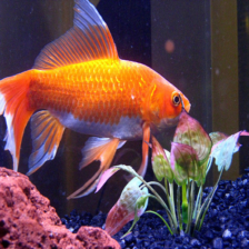
(a) gold fish

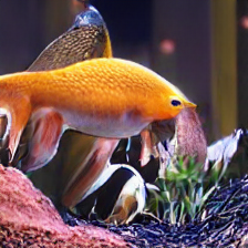
(b) snoek

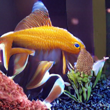
(c) anemone

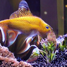
(d) snoek

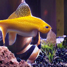
(e) coral reef

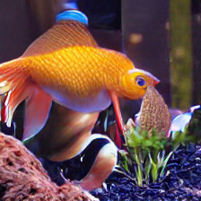
(f) hen

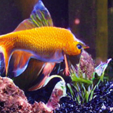
(g) snoek

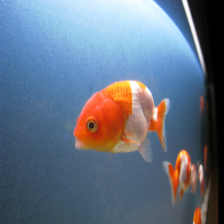
(h) gold fish

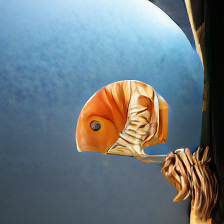
(i) nautilus

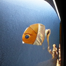
(j) lampshade

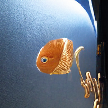
(k) nautilus

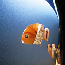
(l) lampshade

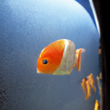
(m) anemone

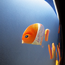
(n) parachute

Figure 2: Visualization of the images generated by our system in evaluating the common corruption robust model, with the original image shown (left image of each row). The caption for each image is either the original label or the predicted label by the corresponding model. The evaluated models are SIN, ANT, ANT+SIN, Augmix, DeepAug and DeepAug+AM from left to right.

Besides, we visualize the perturbed images generated according to the evaluated style-shift robust models in Figure 2. More results are shown in Appendix O. We have the following observations:

Preservation of Local Textual Details. A number of recent empirical findings point to an important role of object textures for CNN, where object textures are more important than global object shapes for CNN model to learn  (Gatys et al., 2015; Ballester & Araujo, 2016; Gatys et al., 2017; Brendel & Bethge, 2019; Geirhos et al., 2019; Wang et al., 2020b). We notice our generated perturbed images may preserve false local textual details, the evaluation task will become much harder since textures are no longer predictive, but instead a nuisance factor (as desired). For the perturbed image generated for the DeepAug method (Figure 2(f)), we produce a skin texture similar to chicken skin, and the fish head becomes more and more chicken-like. ResNet with DeepAug method is misled by this corruption.

Generalization to Shape Perturbations. Moreover, since our attack intensity could be dynamically altered based on the model’s gradient while still maintaining the image-label structures, the perturbation we produce would be sufficient that not just limited to object textures, but even a certain degree of shape perturbation. As it is acknowledged that networks with a higher shape bias are inherently more robust to many different image distortions and reach higher performance on classification and classification tasks, we observe that the perturbed image generated for SIN (Figure 2(b) and Figure 2(i)) and ANT+SIN (Figure 2(d) and Figure 2(k)) methods are shape-perturbed and successfully attack the models.

Recognition of Model Properties. With the combination of different methods, the perturbed images generated would be more comprehensive. For example, the perturbed image generated for DeepAug+AM (Figure 2(g)) would preserve the chicken-like head of DeepAug’s and skin patterns of Augmix’s. As our evaluation method does not memorize the model it evaluated, this result reveals that our method could recognize the model properties, and automatically generate those hard perturbed images to complete the evaluation.

Overall, these visualizations reveal that our evaluation protocol dynamically adjusts attack strategies based on different model properties, and automatically generates effective perturbed images that complement static benchmark, i.e., ImageNet-C, to expose weaknesses for models.

Table 3: Study of different image generator choices on ImageNet dataset. The numbers of PA and FMR are reported. The results of our dynamic evaluation protocol is consistent under different image generator configurations.

Model	ADM		Improved DDPM		Efficient-VDVAE		StyleGAN-XL		VQGAN
	PA	FMR	PA	FMR	PA	FMR	PA	FMR	PA	FMR
ResNet50	33.43	43.84	32.51	42.63	31.37	41.14	32.74	42.93	33.15	43.47
ANT	32.95	43.21	33.62	44.08	32.33	42.39	33.01	43.29	32.73	42.92
SIN	33.23	43.58	33.11	43.43	32.26	42.32	32.46	42.58	32.71	42.90
ANT+SIN	33.49	43.92	34.52	45.26	33.71	44.20	33.99	44.57	33.19	43.52
DeepAug	34.35	45.04	35.44	46.47	34.89	45.75	35.51	46.57	35.33	46.33
Augmix	40.49	52.77	41.20	53.69	40.99	53.42	40.34	52.57	40.94	53.36
DeepAug+AM	44.46	57.98	44.21	57.65	42.35	55.23	42.66	55.64	44.62	58.19

4.4 Understanding the Properties of Our Evaluation System

We continue to investigate several properties of the models in the next couple sections. To save space, we will mainly present the results on CIFAR10 experiment here and save the details to the appendix:

• In Appendix D, we explore the transferability of the generated images. The results of a reasonable transferability suggest that our method of generating images can be potentially used in a broader scope: we can leverage the method to generate a static set of images and set a benchmark to help the development of robustness methods.

• In Appendix E, we test whether initiating the perturbation process with adversarial examples will degrade the FMR. We find that initiaing with FGSM adversarial examples (Goodfellow et al., 2015) barely affect FMR.

• In Appendix F, we compare the vanilla model to a model trained by PGD (Madry et al., 2017). We find that these two models process the data differently. However, their robustness weaknesses are exposed to a similar degree by our test system.

• In Appendix G, we explore the possibility of improving the evaluated robustness by augmenting the images with those generated by our evaluation system. Due to the required computational load, we only use a static set of generated images to train the model and the results suggest that static set of images for augmentation cannot sufficiently robustify the model to our evaluation system.

• We also notice that the generated images tend to shift the color of the original images, so we tested the robustness of grayscale models in Appendix H, the results suggest removing the color channel will not improve robustness performances.

4.5 Experiments Regarding Method Configuration

Generator Configuration. We conduct ablation study on the generator choice to agree on the performance ranking in Table 1 and Table 2. We consider several image generator architechitures, namely, variational autoencoder (VAE) (Kingma & Welling, 2013; Rezende et al., 2014) like Efficient-VDVAE (Hazami et al., 2022), diffusion models (Sohl-Dickstein et al., 2015) like Improved DDPM (Nichol & Dhariwal, 2021) and ADM (Dhariwal & Nichol, 2021), and GAN like StyleGAN-XL (Sauer et al., 2022). As shown in Table 3, we find that the conclusion is consistent under different generator choices, which validates the correctness of our conclusions in Section 4.2 and Section 4.3.

Sparse VQGAN. For scenarios with limited computing resources, we consider sprsifying the VQGAN to speedup the generation process. In experiments of sparse VQGAN, we find that only 0.69% dimensions are highly correlated to the style. Therefore, we mask the rest 99.31% dimensions to create a sparse submodel of VQGAN for efficient perturbation. The running time can be reduced by 12.7% on 9-class ImageNet and 28.5% on ImageNet, respectively. Details can be found in Appendix I. Therefore, our evaluation protocol is also feasible with limited computing resources.

Step Size. The optimal step size value depends on the computation budget $\mathbf{B}$. With limited computation budget, a larger step size value is required. However, large step size may expose foundation model’s potential limitations and affect the evaluation results (see Appendix J). As shown in Appendix J, with sufficient $\mathbf{B}$, a smaller step size can help mitigate such limitations to some extent and is enough for the application in reality.

5 Discussion

5.1 Discussion on the Bias Issues

Selection Bias. In previous sections, we have mentioned that ranking models based on the fixed datasets will potentially lead to the selection bias of methods (Duda et al., 1973; Friedman et al., 2001). While our dynamic evaluation protocol help mitigates this issue, it is inevitable to introduce other biases when we select specific generators and foundation models. Here, we provide more analyses and discussions.

Bias towards Generators. As our evaluation protocol requires an image generator, the quality or diversity of the generated images may be bounded by the choice of generator. However, Table 3 shows the consistent conclusions made in the paper, which verifies that the proposed method is robust to the choice of generator.

Bias towards the Foundation Models. In Appendix J, we explore the category unbalance issue of the CLIP. We find that CLIP has been influenced by the imbalance sample distributions across the Internet, resulting in perturbed images with varying degrees of difficulty. Fortunately, our configurations can alleviate this problem to a large extent, which is enough for the real applications.

Bias of the Metric. As the generated samples are biased to the CLIP zero-shot performance, "PA" and "FMR" scores will also be biased. In Appendix A, we conduct a theoretical analysis to guarantee the correctness of the proposed method. The results show that both conventional fixed dataset estimator and CLIP can recover the groundtruth distributions, but CLIP can do that with a lower variance. With these theoretical evidence, we kindly argue that bias towards the CLIP is better than bias towards the conventional fixed datasets.

Potential Negative Impacts. Although the bias incurred by CLIP is less detrimental than the biases arisen from fixed benchmark datasets, a more detailed discussion on the potential negative impacts is necessary. Therefore, we discuss the potential negative impacts as well as the societal bias of relying on large models in Appendix K.

5.2 Discussion on the Effects of CLIP’s Zero-shot Performance

Domain Gap Concerns. Although CLIP has impressive zero-shot performance, it may still fail in some specialized application scenarios, e.g., medical images, where the common knowledge from CLIP does not suffice. Ensembling multiple pre-trained models as the foundation model can be a better choice, as CLIP is just one example of our contributions, it can be replaced or adjusted to suit different applications.

Zero-shot Adversarial Robustness Concerns. It is known that CLIP can suffer from adversarial attacks (Mao et al., 2022a). Considering that if someone can have access to the CLIP model weights and perform the attack, the power of the evaluation will degrade. In Appendix L, we explore the zero-shot adversarial robustness of CLIP. We find that the vanilla CLIP shows a better robustness performance through FGSM attack compared with XCiT-L12 (Debenedetti et al., 2022) from the RobustBench Leaderboard (Croce et al., 2020). However, if we continue the attack process, we will eventually obtain the adversary that changes the CLIP’s classification decision to the targeted class.

Fortunately, in production, one can use simple techniques such as gradient masking to protect CLIP’s weights from malicious users, thus, the opportunities of being attacked from a white-box manner are quite low. In terms of black-box attacks, CLIP actually shows a strong resilience, for which we have some supporting evidence in Appendix E (See Appendix L for detailed discussions). Thus, CLIP, especially when equipped with techniques to protect its weights and gradients, might be the closest one to serve as the ideal foundation model to maintain the image-label structure at this moment.

6 Conclusion

In this paper, we first summarized the common practices of model evaluation strategies for robust vision machine learning. We then discussed three desiderata of the robustness evaluation protocol. Further, we offered a simple method that can fulfill these three desiderata at the same time, serving the purpose of evaluating vision models’ robustness across generic i.i.d benchmarks, without requirement on the prior knowledge of the underlying image-label structure depicted by the images, although relying on a foundation model.

Appendix A Distribution Estimation

A.1 Problem Formulation

Given an unknown ground truth distribution:

$$\mathbf{P}=\textnormal{Unknown}(\mu,\Sigma)$$ (1)

where $\mu\in\mathbb{R}^{p}$ and $\Sigma\in\mathbb{R}^{p\times p}$.

All the samples in our study are sampled from this distribution.

We use $\mathbf{X}_{k}$ to denote the $k$^th dataset, with $n_{k}$ samples, and we use $\mathbf{x}_{k,i}$ to denote the $i$^th sample in it.

We aim to consider the estimation of $\mu$ from two different models. The conventional smaller model which operates on only one dataset, and WLOG, we assume the smaller model works on $\mathbf{X}_{0}$; and the bigger, CLIP-style model, which operates on a collection of datasets, we say it works on $m$ datasets, i.e., $\{\mathbf{X}_{1},\mathbf{X}_{2},\mathbf{X}_{3},\dots,\mathbf{X}_{m}\}$, we will compare $\mathbb{E}[\widehat{\mu_{0}}-\mu]$ and $\mathbb{E}[\widehat{\mu_{\textnormal{CLIP}}}-\mu]$, $\textnormal{VAR}(\widehat{\mu_{0}})$ and $\textnormal{VAR}(\widehat{\mu_{\textnormal{CLIP}}})$, $\mathbb{E}[\widehat{\Sigma_{0}}-\Sigma]$ and $\mathbb{E}[\widehat{\Sigma_{\textnormal{CLIP}}}-\Sigma]$ and $\textnormal{VAR}(\widehat{\Sigma_{0}})$ and $\textnormal{VAR}(\widehat{\Sigma_{\textnormal{CLIP}}})$.

Assumption I

Due to dataset collection bias, we assume that, while all the data are sampled with the fixed distribution above, the bias of dataset collection will introduce a bias in the estimation of the true parameter $\mu$, therefore

$$\widehat{\mu_{i}}=\mu+\epsilon_{i}$$ (2)

where

$$\widehat{\mu_{i}}:=\dfrac{1}{n_{i}}\sum^{n_{i}}_{j}\mathbf{x}_{i,j}$$ (3)

and

$$\epsilon_{i}\sim N(\mathbf{0},\mathbf{I})$$ (4)

Assumption II

Due to dataset collection bias, we assume that, while all the data are sampled with the fixed distribution above, the bias of dataset collection will introduce a bias in the estimation of the true parameter $\Sigma$, therefore

$$\widehat{\Sigma_{i}}=\epsilon^{{}^{\prime}}_{i}\Sigma$$ (5)

where

$$\widehat{\Sigma_{i}}:=\dfrac{1}{n_{i}}\sum^{n_{i}}_{j}[(\mathbf{x}_{i,j}-\widehat{\mu_{i}})^{T}(\mathbf{x}_{i,j}-\widehat{\mu_{i}})]$$ (6)

and

$$\epsilon^{{}^{\prime}}_{i}\sim\textnormal{Exp}(\mathbf{1}),$$ (7)

Proposition A.1.

Under Assumptions I and II, we have estimators

$$\mathbb{E}[\widehat{\mu_{\textnormal{CLIP}}}-\mu]=\mathbb{E}[\widehat{\mu_{0}}-\mu], \mathbb{E}[\widehat{\Sigma_{\textnormal{CLIP}}}-\Sigma]=\mathbb{E}[\widehat{\Sigma_{0}}-\Sigma]$$

$$\textnormal{VAR}(\widehat{\mu_{\textnormal{CLIP}}})\leq\textnormal{VAR}(\widehat{\mu_{0}}), \textnormal{VAR}(\widehat{\Sigma_{\textnormal{CLIP}}})\leq\textnormal{VAR}(\widehat{\Sigma_{0}})$$

where $\leq$ holds element-wise.

Proof.

Estimation of $\mu$. Under Assumptions I and II, we have

$$\widehat{\mu_{0}}=\mu+\epsilon_{0}$$ (8)

We can obtain $\mathbb{E}[\widehat{\mu_{0}}-\mu]$ and $\textnormal{VAR}(\widehat{\mu_{0}})$ by marginalizing out the randomness introduced by $\epsilon$:

$$\mathbb{E}[\widehat{\mu_{0}}-\mu]=\mathbb{E}[\mu+\epsilon_{0}-\mu]=\mathbb{E}[\epsilon_{0}]=\mathbf{0}.$$ (9)

$$\textnormal{VAR}(\widehat{\mu_{0}}) =\mathbb{E}[\widehat{\mu_{0}}^{2}]-\mathbb{E}^{2}[\widehat{\mu_{0}}]$$

$$=\mathbb{E}[(\mu+\epsilon_{0})^{2}]-\mathbb{E}^{2}[(\mu+\epsilon_{0})]$$

$$=\mathbb{E}[\mu^{2}+2\mu\epsilon_{0}+\epsilon_{0}^{2}]-(\mu+\mathbb{E}[\epsilon_{0}])^{2}$$

$$=\mathbb{E}[\epsilon_{0}^{2}]-\mathbb{E}^{2}[\epsilon_{0}]$$

$$=\textnormal{VAR}(\epsilon_{0})$$

$$=\mathbf{I}$$ (10)

For $\mathbb{E}[\widehat{\mu_{\textnormal{CLIP}}}-\mu]$ and $\textnormal{VAR}(\widehat{\mu_{\textnormal{CLIP}}})$, we have:

$$\mathbb{E}[\widehat{\mu_{\textnormal{CLIP}}}-\mu]=\mathbb{E}[\dfrac{\sum_{i}^{m}\epsilon_{i}n_{i}}{\sum_{i}^{m}n_{i}}]=\dfrac{\sum_{i}^{m}\mathbb{E}[\epsilon_{i}]n_{i}}{\sum_{i}^{m}n_{i}}=\mathbf{0}.$$ (11)

and

$$\textnormal{VAR}(\widehat{\mu_{\textnormal{CLIP}}}) =\mathbb{E}[\widehat{\mu_{\textnormal{CLIP}}}^{2}]-\mathbb{E}^{2}[\widehat{\mu_{\textnormal{CLIP}}}]$$

$$=\mathbb{E}[(\mu+\epsilon_{\textnormal{CLIP}})^{2}]-\mathbb{E}^{2}[(\mu+\epsilon_{\textnormal{CLIP}})]$$

$$=\mathbb{E}[\mu^{2}+2\mu\epsilon_{\textnormal{CLIP}}+\epsilon_{\textnormal{CLIP}}^{2}]-(\mu+\mathbb{E}[\epsilon_{\textnormal{CLIP}}])^{2}$$

$$=\mathbb{E}[\epsilon_{\textnormal{CLIP}}^{2}]-\mathbb{E}^{2}[\epsilon_{\textnormal{CLIP}}]$$ (12)

Since $\mathbb{E}[\epsilon_{\textnormal{CLIP}}]=\mathbb{E}[\widehat{\mu_{\textnormal{CLIP}}}-\mu]=0$, we have:

$$\textnormal{VAR}(\widehat{\mu_{\textnormal{CLIP}}})=\mathbb{E}[\epsilon_{\textnormal{CLIP}}^{2}]=\mathbb{E}[(\dfrac{\sum_{i}^{m}\epsilon_{i}n_{i}}{\sum_{i}^{m}n_{i}})^{2}]$$ (13)

When we expand the square of sum, we will get the many squared terms (which are left finally) and many more that involves at least one $\mathbb{E}[\epsilon_{i}]\mathbf{z}$, where $\mathbf{z}$ can be any arbitrary stuff, and then since $\mathbb{E}[\epsilon_{i}]=\mathbf{0}$, $\mathbf{z}$ won’t matter. Therefore, we have:

$$\textnormal{VAR}(\widehat{\mu_{\textnormal{CLIP}}})=\mathbb{E}[(\dfrac{\sum_{i}^{m}\epsilon_{i}n_{i}}{\sum_{i}^{m}n_{i}})^{2}]=\dfrac{\sum_{i}^{m}n_{i}^{2}\mathbb{E}[\epsilon_{i}^{2}]}{(\sum_{i}^{m}n_{i})^{2}}$$ (14)

Since $n_{i}\geq 1$ for $i=1,2,...,m$, we have $\sum_{i}^{m}n_{i}^{2}\leq(\sum_{i}^{m}n_{i})^{2}$.

Therefore,

$$\textnormal{VAR}(\widehat{\mu_{\textnormal{CLIP}}})=\dfrac{\sum_{i}^{m}n_{i}^{2}\mathbb{E}[\epsilon_{i}^{2}]}{(\sum_{i}^{m}n_{i})^{2}}\leq\dfrac{(\sum_{i}^{m}n_{i})^{2}\mathbb{E}[\epsilon_{i}^{2}]}{(\sum_{i}^{m}n_{i})^{2}}=\mathbb{E}[\epsilon_{i}^{2}]=\mathbf{I}$$ (15)

Estimation of $\Sigma$. We can obtain $\mathbb{E}[\widehat{\Sigma_{0}}-\Sigma]$ and $\textnormal{VAR}(\widehat{\Sigma_{0}})$ by marginalizing out the randomness introduced by $\epsilon^{{}^{\prime}}$:

$$\mathbb{E}[\widehat{\Sigma_{0}}-\Sigma]=\mathbb{E}[\epsilon^{{}^{\prime}}_{0}\Sigma-\Sigma]=\mathbb{E}[(\epsilon^{{}^{\prime}}_{0}-1)\Sigma]=\mathbb{E}[\epsilon^{{}^{\prime}}_{0}-1]\mathbb{E}[\Sigma]=\mathbf{0}.$$ (16)

$$\textnormal{VAR}(\widehat{\Sigma_{0}}) =\mathbb{E}[\widehat{\Sigma_{0}}^{2}]-\mathbb{E}^{2}[\widehat{\Sigma_{0}}]$$

$$=\mathbb{E}[(\epsilon^{{}^{\prime}}_{0}\Sigma)^{2}]-\mathbb{E}^{2}[\epsilon^{{}^{\prime}}_{0}\Sigma]$$

$$=\mathbb{E}[\epsilon^{{}^{\prime}2}_{0}\Sigma^{2}]-\mathbb{E}^{2}[\epsilon^{{}^{\prime}}_{0}]\mathbb{E}^{2}[\Sigma]$$

$$=\mathbb{E}[\epsilon^{{}^{\prime}2}_{0}]\mathbb{E}[\Sigma^{2}]-\mathbb{E}^{2}[\epsilon^{{}^{\prime}}_{0}]\mathbb{E}^{2}[\Sigma]$$

$$=2\mathbb{E}[\Sigma^{2}]-\mathbb{E}^{2}[\Sigma]$$

$$=2\Sigma^{2}-\Sigma^{2}$$

$$=\Sigma^{2}$$ (17)

For $\mathbb{E}[\widehat{\Sigma_{\textnormal{CLIP}}}-\Sigma]$ and $\textnormal{VAR}(\widehat{\Sigma_{\textnormal{CLIP}}})$, we have:

$$\mathbb{E}[\widehat{\Sigma_{\textnormal{CLIP}}}-\Sigma]=\mathbb{E}[\epsilon^{{}^{\prime}}_{\textnormal{CLIP}}\Sigma-\Sigma]=\mathbb{E}[(\epsilon^{{}^{\prime}}_{\textnormal{CLIP}}-1)\Sigma]=\mathbb{E}[\epsilon^{{}^{\prime}}_{\textnormal{CLIP}}-1]\mathbb{E}[\Sigma]=\mathbf{0}.$$ (18)

$$\textnormal{VAR}(\widehat{\Sigma_{\textnormal{CLIP}}}) =\mathbb{E}[\widehat{\Sigma_{\textnormal{CLIP}}}^{2}]-\mathbb{E}^{2}[\widehat{\Sigma_{\textnormal{CLIP}}}]$$

$$=\mathbb{E}[(\epsilon^{{}^{\prime}}_{\textnormal{CLIP}}\Sigma)^{2}]-\mathbb{E}^{2}[\epsilon^{{}^{\prime}}_{\textnormal{CLIP}}\Sigma]$$

$$=\mathbb{E}[\epsilon^{{}^{\prime}2}_{\textnormal{CLIP}}\Sigma^{2}]-\mathbb{E}^{2}[\epsilon^{{}^{\prime}}_{\textnormal{CLIP}}]\mathbb{E}^{2}[\Sigma]$$

$$=\mathbb{E}[\epsilon^{{}^{\prime}2}_{\textnormal{CLIP}}]\mathbb{E}[\Sigma^{2}]-\mathbb{E}^{2}[\Sigma]$$ (19)

Consider that

$$\widehat{\Sigma_{\textnormal{CLIP}}}=\dfrac{\Sigma^{m}_{i}\Sigma^{n_{i}}_{j}(\mathbf{x}_{i,j}-\widehat{\mu_{\textnormal{CLIP}}})^{2}}{\Sigma^{m}_{i}n_{i}}=\dfrac{\Sigma^{m}_{i}\epsilon^{2}_{\textnormal{CLIP}}n_{i}}{\Sigma^{m}_{i}n_{i}}=\epsilon^{{}^{\prime}}_{\textnormal{CLIP}}\Sigma$$ (20)

We will have:

$$\epsilon^{{}^{\prime}}_{\textnormal{CLIP}}=\dfrac{\epsilon^{2}_{\textnormal{CLIP}}}{\Sigma}$$ (21)

Thus, we have $\epsilon^{{}^{\prime}2}_{\textnormal{CLIP}}=\dfrac{\epsilon^{4}_{\textnormal{CLIP}}}{\Sigma^{2}}$. Next, we will compute $\mathbb{E}[\epsilon^{{}^{\prime}2}_{\textnormal{CLIP}}]$ as follows:

$$\mathbb{E}[\epsilon^{{}^{\prime}2}_{\textnormal{CLIP}}] =\mathbb{E}[\dfrac{\epsilon^{4}_{\textnormal{CLIP}}}{\Sigma^{2}}]$$

$$=\dfrac{\mathbb{E}[\epsilon^{4}_{\textnormal{CLIP}}]}{\Sigma^{2}}$$ (22)

By definition, we have:

$$\epsilon_{\textnormal{CLIP}}=\dfrac{\Sigma^{m}_{i}\Sigma^{n_{i}}_{j}(\mathbf{x}_{i,j}-\widehat{\mu_{i}})}{\Sigma^{m}_{i}n_{i}}$$ (23)

Therefore,

$$\epsilon^{2}_{\textnormal{CLIP}}=\dfrac{(\Sigma^{m}_{i}\Sigma^{n_{i}}_{j}(\mathbf{x}_{i,j}-\widehat{\mu_{i}}))^{2}}{(\Sigma^{m}_{i}n_{i})^{2}}$$ (24)

As the value of $x_{i,j}-\widehat{\mu_{i}}$ can be either positive or negative, we have:

$$\epsilon^{2}_{\textnormal{CLIP}}\leq\dfrac{\Sigma^{m}_{i}\Sigma^{n_{i}}_{j}(\mathbf{x}_{i,j}-\widehat{\mu_{i}})^{2}}{\Sigma^{m}_{i}n_{i}}\dfrac{1}{\Sigma^{m}_{i}{n_{i}}}$$ (25)

Since both $(x_{i,j}-\widehat{\mu_{i}})^{2}$ and $n_{i}$ are positive values, we further have:

$$\epsilon^{2}_{\textnormal{CLIP}}\leq\Sigma^{m}_{i}\dfrac{\Sigma^{n_{i}}_{j}(\mathbf{x}_{i,j}-\widehat{\mu_{i}})^{2})}{n_{i}}\dfrac{1}{\Sigma^{m}_{i}{n_{i}}}=\dfrac{\Sigma^{m}_{i}\widehat{\Sigma_{i}}}{\Sigma^{m}_{i}{n_{i}}}=\dfrac{\Sigma^{m}_{i}\epsilon^{{}^{\prime}}_{i}\Sigma}{\Sigma^{m}_{i}{n_{i}}}$$ (26)

Thus, we can obtain

$$\epsilon^{4}_{\textnormal{CLIP}}\leq\dfrac{(\Sigma^{m}_{i}\epsilon^{{}^{\prime}}_{i}\Sigma)^{2}}{(\Sigma^{m}_{i}{n_{i}})^{2}}=\dfrac{(\Sigma^{m}_{i}\epsilon^{{}^{\prime}}_{i})^{2}\Sigma^{2}}{(\Sigma^{m}_{i}{n_{i}})^{2}}$$ (27)

Therefore, we have:

$$\mathbb{E}[\epsilon^{4}_{\textnormal{CLIP}}]\leq\mathbb{E}[\dfrac{(\Sigma^{m}_{i}\epsilon^{{}^{\prime}}_{i})^{2}\Sigma^{2}}{(\Sigma^{m}_{i}{n_{i}})^{2}}]=\dfrac{\mathbb{E}[(\Sigma^{m}_{i}\epsilon^{{}^{\prime}}_{i})^{2}]\Sigma^{2}}{(\Sigma^{m}_{i}{n_{i}})^{2}}$$ (28)

By Assumption A.1, $\epsilon^{{}^{\prime}}_{i}\sim\textnormal{Exp}(\mathbf{1})$, we have $\mathbb{E}[\epsilon^{{}^{\prime}}_{i}]=1$ and $\textnormal{VAR}(\epsilon^{{}^{\prime}}_{i})=1$.

Since $\epsilon^{{}^{\prime}}_{i}$ are independent with each other, we have:

$$\mathbb{E}[(\Sigma^{m}_{i}\epsilon^{{}^{\prime}}_{i})^{2}] =\textnormal{VAR}(\Sigma^{m}_{i}\epsilon^{{}^{\prime}}_{i})+\mathbb{E}^{2}[\Sigma^{m}_{i}\epsilon^{{}^{\prime}}_{i}]$$

$$=\Sigma^{m}_{i}\textnormal{VAR}(\epsilon^{{}^{\prime}}_{i})+(\Sigma^{m}_{i}\mathbb{E}[\epsilon^{{}^{\prime}}_{i}])^{2}$$

$$=m+m^{2}$$ (29)

Substituting Eq. A.1 into Eq. 28, we have:

$$\mathbb{E}[\epsilon^{4}_{\textnormal{CLIP}}]\leq\dfrac{m+m^{2}}{(\Sigma^{m}_{i}{n_{i}})^{2}}\Sigma^{2}$$ (30)

Since $n_{i}\geq 1$ for $i=1,2,...,m$, we have $\Sigma^{m}_{i}{n_{i}}\geq m$ and $(\Sigma^{m}_{i}{n_{i}})^{2}\geq m^{2}$.

Since $m\geq 1$, we have: $m^{2}\geq m$.

Therefore,

$$\mathbb{E}[\epsilon^{4}_{\textnormal{CLIP}}]\leq\dfrac{m+m^{2}}{m^{2}}\Sigma^{2}\leq\dfrac{2m^{2}}{m^{2}}\Sigma^{2}=2\Sigma^{2}$$ (31)

Substituting Eq. 31 into Eq. A.1, we have:

$$\mathbb{E}[\epsilon^{{}^{\prime}2}_{\textnormal{CLIP}}]\leq\dfrac{2\Sigma^{2}}{\Sigma^{2}}=2$$ (32)

Substituting Eq. 32 into Eq. A.1, we have:

$$\textnormal{VAR}(\widehat{\Sigma_{\textnormal{CLIP}}})=\mathbb{E}[\epsilon^{{}^{\prime}2}_{\textnormal{CLIP}}]\mathbb{E}[\Sigma^{2}]-\mathbb{E}^{2}[\Sigma]\leq 2\mathbb{E}[\Sigma^{2}]-\mathbb{E}^{2}[\Sigma]=\mathbb{E}[\Sigma]=\Sigma$$ (33)

We summarize the above results as follows: For conventional fixed dataset estimators, we have:

$$\mathbb{E}[\widehat{\mu_{0}}-\mu]=\mathbf{0}$$

$$\textnormal{VAR}(\widehat{\mu_{0}})=\mathbf{I}$$

$$\mathbb{E}[\widehat{\Sigma_{0}}-\Sigma]=\mathbf{0}$$

$$\textnormal{VAR}(\widehat{\Sigma_{0}})=\Sigma^{2}$$

For CLIP-style estimators, we have:

$$\mathbb{E}[\widehat{\mu_{\textnormal{CLIP}}}-\mu]=\mathbf{0}$$

$$\textnormal{VAR}(\widehat{\mu_{\textnormal{CLIP}}})\leq\mathbf{I}$$

$$\mathbb{E}[\widehat{\Sigma_{\textnormal{CLIP}}}-\Sigma]=\mathbf{0}$$

$$\textnormal{VAR}(\widehat{\Sigma_{\textnormal{CLIP}}})\leq\Sigma,$$

where $\leq$ holds element-wise. ∎

The results show that, both conventional estimator and CLIP-style estimator can recover the true $\mu,\Sigma$ of the unknown distribution, but CLIP-style estimator will have a lower variance, which is more stable to accomplish the task. This conclusion holds for any distributions.

With these theoretical evidence, we kindly argue that biased towards the CLIP is better than biased on conventional fixed datasets. In addition, recent advances in incorporating the CLIP model into various tasks (Liu et al., 2023; Zhang et al., 2023c; Bose et al., 2023) also reveals that the community has utilized the CLIP model on a large scale and pays little attention on these biases.

Appendix B Notes on the Experimental Setup

B.1 Notes on Models

Note that we only re-evaluate existing model checkpoints, and hence do not perform any hyperparameter tuning for evaluated models. Our model evaluations are done on 8 NVIDIA V100 GPUs. With our Sparsified VQGAN model, our method is also feasible to work with a small amount of GPU resources. As shown in Appendix I, the proposed protocol can work on a single NVIDIA V100 GPU efficiently.

B.2 Hyperparameter Tuning

Our method is generally parameter-free except for the computation budget and perturbation step size. In our experiments, the computation budget is the maximum iteration number of Sparse VQGAN. We consider the predefined value to be 50, as it guarantees the degree of perturbation with acceptable time costs. We provide the experiment for step size configuration in Section 4.5.

Appendix C In-depth Analysis on the Transformer Family

In Table 1, we notice a large difference between the methods in the proposed FMR metric, even within the transformer family. After checking the distribution of misclassified perturbed images of different models, we find that these images are rather random and do not reveal any obvious "weak classes". One possible reason for this phenomenon may due to their internal architecture that are related to the self-attention (SA) mechanism. Many current Vision Transformer architectures adopt a multi-head self-attention (MHSA) design where each head tends to focus on different object components. In some sense, MHSA can be interpreted as a mixture of information bottlenecks (IB) where the stacked SA modules in Vision Transformers can be broadly regarded as an iterative repeat of the IB process which promotes grouping and noise filtering. More details of the connection between the SA and IB can be found in ((Zhou et al., 2022a), Sec.2.3). As revealed in (Zhou et al., 2022a), having more heads leads to improved expressivity and robustness. But the reduced channel number per head also causes decreased clean accuracy. The best trade-off is achieved with 32 channels per head.

Table 4 illustrates the head number configurations of various models employed in our experiment.

Table 4: Details of head numbers configurations.)

Model	Head Number
ViT	12
DeiT	12
Twins	(3,6,12,24)
Visformer	6
Swin	(4,8,16,32)

Swin Transformer exhibits the highest number of heads among them. Despite its suboptimal accuracy on the standard dataset, it achieves the best FMR. This corroborates the finding in (Zhou et al., 2022a) that increased head numbers enhance expressivity and robustness, albeit at the expense of clean accuracy.

To further verify the impact of head numbers, we trained Swin Transformer with varying head configurations and obtained the following results in Table 5.

Table 5: The performance of Swin Transformer with different head number configurations. We find that increased heads enhance expressivity and robustness.)

#Params	Head Number	SA	FMR
88M	(2,4,8,16)	80.82	64.85
88M	(3,6,12,24)	81.98	67.48
88M	(4,8,16,32)	81.67	69.73
88M	(5,10,20,40)	81.05	69.97

With comparable numbers of parameters, we observe that their accuracies on the standard dataset are relatively similar. With the augmentation of head numbers, the FMR value also escalates, which validates our hypothesis that increased heads enhance expressivity and robustness.

Appendix D Transferability of Generated Images

We first study whether our generated images are model specific, since the generation of the images involves the gradient of the original model. We train several architectures, namely EfficientNet (Tan & Le, 2019), MobileNet (Howard et al., 2017), SimpleDLA (Yu et al., 2018), VGG19 (Simonyan & Zisserman, 2014), PreActResNet (He et al., 2016b), GoogLeNet (Szegedy et al., 2015), and DenseNet121 (Huang et al., 2017) and test these models with the images. We also train another ResNet following the same procedure to check the transferability across different runs in one architecture.

Table 6: Performances of transferability.

Model	SA	FMR
ResNet	95.38	54.17
EfficientNet	91.37	68.48
MobileNet	91.63	68.72
SimpleDLA	92.25	66.16
VGG	93.54	70.57
PreActResNet	94.06	67.25
ResNet	94.67	66.23
GoogLeNet	95.06	66.68
DenseNet	95.26	66.43

Table 6 shows a reasonable transferability of the generated images as the FMR are all lower than the SA, although we can also observe an improvement over the FMR when tested in the new models. These results suggest that our method of generating images can be potentially used in a broader scope: we can also leverage the method to generate a static set of images and set a benchmark dataset to help the development of robustness methods.

In addition, our results might potentially help mitigate a debate on whether more accurate architectures are naturally more robust: on one hand, we have results showing that more accurate architectures indeed lead to better empirical performances on certain (usually fixed) robustness benchmarks (Rozsa et al., 2016; Hendrycks & Dietterich, 2019); while on the other hand, some counterpoints suggest the higher robustness numerical performances are only because these models capture more non-robust features that also happen exist in the fixed benchmarks (Tsipras et al., 2018; Wang et al., 2020b; Taori et al., 2020). Table 6 show some examples to support the latter argument: in particular, we notice that VGG, while ranked in the middle of the accuracy ladder, interestingly stands out when tested with generated images. These results continue to support our argument that a dynamic robustness test scenario can help reveal more properties of the model.

Table 7: Results on whether initiating with adversarial images ($\epsilon=0.003$).

Data	SA	FMR
regular	95.38	57.80
w. FGSM	95.30	65.79

Appendix E Initiating with Adversarial Attacked Images

Since our method using the gradient of the evaluated model reminds readers about the gradient-based attack methods in adversarial robustness literature, we test whether initiating the perturbation process with an adversarial example will further degrade the accuracy.

We first generate the images with FGSM attack (Goodfellow et al., 2015). Table 7. shows that initiating with the FGSM adversarial examples barely affect the FMR, which is probably because the major style-wise perturbation will erase the imperceptible perturbations the adversarial examples introduce.

Appendix F Adversarially Robust Models

With evidence suggesting the adversarially robust models are considered more human perceptually aligned (Engstrom et al., 2019; Zhang & Zhu, 2019; Wang et al., 2020b), we compare the vanilla model to a model trained by PGD (Madry et al., 2017) ($\ell_{\infty}$ norm smaller than 0.03).

Table 8: Performances comparison with vanilla model and PGD trained model.

Data	Model	SA	FMR
Van.	Van.	95.38	57.79
	PGD	85.70	95.96
PGD	Van.	95.38	62.41
	PGD	85.70	66.18

As shown in Table 8, adversarially trained model and vanillaly trained model indeed process the data differently: the transferability of the generated images between these two regimes can barely hold. In particular, the PGD model can almost maintain its performances when tested with the images generated by the vanilla model.

However, despite the differences, the PGD model’s robustness weak spots are exposed to a similar degree with the vanilla model by our test system: the FMR of the vanilla model and the PGD model are only 57.79 and 66.18, respectively. We believe this result can further help advocate our belief that the robustness test needs to be a dynamic process generating images conditioning on the model to test, and thus further help validate the importance of our contribution.

Appendix G Augmentation through Static Adversarial Training

Intuitively, inspired by the success of adversarial training (Madry et al., 2017) in defending models against adversarial attacks, a natural method to improve the empirical performances under our new test protocol is to augment the training data with perturbed training images generated by the same process. We aim to validate the effectiveness of this method here.

Table 9: Test performances of the model trained in a vanilla manner (denoted as Van.) or with augmentation data offered through our approach (marked by the second column). We report two sets of performances, split by whether the perturbed images are generated according to the vanilla model or the augmented model (marked by the first column).

Data	Model	SA	FMR
Van.	Van.	95.38	57.79
	Aug	87.41	89.10
Aug.	Van.	95.38	67.78
	Aug	87.41	69.58

However, the computational load of generation process is not ideal to serve the standard adversarial training strategy, and we can only have one copy of the perturbed training samples. Fortunately, we notice that some recent advances in training with data augmentation can help learn robust representations with a limited scope of augmented samples (Wang et al., 2020a), which we use here.

We report our results in Table 9. The first thing we observe is that the model trained with the augmentation data offered through our approach could preserve a relatively higher performance (FMR 89.10) when testing with the perturbed images generated according to the vanilla model. Since we have shown the perturbed samples have a reasonable transferability in the main manuscript, this result indicates the robustness we brought when training with the perturbed images generated by our approach.

In addition, when tested with the perturbed images generated according to the augmented model, both models’ performance would drop significantly, which again indicates the effectiveness of our approach.

Appendix H Grayscale Models

Our previous visualization suggests that a shortcut the perturbed generation system can take is to significantly shift the color of the images, for which a grey-scale model should easily maintain the performance. Thus, we train a grayscale model by changing the ResNet input channel to be 1 and transforming the input images to be grayscale upon feeding into the model. We report the results in Table 10.

Interestingly, we notice that the grayscale model cannot defend against the shift introduced by our system by ignoring the color information. On the contrary, it seems to encourage our system to generate more perturbed images that can lower the performances.

Table 10: Test performances of the model trained in a vanilla manner (denoted as Van.) or with grayscale model. We report two sets of performances, split by whether the perturbed images are generated according to the vanilla model or the grayscale one (marked by the first column).

Data	Model	SA	FMR
Van.	Van.	95.38	57.79
	Gray	93.52	66.06
Gray	Van.	95.38	67.48
	Gray	93.52	44.76

In addition, we visualize some perturbed images generated according to each model and show them in Figure 3. We can see some evidence that the graycale model forces the generation system to focus more on the shape of the object and less of the color of the images. We find it particularly interesting that our system sometimes generates different images differently for different models while the resulting images deceive the respective model to make the same prediction.

(a) dog

(b) horse

(c) horse

(d) plane

(e) ship

(f) bird

(g) ship

(h) car

(i) plane

(j) bird

(k) ship

(l) ship

Figure 3: Visualization of the perturbed images generated by our system in evaluating the vanilla model (middle image of each group) and the grayscale model (third image of each group), with the original image shown. The caption for each image is either the original label or the predicted label by the corresponding model.

Appendix I Experiments to Support Sparse VQGAN

We generate the flattened latent representations of input images after the VQGAN Encoder with negative labels. Following Algorithm 1, we generate the flattened final latent representations before the VQGAN decoder with positive labels. Altogether, we form a binary classification dataset where the number of positive and negative samples is balanced. The positive samples are the latent representations of perturbed images while the negative samples are the latent representations of input images. We set the split ratio of train and test set to be $0.8:0.2$. We perform the explorations on various datasets, i.e. MNIST, CIFAR-10, 9-class ImageNet and ImageNet.

The classification model we consider is LASSO as it enables automatically feature selection with strong interpretability. We set the regularization strength to be $36.36$. We adopt saga (Defazio et al., 2014) as the solver to use in the optimization process. The classification results are shown in Table I.

We observe that the coefficient matrix of features can be far sparser than we expect. We take the result of 9-class ImageNet as an example. Surprisingly, we find that almost 99.31% dimensions in average could be discarded when making judgements. We argue the preserved 0.69% dimensions are highly correlated to VQGAN perturbation. Therefore, we keep the corresponding 99.31% dimensions unchanged and only let the rest 0.69% dimensions participate in computation. Our computation loads could be significantly reduced while still maintain the competitive performance compared with the unmasked version.

We conduct the run-time experiments on a single NVIDIA V100 GPU. Following our experiment setting, we evaluate a vanilla ResNet-18 on 9-class ImageNet and a vanilla ResNet-50 on ImageNet. As shown in Table 12, the run-time on ImageNet can be reduced by 28.5% with our sparse VQGAN. Compared with large-scale masked dimensions (i.e., 99.31%), we attribute the relatively incremental run-time improvement (i.e., 12.7% on 9-class ImageNet, 28.5% on ImageNet) to the fact that we have to perform mask and unmask operations each time when calculating the model gradient, which offsets the calculation efficiency brought by the sparse VQGAN to a certain extent.

Table 11: Classification results between vanilla and perturbed images with LASSO.

Data	Sparsity	Test score
MNIST	97.99	78.50
CIFAR-10	98.45	78.00
9-class ImageNet	99.31	72.00
ImageNet	99.32	69.00

Table 12: Run-time Comparision between VQGAN and Sparse VQGAN.

Method	Time
	9-class ImageNet	ImageNet
VQGAN	$521.5\pm 1.2$s	$52602.4\pm 2.7$s
Sparse VQGAN	$455.4\pm 1.2$s	$40946.1\pm 2.7$s
Improv.	12.7%	28.5%

Appendix J Analysis of Samples that are Misclassified by the Model

We notice that, the CLIP model has been influenced by the imbalance sample distributions across the Internet.

In this experiment, we choose a larger step size so that the foundation model may not be able to maintain the image-label structure at the first perturbation. We report the Validation Rate (VR) which is the percentage of images validated by the foundation model that maintains the image-label structure. (In our official configurations, the step size value is small enough that the VR on each dataset is always 1. Therefore, we omit this value in the main experiments.) We present the results on 9-class ImageNet experiment to show the details for each category.

Table 13: Details of test on 9-class ImageNet for vanilla ResNet-18 (step size is 0.1, computation budget $\mathbf{B}$ is 50)

Type	SA	VR	FMR
Dog	93.33	95.33	17.98
Cat	96.67	94.00	31.55
Frog	85.33	80.67	20.34
Turtle	84.67	78.67	29.03
Bird	91.33	96.00	28.13
Primate	96.00	48.00	62.21
Fish	94.00	76.67	45.33
Crab	96.00	87.33	19.87
Insect	93.33	78.00	33.88
Total	92.30	81.63	30.28

Table 13 shows that the VR values for most categories are still higher than 80%, some even reach 95%, which means we produce sufficient number of perturbed images. However, we notice that the VR value for primate images is quite lower compared with other categories, indicating around 52% perturbed primate images are blocked by the orcle.

As shown in Table 13, the FMR value for each category significantly drops compared with the SA value, indicating the weakness of trained models. An interesting finding is that the FMR value for Primate images are quite higher than other categories, given the fact that more perturbed Primate images are blocked by the foundation model. We attribute it to the limitation of foundation models. As the CLIP model has been influenced by the imbalance sample distributions across the Internet, it could only handle easy perturbed samples well. Therefore, the perturbed images preserved would be those that can be easily classified by the models.

Table 14: Details of test on 9-class ImageNet for vanilla ResNet-18 (step size is 0.001, computation budget $\mathbf{B}$ is 50)

Type	SA	VR	FMR
Dog	93.33	100.00	18.09
Cat	96.67	100.00	28.60
Frog	85.33	100.00	20.72
Turtle	84.67	100.00	24.80
Bird	91.33	100.00	27.68
Primate	96.00	100.00	27.11
Fish	94.00	100.00	25.13
Crab	96.00	100.00	19.15
Insect	93.33	100.00	23.16
Total	92.30	100.00	23.94

In our official configuration, we set a relatively smaller step size to perturb the image and obtain enough more perturbed images. As shown in Table 14, using a smaller step size value and enough computation budget barely affect the overall results. In addition, with smller step size, we manage to perturb the image little by little and can get enough more perturbed images (VR becomes 100 on every category). Admittedly, the foundation model’s bias still exists here, e.g., the Primate images (FMR = 28.11) are still easier than Dog images (FMR = 18.09). However, considering the huge performance gap between the foundation model and the evaluated models, images that are easy for the foundation model are hard enough for the evaluated models (The FMR of Dogs and Primate images are closer and smaller compared with those in Table 13), which is enough for the applications in reality.

Appendix K Discussions on the Societal Bias of Relying on Large Models

K.1 Potential Negative Impacts of CLIP

Although the bias incurred by CLIP is less detrimental than the biases arisen from fixed benchmark datasets, a more detailed discussion on the potential negative impacts is necessary. One potential bias of making vision models behave more like the CLIP is that the vision model may inherit the limitations and assumptions of CLIP’s training data and objective function. For example, CLIP’s training data may not cover all possible visual concepts or scenarios that are relevant to a given task; CLIP’s objective function may not align with the desired outcome or evaluation metric of a given task; CLIP’s natural language supervision may introduce ambiguities or inconsistencies that affect the model’s performance or interpretation. These limitations and assumptions may affect the generalization and robustness of vision models that rely on CLIP. Moreover, we add recent works that especially investigate the bias of CLIP, and guide the readers to it for further warning, e.g., (Menon et al., 2022) and (Zhou et al., 2022b).

K.2 Societal Bias of Relying on Large Models

Moreover, our method relies on large models, where their societal bias is still unclear, therefore a related discussion would be beneficial.

Large-scale models could leverage the rich knowledge and generalization ability encoded in the training stage. However, one potential societal bias of relying on large models’ supervision on preserving the perturbed image could be that it would privilege certain groups or perspectives over others based on social or cultural norms. As the data used to train the pre-trained models may be imbalanced, incomplete, or inaccurate, leading to biased representations of certain groups or concepts, the perturbed images preserved by the pre-trained models may reflect stereotypes, or discrimination against certain groups of people based on their race, gender, age, religion, etc., which may be harmful, offensive, or deceptive to the users. Bridging the gap between the pre-trained model and the evaluated vision models will make the vision models inherit the limitations of pre-trained models, which have adverse consequences for people who are affected by them, such as reinforcing stereotypes, discrimination, or exclusion.

We add recent works that investigate the societal bias of large models, and guide the readers to it for further warning, e.g., (Wang et al., 2022a).

Appendix L Experiments on the Zero-shot Adversarial Robustness of CLIP

We conduct the following experiment to compare the adversarial vulnerability between CLIP and robust ViT-like model pre-trained checkpoints of XCiT-L12 (Debenedetti et al., 2022) from the RobustBench Leaderboard (Croce et al., 2020). The results are shown in Table 15. We find that the vanilla CLIP shows a better robustness performance under our quick experiments through FGSM attack. However, if we continue the attack process, we will eventually obtain the adversary that changes the CLIP’s classification decision to the targeted class.

Table 15: Comparison of the zero-shot adversarial robustness of CLIP with pretrained robust model. We find that CLIP shows a better robustness performance compared with XCiT-L12. We note that the CLIP’s classification decision can be changed to the targeted class as attack continues.

Step	Target loss		p[true=0]		p[target=1]
	CLIP	XCiT-L12	CLIP	XCiT-L12	CLIP	XCiT-L12
0	8.621	4.712	0.6749	0.7437	0.0052	0.0728
20	2.715	1.605	0.5083	0.4074	0.0986	0.2009
40	2.316	0.8877	0.4007	0.2562	0.1357	0.3116
60	1.684	0.7420	0.2177	0.1407	0.2144	0.4760
80	1.540	0.6520	0.1813	0.1338	0.3335	0.5210

Fortunately, in production, one can use simpler techniques such as gradient masking to protect CLIP’s weights from malicious users, thus, the opportunities of the CLIP being attacked from a white-box manner are quite low. In terms of black-box attacks, CLIP actually shows a strong resilience toward the adversarial samples generated for other models, for which we also have some supporting evidence: In Appendix E, we generate the images with the FGSM attack by the tested model. Table 7 shows that initiating with the FGSM adversarial examples barely affects the FMR, which implies that CLIP succeeds in defending these black-box adversarial images and preserving the hard ones such that the FMR does not change significantly (Otherwise, CLIP will discard heavily perturbed images and preserve easy ones with minor perturbation, leading to high FMR values).

Thus, CLIP, especially when equipped with techniques to protect its weights and gradients, might be the closest one to serve as the ideal foundation model that can maintain the image-label structure at this moment.

Appendix M List of Evaluated Models

The following lists contains all models we evaluated on various datasets with references and links to the corresponding source code.

M.1 Pretrained VQGAN Model

We use the checkpoint of vqgan_imagenet_f16_16384 from https://heibox.uni-heidelberg.de/d/a7530b09fed84f80a887/

M.2 Pretrained CLIP Model

Model weights of ViT-B/32 and usage code are taken from https://github.com/openai/CLIP

M.3 Timm Models Trained on ImageNet (Wightman, 2019)

Weights are taken from https://github.com/rwightman/pytorch-image-models/tree/master/timm/models

1. ResNet50 (He et al., 2016a)

2. ViT (Dosovitskiy et al., 2020)

3. DeiT (Touvron et al., 2021)

4. Twins (Chu et al., 2021)

5. Visformer (Chen et al., 2021)

6. Swin (Liu et al., 2021)

7. ConvNeXt (Liu et al., 2022)

M.4 Robust ResNet50 Models

1. ResNet50 SIN+IN (Geirhos et al., 2019) https://github.com/rgeirhos/texture-vs-shape

2. ResNet50 ANT (Rusak et al., ) https://github.com/bethgelab/game-of-noise

3. ResNet50 ANT+SIN (Rusak et al., ) https://github.com/bethgelab/game-of-noise

4. ResNet50 Augmix (Hendrycks et al., 2019) https://github.com/google-research/augmix

5. ResNet50 DeepAugment (Hendrycks et al., 2021a) https://github.com/hendrycks/imagenet-r

6. ResNet50 DeepAugment+Augmix (Hendrycks et al., 2021a) https://github.com/hendrycks/imagenet-r

7. ResNet50 Discrete Adversarial Training (DAT) (Mao et al., 2022b) https://github.com/alibaba/easyrobust

M.5 Additional Image Generators

1. Efficient-VDVAE (Hazami et al., 2022) https://github.com/Rayhane-mamah/Efficient-VDVAE

2. Improved DDPM (Nichol & Dhariwal, 2021) https://github.com/open-mmlab/mmgeneration/tree/master/configs/improved_ddpm

3. ADM (Dhariwal & Nichol, 2021) https://github.com/openai/guided-diffusion

4. StyleGAN (Sauer et al., 2022) https://github.com/autonomousvision/stylegan_xl

M.6 Pretrained XCiT-L12 Model

Model weights of XCiT-L12 (Debenedetti et al., 2022) are taken from https://github.com/dedeswim/vits-robustness-torch

Appendix N Leaderboards for Robust Image Model

We launch leaderboards for robust image models. The goal of these leaderboards are as follows:

• To keep on track of state-of-the-art on each adversarial vision task and new model architectures with our dynamic evaluation process.

• To see the comparison of robust vision models at a glance (e.g., performance, speed, size, etc.).

• To access their research papers and implementations on different frameworks.

We offer a sample of the robust ImageNet classification leaderboard in supplementary materials.

Appendix O Additional Perturbed Image Samples

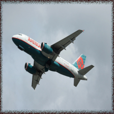
(a) airliner

(b) wing

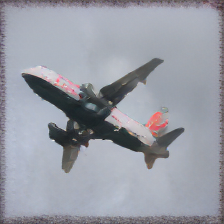
(c) shuttle

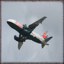
(d) warplane

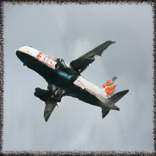
(e) wing

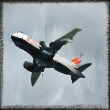
(f) warplane

(g) warplane

(h) tram

(i) prison

(j) crib

(k) vending

(l) chest

(m) school bus

(n) tram

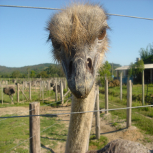
(o) ostrich

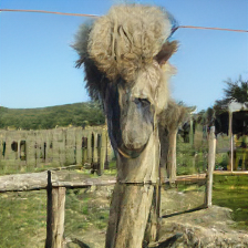
(p) dromedary

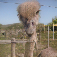
(q) llama

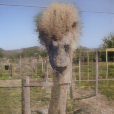
(r) poodle

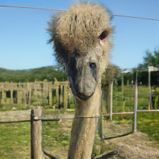
(s) llama

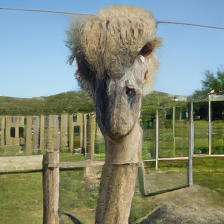
(t) dromedary

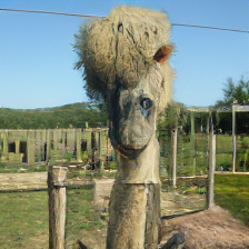
(u) llama

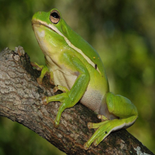
(v) tree frog

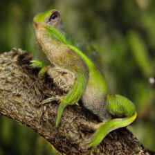
(w) mamba

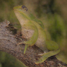
(x) greenlizard

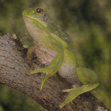
(y) greenlizard

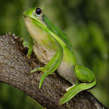
(z) greenlizard

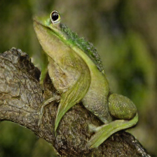
(aa) chameleon

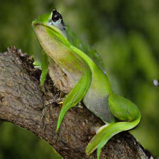
(ab) anole

(ac) washer

(ad) speaker

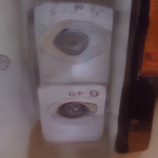
(ae) iPod

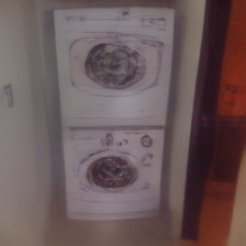
(af) microwave

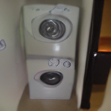
(ag) remote

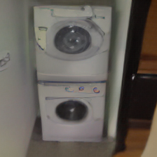
(ah) iPod

(ai) speaker

Figure 4: Visualization of the images generated by our system in evaluating the common corruption robust model, with the original image shown (left image of each row). The caption for each image is either the original label or the predicted label by the corresponding model. The evaluated models are SIN, ANT, ANT+SIN, Augmix, DeepAug and DeepAug+AM from left to right.

In Figure 4, we provide additional perturbed images generated according to each model. We have similar observations to Section 4.3. First, the generated perturbed images exhibit diversity that many other superficial factors of the data would be covered, i.e., texture, shape and styles. Second, our method could recognize the model properties, and automatically generate those hard perturbed images to complete the evaluation.

In addition, the generated images show a reasonable transferability in Table 6, indicating tha our method can be potentially used in a broader scope: we can also leverage the method to generate a static set of images and set a benchmark dataset to help the development of robustness methods. Therefore, we also offer two static benchmarks in supplementary materials that are generated based on CNN architecture, i.e., ConvNext and transformer variant, i.e., ViT, respectively.

We notice that some generated images look unnatural, as the generated images being realistic is not part of the optimization function. We acknowledge that making the generated images appear more natural will be a further desideratum, as this contributes to enhancing the human-perceptible interpretability.

Nonetheless, the current research agenda of the robustness evaluation community is still to encourage the evaluation to expose the model’s weakness, such as to expose and eliminate the model’s learning of spurious correlation in rare cases.

Similar evidence can be found in (Xiao et al., 2023), where the authors utilize masked images as counterfactual samples for robust fine-tuning. In this paper, the authors argue that masked images can break the spurious correlation between features and labels that may degrade OOD robustness, and that feature-based distillation with the pre-trained model on these counterfactual samples can achieve a better trade-off between IID and OOD performance. According to our second desideratum, our generated counterfactual images might also look unnatural. However, although it appears unnatural, it is beneficial in uncovering and eliminating spurious correlations for enhancing the model robustness.

References

- Bai et al. (2021) Yutong Bai, Jieru Mei, Alan L Yuille, and Cihang Xie. Are transformers more robust than cnns? Advances in Neural Information Processing Systems, 34:26831–26843, 2021.
- Ballester & Araujo (2016) Pedro Ballester and Ricardo Matsumura Araujo. On the performance of googlenet and alexnet applied to sketches. In Thirtieth AAAI Conference on Artificial Intelligence, 2016.
- Bareinboim et al. (2020) Elias Bareinboim, Juan D Correa, Duligur Ibeling, and Thomas Icard. On pearl’s hierarchy and the foundations of causal inference. ACM Special Volume in Honor of Judea Pearl (provisional title), 2(3):4, 2020.
- Ben-David et al. (2007) Shai Ben-David, John Blitzer, Koby Crammer, and Fernando Pereira. Analysis of representations for domain adaptation. In Advances in neural information processing systems, pp. 137–144, 2007.
- Ben-David et al. (2010) Shai Ben-David, John Blitzer, Koby Crammer, Alex Kulesza, Fernando Pereira, and Jennifer Wortman Vaughan. A theory of learning from different domains. Machine learning, 79(1-2):151–175, 2010.
- Bose et al. (2023) Digbalay Bose, Rajat Hebbar, Krishna Somandepalli, Haoyang Zhang, Yin Cui, Kree Cole-McLaughlin, Huisheng Wang, and Shrikanth Narayanan. Movieclip: Visual scene recognition in movies. In Proceedings of the IEEE/CVF Winter Conference on Applications of Computer Vision, pp. 2083–2092, 2023.
- Brendel & Bethge (2019) Wieland Brendel and Matthias Bethge. Approximating cnns with bag-of-local-features models works surprisingly well on imagenet. arXiv preprint arXiv:1904.00760, 2019.
- Carlini et al. (2019) Nicholas Carlini, Anish Athalye, Nicolas Papernot, Wieland Brendel, Jonas Rauber, Dimitris Tsipras, Ian Goodfellow, Aleksander Madry, and Alexey Kurakin. On evaluating adversarial robustness. arXiv preprint arXiv:1902.06705, 2019.
- Chen et al. (2021) Zhengsu Chen, Lingxi Xie, Jianwei Niu, Xuefeng Liu, Longhui Wei, and Qi Tian. Visformer: The vision-friendly transformer. In Proceedings of the IEEE/CVF International Conference on Computer Vision, pp. 589–598, 2021.
- Chu et al. (2021) Xiangxiang Chu, Zhi Tian, Yuqing Wang, Bo Zhang, Haibing Ren, Xiaolin Wei, Huaxia Xia, and Chunhua Shen. Twins: Revisiting the design of spatial attention in vision transformers. Advances in Neural Information Processing Systems, 34, 2021.
- Croce et al. (2020) Francesco Croce, Maksym Andriushchenko, Vikash Sehwag, Edoardo Debenedetti, Nicolas Flammarion, Mung Chiang, Prateek Mittal, and Matthias Hein. Robustbench: a standardized adversarial robustness benchmark. arXiv preprint arXiv:2010.09670, 2020.
- D’Amour et al. (2020) Alexander D’Amour, Katherine Heller, Dan Moldovan, Ben Adlam, Babak Alipanahi, Alex Beutel, Christina Chen, Jonathan Deaton, Jacob Eisenstein, Matthew D Hoffman, et al. Underspecification presents challenges for credibility in modern machine learning. arXiv preprint arXiv:2011.03395, 2020.
- Debenedetti et al. (2022) Edoardo Debenedetti, Vikash Sehwag, and Prateek Mittal. A light recipe to train robust vision transformers. arXiv preprint arXiv:2209.07399, 2022.
- Defazio et al. (2014) Aaron Defazio, Francis Bach, and Simon Lacoste-Julien. Saga: A fast incremental gradient method with support for non-strongly convex composite objectives. Advances in neural information processing systems, 27, 2014.
- Deng et al. (2009) Jia Deng, Wei Dong, Richard Socher, Li-Jia Li, Kai Li, and Li Fei-Fei. Imagenet: A large-scale hierarchical image database. In 2009 IEEE conference on computer vision and pattern recognition, pp. 248–255. Ieee, 2009.
- Dhariwal & Nichol (2021) Prafulla Dhariwal and Alexander Nichol. Diffusion models beat gans on image synthesis. Advances in Neural Information Processing Systems, 34:8780–8794, 2021.
- Dosovitskiy et al. (2020) Alexey Dosovitskiy, Lucas Beyer, Alexander Kolesnikov, Dirk Weissenborn, Xiaohua Zhai, Thomas Unterthiner, Mostafa Dehghani, Matthias Minderer, Georg Heigold, Sylvain Gelly, et al. An image is worth 16x16 words: Transformers for image recognition at scale. arXiv preprint arXiv:2010.11929, 2020.
- Duda et al. (1973) Richard O Duda, Peter E Hart, and David G Stork. Pattern classification and scene analysis, volume 3. Wiley New York, 1973.
- Edwards (2019) Chris Edwards. Malevolent machine learning. Commun. ACM, 62(12):13–15, nov 2019. ISSN 0001-0782.
- Engstrom et al. (2019) Logan Engstrom, Andrew Ilyas, Shibani Santurkar, Dimitris Tsipras, Brandon Tran, and Aleksander Madry. Adversarial robustness as a prior for learned representations. arXiv preprint arXiv:1906.00945, 2019.
- Esser et al. (2021) Patrick Esser, Robin Rombach, and Bjorn Ommer. Taming transformers for high-resolution image synthesis. In Proceedings of the IEEE/CVF Conference on Computer Vision and Pattern Recognition, pp. 12873–12883, 2021.
- Friedman et al. (2001) Jerome Friedman, Trevor Hastie, Robert Tibshirani, et al. The elements of statistical learning, volume 1. Springer series in statistics New York, 2001.
- Gatys et al. (2015) Leon Gatys, Alexander S Ecker, and Matthias Bethge. Texture synthesis using convolutional neural networks. Advances in neural information processing systems, 28, 2015.
- Gatys et al. (2017) Leon A Gatys, Alexander S Ecker, and Matthias Bethge. Texture and art with deep neural networks. Current opinion in neurobiology, 46:178–186, 2017.
- Geirhos et al. (2019) Robert Geirhos, Patricia Rubisch, Claudio Michaelis, Matthias Bethge, Felix A. Wichmann, and Wieland Brendel. Imagenet-trained CNNs are biased towards texture; increasing shape bias improves accuracy and robustness. In International Conference on Learning Representations, 2019.
- Goodfellow et al. (2015) Ian J Goodfellow, Jonathon Shlens, and Christian Szegedy. Explaining and harnessing adversarial examples (2014). In International Conference on Learning Representations, 2015.
- Gulrajani & Lopez-Paz (2020) Ishaan Gulrajani and David Lopez-Paz. In search of lost domain generalization. arXiv preprint arXiv:2007.01434, 2020.
- Guo et al. (2022) Jiayan Guo, Peiyan Zhang, Chaozhuo Li, Xing Xie, Yan Zhang, and Sunghun Kim. Evolutionary preference learning via graph nested gru ode for session-based recommendation. In Proceedings of the 31st ACM International Conference on Information & Knowledge Management, pp. 624–634, 2022.
- Hazami et al. (2022) Louay Hazami, Rayhane Mama, and Ragavan Thurairatnam. Efficient-vdvae: Less is more. arXiv preprint arXiv:2203.13751, 2022.
- He et al. (2015) Kaiming He, Xiangyu Zhang, Shaoqing Ren, and Jian Sun. Delving deep into rectifiers: Surpassing human-level performance on imagenet classification. In Proceedings of the IEEE international conference on computer vision, pp. 1026–1034, 2015.
- He et al. (2016a) Kaiming He, Xiangyu Zhang, Shaoqing Ren, and Jian Sun. Deep residual learning for image recognition. In Proceedings of the IEEE conference on computer vision and pattern recognition, pp. 770–778, 2016a.
- He et al. (2016b) Kaiming He, Xiangyu Zhang, Shaoqing Ren, and Jian Sun. Identity mappings in deep residual networks. In European conference on computer vision, pp. 630–645. Springer, 2016b.
- Hendrycks & Dietterich (2019) Dan Hendrycks and Thomas Dietterich. Benchmarking neural network robustness to common corruptions and perturbations. arXiv preprint arXiv:1903.12261, 2019.
- Hendrycks et al. (2019) Dan Hendrycks, Norman Mu, Ekin D Cubuk, Barret Zoph, Justin Gilmer, and Balaji Lakshminarayanan. Augmix: A simple data processing method to improve robustness and uncertainty. arXiv preprint arXiv:1912.02781, 2019.
- Hendrycks et al. (2021a) Dan Hendrycks, Steven Basart, Norman Mu, Saurav Kadavath, Frank Wang, Evan Dorundo, Rahul Desai, Tyler Zhu, Samyak Parajuli, Mike Guo, et al. The many faces of robustness: A critical analysis of out-of-distribution generalization. In Proceedings of the IEEE/CVF International Conference on Computer Vision, pp. 8340–8349, 2021a.
- Hendrycks et al. (2021b) Dan Hendrycks, Kevin Zhao, Steven Basart, Jacob Steinhardt, and Dawn Song. Natural adversarial examples. In Proceedings of the IEEE/CVF Conference on Computer Vision and Pattern Recognition, pp. 15262–15271, 2021b.
- Howard et al. (2017) Andrew G Howard, Menglong Zhu, Bo Chen, Dmitry Kalenichenko, Weijun Wang, Tobias Weyand, Marco Andreetto, and Hartwig Adam. Mobilenets: Efficient convolutional neural networks for mobile vision applications. arXiv preprint arXiv:1704.04861, 2017.
- Huang et al. (2017) Gao Huang, Zhuang Liu, Laurens Van Der Maaten, and Kilian Q Weinberger. Densely connected convolutional networks. In Proceedings of the IEEE conference on computer vision and pattern recognition, pp. 4700–4708, 2017.
- Kingma & Welling (2013) Diederik P Kingma and Max Welling. Auto-encoding variational bayes. arXiv preprint arXiv:1312.6114, 2013.
- Koh et al. (2021) Pang Wei Koh, Shiori Sagawa, Sang Michael Xie, Marvin Zhang, Akshay Balsubramani, Weihua Hu, Michihiro Yasunaga, Richard Lanas Phillips, Irena Gao, Tony Lee, et al. Wilds: A benchmark of in-the-wild distribution shifts. In International Conference on Machine Learning, pp. 5637–5664. PMLR, 2021.
- Krizhevsky et al. (2009) Alex Krizhevsky, Geoffrey Hinton, et al. Learning multiple layers of features from tiny images. 2009.
- LeCun et al. (1998) Yann LeCun, Léon Bottou, Yoshua Bengio, and Patrick Haffner. Gradient-based learning applied to document recognition. Proceedings of the IEEE, 86(11):2278–2324, 1998.
- Lei et al. (2023) Yuxuan Lei, Xiaolong Chen, Defu Lian, Peiyan Zhang, Jianxun Lian, Chaozhuo Li, and Xing Xie. Practical content-aware session-based recommendation: Deep retrieve then shallow rank. In Amazon KDD Cup 2023 Workshop, 2023.
- Li et al. (2017) Da Li, Yongxin Yang, Yi-Zhe Song, and Timothy M Hospedales. Deeper, broader and artier domain generalization. In Proceedings of the IEEE international conference on computer vision, pp. 5542–5550, 2017.
- Liu et al. (2023) Xihui Liu, Dong Huk Park, Samaneh Azadi, Gong Zhang, Arman Chopikyan, Yuxiao Hu, Humphrey Shi, Anna Rohrbach, and Trevor Darrell. More control for free! image synthesis with semantic diffusion guidance. In Proceedings of the IEEE/CVF Winter Conference on Applications of Computer Vision, pp. 289–299, 2023.
- Liu et al. (2021) Ze Liu, Yutong Lin, Yue Cao, Han Hu, Yixuan Wei, Zheng Zhang, Stephen Lin, and Baining Guo. Swin transformer: Hierarchical vision transformer using shifted windows. In Proceedings of the IEEE/CVF International Conference on Computer Vision, pp. 10012–10022, 2021.
- Liu et al. (2022) Zhuang Liu, Hanzi Mao, Chao-Yuan Wu, Christoph Feichtenhofer, Trevor Darrell, and Saining Xie. A convnet for the 2020s. arXiv preprint arXiv:2201.03545, 2022.
- Locatello et al. (2019) Francesco Locatello, Stefan Bauer, Mario Lucic, Gunnar Raetsch, Sylvain Gelly, Bernhard Schölkopf, and Olivier Bachem. Challenging common assumptions in the unsupervised learning of disentangled representations. In international conference on machine learning, pp. 4114–4124. PMLR, 2019.
- Madry et al. (2017) Aleksander Madry, Aleksandar Makelov, Ludwig Schmidt, Dimitris Tsipras, and Adrian Vladu. Towards deep learning models resistant to adversarial attacks. arXiv preprint arXiv:1706.06083, 2017.
- Mahajan et al. (2019) Divyat Mahajan, Chenhao Tan, and Amit Sharma. Preserving causal constraints in counterfactual explanations for machine learning classifiers. arXiv preprint arXiv:1912.03277, 2019.
- Mao et al. (2022a) Chengzhi Mao, Scott Geng, Junfeng Yang, Xin Wang, and Carl Vondrick. Understanding zero-shot adversarial robustness for large-scale models. arXiv preprint arXiv:2212.07016, 2022a.
- Mao et al. (2022b) Xiaofeng Mao, Yuefeng Chen, Ranjie Duan, Yao Zhu, Gege Qi, Xiaodan Li, Rong Zhang, Hui Xue, et al. Enhance the visual representation via discrete adversarial training. Advances in Neural Information Processing Systems, 35:7520–7533, 2022b.
- Marcos et al. (2016) Diego Marcos, Michele Volpi, and Devis Tuia. Learning rotation invariant convolutional filters for texture classification. In 2016 23rd International Conference on Pattern Recognition (ICPR), pp. 2012–2017. IEEE, 2016.
- Menon et al. (2022) Sachit Menon, Ishaan Preetam Chandratreya, and Carl Vondrick. Task bias in vision-language models. arXiv preprint arXiv:2212.04412, 2022.
- Muandet et al. (2013) Krikamol Muandet, David Balduzzi, and Bernhard Schölkopf. Domain generalization via invariant feature representation. In International Conference on Machine Learning, pp. 10–18, 2013.
- Nangia & Bowman (2019) Nikita Nangia and Samuel R Bowman. Human vs. muppet: A conservative estimate of human performance on the glue benchmark. arXiv preprint arXiv:1905.10425, 2019.
- Nichol & Dhariwal (2021) Alexander Quinn Nichol and Prafulla Dhariwal. Improved denoising diffusion probabilistic models. In International Conference on Machine Learning, pp. 8162–8171. PMLR, 2021.
- Orhan (2019) A Emin Orhan. Robustness properties of facebook’s resnext wsl models. arXiv preprint arXiv:1907.07640, 2019.
- Pearl (2009) Judea Pearl. Causality. Cambridge university press, 2009.
- Radford et al. (2021) Alec Radford, Jong Wook Kim, Chris Hallacy, Aditya Ramesh, Gabriel Goh, Sandhini Agarwal, Girish Sastry, Amanda Askell, Pamela Mishkin, Jack Clark, et al. Learning transferable visual models from natural language supervision. arXiv preprint arXiv:2103.00020, 2021.
- Recht et al. (2019) Benjamin Recht, Rebecca Roelofs, Ludwig Schmidt, and Vaishaal Shankar. Do imagenet classifiers generalize to imagenet? In International Conference on Machine Learning, pp. 5389–5400. PMLR, 2019.
- Rezende et al. (2014) Danilo Jimenez Rezende, Shakir Mohamed, and Daan Wierstra. Stochastic backpropagation and approximate inference in deep generative models. In International conference on machine learning, pp. 1278–1286. PMLR, 2014.
- Rozsa et al. (2016) Andras Rozsa, Manuel Günther, and Terrance E Boult. Are accuracy and robustness correlated. In 2016 15th IEEE international conference on machine learning and applications (ICMLA), pp. 227–232. IEEE, 2016.
- (64) Evgenia Rusak, Lukas Schott, Roland Zimmermann, Julian Bitterwolfb, Oliver Bringmann, Matthias Bethge, and Wieland Brendel. Increasing the robustness of dnns against im-age corruptions by playing the game of noise.
- Russakovsky et al. (2015) Olga Russakovsky, Jia Deng, Hao Su, Jonathan Krause, Sanjeev Satheesh, Sean Ma, Zhiheng Huang, Andrej Karpathy, Aditya Khosla, Michael Bernstein, et al. Imagenet large scale visual recognition challenge. International journal of computer vision, 115(3):211–252, 2015.
- Salimans et al. (2016) Tim Salimans, Ian Goodfellow, Wojciech Zaremba, Vicki Cheung, Alec Radford, and Xi Chen. Improved techniques for training gans. Advances in neural information processing systems, 29, 2016.
- Santurkar et al. (2019) Shibani Santurkar, Dimitris Tsipras, Brandon Tran, Andrew Ilyas, Logan Engstrom, and Aleksander Madry. Image synthesis with a single (robust) classifier. arXiv preprint arXiv:1906.09453, 2019.
- Sauer et al. (2022) Axel Sauer, Katja Schwarz, and Andreas Geiger. Stylegan-xl: Scaling stylegan to large diverse datasets. In ACM SIGGRAPH 2022 Conference Proceedings, pp. 1–10, 2022.
- Schneider et al. (2020) Steffen Schneider, Evgenia Rusak, Luisa Eck, Oliver Bringmann, Wieland Brendel, and Matthias Bethge. Improving robustness against common corruptions by covariate shift adaptation. Advances in Neural Information Processing Systems, 33:11539–11551, 2020.
- Simonyan & Zisserman (2014) Karen Simonyan and Andrew Zisserman. Very deep convolutional networks for large-scale image recognition. arXiv preprint arXiv:1409.1556, 2014.
- Sohl-Dickstein et al. (2015) Jascha Sohl-Dickstein, Eric Weiss, Niru Maheswaranathan, and Surya Ganguli. Deep unsupervised learning using nonequilibrium thermodynamics. In International Conference on Machine Learning, pp. 2256–2265. PMLR, 2015.
- Szegedy et al. (2013) Christian Szegedy, Wojciech Zaremba, Ilya Sutskever, Joan Bruna, Dumitru Erhan, Ian Goodfellow, and Rob Fergus. Intriguing properties of neural networks. arXiv preprint arXiv:1312.6199, 2013.
- Szegedy et al. (2015) Christian Szegedy, Wei Liu, Yangqing Jia, Pierre Sermanet, Scott Reed, Dragomir Anguelov, Dumitru Erhan, Vincent Vanhoucke, and Andrew Rabinovich. Going deeper with convolutions. In Proceedings of the IEEE conference on computer vision and pattern recognition, pp. 1–9, 2015.
- Tan & Le (2019) Mingxing Tan and Quoc Le. Efficientnet: Rethinking model scaling for convolutional neural networks. In International Conference on Machine Learning, pp. 6105–6114. PMLR, 2019.
- Taori et al. (2020) Rohan Taori, Achal Dave, Vaishaal Shankar, Nicholas Carlini, Benjamin Recht, and Ludwig Schmidt. Measuring robustness to natural distribution shifts in image classification. Advances in Neural Information Processing Systems, 33:18583–18599, 2020.
- Touvron et al. (2021) Hugo Touvron, Matthieu Cord, Matthijs Douze, Francisco Massa, Alexandre Sablayrolles, and Hervé Jégou. Training data-efficient image transformers & distillation through attention. In International Conference on Machine Learning, pp. 10347–10357. PMLR, 2021.
- Tsipras et al. (2018) Dimitris Tsipras, Shibani Santurkar, Logan Engstrom, Alexander Turner, and Aleksander Madry. Robustness may be at odds with accuracy. arXiv preprint arXiv:1805.12152, 2018.
- Wang et al. (2019) Haohan Wang, Songwei Ge, Eric P Xing, and Zachary C Lipton. Learning robust global representations by penalizing local predictive power. arXiv preprint arXiv:1905.13549, 2019.
- Wang et al. (2020a) Haohan Wang, Zeyi Huang, Xindi Wu, and Eric P Xing. Squared norm as consistency loss for leveraging augmented data to learn robust and invariant representations. arXiv preprint arXiv:2011.13052, 2020a.
- Wang et al. (2020b) Haohan Wang, Xindi Wu, Zeyi Huang, and Eric P Xing. High-frequency component helps explain the generalization of convolutional neural networks. In Proceedings of the IEEE/CVF Conference on Computer Vision and Pattern Recognition, pp. 8684–8694, 2020b.
- Wang et al. (2020c) Haohan Wang, Peiyan Zhang, and Eric P Xing. Word shape matters: Robust machine translation with visual embedding. arXiv preprint arXiv:2010.09997, 2020c.
- Wang et al. (2021) Haohan Wang, Zeyi Huang, Hanlin Zhang, and Eric Xing. Toward learning human-aligned cross-domain robust models by countering misaligned features. arXiv preprint arXiv:2111.03740, 2021.
- Wang et al. (2022a) Junyang Wang, Yi Zhang, and Jitao Sang. Fairclip: Social bias elimination based on attribute prototype learning and representation neutralization. arXiv preprint arXiv:2210.14562, 2022a.
- Wang et al. (2022b) Zeyu Wang, Yutong Bai, Yuyin Zhou, and Cihang Xie. Can cnns be more robust than transformers? arXiv preprint arXiv:2206.03452, 2022b.
- Wightman (2019) Ross Wightman. Pytorch image models. https://github.com/rwightman/pytorch-image-models, 2019.
- Wu et al. (2023) Shirley Wu, Mert Yuksekgonul, Linjun Zhang, and James Zou. Discover and cure: Concept-aware mitigation of spurious correlation. arXiv preprint arXiv:2305.00650, 2023.
- Xia et al. (2021) Kevin Xia, Kai-Zhan Lee, Yoshua Bengio, and Elias Bareinboim. The causal-neural connection: Expressiveness, learnability, and inference. Advances in Neural Information Processing Systems, 34, 2021.
- Xiao et al. (2023) Yao Xiao, Ziyi Tang, Pengxu Wei, Cong Liu, and Liang Lin. Masked images are counterfactual samples for robust fine-tuning. arXiv preprint arXiv:2303.03052, 2023.
- Xie et al. (2020) Qizhe Xie, Minh-Thang Luong, Eduard Hovy, and Quoc V Le. Self-training with noisy student improves imagenet classification. In Proceedings of the IEEE/CVF conference on computer vision and pattern recognition, pp. 10687–10698, 2020.
- Ye et al. (2021) Nanyang Ye, Kaican Li, Lanqing Hong, Haoyue Bai, Yiting Chen, Fengwei Zhou, and Zhenguo Li. Ood-bench: Benchmarking and understanding out-of-distribution generalization datasets and algorithms. arXiv preprint arXiv:2106.03721, 2021.
- Yu et al. (2018) Fisher Yu, Dequan Wang, Evan Shelhamer, and Trevor Darrell. Deep layer aggregation. In Proceedings of the IEEE conference on computer vision and pattern recognition, pp. 2403–2412, 2018.
- Yun et al. (2019) Sangdoo Yun, Dongyoon Han, Seong Joon Oh, Sanghyuk Chun, Junsuk Choe, and Youngjoon Yoo. Cutmix: Regularization strategy to train strong classifiers with localizable features. In Proceedings of the IEEE/CVF international conference on computer vision, pp. 6023–6032, 2019.
- Zhang et al. (2017) Hongyi Zhang, Moustapha Cisse, Yann N Dauphin, and David Lopez-Paz. mixup: Beyond empirical risk minimization. arXiv preprint arXiv:1710.09412, 2017.
- Zhang & Kim (2023) Peiyan Zhang and Sunghun Kim. A survey on incremental update for neural recommender systems. arXiv preprint arXiv:2303.02851, 2023.
- Zhang et al. (2023a) Peiyan Zhang, Jiayan Guo, Chaozhuo Li, Yueqi Xie, Jae Boum Kim, Yan Zhang, Xing Xie, Haohan Wang, and Sunghun Kim. Efficiently leveraging multi-level user intent for session-based recommendation via atten-mixer network. In Proceedings of the Sixteenth ACM International Conference on Web Search and Data Mining, pp. 168–176, 2023a.
- Zhang et al. (2023b) Peiyan Zhang, Yuchen Yan, Chaozhuo Li, Senzhang Wang, Xing Xie, Guojie Song, and Sunghun Kim. Continual learning on dynamic graphs via parameter isolation. arXiv preprint arXiv:2305.13825, 2023b.
- Zhang et al. (2023c) Qiming Zhang, Yufei Xu, Jing Zhang, and Dacheng Tao. Vitaev2: Vision transformer advanced by exploring inductive bias for image recognition and beyond. International Journal of Computer Vision, pp. 1–22, 2023c.
- Zhang (2019) Richard Zhang. Making convolutional networks shift-invariant again. In International conference on machine learning, pp. 7324–7334. PMLR, 2019.
- Zhang & Zhu (2019) Tianyuan Zhang and Zhanxing Zhu. Interpreting adversarially trained convolutional neural networks. In International Conference on Machine Learning, pp. 7502–7511. PMLR, 2019.
- Zhong et al. (2020) Zhun Zhong, Liang Zheng, Guoliang Kang, Shaozi Li, and Yi Yang. Random erasing data augmentation. In Proceedings of the AAAI conference on artificial intelligence, volume 34, pp. 13001–13008, 2020.
- Zhou et al. (2022a) Daquan Zhou, Zhiding Yu, Enze Xie, Chaowei Xiao, Animashree Anandkumar, Jiashi Feng, and Jose M Alvarez. Understanding the robustness in vision transformers. In International Conference on Machine Learning, pp. 27378–27394. PMLR, 2022a.
- Zhou et al. (2022b) Kankan Zhou, Yibin LAI, and Jing Jiang. Vlstereoset: A study of stereotypical bias in pre-trained vision-language models. Association for Computational Linguistics, 2022b.