Superconducting Quantum Circuits in the light of
Dirac’s Constraint Analysis Framework

The paper is dedicated to the memory of Professor Roman Jackiw, who apart from working in diverse branches of theoretical physics, has contributed significantly in quantization of constraint systems.

Abstract: In this work we introduce a new framework - Dirac’s Hamiltonian formalism of constraint systems - to study different types of Superconducting Quantum Circuits (SQC) in a unified and unambiguous way. The Lagrangian of a SQC reveals the constraints, that are classified in a Hamiltonian framework, such that redundant variables can be removed to isolate the canonical degrees of freedom for subsequent quantization of the Dirac Brackets via a generalized Correspondence Principle. This purely algebraic approach makes the application of concepts such as graph theory, null vector, loop charge, etc that are in vogue, (each for a specific type of circuit), completely redundant.

I Introduction

Superconducting Quantum Circuits (SQC), in recent times, are described with extreme accuracy by the theory of Circuit Quantization. Whereas qubits are described by microscopic elements, such as electrons, atoms, ions, and photons, SQCs are constructed out of macroscopic entities such as electrical (LC) oscillator, connected by everyday objects like metallic wires and plates. The SQC works on superconductivity, which is the flow of electrical fluid without friction through the metal at low temperature (below the superconducting phase transition), and the Josephson effect, that introduces nonlinearity without dissipation or dephasing. The collective motion of the electron fluid in SQC is described by the flux threading the inductor, which acts as the center-of-mass position in a mass-spring mechanical oscillator. It is quite well known that conventional inductor-capacitor-resistance (LCR) circuit with batteries has a Lagrangian description with degrees of freedom being either magnetic fluxes or electric charges in the circuit. Interestingly enough, similar principle works for the construction of a Lagrangian for SQC as well with introduction of nonlinear circuit elements (such as Josephson junctions or quantum phase slips). However, and this is where our formalism enters into the play, it is possible to build circuits where a Lagrangian exists but its conventional analysis (Lagrange equations of motion) fails to generate the correct dynamics because the system can have constraints. In SQC theory a Hamiltonian framework is favoured since it can yield the quantum commutators from classical Poisson brackets via Correspondence Principle.

We quote from a very recent paper by Osborne et.al. sym ”For example, the number of degrees of freedom is not equal to the number of Josephson Junctions or Quantum Phase Slips; worse, the fluxes and charges across the different elements may not be conjugate pairs. Understanding how to even identify the dynamical degrees of freedom, let alone quantize the circuit, is an open problem”. The stumbling block in Quantum Circuit analysis in conventional Condensed Matter framework is pretty clear - proper identification of the canonical Degrees Of Freedom (DOF), (essential to implement quantization prescription), is not always straightforward to find directly from the Lagrangian. This paper sym has advocated sophisticated mathematical machinery such as graph theory in the study of SQC. Another work dual uses loop charges in the analysis. In fact existing literature in this context have put forward different formalisms for different types of circuits and there appears to be no unified unambiguous framework. Indeed, it is unfortunate that our colleagues are unaware of the very well established scheme of constraint analysis in Dirac’s Hamiltonian framework dir . As we discuss with explicit examples in rest of the paper, Dirac’s formalism is perfectly suited for the study of any form of SQC (described by a Lagrangian). At the end of the systematic analysis the canonical DOFs are identified unambiguously. But that is not all! If one has a specific form of quantum brackets in mind, one can construct a Lagrangian that will generate such algebra and subsequently try to implement the corresponding SQC. In passing we note that Symplectic Geometry formulation has also been used sym1 ; sym but once again from physics perspective, it is more convenient to follow the Faddeev-Jackiw symplectic framework fad .

SQCs play an essential role in the present era of actively pursuing improvements in Quantum Computation (and Quantum Computers) qcomp and designing of qubits have been diversified in to other design variations, such as the quantronium quant , transmon trans , fluxonium flux , and “hybrid” hybrid qubits, all of which are less sensitive to decoherence mechanisms thereby improving performance. Quantum effects at the macroscopic level are manifested in the field of circuit quantum electrodynamics sqed where SQC as qubits interact strongly and controllably with microwave photons.

II Constraint analysis in a nutshell

We quickly recapitulate the salient features, (that will be particularly used here), of Dirac’s Hamiltonian formulation of constraint analysis. For a generic Lagrangian $L(q_{i},\dot{q}_{i})$, canonical momenta are defined as

$$p_{i}=(\partial L)/(\partial\dot{q}_{i})$$ (1)

that satisfy canonical Poisson Brackets (PB) $\{q_{i},p_{j}\}=\delta_{ij},~{}\{q_{i},q_{j}\}=\{p_{i},p_{j}\}=0$. The equations of the form

$$\chi_{k}=p_{k}-f_{k}(q_{j})\approx 0$$ (2)

that do not contain $\dot{q}_{i}$ are treated as constraints. Next the extended form Hamiltonian, taking into account the constraints, is given by

$$H_{E}=p_{i}\dot{q}_{i}-L+\alpha_{k}\chi_{k}$$ (3)

where $\alpha_{k}$ are Lagrange arbitrary multipliers. Time persistence of $\chi_{k}$, given by

$$\dot{\chi}_{k}=\{\chi_{k},H_{E}\}\approx 0$$ (4)

can give rise to further new constraints or in some cases some of the $\alpha_{k}$ can be determined (thus not generating new constraints). Note that ”$\approx$” is a weak equality, modulo constraints, and can not be used directly, in contrast to ”$=$” strong equality (that appears later) that can be used directly on dynamical variables. This process will continue until no further constraints are generated. Once the full set of linearly independent constraints are determined the First Class Constraints (FCC), (associated with gauge invariance), $\psi_{r}$ obeying $\{\psi_{r},\chi_{k}\}\approx 0$ for all $k$ are isolated. Rest of the constraints are named Second Class Constraints (SCC). These are used to compute the all important non-singular constraint matrix $\chi_{kl}=\{\chi_{k},\chi_{l}\}$. The SCCs can be used as strong relations to eliminate some of the DOF provided Dirac brackets (DB), for two generic variables $A,B$, are used,

$$\{A,B\}_{DB}=\{A,B\}-\{A,\chi_{r}\}{\chi}_{rs}^{-1}\{\chi_{s},B\},$$ (5)

where ${\chi}_{rs}^{-1}{\chi}_{st}=\delta_{rt}$. Notice that $\{A,\chi_{r}\}_{DB}=0$ for any $A$ which justifies using $\chi_{r}=0$ so that each SCC $\chi_{r}$ removes one DOF. Thus finally one has the Hamiltonian comprising of a reduced number of variables and time evolution of $A$ is computed using DBs

$$\dot{A}=\{A,H\}_{DB}.$$ (6)

Notice that, under normal circumstances, there will be an even number of SCCs since the matrices $\chi$ and $\chi^{-1}$ are anti-symmetric and non-singular.

One still has the FCC which reveals gauge symmetry of the model. The FCCs, together with respective gauge fixing conditions, give rise to a further set of SCCs, further DBs, that will further reduce the number of DOF. It is important to note that each SCC can remove one DOF in phase space and each FCC can remove two DOF in phase space (because of its associated gauge condition) leading to the formula

$$({\text{number of physical DOF in phase space}})=({\text{total number of DOF in phase space}})$$

$$-(2\times({\text{number of FCC}})+1\times({\text{number of SCC}})).$$ (7)

Due to the freedom of choice in (allowed) gauge conditions there can be manifestly different but gauge equivalent models. This brief introduction of Dirac’s constraint analysis in Hamiltonian framework will suffice for the present work.

III Dirac Analysis of Inductively Shunted SQC:

One of the major operational models of Quantum computing is Quantum Circuits, that have straightforward analogy with classical computers: wires connecting gates that in turn manipulate qubits. The transformation performed by the gates are always reversible, contrary to classical computers.

For the present study we borrow a model from sym . Corresponding to the Quantum Circuit (QC) , Figure (1), the action is defined as

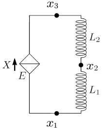
Figure 1: A circuit involving an inductively shunted island at $x_{2}$ sym .

$$L=X(\dot{x}_{3}-\dot{x}_{1})+Ecos(\frac{2\pi X}{2e})-\frac{1}{2L_{1}}(x_{1}-x_{2})^{2}-\frac{1}{2L_{2}}(x_{2}-x_{3})^{2}$$ (8)

$$P_{i}=\frac{\partial L}{\partial\dot{x}_{i}},~{}\pi=\frac{\partial L}{\partial\dot{X}}$$ (9)

$\{x_{i},P_{j}\}=\delta_{ij},~{}\{X,\pi\}=1$. Denoting constraints by $\chi_{i}$

$$\chi_{1}=P_{1}+X\approx 0,~{}\chi_{2}=P_{2}\approx 0,~{}\chi_{3}=P_{3}-X\approx 0,~{}\chi_{4}=\pi\approx 0$$ (10)

or equivalently a linear combination of them

$$\chi_{1}=P_{1}+P_{3}\approx 0,~{}\chi_{2}=P_{2}\approx 0,~{}\chi_{3}=P_{3}-X\approx 0,~{}\chi_{4}=\pi\approx 0$$ (11)

we define the extended Hamiltonian

$$H_{E}=-Ecos(\frac{2\pi P_{3}}{2e})+\frac{1}{2L_{1}}(x_{1}-x_{2})^{2}+\frac{1}{2L_{2}}(x_{2}-x_{3})^{2}+\sum_{i=1}^{4}\alpha_{i}\chi_{i}$$ (12)

where $\alpha_{i}$ are arbitrary multipliers. From requiring time invariance of the constraints $\dot{\chi_{i}}=\{\chi_{i},H_{E}\}\approx 0$, $\alpha_{3},\alpha_{4}$ are obtained from $\dot{\chi_{3}}=0,\dot{\chi_{4}}=0$ respectively.

Note the SCC pair $\chi_{3},\chi_{4}$ commutes with the other constraints and hence their Dirac Brackets can be calculated in the first stage. This does not induce any change in the brackets of the variables of interest.

Considering the remaining constraints we find that $\alpha_{1},\alpha_{2}$ can not be determined and a new constraint is generated

$$\dot{\chi}_{1}=\{\chi_{1},H\}=((L_{1}+L_{2})x_{2}-(L_{1}x_{3}+L_{2}x_{1}))/(L_{1}L_{2})\equiv\chi_{5}\approx 0,~{}\dot{\chi}_{2}=-\equiv\chi_{5}\approx 0.$$ (13)

It can be shown that $\Psi=\chi_{1}+\chi_{2}=P_{1}+P_{2}+P_{3}\approx 0$ is a FCC since it commutes with rest of the constraints $\chi_{1},\chi_{2},\chi_{5}$. Since $\dot{\Psi}=\{\Psi,H\}\approx 0$ the chain of constraints stops and there are no further constraints with

$$H=-Ecos(\frac{2\pi P_{3}}{2e})+\frac{1}{2L_{1}}(x_{1}-x_{2})^{2}+\frac{1}{2L_{2}}(x_{2}-x_{3})^{2}.$$ (14)

Since $\Psi$ is already considered as an FCC we can consider $\chi_{5}$ and either of $\chi_{1},\chi_{2}$ as the SCC pair. Let us choose the SCC pair $\chi_{2},\chi_{5}$ and use them strongly to obtain

$$H=-Ecos(\frac{2\pi P_{3}}{2e})+\frac{1}{2(L_{1}+L_{2})}(x_{1}-x_{3})^{2}$$ (15)

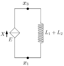
Figure 2: A dynamically equivalent circuit to figure 1 with the non-dynamical variables removed sym .

The brackets between $P_{3},x_{1},x_{3}$ are not affected. Notice that $\{P_{3},x_{1}-x_{3}\}=1$ is a canonical pair. This agrees with our DOF count since there are overall four SCC and one FCC yielding $8-(4\times 1+1\times 2)=2$ DOF in phase space or one DOF in configuration space. The corresponding SQC is shown in Figure 2.

Additional freedom revealed in Dirac analysis: We still have the FCC $\psi\approx 0$ for which we can choose a gauge constraint $\Theta=x_{1}\approx 0$, (such that $(\psi,\Theta)$ turns into an SCC pair), leading to

$$H=-Ecos(\frac{2\pi P_{3}}{2e})+\frac{1}{2(L_{1}+L_{2})}(x_{3})^{2}$$ (16)

with the reduced circuit, as in Figure (2). The above constitute two DOF in phase space (or a single DOF in configuration space). This is consistent with the number of constraints present. We started with $x_{1},x_{2},x_{3},X$ configuration space DOF giving rise to $4\times 2=8$ DOF in phase space. Our analysis has revealed that there are four SCCs each taking out one DOF in phase space and one FCC, which, together with its gauge fixing condition removing two more DOF in phase space, resulting in $8-6=2$ DOF in phase space, i.e. $x_{3},P_{3}$. We emphasize that in Dirac’s method, we have recovered identical result as sym but in a more direct and simple way.

As advertised earlier, we now show effect of the additional symmetry revealed in Dirac scheme related to the FCC since we can choose different gauge condition leading to different looking $H$. Let us choose

$$\Theta=ax_{1}+bx_{3}$$ (17)

for $a,b$ being arbitrary constants. This will lead to DBs

$$\{x_{1},P_{1}\}_{DB}=\frac{b}{a+b},~{}\{x_{1},P_{3}\}_{DB}=-\frac{b}{a+b},$$

$$\{x_{3},P_{3}\}_{DB}=\frac{a}{a+b},~{}\{x_{3},P_{1}\}_{DB}=-\frac{a}{a+b}$$ (18)

Using the gauge condition (17) $x_{1}=-\frac{b}{a}x_{3}$ we find

$$H=-Ecos(\frac{2\pi P_{3}}{2e})+\frac{1}{2(L_{1}+L_{2})}(\frac{a+b}{a})^{2}(x_{3})^{2}$$ (19)

and equations of motion

$$\dot{x}_{3}=\frac{a}{a+b}\frac{2\pi E}{2e}sin(\frac{2\pi P_{3}}{2e}),~{}\dot{P}_{3}=-\frac{a+b}{a}\frac{x_{3}}{L_{1}+L_{2}}$$ (20)

finally yielding

$$\ddot{x}_{3}=-(\frac{2\pi}{2e})^{2}\frac{E}{L_{1}+L_{2}}cos(\frac{2\pi P_{3}}{2e})x_{3}.$$ (21)

Note that (21) is gauge invariant as it is independent of $a,b$. Also notice that the bracket $\{x_{3},P_{3}\}_{DB}=\frac{a}{a+b}$ can be directly identified from the Lagrangian

$$L=\frac{a+b}{a}\dot{x}_{3}P_{3}+Ecos(\frac{2\pi P_{3}}{2e})+\frac{1}{2(L_{1}+L_{2})}(\frac{a+b}{a})^{2}(x_{3})^{2}$$ (22)

and in fact with a redefinition $\frac{a+b}{a}x\rightarrow x$ the system becomes trivially canonical.

IV Dirac Analysis of Capacitively Shunted SQC:

Let us quickly analyse a SQC with one of the three flux variables being connected to two capacitors as shown in Figure (3), along with a Josephson-junction element with energy $E$. It is worthwhile to emphasize the advantage of the unified approach in Dirac scheme since, as elaborated in sym , the inductively shunted model of Section III and capacitatively shunted model in this section, had to be treated quite differently. The inductively shunted islands corresponded to right null vectors of the symplectic form, while capacitatively shunted islands corresponded to the presence of a Noether charge in the circuit. However, within the Dirac formalism, pursued here, no such distinctions are made. Non-dynamical variables are removed by the use of constraints in exactly the same manner for either type of shunted islands.

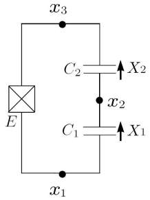
Figure 3: A circuit with a capacitive shunted island at $x_{2}$ sym .

The corresponding Lagrangian is sym

$$L=X_{1}(\dot{x}_{2}-\dot{x}_{1})+X_{2}(\dot{x}_{3}-\dot{x}_{2})+E\cos{\left(2\pi\frac{x_{1}-x_{3}}{x_{0}}\right)}-\frac{1}{2C_{1}}X_{1}^{2}-\frac{1}{2C_{2}}X_{2}^{2}.$$ (23)

The conjugate momenta are $p_{i}=\frac{\partial L}{\partial\dot{x}_{i}},P_{i}=\frac{\partial L}{\partial\dot{X}_{i}}$ With $\{x_{i},p_{j}\}=\delta_{ij},~{}\{X_{i},P_{j}\}=\delta_{ij}$. The constraints $\chi_{k}\approx 0$ are

$$\chi_{1}=p_{1}+X_{1},~{}\chi_{2}=p_{3}-X_{2},~{}\chi_{3}=p_{2}-X_{1}+X_{2},~{}\chi_{4}=P_{1},~{}\chi_{5}=P_{2}.$$ (24)

As mentioned before, for a discrete variable constraint system, odd number of SCCs are not possible. Here we find the combination $\Psi=\chi_{1}+\chi_{2}+\chi_{3}=p_{1}+p_{2}+p_{3}\approx 0$ commutes with all the constraints and is an FCC. Of the remaining four independent SCC note that $(\chi_{1},\chi_{4})$ and $(\chi_{2},\chi_{5})$ are mutually commuting SCC pairs; DBs can be constructed for the individual pairs separately.

Let us find the DOF count: there are four SCC and one FCC with $x_{1},x_{2},x_{3},X_{1},X_{2}$ ”coordinates” together with their momenta. Number of independent DOF is $5\times 2-(4\times 1+1\times 2)=4$; there are two full DOF in configuration space.

The Hamiltonian on constraint surface is written as

$$H=-Ecos\left(\frac{2\pi}{x_{0}}(x_{1}-x_{3})\right)+\frac{1}{2C_{1}}X_{1}^{2}+\frac{1}{2C_{2}}X_{2}^{2}$$ (25)

together with the two non-zero DBs

$$\{x_{1},X_{1}\}=1,~{}~{}\{x_{3},X_{2}\}=1.$$ (26)

The above behave as two independent canonical DOF. The equations of motion follow:

$$\dot{x}_{1}=\frac{X_{1}}{C_{1}},~{}\dot{X}_{1}=-\frac{2\pi E}{x_{0}}sin\left(\frac{2\pi}{x_{0}}(x_{1}-x_{3})\right),$$

$$\dot{x}_{3}=\frac{X_{2}}{C_{2}},~{}\dot{X}_{2}=+\frac{2\pi E}{x_{0}}sin\left(\frac{2\pi}{x_{0}}(x_{1}-x_{3})\right)$$ (27)

Defining $x_{1}-x_{3}=Q$ we find

$$\ddot{Q}=-(\frac{1}{C_{1}}+\frac{1}{C_{2}})\frac{2\pi E}{x_{0}}sin\left(\frac{2\pi}{x_{0}}Q\right).$$ (28)

Note that $d(X_{1}+X_{2})/dt=0\rightarrow~{}X_{1}+X_{2}$ is a conserved quantity and so the corresponding cyclic ”coordinate”, proportional to $x_{1}+x_{3}$ is absent. The equivalent circuit is a SQC with $C_{1}$ and $C_{2}$ in series combination. Once again we have obtained same results as sym , but using the identical analysis as earlier..

V Dirac Analysis of a ”Noncommutative” SQC

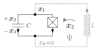
Figure 4: Idealized fluxonium circuit dual

Consider the circuit in Figure (4) and the corresponding Lagrangian, discussed in dual

$$L=\frac{C}{2}\dot{x}^{2}_{1}+\frac{L}{2}\dot{x}^{2}_{2}+Ecos(\frac{2\pi x_{1}}{A})-x_{2}\dot{x}_{1}+\dot{x}_{2}\Psi$$ (29)

with $\Psi$ an external source. In dual the authors have advocated a dual approach using loop charge representation to quantize the SQC. In the Dirac scheme this model is simple since clearly there are no (Hamiltonian) constraint.

Instead of solving the above we consider a slightly different model. Let us introduce a twist by considering a situation when $\dot{x}_{2}$ is small thereby neglecting $\dot{x}^{2}_{2}$ leading to

$$L=\frac{C}{2}\dot{x}^{2}_{1}+Ecos(\frac{2\pi x_{1}}{A})-x_{2}\dot{x}_{1}+\dot{x}_{2}\Psi.$$ (30)

We have a particular motivation of complicating the circuit by introducing a constraint. We will see that the resulting system has a non-trivial DB between the ”coordinates” $x_{1},x_{2}$, thus inducing a ”spatial” non-commutativity in the system — an analogue of spatial non-commutative quantum mechanics. From the canonical momenta $P_{1}=C\dot{x}_{1}-x_{2},~{}P_{2}=\Psi$, the Hamiltonian is

$$H=\frac{1}{2C}(P_{1}+x_{2})^{2}-Ecos(\frac{2\pi x_{1}}{A})$$ (31)

along with the constraint

$$\chi_{1}=P_{2}-\Psi.$$ (32)

$\dot{\chi}_{1}=\chi_{2}\approx 0$ generates a new constraint

$${\chi}_{2}=P_{1}+x_{2}.$$ (33)

The constraints $\chi_{1},\chi_{2}$ constitute an SCC pair, leading to the only non-zero DBs

$$\{x_{1},x_{2}\}=-1,~{}\{x_{1},P_{1}\}=1.$$ (34)

Therefore on the constraint surface $P_{1}+x_{2}=0$ (since it DBs between $\chi_{2}=P_{1}+x_{2}$ and any variable vanishes), and $H$ reduces to

$$H=-Ecos(\frac{2\pi x_{1}}{A}).$$ (35)

The equations of motion are

$$\dot{x}_{1}=\{x_{1},H\}=0,~{}\dot{x}_{2}=\{x_{2},H\}=-\frac{2\pi E}{A}sin(\frac{2\pi x_{1}}{A})$$ (36)

so that the first relation in (36) gives $x_{1}=C$, with $C$ a constant, and $\dot{x}_{2}=-\frac{2\pi E}{A}sin(\frac{2\pi x_{1}}{A})|_{x_{1}=C}=-\frac{2\pi E}{A}sin(\frac{2\pi C}{A})$, another constant.

Interestingly the symplectic structure (or kinetic term) in the action $x_{2}\dot{x}_{1}$ appears in condensed matter physics in well known Landau problem, i.e. a charged particle moving in $x_{1}-x_{2}$-plane, in a constant magnetic field perpendicular to the plane, with the condition that the magnetic field is large so that kinetic energy of the particle is negligible. This is a well-known example of a non-commutative quantum mechanical problem noncom .

VI Dirac Analysis of A Generic SQC

We consider a generic form of SQC (whose circuit representation needs to be addressed)

$$L=X(\dot{x}_{3}-\dot{x}_{1})+Ecos(\frac{2\pi X}{2e})-\frac{1}{2L_{1}}(x_{1}-x_{2})^{2}-\frac{1}{2L_{2}}(x_{2}-x_{3})^{2}+\lambda_{1}\dot{x}_{1}x_{3}+\lambda_{2}\dot{x}_{1}x_{2}+\lambda_{3}\dot{x}_{2}x_{3}.$$ (37)

Denoting constraints by $\chi_{i}$

$$\chi_{1}=P_{1}+P_{3}-\lambda_{1}x_{3}-\lambda_{2}x_{2}\approx 0,~{}\chi_{2}=P_{2}-\lambda_{3}x_{3}\approx 0,~{}\chi_{3}=P_{3}-X\approx 0,~{}\chi_{4}=\pi\approx 0$$ (38)

define extended Hamiltonian

$$H=-Ecos(\frac{2\pi P_{3}}{2e})+\frac{1}{2L_{1}}(x_{1}-x_{2})^{2}+\frac{1}{2L_{2}}(x_{2}-x_{3})^{2}+\sum_{i=1}^{4}\alpha_{i}\chi_{i}$$ (39)

A crucial difference between this and the previously discussed model is that here $\dot{\chi}_{i}\approx 0$ fixes all the $\alpha_{i}$, so there are no further constraints. Furthermore since the constraint matrix $\{\chi_{i},\chi_{j}\}$ is non-singular, $\chi_{i}$ comprises a set of four SCC and there are no FCC as in the previous case. Thus we should have $8-(4\times 1)=4$ DOF in phase space or two independent DOF in configuration space. Our subsequent analysis will show this to be the case.

The full set of DBs among ”coordinate” variables are given by

$$\{x_{1},x_{2}\}_{DB}=\frac{1}{\lambda_{2}-\lambda_{3}},~{}\{x_{1},x_{3}\}_{DB}=0,~{}\{x_{1},X\}_{DB}=\frac{\lambda_{3}}{\lambda_{2}-\lambda_{3}},$$

$$\{x_{2},x_{3}\}_{DB}=-\frac{1}{\lambda_{2}-\lambda_{3}},~{}\{x_{2},X\}_{DB}=-\frac{\lambda_{1}}{\lambda_{2}-\lambda_{3}},~{}\{x_{3},X\}_{DB}=\frac{\lambda_{2}}{\lambda_{2}-\lambda_{3}}$$ (40)

The significance of noncommutative quantum circuits is now clear since conventionally noncommutative quantum mechanics refers to models where spatial coordinates do not commute. Rest of the DBs are can also be computed in a straightforward way but for the present model these are not required. We can exploit the SCCs $\chi_{i}=0$ as strong relations to express the Hamiltonian as

$$H=-Ecos(\frac{2\pi X}{2e})+\frac{1}{2L_{1}}(x_{1}-x_{2})^{2}+\frac{1}{2L_{2}}(x_{2}-x_{3})^{2}+\sum_{i=1}^{4}\alpha_{i}\chi_{i}.$$ (41)

It is interesting to note that the under DB the DOFs $(Q_{1},P_{1})$ and $(Q_{2},P_{2})$ constitute two independent canonical degrees of freedom where

$$Q_{1}=(x_{3}-x_{1}),~{}P_{1}=X,~{}Q_{2}=x_{2}+\frac{\lambda_{1}}{\lambda_{3}}x_{1},~{}P_{2}=-\lambda_{2}x_{1}+\lambda_{3}x_{3},$$ (42)

with the only non-vanishing DBs being $\{Q_{1},P_{1}\}_{DB}=1,~{}\{Q_{2},P_{2}\}_{DB}=1$. This result agrees with our advertised DOF count.

Let us invert the relations (42)

$$x_{1}=\frac{\lambda_{3}-P_{2}}{\lambda_{2}-\lambda_{3}},~{}x_{2}=\frac{Q_{2}\lambda_{3}(\lambda_{2}-\lambda_{3})-\lambda_{1}(\lambda_{3}Q_{1}-P_{2})}{\lambda_{3}(\lambda_{2}-\lambda_{3})},~{}x_{3}=\frac{Q_{1}\lambda_{2}-P_{2}}{\lambda_{2}-\lambda_{3}},~{}X=P_{1}.$$ (43)

Keeping the unique noncommutative feature of the circuit intact let us consider a simplified model with $\lambda_{1}=\lambda_{2}=0,~{}\lambda_{3}=\lambda$ so that the Dirac algebra simplifies to

$$\{x_{1},x_{2}\}_{DB}=-\frac{1}{\lambda},~{}\{x_{1},x_{3}\}_{DB}=0,~{}\{x_{1},X\}_{DB}=-1,~{}\{x_{2},x_{3}\}_{DB}=\frac{1}{\lambda},$$

$$\{x_{2},X\}_{DB}=0,~{}\{x_{3},X\}_{DB}=0.$$ (44)

The Hamiltonian (35) is expressed in terms of canonical variables as

$$H=-Ecos(\frac{2\pi P_{1}}{2e})+\frac{1}{2L_{1}\lambda^{2}}(\lambda(Q_{1}+Q_{2})-P_{2})^{2}+\frac{1}{2L_{2}\lambda^{2}}(\lambda Q_{2}-P_{2})^{2}.$$ (45)

This will yield the equations of motion

$$\ddot{Q}_{1}=(\frac{2\pi}{2e})^{2}Ecos(\frac{2\pi P_{1}}{2e})(-\frac{Q_{1}+Q_{2}}{L_{1}}+\frac{P_{2}}{\lambda L_{1}}),~{}\ddot{Q}_{2}=-\frac{1}{L_{2}\lambda^{3}}(\frac{\lambda}{L_{1}}((Q_{1}+Q_{2})-P_{2}).$$ (46)

Notice that for a low momentum approximation $P_{1}\approx 0,~{}P_{2}\approx 0$, the system reduces to a single simple harmonic oscillator, (for $Q_{1}+Q_{2}=Q$),

$$\ddot{Q}=-\left((\frac{2\pi}{2e})^{2}\frac{E}{L_{1}}+\frac{1}{L_{1}L_{2}\lambda^{3}}\right)Q.$$ (47)

VII Circuit Quantisation

So far the examples studied in the present work and the brief discussion of Dirac’s Hamiltonian analysis of constraint systems pertains to classical systems. But the true power and universality of Dirac’s formalism manifests itself in quantization of constraint systems. An essential reason for this is that Dirac’s scheme is based on Hamiltonian formalism; a generalized (Poisson-like or Dirac) bracket structure that can be directly exploited in transition to quantum regime. In this scheme a generalization of the Correspondence Principle is proposed dir ; in case of constraint systems the Dirac Brackets have to be elevated to the status of quantum commutators,

$$\{A,B\}_{DB}=C~{}~{}\rightarrow~{}~{}[\hat{A},\hat{B}]=i\hbar\hat{C}$$ (48)

In some models (in particular where the constraints are non-linear functions of the dynamical variables), $C$ can depend on the dynamical variables as well leading to operator valued $\hat{C}$ upon quantization. This can give rise to complications but there are systematic ways of treating such problems. But in the SQCs considered in this work, that happens to be the generic cases in this context, $C$ in (48) is a constant (matrix) that can easily be scaled away to yield a canonical form.

In majority of the examples discussed above, one ends up with a harmonic oscillator-like system that is elementary to solve as a quantum problem. As discussed in sqed , it is quite feasible to have quantum effects manifested in this type of macroscopic systems under appropriate conditions.

VIII Conclusion and future outlook

Recent literature have shown that the theoretical framework for the study of Superconducting Quantum Circuits, a key element in quantum information and quantum computing technology, is not on strong grounds. The most important question in the study is the following: in a particular SQC, which are the effective canonical degrees of freedom, that have to be quantised eventually. Indeed, the question is non-trivial because in the most popular Lagrangian approach, complications can arise due to the presence of constraints. Current works suggest that there is no unified framework for studying different types of SQCs and the mathematical tools needed varies on a case to case basis, giving rise to ambiguities in the procedure.

In the present work we have conclusively established that the Hamiltonian framework of constraint dynamics, as formulated by Dirac, is highly appropriate to analyse Superconducting Quantum Circuits. Under this scheme, all types of such SQCs discussed in literature, can be addressed in a unified and unambiguous way. Apart from reproducing the existing results (such as canonical variables) more uniquely and with minimal computation, our results go further in revealing the symmetries of the SQCs thereby introducing more flexibility in choosing equivalent canonical degrees of freedom. Specifically we have discussed in detail the (conventional) inductively and capacitatively shunted SQCs and more complex arbitrary form of SQC, whose equivalent circuit needs to be achieved. Furthermore, from a quantum mechanics perspective, we have discussed an SQC, existing in literature, that in certain limit can represent noncommutative quantum mechanics where the coordinates do not commute.

The claim is that given the Lagrangian for any SQC, however complicated, the method presented here, can be utilised in solving the circuit dynamics. On the other hand, going in the reverse direction, one can posit a Lagrangian with certain preconceived featured, solve the model in Dirac framework and subsequently visualize the corresponding SQC.

References

- (1) Andrew Osborne, Trevyn Larson, Sarah Jones, Ray W. Simmonds, András Gyenis, Andrew Lucas, Symplectic geometry and circuit quantization, arXiv:2304.08531v1 [quant-ph], https://doi.org/10.48550/arXiv.2304.08531
- (2) Jascha Ulrich and Fabian Hassler, “Dual approach to circuit quantization using loop charges,” Physical Review B 94, 094505 (2016).
- (3) P.A.M.Dirac, Lectures on Quantum Mechanics, Yeshiva University Press, New York, 1964. See also A. Hanson, T. Regge, and C. Teitelboim, Constrained Hamiltonian Systems (Accademia Nazionale dei Lincei, Rome, 1976); Heinz J. Rothe and Klaus D. Rothe Classical and Quantum Dynamics of Constrained Hamiltonian Systems;M. Henneaux and C. Teitelboim, Quantization of Gauge Systems
- (4) Guido Burkard, Roger H. Koch, and David P. DiVincenzo, “Multilevel quantum description of decoherence in superconducting qubits,” Physical Review B 69, 064503 (2004)
- (5) L. Faddeev and R. Jackiw, Physical Review Letters 60, 1692 (1988).
- (6) M. H. Devoret and R. J. Schoelkopf, “Superconducting circuits for quantum information: An outlook,” Science 339, 1169–1174 (2013), P. Krantz, M. Kjaergaard, F. Yan, T. P. Orlando, S. Gustavsson, and W. D. Oliver, “A quantum engineer’s guide to superconducting qubits,” Applied Physics Reviews 6, 021318 (2019). Morten Kjaergaard, Mollie E. Schwartz, Jochen Braum¨uller, Philip Krantz, Joel I.-J. Wang, Simon Gustavsson, and William D. Oliver, “Superconducting Qubits: Current State of Play,” Annual Review of Condensed Matter Physics 11, 369–395 (2020). Sergey Bravyi, Oliver Dial, Jay M. Gambetta, Dar´ıo Gil, and Zaira Nazario, “The future of quantum computing with superconducting qubits,” Journal of Applied Physics 132, 160902 (2022), https://doi.org/10.1063/5.0082975.https://www.science.org/doi/pdf/10.1126/science.1231930.
- (7) A. Cottet et al., Physica C 367, 197 (2002); D. Vion et al., Science 296, 886 (2002).
- (8) J. Stehlik, D. M. Zajac, D. L. Underwood, T. Phung, J. Blair, S. Carnevale, D. Klaus, G. A. Keefe, A. Carniol, M. Kumph, Matthias Steffen, and O. E. Dial, “Tunable coupling architecture for fixed-frequency transmon superconducting qubits,” Phys. Rev. Lett. 127, 080505 (2021); Andr´as Gyenis, Agustin Di Paolo, Jens Koch, Alexandre Blais, Andrew A. Houck, and David I. Schuster, “Moving beyond the transmon: Noise-protected superconducting quantum circuits,” PRX Quantum 2, 030101 (2021).
- (9) Vladimir E. Manucharyan, Jens Koch, Leonid I. Glazman, and Michel H. Devoret, “Fluxonium: Single Cooper-Pair Circuit Free of Charge Offsets,” Science 326, 113–116 (2009)
- (10) M. Steffen et al., Phys. Rev. Lett. 105, 100502 (2010).
- (11) Alexandre Blais, Arne L. Grimsmo, S. M. Girvin, and Andreas Wallraff, “Circuit quantum electrodynamics,” Rev. Mod. Phys. 93, 025005 (2021).
- (12) Richard J. Szabo, Quantum Field Theory on Noncommutative Spaces, Phys.Rept.378:207-299,2003, DOI: https://doi.org/10.1016/S0370-1573