ST-RAP: A Spatio-Temporal Framework for Real Estate Appraisal

Abstract.

In this paper, we introduce ST-RAP, a novel Spatio-Temporal framework for Real estate APpraisal. ST-RAP employs a hierarchical architecture with a heterogeneous graph neural network to encapsulate temporal dynamics and spatial relationships simultaneously. Through comprehensive experiments on a large-scale real estate dataset, ST-RAP outperforms previous methods, demonstrating the significant benefits of integrating spatial and temporal aspects in real estate appraisal. Our code and dataset are available at https://github.com/dojeon-ai/STRAP.

1. Introduction

Real estate appraisal, as known as property value estimation, profoundly impacts the financial decisions of individuals and corporations and steers the strategic direction of government policies. Inaccurate appraisals can have severe consequences, leading to substantial financial losses for stakeholders or contributing to government budget deficits. The 2008 subprime mortgage crisis is a representative example of the potential economic repercussions caused by erroneous real estate appraisal (Pavlov and Wachter, 2011; Demyanyk and Van Hemert, 2011).

To mitigate such risks, data-driven approaches have been adopted to enhance the precision of real estate price predictions. Traditional methods utilize inherent attributes such as size, age, and location, coupled with simple machine learning (ML) models such as linear regression (Şipoş et al., 2008; Ahn et al., 2012), support vector machine (Smola and Schölkopf, 2004; Lin and Chen, 2011), or multi-layer neural network (Peterson and Flanagan, 2009; Law et al., 2019; Poursaeed et al., 2018; Wang et al., 2021; Chanasit et al., 2021). However, these traditional approaches often fail to reflect complex spatial relationships, such as the interactions between properties within residential communities.

Recent studies have attempted to address this limitation by adopting graph neural networks to model spatial relationships between properties (Bin et al., 2019; Zhang et al., 2021; Li et al., 2022). These models represent spatial relationships as a graph, with each node denoting a property. For example, in MugRep (Zhang et al., 2021), nodes are connected based on geographical proximity, incorporating neighborhood properties in their predictions. Despite these advancements in spatial modeling, these studies often overlooked the importance of temporal aspects in real estate appraisal. Property prices are dynamic, influenced by market trends, economic policies, and community developments over time. This temporal component is often insufficiently represented (Zhang et al., 2021; Li et al., 2022) or entirely disregarded (Pagourtzi et al., 2003; Peterson and Flanagan, 2009) in previous studies, which could potentially lead to decreased prediction accuracy.

In response, we introduce ST-RAP, a spatio-temporal framework designed for Real estate APpraisal. ST-RAP constitutes a hierarchical model with a temporal and a spatial model (Lee et al., 2022). First, the temporal model captures the dynamic changes in property values. Subsequently, the spatial model aggregates the temporal model’s output, integrating the temporal information from neighboring properties. Furthermore, different from previous studies, we include amenities (e.g., schools, hospitals) and transportation stations as nodes and employ a heterogeneous graph network to encapsulate the spatial relationship between properties and these entities.

To verify the effectiveness of ST-RAP, we have manually collected 3.6 million real estate transactions in the Republic of Korea from 2016 to 2020, along with local amenities. Through comprehensive experiments, we reveal that ST-RAP outperforms previous methods, with the incorporation of temporal trends in ST-RAP notably contributing to enhanced performance.

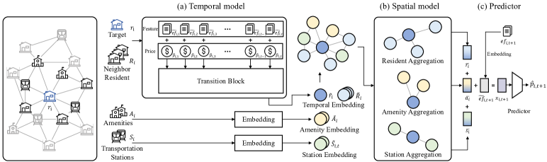
Figure 1. The overall architecture of ST-RAP consists of 3 different models: (a) temporal; (b) spatial, and (c) prediction models.

2. Related Work

The existing literature on data-driven real estate appraisal largely falls into two categories: (1) traditional automated valuation models (AVMs) and (2) recent graph-based models. Traditional AVMs focus on property features such as size, age, and location, and employ simple ML models such as linear regression (Şipoş et al., 2008; Ahn et al., 2012), support vector machines (Smola and Schölkopf, 2004; Lin and Chen, 2011), and neural networks (Peterson and Flanagan, 2009; Law et al., 2019; Poursaeed et al., 2018; Wang et al., 2021; Chanasit et al., 2021). Compared to methods that rely on domain expertise (Baum et al., 2017; Guo et al., 2014; Gonzalez and Laureano-Ortiz, 1992; Betts and Ely, 2020; Shiller and Weiss, 1999), AVMs are efficient and scalable, improving their performance as more data becomes available. Despite their advantages, they struggle to capture the spatial relationships between real estate transactions, which can significantly enhance real estate appraisal.

To address this, recent studies have utilized graph neural networks (GNN) to model spatial relationships between properties (Bin et al., 2019; Zhang et al., 2021; Li et al., 2022; Xiao et al., 2023a; Xiao et al., 2023b). MugRep (Zhang et al., 2021) constructs multiple graphs to capture the relationships between individual transactions and residential communities (Veličković et al., 2018). ReGram (Li et al., 2022) further employs an attention module to account for regional differences.

Despite these advancements, prior GNN-based methods face challenges in capturing the temporal trends (e.g., price inflation) in real estate values. They attempt to integrate temporal trends by incorporating features such as mean and variance of past transaction values as additional inputs. Nevertheless, such an approach is insufficient for fully capturing the complex, dynamic temporal pattern of real estate values. Furthermore, these models fail to sufficiently leverage amenities and transportation data, which are critical factors in real estate appraisal.

In response, we introduce ST-RAP, a spatiotemporal framework for real estate appraisal. ST-RAP not only captures temporal dynamics but also includes a heterogeneous GNN to encapsulate the relationships between transactions, and local amenities.

3. Preliminaries

3.1. Dataset

We construct a real estate dataset from the Republic of Korea (2016-2020), which is categorized into four categories: Transaction, Resident, Amenity, and Transportation, as shown in Table 1. We generate connections between entities where the entities within a 5-kilometer radius are considered to be connected.

Table 1. Statistics of real estate dataset.

Category	# of events	# of features	# of connections to Resident
Transaction	3,632,022	13	-
Resident	41,871	25	3,449,406
Amenity	14,851	10	562,521
Transportation	13,549	7	1,412,919

The Transaction category contains 3.6 million records, each defined by 13 attributes including transaction type, date, land area, and price. The Resident category is composed of 25 features (e.g., location, number of buildings, and the year of construction), with a total of 41,871 records. Each resident is connected based on geographical proximity (total 3.4 million edges). Additionally, our dataset comprises 15,000 amenities (schools, hospitals, and department stores) and 13,500 transportation stations (train, subway, and bus), generating 1.9 million connections to the residents.

In contrast to previous studies using 0.3 million transactions, our dataset contains 3.6 million transactions that are planned to be publicized. We believe that our dataset will serve as a valuable resource to promote research in real estate appraisal.

3.2. Problem Formation

We represent a residential community as $r_{i}$, where $1\leq i\leq N_{r}$, with $N_{r}$ being the total number of residents in the dataset. A transaction event within resident $r_{i}$ is defined as $e_{i,t}$, with $1\leq t\leq T_{i}$ and $T_{i}$ denotes the total number of transaction events within resident $r_{i}$.

Each transaction event, $e_{i,t}$, is described by a feature vector $ef_{i,t}\in\mathbb{R}^{d_{e}}$ and its price $p_{i,t}\in\mathbb{R}$, with $d_{e}$ representing the dimension of the transaction feature. Hence, we express $e_{i,t}$ as

(1) $$e_{i,t}=\{ef_{i,t},p_{i,t}\}.$$

For each residential community $r_{i}$, we define a resident feature vector as $rf_{i}\in\mathbb{R}^{d_{r}}$ and a sequence of transaction events as $h_{i,1:T_{i}}$, where $d_{r}$ denotes the dimension of the resident feature. Resident $r_{i}$ is therefore represented as

(2) $$r_{i,1:T_{i}} =\{rf_{i},h_{i,1:T_{i}}\}$$

(3) $$h_{i,1:T_{i}} =[e_{i,1},e_{i,2},...,e_{i,T_{i}}].$$

In the sequence of transactions $h_{i,1:T_{i}}$, $e_{i,T_{i}}$ refers to the latest transaction, while $e_{i,1}$ refers to the earliest transaction in $r_{i}$.

Residents are connected based on geographical proximity, and we define the set of connected residents to $r_{i}$ as:

(4) $$R_{i}=\{r_{v}\;|\;r_{v}\text{ is connected to }r_{i}\}.$$

Resident $r_{i}$ is also connected to nearby amenities and transportation stations. Each amenity and station is represented as $a_{j}\in\mathbb{R}^{d_{a}}$ and $s_{j}\in\mathbb{R}^{d_{s}}$, respectively, where $d_{a}$ and $d_{s}$ denote the dimensions of the corresponding feature vectors. The sets of connected amenities and transportation stations to $r_{i}$ are defined as:

(5) $$A_{i}=\{a_{v}\;|\;a_{v}\text{ is connected to }r_{i}\}$$

(6) $$S_{i}=\{s_{v}\;|\;s_{v}\text{ is connected to }r_{i}\}.$$

Our goal is to predict the price $p_{i,t+1}$ of the next transaction event $e_{i,t+1}$, given the transaction features $ef_{i,t+1}$. We seek to incorporate spatiotemporal factors by utilizing the history of past transaction events $r_{i,1:t}$ and connected entities, including residents $R_{i}$, amenities $A_{i}$, and transportation stations $S_{i}$.

We train a function $f$ parameterized by $\theta$ to perform prediction:

(7) $$\hat{p}_{i,t+1}=f_{\theta}(ef_{i,t+1},r_{i,1:t},R_{i},A_{i},S_{i}).$$

4. Method

This section presents ST-RAP, a hierarchical architecture with temporal and spatial models. The temporal model captures the temporal trend of transaction prices based on transaction history. Afterward, the spatial model aggregates the output of the temporal model with nearby entities. The overall architecture is illustrated in Figure 1.

4.1. Temporal model

Here, we describe the temporal model as illustrated in Figure.1(a).

Embedding. For each transaction event $e_{i,t}$, we linearly embed the price and feature ($p_{i,t}$, $ef_{i,t}$) as $\tilde{p_{i,t}}\in\mathbb{R}^{d_{h}}$ and $\tilde{ef_{i,t}}\in\mathbb{R}^{d_{h}}$, where $d_{h}$ is a hidden dimension of the embedding matrix. Then, we obtain the transaction embedding, $\tilde{e}_{i,t}$, by summing up these vectors as

(8) $$\tilde{e}_{i,t}=\tilde{p}_{i,t}+\tilde{ef}_{i,t}.$$

Subsequently, for each transaction history $h_{i,1:t}$, the transaction history embedding $\tilde{h}_{i,1:t}$ is denoted as

(9) $$\tilde{h}_{i,1:t}=[\tilde{e}_{i,1},\tilde{e}_{i,2},...,\tilde{e}_{i,t}].$$

Temporal modelling. After the embedding stage, the transaction history matrix, $\tilde{h}_{i,1:t}$, is processed by a transition model to effectively capture the temporal dynamics of the transaction events. Here, we employ a Gated Recurrent Unit (GRU (Chung et al., 2014)) as the transition model. The output of GRU is defined as

(10) $$\tilde{h}^{\prime}_{i,1:t}=GRU(\tilde{h}_{i,1:t}).$$

By adding the linearly embedded resident feature, $\tilde{rf}_{i}\in\mathbb{R}^{d_{h}}$, to the last sequence of the GRU-processed history embedding, $\tilde{h}^{\prime}_{i,t}$, we derive the resident embedding that reflects temporal information.

(11) $$\tilde{r}_{i}=\tilde{h}^{\prime}_{i,t}+\tilde{rf}_{i}.$$

4.2. Spatial model

Here, we describe the spatial model as demonstrated in Figure.1(b).

Embedding. As described in the equations 4, 5, 6, the resident $r_{i}$ is connected to the nearby residents $R_{i}$, amenities $A_{i}$, and transportations $S_{i}$. Each resident $r_{v}\in R_{i}$ is embedded by a temporal model as $\tilde{r}_{v}\in\mathbb{R}^{d_{h}}$. Then, each amenity $a_{v}\in A_{i}$ and transportation station in $s_{v}\in S_{i}$ are linearly embedded as $\tilde{a}_{v}\in\mathbb{R}^{d_{h}}$ and $\tilde{s}_{v}\in\mathbb{R}^{d_{h}}$.

Spatial modelling. After embedding, we aggregate the features of nearby residents, amenities, and transportation stations to capture the diverse spatial relationships between these entities. Given the heterogeneity of the entity types, we utilize a Heterogeneous Graph Neural Network (HGNN (Zhang et al., 2019)) to construct a comprehensive representation of spatial features.

Given the resident vector $\tilde{r}_{i}$ and its neighbor entities $\tilde{R}_{i},\tilde{A}_{i}$, and $\tilde{S}_{i}$, the HGNN is constructed as:

(12) $$\bar{r}_{i} =W_{rr}(\sigma(W_{rv}\tilde{r}_{i}+W_{vr}\cdot\text{mean}_{\tilde{r}_{v}\in\tilde{R}_{i}}\tilde{r}_{v}))+b_{rr}$$

(13) $$\bar{a}_{i} =W_{ar}(\sigma(W_{av}\tilde{r}_{i}+W_{va}\cdot\text{mean}_{\tilde{a}_{v}\in\tilde{A}_{i}}\tilde{a}_{v}))+b_{ar}$$

(14) $$\bar{s}_{i} =W_{sr}(\sigma(W_{sv}\tilde{r}_{i}+W_{vs}\cdot\text{mean}_{\tilde{s}_{v}\in\tilde{S}_{i}}\tilde{s}_{v}))+b_{sr}$$

where $\sigma$ denotes the ReLU activation function. The shape of all weight matrices and bias vectors are identical to $W\in\mathbb{R}^{d_{h}\times d_{h}}$ and $b\in\mathbb{R}^{d_{h}}$. Here, the output is defined as $\bar{r}_{i}\in\mathbb{R}^{d_{h}},\bar{a}_{i}\in\mathbb{R}^{d_{h}},\bar{s}_{i}\in\mathbb{R}^{d_{h}}$.

Prediction. Finally, to predict the price of the transaction event $e_{i,{t+1}}$, we construct the state $x_{i,t+1}$ by aggregating the transaction embedding $\tilde{ef}_{i,t+1}$ with the spatiotemporal features $\bar{r}_{i},\bar{a}_{i},\bar{s}_{i}$ as

(15) $${x}_{i,t+1}=\tilde{ef}_{i,t+1}+\bar{r}_{i}+\bar{a}_{i}+\bar{s}_{i}.$$

Then, we predict the price using a feed-forward network as

(16) $$\hat{p}_{i,t+1}=W_{hp}(\sigma(W_{xh}x_{i,{t+1}}+b_{xh}))+b_{hp}$$

where $\sigma$ denotes the ReLU activation, $W_{xh}\in\mathbb{R}^{d_{h}\times d_{h}},W_{hp}\in\mathbb{R}^{d_{h}\times 1}$ are weight matrices, and $b_{xh}\in\mathbb{R}^{d_{h}},b_{hp}\in\mathbb{R}$ are bias terms.

Training objective. The training objective is to minimize the mean absolute error (MAE) between the predicted price $\hat{p}_{i,t}$, and the actual price $p_{i,t}$. We define the loss function $\mathcal{L}$ as the average error across all residents and all transaction events, written as

(17) $$\mathcal{L}=\frac{1}{N_{r}T_{i}}\sum_{i=1}^{N_{r}}\sum_{t=1}^{T_{i}}|p_{i,t}-\hat{p}_{i,t}|.$$

By optimizing this objective, the model learns to make accurate predictions given the real estate dataset.

5. Experiments

5.1. Experimental Setup

We split the dataset into training, validation, and test sets in chronological order with a ratio of 90:5:5. We trained the model in the training set for 10 epochs, and used the validation set to select the best models. We use Mean Absolute Error (MAE), Root Mean Squared Error (RMSE), and Mean Absolute Percentage Error (MAPE) for evaluation. For MAE and RMSE, the unit price is 1,000,000 KRW. For all the metrics, the lower score indicates a better performance.

Baselines. We consider the following baselines: (i) two classical machine learning (ML) baselines (Linear Regression and Support Vector Regression) (Pedregosa et al., 2011), (ii) a rule-based model Repeat which simply outputs the previous transaction price in the same residential community, (iii) three graph-based models (GCN (Kipf and Welling, 2017), MugRep (Zhang et al., 2021) and ReGram (Li et al., 2022)) which captures the spatial dependency between real estate transactions and residential communities.

Implementation Details. For all the methods, we tuned the hyperparameters using the k-fold cross-validation $(K=5)$. We used the AdamW (Loshchilov and Hutter, 2017) with varying learning rates of $\{0.1,0.01,0.001\}$ and $L_{2}$ weight regularization strength from $\{0.01,0.001,0.0001\}$. We set the batch size to 128, weight decay to 1e-5, and gradient clipping to 0.5 and trained for 100 epochs. For MugRep and ReGram, we search the number of attention heads from {1,2,4,8}.

Table 2. Performance comparison for real estate appraisal. The results are averaged over 5 random seeds.

Method	MAE (M) $\downarrow$	RMSE (M) $\downarrow$	MAPE $\downarrow$
LR	105.09 $\pm$1.52	194.59 $\pm$1.18	65.62% $\pm$1.05%
SVR	90.31 $\pm$3.30	137.96 $\pm$1.99	53.22% $\pm$2.21%
Repeat	46.01 $\pm$0.00	97.55 $\pm$0.00	28.67% $\pm$0.00%
GCN (Kipf and Welling, 2017)	50.17 $\pm$2.19	94.13 $\pm$3.45	30.87% $\pm$0.02%
MugRep (Zhang et al., 2021)	35.46 $\pm$2.43	74.08 $\pm$3.64	22.29% $\pm$0.01%
ReGram (Li et al., 2022)	34.61 $\pm$4.61	64.48 $\pm$5.03	21.81% $\pm$0.03%
ST-RAP	21.77 $\pm$0.78	48.03 $\pm$1.70	13.72% $\pm$0.05%

5.2. Main Results

Table 2 provides the comparative analysis. Comparing regression models (LR, SVR) to the rule-based model (Repeat), Repeat significantly outperformed regression models. Repeat can be seen as the simplest version of a temporal model, as it outputs the price of the most recent transaction within a residential community. This notable gap implies that the integration of temporal information is crucial in accurately appraising real estate prices.

In addition, we observed that GNN-based models (GCN, MugRep, and Regram), outperform non-spatial models (LR and SVR) across all the evaluation metrics. These findings emphasize the significance of incorporating spatial information for real estate appraisal.

Most importantly, our proposed model, ST-RAP, demonstrates a remarkable improvement over all the comparative models. ST-RAP integrates both temporal and spatial dependencies among residents, amenities, and transportation stations. This improvement affirms the effectiveness of reflecting spatiotemporal factors and the use of heterogeneous graphs for an accurate real estate appraisal.

5.3. Ablation Studies

Architecture. We conducted an architecture ablation study by separating the spatial (S-RAP) and temporal (T-RAP) components of ST-RAP. The transactions are classified into three groups for this analysis: ALL, which includes all transactions, the COLD group, representing transactions without any historical records within the residents, and the WARM group, representing the remaining transactions with historical records.

Table 3. MAE of S-RAP, T-RAP, and ST-RAP for all transactions (ALL), transactions without any historical records within residents (COLD), and the others (WARM).

Mod	ALL $\downarrow$	COLD $\downarrow$	WARM $\downarrow$
S-RAP	26.98 $\pm$0.39	212.20 $\pm$36.86	26.23 $\pm$0.37
T-RAP	22.62 $\pm$0.54	230.52 $\pm$12.22	21.99 $\pm$0.54
ST-RAP	21.77 $\pm$0.78	189.42 $\pm$12.68	21.21 $\pm$0.76

Table 3 shows that ST-RAP outperforms both S-RAP and T-RAP across all metrics, emphasizing the importance of integrating both temporal trends and spatial factors in the model.

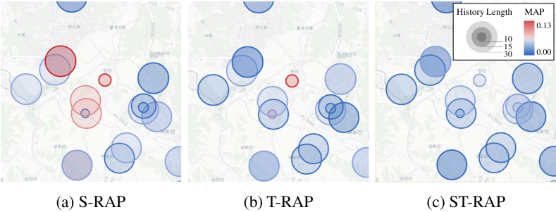
Figure 2. Error distribution of S-RAP, T-RAP, and ST-RAP. The diameter indicates the number of transaction histories.

ST-RAP’s improved performance over S-RAP underscores the importance of temporal dynamics. In contrast, the sharp performance drop for T-RAP in the COLD group highlights the importance of spatial modeling when temporal data is scarce. This is further illustrated in Figure 2, where S-RAP fails to provide accurate predictions even with an abundance of historical transaction records, and T-RAP’s performance diminishes in the absence of such records.

These results reiterate the necessity of incorporating both spatial and temporal aspects for precise real estate appraisal.

Table 4. Ablation of the maximum history length.

History Len	1	2	5	10	20	30	50
MAE (M)	26.98	24.73	22.59	22.24	21.93	21.77	21.89

History Length. To evaluate the importance of temporal information on transaction value prediction, we conduct an ablation study varying the sequence length (i.e., the number of previous transactions in the residential community). Table 4 displays the performance based on the sequence length for GRU. For both ST-RAP and T-RAP, which consider temporal information, performance improves as the sequence length increases.

Table 5. Ablation of the temporal model.

Architecture	MAE (M) $\downarrow$	RMSE (M) $\downarrow$	MAPE $\downarrow$
Transformer	24.35 $\pm$0.71	54.73 $\pm$0.43	15.32% $\pm$0.44%
GRU	21.77 $\pm$0.78	48.03 $\pm$1.70	13.72% $\pm$0.05%

Temporal Model. While transformer-based models have shown impressive capabilities in handling unstructured time-series data such as language, their performance has been found to be suboptimal when applied to structured time-series data  (Xu et al., 2020; Cirstea et al., 2022; Li et al., 2019; Zhou et al., 2021; Wen et al., 2023; Wu et al., 2021; Zeng et al., 2022). Replacing our GRU-based temporal model with a transformer led to a drop in performance, as depicted in Table 5. This observation underscores the need for an inductive bias that transformers may lack when dealing with structured temporal trends.

6. Conclusion

We introduced ST-RAP, a novel spatial-temporal framework for real estate appraisal. By integrating the temporal dynamics via a recurrent model and spatial relationships through a heterogeneous graph model, ST-RAP significantly outperforms previous baselines which underscore the importance of reflecting the spatiotemporal factors in real estate appraisal. In addition, we plan to publicize both our code and dataset to foster future research in this field.

7. Acknowledgements

This work was supported by Woomi Construction Co. Ltd. (G01210242), Institute for Information & communications Technology Planning & Evaluation(IITP) grant funded by the Korea government(MSIT) (No. 2020-0-00368, A Neural-Symbolic Model for Knowledge Acquisition and Inference Techniques), and the National Research Foundation of Korea (NRF) grant funded by the Korea government (MSIT) (No. NRF-2022R1A2B5B02001913).

References

- (1)
- Ahn et al. (2012) Jae Joon Ahn, Hyun Woo Byun, Kyong Joo Oh, and Tae Yoon Kim. 2012. Using ridge regression with genetic algorithm to enhance real estate appraisal forecasting. Expert Systems with Applications 39, 9 (2012), 8369–8379.
- Baum et al. (2017) Andrew Baum, David Mackmin, and Nick Nunnington. 2017. The Income Approach to Property Valuation (7th. ed.). Routledge.
- Betts and Ely (2020) R Betts and Silas Ely. 2020. Basic Real Estate Appraisal (5th. ed.). South-Western.
- Bin et al. (2019) Junchi Bin, Bryan Gardiner, Eric Li, and Zheng Liu. 2019. Peer-dependence valuation model for real estate appraisal. Data-Enabled Discovery and Applications 3 (2019), 1–11.
- Chanasit et al. (2021) Kankawee Chanasit, Ekapol Chuangsuwanich, Atiwong Suchato, and Proadpran Punyabukkana. 2021. A real estate valuation model using boosted feature selection. IEEE Access 9 (2021), 86938–86953.
- Chung et al. (2014) Junyoung Chung, Caglar Gulcehre, KyungHyun Cho, and Yoshua Bengio. 2014. Empirical evaluation of gated recurrent neural networks on sequence modeling. arXiv preprint arXiv:1412.3555 (2014).
- Cirstea et al. (2022) Razvan-Gabriel Cirstea, Chenjuan Guo, Bin Yang, Tung Kieu, Xuanyi Dong, and Shirui Pan. 2022. Triformer: Triangular, Variable-Specific Attentions for Long Sequence Multivariate Time Series Forecasting–Full Version. Proc. the International Joint Conference on Artificial Intelligence (IJCAI) (2022).
- Demyanyk and Van Hemert (2011) Yuliya Demyanyk and Otto Van Hemert. 2011. Understanding the subprime mortgage crisis. The review of financial studies 24, 6 (2011), 1848–1880.
- Gonzalez and Laureano-Ortiz (1992) Avelino J. Gonzalez and Raymond Laureano-Ortiz. 1992. A case-based reasoning approach to real estate property appraisal. Expert Systems with Applications 4, 2 (1992), 229–246.
- Guo et al. (2014) Jingjuan Guo, Shoubo Xu, and Zhuming Bi. 2014. An integrated cost-based approach for real estate appraisals. Information Technology and Management 15 (2014), 131–139.
- Kipf and Welling (2017) Thomas N. Kipf and Max Welling. 2017. Semi-Supervised Classification with Graph Convolutional Networks. Proc. the International Conference on Learning Representations (ICLR) (2017).
- Law et al. (2019) Stephen Law, Brooks Paige, and Chris Russell. 2019. Take a look around: using street view and satellite images to estimate house prices. ACM Transactions on Intelligent Systems and Technology (TIST) 10, 5 (2019), 1–19.
- Lee et al. (2022) Hojoon Lee, Dongyoon Hwang, Hyunseung Kim, Byungkun Lee, and Jaegul Choo. 2022. Draftrec: personalized draft recommendation for winning in multi-player online battle arena games. In Proceedings of the ACM Web Conference 2022. 3428–3439.
- Li et al. (2022) Chih-Chia Li, Wei-Yao Wang, Wei-Wei Du, and Wen-Chih Peng. 2022. Look Around! A Neighbor Relation Graph Learning Framework for Real Estate Appraisal. Proc. the AAAI Conference on Artificial Intelligence (AAAI) (2022).
- Li et al. (2019) Shiyang Li, Xiaoyong Jin, Yao Xuan, Xiyou Zhou, Wenhu Chen, Yu-Xiang Wang, and Xifeng Yan. 2019. Enhancing the Locality and Breaking the Memory Bottleneck of Transformer on Time Series Forecasting.
- Lin and Chen (2011) Hongyu Lin and Kuentai Chen. 2011. Predicting price of Taiwan real estates by neural networks and support vector regression. In Proc. of the 15th WSEAS Int. Conf. on Syst. 220–225.
- Loshchilov and Hutter (2017) Ilya Loshchilov and Frank Hutter. 2017. Decoupled weight decay regularization. arXiv preprint arXiv:1711.05101 (2017).
- Pagourtzi et al. (2003) Elli Pagourtzi, Vassilis Assimakopoulos, Thomas Hatzichristos, and Nick French. 2003. Real estate appraisal: a review of valuation methods. Journal of property investment & finance 21, 4 (2003), 383–401.
- Pavlov and Wachter (2011) Andrey Pavlov and Susan Wachter. 2011. Subprime lending and real estate prices. Real Estate Economics 39, 1 (2011), 1–17.
- Pedregosa et al. (2011) Fabian Pedregosa, Gaël Varoquaux, Alexandre Gramfort, Vincent Michel, Bertrand Thirion, Olivier Grisel, Mathieu Blondel, Peter Prettenhofer, Ron Weiss, Vincent Dubourg, Jake VanderPlas, Alexandre Passos, David Cournapeau, Matthieu Brucher, Matthieu Perrot, and Edouard Duchesnay. 2011. Scikit-learn: Machine Learning in Python. Journal of Machine Learning Research 12 (2011).
- Peterson and Flanagan (2009) Steven Peterson and Albert Flanagan. 2009. Neural network hedonic pricing models in mass real estate appraisal. Journal of real estate research 31, 2 (2009), 147–164.
- Poursaeed et al. (2018) Omid Poursaeed, Tomáš Matera, and Serge Belongie. 2018. Vision-based real estate price estimation. Machine Vision and Applications 29, 4 (2018), 667–676.
- Shiller and Weiss (1999) Robert J. Shiller and Allan N. Weiss. 1999. Evaluating Real Estate Valuation Systems. The Journal of Real Estate Finance and Economics 18 (1999), 147–161.
- Şipoş et al. (2008) Ciprian Şipoş, Eng Adrian Crivii, and MBA FRICS. 2008. A linear regression model for real estate appraisal. In WAVO Valuation Congress Valuation in Diversified and Emerging Economies. 17–18.
- Smola and Schölkopf (2004) Alex J Smola and Bernhard Schölkopf. 2004. A tutorial on support vector regression. Statistics and computing 14 (2004), 199–222.
- Veličković et al. (2018) Petar Veličković, Guillem Cucurull, Arantxa Casanova, Adriana Romero, Pietro Liò, and Yoshua Bengio. 2018. Graph Attention Networks. Proc. the International Conference on Learning Representations (ICLR) (2018).
- Wang et al. (2021) Pei-Ying Wang, Chiao-Ting Chen, Jain-Wun Su, Ting-Yun Wang, and Szu-Hao Huang. 2021. Deep learning model for house price prediction using heterogeneous data analysis along with joint self-attention mechanism. IEEE Access 9 (2021), 55244–55259.
- Wen et al. (2023) Qingsong Wen, Tian Zhou, Chaoli Zhang, Weiqi Chen, Ziqing Ma, Junchi Yan, and Liang Sun. 2023. Transformers in Time Series: A Survey. Proc. the International Joint Conference on Artificial Intelligence (IJCAI) (2023).
- Wu et al. (2021) Haixu Wu, Jiehui Xu, Jianmin Wang, and Mingsheng Long. 2021. Autoformer: Decomposition Transformers with Auto-Correlation for Long-Term Series Forecasting. Proc. the Advances in Neural Information Processing Systems (NeurIPS).
- Xiao et al. (2023a) Congxi Xiao, Jingbo Zhou, Jizhou Huang, Tong Xu, and Hui Xiong. 2023a. Spatial Heterophily Aware Graph Neural Networks. arXiv preprint arXiv:2306.12139 (2023).
- Xiao et al. (2023b) Congxi Xiao, Jingbo Zhou, Jizhou Huang, Hengshu Zhu, Tong Xu, Dejing Dou, and Hui Xiong. 2023b. A contextual master-slave framework on urban region graph for urban village detection. In 2023 IEEE 39th International Conference on Data Engineering (ICDE). IEEE, 736–748.
- Xu et al. (2020) Mingxing Xu, Wenrui Dai, Chunmiao Liu, Xing Gao, Weiyao Lin, Guo-Jun Qi, and Hongkai Xiong. 2020. Spatial-temporal transformer networks for traffic flow forecasting. arXiv preprint arXiv:2001.02908 (2020).
- Zeng et al. (2022) Ailing Zeng, Muxi Chen, Lei Zhang, and Qiang Xu. 2022. Are Transformers Effective for Time Series Forecasting? Proc. the AAAI Conference on Artificial Intelligence (AAAI).
- Zhang et al. (2019) Chuxu Zhang, Dongjin Song, Chao Huang, Ananthram Swami, and Nitesh V Chawla. 2019. Heterogeneous graph neural network. In Proc. the ACM SIGKDD International Conference on Knowledge Discovery and Data Mining (KDD). 793–803.
- Zhang et al. (2021) Weijia Zhang, Hao Liu, Lijun Zha, Hengshu Zhu, Ji Liu, Dejing Dou, and Hui Xiong. 2021. MugRep: A multi-task hierarchical graph representation learning framework for real estate appraisal. In Proc. the ACM SIGKDD International Conference on Knowledge Discovery and Data Mining (KDD). 3937–3947.
- Zhou et al. (2021) Haoyi Zhou, Shanghang Zhang, Jieqi Peng, Shuai Zhang, Jianxin Li, Hui Xiong, and Wancai Zhang. 2021. Informer: Beyond Efficient Transformer for Long Sequence Time-Series Forecasting. Proc. the AAAI Conference on Artificial Intelligence (AAAI) (2021).