Analyzing Complex Systems with Cascades Using Continuous-Time Bayesian Networks

Abstract

Interacting systems of events may exhibit cascading behavior where events tend to be temporally clustered. While the cascades themselves may be obvious from the data, it is important to understand which states of the system trigger them. For this purpose, we propose a modeling framework based on continuous-time Bayesian networks (CTBNs) to analyze cascading behavior in complex systems. This framework allows us to describe how events propagate through the system and to identify likely sentry states, that is, system states that may lead to imminent cascading behavior. Moreover, CTBNs have a simple graphical representation and provide interpretable outputs, both of which are important when communicating with domain experts. We also develop new methods for knowledge extraction from CTBNs and we apply the proposed methodology to a data set of alarms in a large industrial system.

1 Introduction

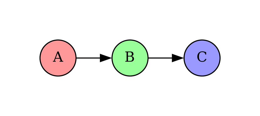
(a) CTBN graph $\mathcal{G}$

(b) State space graph $\mathcal{G}_{s}$

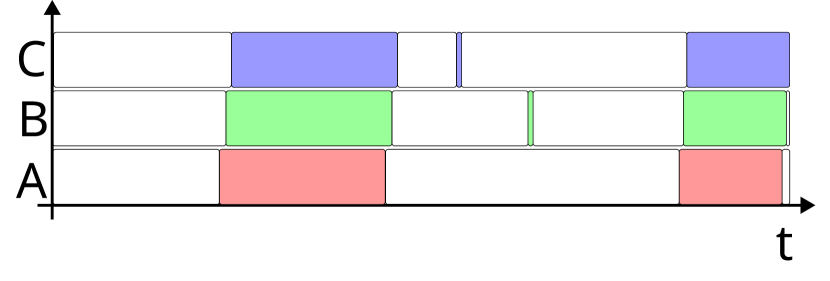
(c) Trajectory

Figure 1: a) Graph $\mathcal{G}$ of a CTBN consisting of three nodes ($A$, $B$, $C$). b) State space graph $\mathcal{G}_{s}$ of the CTBN, i.e., nodes represent states of the CTBN and two states are adjacent if a transition from one to the other, and vice versa, is possible. c) A trajectory for the CTBN. A white segment indicates that the corresponding process is in state 0 (off), while a colored segment indicates that the corresponding process is in state 1 (on).

Many real-world phenomena can be modeled as interacting sequences of events of different types. This includes social networks where user activity influences the activity of other users [11]. In healthcare, patient history may be modeled as a sequence of events [46]. In this paper, we focus on an industrial application in which the events are alarm signals of a complex engineered system. As an illustration, consider Figure 1. Three different alarms ($A$, $B$, and $C$) monitor a process each within an industrial system. These processes may, for instance, represent measured temperatures or pressures. An alarm transitions to on when its the process it monitors leaves a prespecified range of values and transitions to off when the process is again within the range corresponding to ‘normal operation’. In Figure 1(c), the colored segments correspond to the alarm being on. When an alarm changes state, we say that an event occurs.

In particular, we are interested in systems that exhibit a cascading behavior in the sense that events are strongly clustered in time. Therefore, we should use a model class which is capable of expressing cascades. However, important information may also be contained in non-cascading parts of the observed data. This is explained by the fact that our goal is twofold: We wish to understand which states of the system lead to cascades, and we also wish to understand how different components of the system interact. These goals are connected as understanding the inner workings of the system will also help us understand the cascading behavior. We can achieve both by using continuous-time Bayesian networks (CTBNs) [32], a class of parsimonious Markov processes with a discrete state space. Moreover, CTBNs are equipped with a graphical representation of how different components interact. In our application, data is sampled at a very high frequency and using a continuous-time modeling framework makes for a conceptually and computationally simple approach. In CTBNs, we define the concept of a sentry state which is a state that may lead to an imminent cascade. In an industrial setting, identifying such states may give operators an early warning, which in turn facilitates the mitigation of underlying issues before an actual alarm cascade occurs. Moreover, sentry states can be used to apply state-based alarm techniques [18], which otherwise require a known alarm structure.

In applications to complex systems, analysts often need to communicate findings to domain experts. CTBNs also allow easy communication using their graphical representation which is crucial for their applicability to real-world problems. We describe a useful interpretation of the graph of a CTBN and provide some new results in this direction. We apply the methods developed in this paper to a challenging data set from the European Spallation Source (ESS), a research facility in Lund, Sweden. This data set describes how alarms propagate through a subsystem of the neutron source at ESS.

The paper is structured as follows. We start with a description of the ESS data as this motivates the following developments (Section 2). In Section 3, we describe related work and compare CTBNs with other approaches. Section 4 describes continuous-time Bayesian networks. Sections 5 and 6 contain the main theoretical contributions of the paper: Section 5 describes the concept of a sentry state while Section 6 explains how the graphical representation of a CTBN may assist interpretation and communication. Section 7 presents numerical experiments, including a description of the ESS data analysis. A discussion concludes the main paper and the appendices contain auxiliary results.

2 Data Set

The European Spallation Source ERIC (ESS) is a large research facility which is being built in Lund, Sweden. Its main components include a linear proton accelerator, a tungsten target, and a collection of neutron instruments [16]. It comprises a large number of systems, including an integrated control system [15]. The facility has a goal of 95% availability and state-of-the-art alarm handling may contribute to reaching this goal.

Operators of large facilities are often facing large quantities of data in real time and good tools may helpsystem understanding and support decision making. Operators rely on alarm systems to warn them about unexpected behavior. However, alarm problems are common [18]. One example is that of cascading alarms. In large facilities, different alarms monitor different processes and when an issue occurs this may result in a large number of alarms that occur within a short time frame due to the interconnectedness of the different processes. Operators will often find it difficult to respond to such cascades as hundreds or thousands of alarms may sound, making it difficult to identify the underlying issue.

The alarm system has two purposes. One, it should help operators foresee and mitigate fault situations. Two, it should help operators understand a fault situation. In this paper, we illustrate how the methods we propose can help achieve these goals using data from the accelerator cryogenics plant at ESS, which has been in operation since 2019.

Example 1 (Simplified ESS alarm network).

In this example, we will look at a simplified version of the alarm system at ESS. Each of the alarm processes P1, T1, P2, T2, P3, T3, S1, S2, S3, and S4 in Figure 2 (left) monitors a physical process, e.g., a temperature or a pressure. At each time point, each alarm process is either 1 (alarm is on) or 0 (alarm is off). An edge, $\rightarrow$, in the graph implies a dependence in transition rates, e.g., the rate with which P1 changes its state depends only on the current states of P1, T1, and S4. Alarm cascades occur when a certain state triggers a fast progression of alarm onsets. In this formalism, this is modeled by the dependence of transition rates on the current state: therefore, cascades tend to unfold along the directed edges of the graph.

Large engineered systems can often be divided into subsystems (in Figure 2, Systems 1, 2, 3, and 4). In alarm networks, a group of alarms may monitor processes that are known to be correlated as they are measured from the same subsystem. Moreover, many systems of a realistic size comprise so many alarms or variables that processes must be grouped into subsystems to enable a system-level understanding of their dependencies. In Section 6, we show that graphical representations using these subsystems (e.g., Figure 2 (right)), instead of the processes themselves, are also useful and have a clear interpretation.

Figure 2: Graphs from Example 2. Left: Graph such that each node represents an alarm process. Edges, $\rightarrow$, represent sparsity in transition rate dependence. The transition rate of each process, $A$, only depends on its own state and the states of its parent processes, i.e., processes $B$ such that the edge $B\rightarrow A$ is in the graph. Right: Graph representing transition rate dependencies between entire subsystems rather than between individual alarm processes. This graph is computed from the larger graph on the left and can be given a mathematical interpretation (Section 6).

 

3 Related Work

Our work has connections to several major directions in the literature of dynamical models. We will focus on methods that are relevant for modeling cascades of events.

Continuous-time Markov processes with a discrete state space are often used as models of cascading failures in complex networks such as power grids [34, 28] and as models of burst behavior in biological cells [6]. They are also used in chemistry [4], reliability modeling [20], queueing theory [26], and genetics [7]. Graphs may be used as representations of networks and several methods use graphs to represent cascading structures [30, 29]. Some of these methods use simple models of contagion and study influential nodes in a graph [22]. Among these we find the independent cascade model and the linear threshold model [21, 12]. These models are targeted at applications in which cascades or ‘epidemics’ are the salient feature.

Change-point detection methods aim to recover the time points at which distributional changes occur. There is a large literature on change-point detection in various classes of stochastic processes and application fields such as neuroscience [37], DNA sequence segmentation [9], speech recognition [39], and climate change [36]. [3] provides a survey on change-point methods in discrete-time models. [42] also provides a survey and discusses subsampling of continuous-time processes. [45] provides a method for change-point detection in a class of multivariate point processes. There are subtle, but important, differences between the task at hand and change-point detection. The alarm network that motivates our work is thought to operate in the same mode throughout the observation period. Moreover, the detection of cascades is trivial in this application as they are evident from simply visualizing the data. Instead, we focus on identifying the states that are likely to lead to a cascade. In addition, our modeling approach should allow for a qualitative understanding of the interactions between system components.

As a result, we would like to explicitly model how events propagate through the system. A traditional approach is to use point processes [13]. In our setting, we can think of a point process as a sequence of pairs $(t_{1},e_{1}),(t_{2},e_{2}),(t_{3},e_{3}),\ldots$ such that $(t_{i})$ is an increasing sequence of time points and $(e_{i})$ denotes the type of event. Point process models have been used for modeling cascades of failures [23]. [35] describes self-exciting point processes that model cascading behavior using explicit exogenous influences on the system. These methods can in principle also be applied in the setting of this paper. The CTBN-based method proposed in this paper models the state of the system directly and this facilitates the notion of sentry states which is central to this paper. Moreover, as the alarm status takes values in a discrete set, the CTBN provides a natural representation of the alarm data.

While the above describes general approaches to the modeling of dynamical systems with cascading behavior, there are also more specialized methods for handling or analyzing alarm cascades in large industrial systems. We now summarize the connections to this work; see also [2], which is a recent review of methods for alarm cascade problems (in that paper known as alarm floods). In short, so-called knowledge-based methods use expert knowledge of the cause-effect relations in the system to find root causes and explain alarm cascades. Among these are multilevel flow modeling [24] and signed directed graphs [44]. In contrast, there is also a large number of data-based methods. Data-based methods can be subdivided into classes of methods depending on their purpose. Some approaches aim to classify the fault type from an input sequence of alarms or to simply reduce the number of alarms, e.g., using data mining, clustering, or machine learning methods such as artificial neural networks [47, 38, 5]. This goal is somewhat different from ours and our method is more closely related to methods using probabilistic graphical models, in particular dynamic Bayesian networks [19]. These methods produce an easily interpretable output represented by a graph. Our contribution in relation to this prior work is twofold. 1) We introduce the CTBN framework as a natural further development of alarm modeling. This allows continuous-time modeling which is useful for our data as it is collected using a very high sampling rate. Discretization of time will therefore either lead to a prohibitively large number of time intervals or to a loss of temporal information if using fewer, longer time intervals. 2) We define the novel concept of a sentry state which identifies a set of states that are of interest when analyzing cascading behavior. The sentry state concept may also be used in other alarm propagation models and is not specific to CTBNs.

4 Models

Continuous-time Bayesian networks (CTBNs; [31]) are a class of continuous-time Markov processes (CTMPs) with a factored state space and a certain sparsity in how transition rates depend on the current state. This sparsity can be represented by a directed graph. In this sense, they are similar to classical Bayesian networks [33] but their directed graphs are allowed to contain cycles. CTBNs have proved to be both effective and efficient representations of discrete-state continuous-time dynamical systems [1, 43, 25]. We first define a CTMP.

4.1 Continuous-Time Markov Processes

A continuous-time Markov process (CTMP) [41] is a continuous-time stochastic process $\mathbf{X}=\{X(t):t\in\left[0,\infty\right)\}$ which satisfies the following Markov property:

$$X(t_{1})\perp\!\!\!\perp X(t_{3})|X(t_{2}),\hskip 5.69046pt\forall\hskip 2.84544ptt_{1}<t_{2}<t_{3},$$ (1)

where $\cdot\perp\!\!\!\perp\cdot\mid\cdot$ denotes conditional independence. The state of the process $\mathbf{X}$ changes in continuous-time and takes values in the domain $S$ which we assume to be a finite set. In our application, each state $s\in S$ can be represented by an $n$-vector with binary entries indicating whether each alarm is on or off. A CTMP can be parameterized by the initial distribution $P_{0}$ and the intensity matrix $Q_{\mathbf{X}}$. The initial distribution $P_{0}$ is any distribution on the state space. The intensity matrix $Q_{\mathbf{X}}$ models the evolution of the stochastic process $\mathbf{X}$. Each row of $Q_{\mathbf{X}}$ sums to $0$ and models two distinct processes:

1. The time when $\mathbf{X}$ abandons the current state $x$, which follows an exponential distribution with parameter $q_{x}\in\mathbb{R}^{+}$.

2. The state to which $\mathbf{X}$ transitions when abandoning the state $x$. This follows a multinomial distribution with parameters $\theta_{xy}=\frac{q_{xy}}{q_{x}}$, $x,y\in S$, $x\neq y$.

An instance of the intensity matrix $Q_{X}$, when $S$ has three states, is as follows

$$Q_{\mathbf{X}}=\begin{bmatrix}-q_{x_{1}}&q_{x_{1}x_{2}}&q_{x_{1}x_{3}}\\ q_{x_{2}x_{1}}&-q_{x_{2}}&q_{x_{2}x_{3}}\\ q_{x_{3}x_{1}}&q_{x_{3}x_{2}}&-q_{x_{3}}\\ \end{bmatrix}\;\;\;\;q_{x_{i}}>0,q_{x_{i}{x_{j}}}\geq 0\;\forall\,i,j.$$ (2)

We say that a realization of a CTMP, $\sigma$, is a trajectory. This is a right-continuous, piecewise constant function of time. It can be represented as a sequence of time-indexed events,

$$\sigma=\{\langle t_{0},X(t_{0})\rangle,\langle t_{1},X(t_{1})\rangle,...,\langle t_{I},X(t_{I})\rangle\}, t_{0}<t_{1}<\dots<t_{I}.$$ (3)

4.2 Continuous-Time Bayesian Networks

General CTMPs do not assume any sparsity. CTBNs impose structure on a CTMP by assuming a factored state space $S=\{S_{1}\times S_{2}\times\dots\times S_{L}\}\;$ such that $X(t)=(X_{1}(t),\ldots,X_{L}(t))\in S$ where each $S_{j}$, $j=1,...,L$, represents the domain of a distinct component of the process. In the alarm data, $S_{j}=\{0,1\}$ for each $j$ and $X_{j}(t)$ indicates if the $j$’th alarm is on or off at time $t$. The structure imposed by the CTBN is useful when interpreting a learned model. In essence, the CTBN framework allows us to learn which components of the system act independently, or conditionally independently, and this can be communicated to experts.

A CTBN is a tuple ${\cal N}=\langle P_{0},\mathbf{X},{\cal G},{\bf Q}_{X}\rangle$ where $\mathbf{X}=\{\mathbf{X}_{1},\ldots,\mathbf{X}_{L}\}$ is a set of stochastic processes. A CTBN is specified by:

• An initial probability distribution $P_{0}$ on the factored state space $S$.

• A continuous-time transition model, specified as:

  • a directed (possibly cyclic) graph $\mathcal{G}$ with node set X;

  • a set of conditional intensity matrices $\mathbf{Q}_{\mathbf{X}_{j}|\text{Pa}(\mathbf{X}_{j})}$ for each process $\mathbf{X}_{j}\in\mathbf{X}$.

Given the graph $\mathcal{G}$, each node/process $\mathbf{X}_{j}$ has a parent set $\text{Pa}(\mathbf{X}_{j})$ consisting of all nodes/processes, $\mathbf{X}_{i}$, with an edge directed from $\mathbf{X}_{i}$ to $\mathbf{X}_{j}$ in $\mathcal{G}$, $\mathbf{X}_{i}\rightarrow\mathbf{X}_{j}$. A conditional intensity matrix (CIM) $\mathbf{Q}_{\mathbf{X}_{j}|\text{Pa}(\mathbf{X}_{j})}$ consists of a set of intensity matrices, one for each possible configuration of the states of the parent set $\text{Pa}(\mathbf{X}_{j})$ of the node/process $\mathbf{X}_{j}$, that is, one for each element of $\bigtimes_{\mathbf{X}_{i}\in\text{Pa}(\mathbf{X_{j}})}S_{i}$. The CIM describes how the transition intensity of process $j$ depends on the state of the system. However, it does not necessarily depend on the state of every other process, but only on the states of the processes that are parents of $j$.

In a CTBN only one process can transition at any given time. This assumption is reasonable for the alarm data as it is sampled at a high rate. When we apply this model to the alarm data, the interpretation is straightforward. The CIM of $\mathbf{X}_{j}$ describes how likely this alarm is to change its state (from on to off, or from off to on), and this only depends on the current state of the alarms in its parent set.

Example 2.

Assume we observe three alarm processes ($A$, $B$, and $C$) each monitoring a measured process and that we represent this by a stochastic process $\mathbf{X}$ that takes values in $\{0,1\}\times\{0,1\}\times\{0,1\}$ indicating the status of each of the three alarms. If $\mathbf{X}$ is a general CTMP, then the transition rates of each alarm process may depend on the entire state of the system. On the other hand, if $\mathbf{X}$ is a CTBN represented by the graph $\mathcal{G}$ in Figure 1(a) there is a certain sparsity in the way the transition rates depend on the current state. It follows directly that the transition rate of alarm process $C$ only depends on the states of processes $B$ and $C$. Similarly, the transition rate of alarm process $B$ only depends on the states of processes $A$ and $B$ while the transition rate of process $A$ only depends on its own state. When we learn a CTBN from data, we can therefore use its graph as a qualitative summary of the interconnections of the alarms. An edge from $A$ to $B$ in this graph means that a change in the state of $A$ may change the transition rates of $B$ and therefore cascades are expected to occur along the directed edges of the graph.

Another type of graphical representation is also useful: Figure 1(b) shows the associated factored state space graph $\mathcal{G}_{s}$. In this graph, each node represents a state (in contrast, in $\mathcal{G}$ each node represents a process/alarm) and edges represent the possible transitions between states. We will say that $\mathcal{G}$ is the graph of the CTBN and refer to $\mathcal{G}_{s}$ as the state space graph.

As we will see in the numerical experiments, CTBNs are capable of producing ‘cascading’ behavior. However, they also model the non-cascading behavior: This is important for our application because we would also like to use the information contained outside periods with cascades. The CTBN framework has the following advantages that are critical to our application: 1) It exploits the factorization of the multivariate alarm process to make it feasible to learn a CTBN model from data. 2) It takes into account the duration of an event as well as its occurrence. Moreover, it uses both the cascading and non-cascading data. 3) It has a graphical representation which is easy to interpret, thus facilitating communication.

4.3 Reward Function

A reward function is a function that maps the states of one or more processes onto a real number. We use a reward function to compute the discounted, expected number of transitions (that is, alarms changing their states) when starting the process in some initial state, $x$. A reward function consists of two quantities,

• $\mathcal{R}(x):S\rightarrow\mathbb{R}$, the instantaneous reward of state $X=x$, and

• $\mathcal{C}(x,x^{\prime}):S\times S\rightarrow\mathbb{R}$, the lump sum reward when $X$ transitions from state $x$ to state $x^{\prime}$.

We use the lump sum reward which is an indicator of transitions,

$$\mathcal{C}(x,x^{\prime})=1,\ \ \ \text{ for all }x,x^{\prime}\in S,$$ (4)

and we let the instantaneous reward be zero. We will use the infinite-horizon expected discounted reward [17],

$$V_{\alpha}(x)=\mathbb{E}_{x}\left[\sum_{i=0}^{\infty}e^{-\alpha t_{i+1}}C(X(t_{i}),X(t_{i+1}))+\int_{t_{i}}^{t_{i+1}}e^{-\alpha t}\mathcal{R}(X(t_{i}))dt\right]:t_{i}<t_{i+1}$$ (5)

where $\alpha>0$ is referred to as the discounting factor, $\mathbb{E}_{x}(\cdot)$ is the expectation when conditioning on $X(0)=x$, and the $t_{i}$’s are the transition times. We use $\mathcal{R}(x)=0$ for all $x$ and therefore

$$V_{\alpha}(x)={\mathbb{E}_{x}\left[\sum_{i=0}^{\infty}e^{-\alpha t_{i+1}}C(X(t_{i}),X(t_{i+1}))\right]}=\mathbb{E}\left[\sum_{i=0}^{\infty}e^{-\alpha t_{i+1}}\right]:t_{i}<t_{i+1}.$$ (6)

This simply counts the number of transitions including a discounting factor. Clearly, other reward functions can be chosen to analyze other or more specialized types of behavior. If, for instance, we are only interested in a subset of transitions we can modify the lump sum reward accordingly. A value of the parameter $\alpha$ can be chosen using, e.g., prior information on the length of typical cascades. This concludes the introduction of the modeling framework and the following sections describe the contributions of this paper.

5 Sentry State

Given a CTBN ${\cal N}=\langle P_{0},\mathbf{X},\mathcal{G},\mathbf{Q}_{X}\rangle$, we are interested in understanding its cascading behavior. We are in particular interested in identifying what we will call sentry states. A sentry state is a state which may trigger a ripple effect, that is, a sequence of fast transitions.

Example 3.

An example of a ripple effect can be found in the CTBN in Figure 1a which consists of three processes $\mathbf{X}_{A}$, $\mathbf{X}_{B}$ and $\mathbf{X}_{C}$, forming a chain $A\rightarrow B\rightarrow C$, and each taking values in $\{0,1\}$, $S_{A}=S_{B}=S_{C}=\{0,1\}$. The trajectory in Figure 1(c) shows that every time $A$ transitions, $B$ and $C$ quickly transition as well. In other words, when $A$ changes its state, a ripple effect occurs such that $B$ and $C$ also change states to match the state of their parent. The starting point of these cascades of events is a sentry state as defined in this section.

Figure 3: Visualization of Example 3: The state space graph (same graph as in Figure 1(b), but presented slightly differently) is annotated with EDNTs for each node (in parentheses) and a subset of nodes with relatively high EDNT values is highlighted. Sentry states are high EDNT states to which transitions from low EDNT states are possible and such a transition increases the risk of an imminent cascade. Some states with high EDNT tend to occur in the middle of a cascade which motivates using the REDNT metric. In this example, transitioning from $(A=0,B=0,C=0)$ to $(A=1,B=0,C=0)$ may trigger an alarm in $B$ which in turn may trigger an alarm in $C$, resulting in a cascade (note that only transitions along the edges in the state space graph are possible).

It is important to stress that we are interested in states that start a cascade of events. Intuitively, this means that we are assuming the existence of at least one state in the state space graph which is directly connected to the sentry state and which has a much smaller expected number of transitions than the sentry state itself. We can observe this in the example in Figure 1c: Before starting the sequence of transitions of processes $\mathbf{X}_{A}$, $\mathbf{X}_{B}$, and $\mathbf{X}_{C}$ from $0$ to $1$, the CTBN remained for a long time in state $\{A=0,B=0,C=0\}\in S$. Similarly, before changing the state of all processes $A$, $B$ and $C$ from $1$ to $0$, the CTBN remained for a long time in state $\{A=1,B=1,C=1\}\in S$.

5.1 Sentry State Identification

In order to identify a sentry state, we need to take a further step from the heuristic definition of a sentry state we have just given and formalize the concept. For this purpose, we first compute the expected (discounted) number of transitions for each state of the CTBN. This can be achieved by using the lump sum reward in (4) to obtain the Expected Discounted Number of Transitions (EDNT) of each state $x\in S$,

$$EDNT_{\alpha}(x)=E\left[\sum_{i=0}^{\infty}e^{-\alpha t_{i+1}}C(X(t_{i}),X(t_{i+1}))\right]:C(x,x^{\prime})=1.$$ (7)

There is no guarantee that a state with high EDNT is often the starting point of a cascade. States that tend to occur in the middle of a cascade may easily have a high EDNT if the cascade tends to continue after reaching that state. We are interested in early detection of cascades and the solution we propose is to take into account the number of transitions in the neighborhood $\text{Ne}_{\mathcal{G}_{s}}(x)$ of the state $x\in S$. For this purpose, we define a new quantity called Relative Expected Discounted Number of Transitions (REDNT),

$$REDNT_{\alpha}(x)=\max_{x^{\prime}\in\text{Ne}_{\mathcal{G}_{s}}(x)}\frac{EDNT_{\alpha}(x)}{EDNT_{\alpha}(x^{\prime})}$$ (8)

where $\alpha$ in (7) and (8) is the discounting factor as in (5), and the neighborhood in (8) refers to the undirected state space graph (see Figure 1(b)). The central idea is that a large ratio between two adjacent states implies that transition from one to the other leads to a significant change in the expected discounted number of transitions. We will use REDNT to identify potential sentry states (states with high values of REDNT are likely sentry states).

One could propose other ways to aggregate EDNT across different states. We focus on REDNT as defined above in the interest of brevity. We let $\bar{s}$ denote the number of alarms that are on in the state $s=(s_{1},s_{2},\ldots,s_{L})$, $\bar{s}=\sum_{i=1}^{L}s_{i}$. In the alarm data application, we are mostly interested in sentry states such that $\bar{s}$ is fairly small. States with large $\bar{s}$ may also have large REDNT values; however, these are states that occur when a cascade is already happening. As we want early detection, we should focus on sentry states such that $\bar{s}$ is small.

5.2 Monte Carlo Algorithm

We are now left with the problem of estimating the EDNT of each state from which we can compute the REDNT. We propose a Monte Carlo approach based on Algorithm 1 from [32]. This sampling algorithm starts from an initial state $X(0)$ and generates a single trajectory $\sigma$ ending at time $t_{end}$. After the initialization phase the algorithm enters into a loop. At each iteration, the algorithm samples a time to transition for each of the variables, identifies the next transitioning variable, generates the next state, and resets the time to transition for the transitioned variable and all its children. We combine Algorithm 1 with (7) to compute

$$\widehat{EDNT}_{\alpha}(x)=\frac{1}{|\bm{\sigma}|}\sum_{\sigma\in\bm{\sigma}}\sum_{i=0}^{|\sigma|}e^{-\alpha t_{i}}C(x(t_{i}),x(t_{i+1}))$$ (9)

where $|\bm{\sigma}|$ is the number of trajectories generated by Algorithm 1 and $|\sigma|$ represents the number of events in the trajectory $\sigma$.

Algorithm 1 Forward Sampling for CTBN.

procedure CTBN-Sample($X(0)$, $t_{end}$)

     $t\leftarrow 0$, $\sigma\leftarrow\{\langle 0,X(0)\rangle\}$ $\triangleright$ Initialization

     loop

         for all  $\mathbf{X}_{i}\in\mathbf{X}$ s.t. $Time(\mathbf{X}_{i})$ is undefined do $\triangleright$ Time to transition sampling

              $\Delta t\leftarrow$ draw a sample from an exponential with rate $q_{\mathbf{X}_{i}(t)|\text{Pa}(\mathbf{X}_{i}(t))}$

              $Time(\mathbf{X}_{i})\leftarrow t+\Delta t$

         end for

         $j=\arg\min_{\mathbf{X}_{i}\in\mathbf{X}}\left[Time(\mathbf{X}_{i})\right]$ $\triangleright$ Transitioning variable

         if $Time(\mathbf{X}_{j})>t_{end}$ then

              return $Tr$

         end if

         $x_{j}\leftarrow$ draw a sample from a multinomial with $\theta_{\mathbf{X}_{j}(t)|\text{Pa}(\mathbf{X}_{j}(t))}$ $\triangleright$ Next state

         $t\leftarrow Time(\mathbf{X}_{j})$

         Add $\langle t,X(t)\rangle$ to $\sigma$

         Undefine $Time(\mathbf{X}_{j})$ and $Time(\mathbf{X}_{i})$ $\forall\mathbf{X}_{i}\in\text{Pa}(\mathbf{X}_{j})$ $\triangleright$ Reset the time to transition

     end loop

     return $\sigma$

end procedure

In order to compute $\widehat{EDNT}_{\alpha}$, we need to set the values of the following hyperparameters:

1. $\alpha$, the discounting factor;

2. $t_{end}$, the ending time for each trajectory;

3. $|\bm{\sigma}|$, the number of trajectories to be generated.

Choosing the discounting factor $\alpha$ and the ending time $t_{end}$, we decide the importance of the distant future and appropriate values depend on the application. On the other hand, $|\bm{\sigma}|$ controls the trade-off between the quality of the approximation and its computational cost: We can choose its value using a stopping-rule approach based on variance as proposed in [8].

6 Graphical Information

This paper proposes the CTBN as a modeling tool for systems with cascades. However, CTBNs have other useful properties: The interplay between the graph and the probabilistic model facilitates both communication with subject matter experts and easy computation of various statistics that summarize the learned system.

We define the parent set of $A$, $\text{Pa}(A)=\left(\bigcup_{\mathbf{X}_{i}\in A}\text{Pa}(\mathbf{X}_{i})\right)\setminus A$. Note that $\text{Pa}(A)\cap\{A\}=\emptyset$ for all $A$. We define the closure of $A$, $\text{Cl}(A)=\text{Pa}(A)\cup\{A\}$. A walk is a sequence of adjacent edges and a path is a sequence of adjacent edges such that no node is repeated. We say that $\mathbf{X}_{i}$ is an ancestor of $\mathbf{X}_{j}$ if there exists a directed path from $\mathbf{X}_{i}$ to $\mathbf{X}_{j}$, $\mathbf{X}_{i}\rightarrow\ldots\rightarrow\mathbf{X}_{j}$, such that all the edges point toward $\mathbf{X}_{j}$. We define $\text{An}(A)$ to be the set of nodes that are in $A$ or are ancestors of a node in $A$. Therefore, $A\subseteq\text{An}(A)$ for all $A$. We say that the node set $A$ is ancestral if $\text{An}(A)=A$, that is, if $A$ contains all ancestors of every node in $A$. In Figure 4(a), the set $\{A,B\}$ is ancestral while the set $\{B,C\}$ is not ancestral. We let $\mathcal{G}_{A}$ denote the graph with node set $A$ such that for $\mathbf{X}_{i},\mathbf{X}_{j}\in A$, the edge $\mathbf{X}_{i}\rightarrow\mathbf{X}_{j}$ is in $\mathcal{G}_{A}$ if $\mathbf{X}_{i}\rightarrow\mathbf{X}_{j}$ is in $\mathcal{G}$. We construct the moral graph, $\mathcal{G}^{m}$, of $\mathcal{G}$ by replacing all edges with undirected edges, $-$, and adding an undirected edge between two nodes if there exists a node of which they are both parents. In an undirected graph and for disjoint $A$, $B$, and $C$, we say that $A$ and $B$ are separated by $C$ if every path between $A$ and $B$ is intersected by $C$.

6.1 Decomposition Properties

The graph of a CTBN has a clear interpretation, as the transition rate of $\mathbf{X}_{i}$ only depends on the current value of $\text{Cl}(\mathbf{X}_{i})$. The following results provide another interpretation of the graph in terms of conditional independence. We let $\overline{\mathbf{X}}_{A}(t)$ denote the process $A$ until time point $t$, $\overline{\mathbf{X}}_{A}(t)=\{{X}_{i}(s):i\in A,s\leq t\}$. The next result follows from Proposition 5 in [14].

Proposition 1.

Let $\mathcal{G}=(\mathbf{X},E)$ be the graph of a CTBN, and let $A,B,C\subseteq V$ be disjoint. If $A$ and $B$ are separated by $C$ in $(G_{\text{An}(A\cup B\cup C)})^{m}$, then $\overline{\mathbf{X}}_{A}(t)\perp\!\!\!\perp\overline{\mathbf{X}}_{B}(t)\mid\overline{\mathbf{X}}_{C}(t)$ for all $t$.

The above result allows us to decompose the learned system into components $A$ and $B$ that operate independently conditionally on $C$. That is, all dependence between $A$ and $B$ is ‘explained’ by $C$. However, the graph may not be very informative to experts if it contains too many nodes. We address this issue now and further results are in Appendix A.

6.2 Hierarchical Analysis

The graph of a CTBN may be too large to be easily examined visually. If the number of components in a system is large experts mostly reason about groups of components. For instance, in the alarm data, the system is known to comprise different subsystems, which form a natural partition of the components $\mathbf{X}$. We show that Proposition 1 still applies in an aggregated version of the graph. We define a graph partition to formalize this.

Definition 1 (Graph partition).

Let $\mathcal{G}=(\mathbf{X},E)$ be a directed graph and let $D=\{D_{1},\ldots,D_{m}\}$ be a partition of $\mathbf{X}$. The graph partition of $\mathcal{G}$ induced by $D$, $\mathcal{D}$, is the directed graph $(D,E_{D})$ with node set $D$ such that $D_{k}\rightarrow D_{l}$, $k\neq l$, is in $E_{D}$ if and only if there exists $\mathbf{X}_{i}\in D_{k}$ and $\mathbf{X}_{j}\in D_{l}$ such that $\mathbf{X}_{i}\rightarrow\mathbf{X}_{j}$ in $\mathcal{G}$.

In a graph partition, each node, $D_{k}\in D$, corresponds to a subset of the node set in the original graph. Underlined symbols, e.g., $\underline{A},$ represent subsets of $D=\{D_{1},\ldots,D_{m}\}$. When $\underline{A}\subseteq D$, we let $A$ denote the corresponding nodes in the original graph, $A=\bigcup_{D_{i}\in\underline{A}}D_{i}$. The following is an extension of the classical separation property to a graph partition and it means that separation in a graph partition can be translated into separation in the underlying graph. This is in turn implies a conditional independence in the CTBN.

Proposition 2.

Let $D$ be a partition of $V$ and let $\mathcal{D}$ be the graph partition induced by $D$. Let $\underline{A},\underline{B},\underline{C}\subseteq D$ be disjoint. If $\underline{A}$ and $\underline{B}$ are separated by $\underline{C}$ in $(\mathcal{D}_{\text{An}(\underline{A}\cup\underline{B}\cup\underline{C})})^{m}$, then $A$ and $B$ are separated by $C$ in $(\mathcal{G}_{\text{An}(A\cup B\cup C)})^{m}$.

Example 4 (Simplified ESS alarm network).

We revisit the example in Figure 2 and denote the graph on the left by $\mathcal{G}$. This graph represents a CTBN as introduced in Section 4. System 1, System 2, System 3, and System 4 constitute a partition, $D$, of the node set of $\mathcal{G}$ and we let $\mathcal{D}$ denote the corresponding graph partition (Figure 2 (right)). If we let $\underline{A}=\{\text{System 1}\}$, $\underline{B}=\{\text{System 3}\}$, and $\underline{C}=\{\text{System 2},\text{System 4}\}$, then $\underline{A}$ and $\underline{B}$ are separated by $\underline{C}$ in $(\mathcal{D}_{\text{An}(\underline{A}\cup\underline{B}\cup\underline{C})})^{m}$ (in this case $\text{An}(\underline{A}\cup\underline{B}\cup\underline{C})=\{\text{System 1},\text{System 2},\text{System 3},\text{System 4}\}$ and $(\mathcal{D}_{\text{An}(\underline{A}\cup\underline{B}\cup\underline{C})})^{m}$ is simply the undirected version of $\mathcal{D}$ as every node only has a single parent). The set $\underline{A}$ corresponds to processes $A=\{P1,T1\}$, $\underline{B}$ corresponds to processes $\{\text{P3},\text{T3}\}$, and $\underline{C}$ corresponds to $\{\text{P2},\text{T2},\text{S1},\text{S2},\text{S3},\text{S4}\}$. Proposition 2 gives that $A$ and $B$ are separated by $C$ in $(\mathcal{G}_{\text{An}({A}\cup{B}\cup{C})})^{m}$. It follows from Proposition 1 that the processes in $A$ and the processes in $B$ are independent when conditioning on the processes in $C$. This means that the state of System 1 is irrelevant when reasoning about the state of System 3 if we already account for Systems 2 and 4. Using this procedure, conditional independences can be found using both the original graph and a graph partition. Furthermore, in both $\mathcal{G}$ and $\mathcal{D}$, the edges have a simple interpretation: The transition rates of the processes corresponding to a node only depend on the processes corresponding to the parent nodes.

6.2.1 Condensation

The graph $\mathcal{G}$ of a CTBN may be cyclic. A possible simplification is to collapse each cyclic component into a node to form the condensation of $\mathcal{G}$ which is a directed acyclic graph. We say that $A\subseteq V$ is a strongly connected component if for every $\mathbf{X}_{i}\in A$ and every ${\mathbf{X}}_{j}\in A$ there exists a directed path from $\mathbf{X}_{i}$ to ${\mathbf{X}}_{j}$. The strongly connected components constitute a partition of $V$ and the condensation is the graph partition they induce. The condensation has some properties that do not hold for general graph partitions (see Appendix A).

Definition 2 (Condensation).

Let $\mathcal{G}$ be a directed graph and let $D=\{D_{1},\ldots,D_{m}\}$ be its strongly connected components. We say that the graph partition of $\mathcal{G}$ induced by $D$ is the condensation of $\mathcal{G}$.

7 Numerical Experiments and Examples

We now study the performance of the proposed approach. We generate synthetic data from CTBNs such that the sentry states are known. Data is generated from different CTBNs (additional experiments are in Appendix C). In all of them,

• each process, $\mathbf{X}_{j}\in\mathbf{X}$, has a binary state space.

• the CTBN consists of slow processes and fast processes.

• each process, $\mathbf{X}_{j}\in\mathbf{X}$, replicates the state of its parent processes, $\text{Pa}(\mathbf{X}_{j})$.

• if a process, $\mathbf{X}_{j}\in\mathbf{X}$, has more than one parent, it stays in state 0 with high probability if at least one of its parents is in state 0.

Experiment 1

The first synthetic experiment is based on a CTBN model whose graph $\mathcal{G}$ is a chain consisting of three nodes $A$, $B$, and $C$ (Figure 4(a)). The corresponding CIMs for the processes $A$, $B$, and $C$ are shown in Table A1 in Appendix C. This CTBN describes a structured stochastic process such that the root process, $A$, changes slowly from the state no-alarm (0) to the state alarm (1) and vice versa. This can be seen from the CIM corresponding to process $A$. The CIMs associated with processes B and C make these two processes replicate the state of their parent process and this happens at a faster rate. Therefore, starting from $(0,0,0)$, if process $A$ changes its state, process $B$ quickly changes its state to match that of its parent $A$. The same holds true for the process $C$. For this reason, we expect $\{A=1,B=0,C=0\}$ to be a sentry state because as soon as the process $A$ transitions from state 0 to state 1, a fast sequence of transitions (a cascade of events) makes the processes $B$ and $C$ transition from state 0 to state 1. This behavior is shown in Figure 4(b). Estimates of the REDNT quantity are shown in Table A2 and they confirm that $\{A=1,B=0,C=0\}$ is a sentry state.

(a)

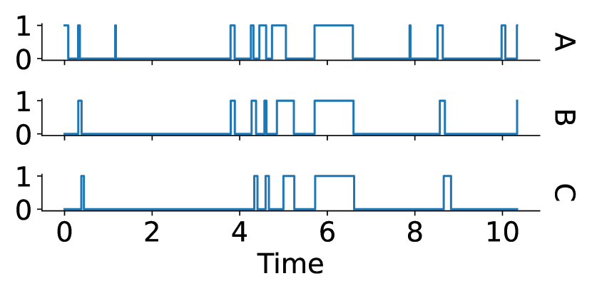
(b)

Figure 4: (a) depicts the graph $\mathcal{G}$ of a CTBN. Its CIMs are in Table A1 in the appendix. Slow processes are represented by solid line nodes, while fast processes are represented by dashed line nodes. Colors describe the most likely sentry state, $s=(s_{1},s_{2},s_{3})$, in this system: If a node is green, the corresponding alarm is 1 (on) in $s$. If a node is red, the corresponding alarm is 0 (off) in $s$. (b) shows an example trajectory from the CTBN represented in Figure 4(a). Each function in the plot represents the evolution of one of the three binary processes, $A$, $B$, and $C$.

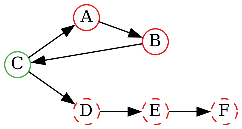
(a)

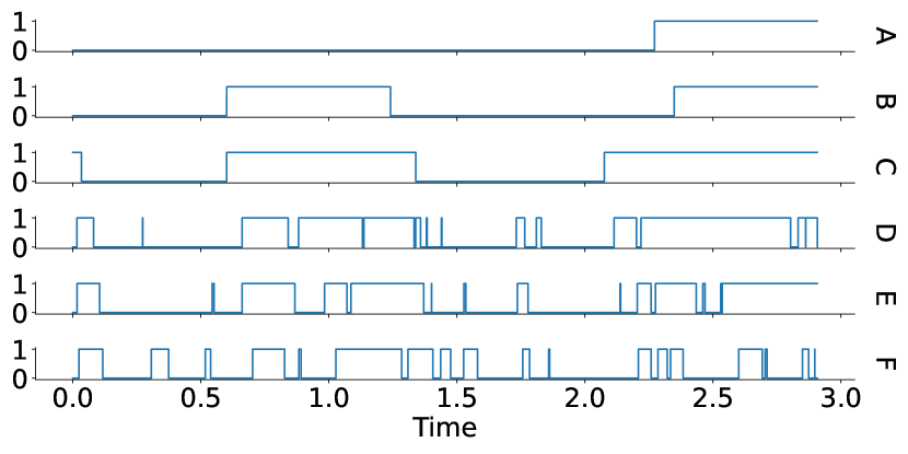
(b)

Figure 5: (a) Graph $\mathcal{G}$ of a CTBN model consisting of six processes. The graph $G$ contains the cycle ($A$, $B$, $C$) as well as the chain ($D$, $E$, $F$). See the caption of Figure 4 for an explanation of the node colors.

Experiment 2

The second synthetic experiment is based on the CTBN shown in Figure 5(a) which consists of a slow cycle ($A$, $B$, $C$) and a fast chain ($D$, $E$, $F$). In this CTBN, the sentry state is expected to be $\{A=0,B=0,C=1,D=0,E=0,F=0\}$. Figure 5(b) shows that this state triggers a fast sequence of alarms in the chain ($D$, $E$, $F$) and a slow sequence of alarms in the cycle ($A$, $B$, $C$). Estimates of the REDNT quantity are shown in Table A3 and they confirm that $\{A=0,B=0,C=1,D=0,E=0,F=0\}$ is a sentry state.

Comparison

We compare the REDNT method to the naive approach proposed in Appendix B. In synthetic data it is easier to identify the two parameters of the naive approach. Each synthetic experiment has only two transition rates and we can let the parameter $\lambda_{ft}$ be the median elapsed time between two consecutive events when combining events of all types. The parameter $\lambda_{mcl}$ can be determined based on the structure of the network. For instance, in the example in Figure 4(a) we expect a cascade to have at least two transitions,

$$\{A=1,B=0,C=0\}\rightarrow\{A=1,B=1,C=0\}\rightarrow\{A=1,B=1,C=1\}.$$

To identify sentry states using the naive approach we should simply identify the cascades of events and compute the fraction of times that observing a specific state coincides with the start of a cascade. As already mentioned in Section 5, we are interested in sentry states with a low number of active alarms. For this reason, we consider only states such that the number of active alarms is less than or equal to the size of the largest parent set in the true graph. The naive approach and the REDNT both produce a list where states are ordered from the most likely sentry state to the least likely. We compare the two approaches with the Jaccard similarity [27] using the $K$ most likely sentry states. We tested our approach on 6 different structures with different numbers of nodes. Results are reported in Figure 6. In every experiment, the two methods share at least one state in their top-two lists. It is important to emphasize that the parameters of the naive method have been set knowing the length of cascades. Conversely, the REDNT method does not require this knowledge in order to identify sentry states.

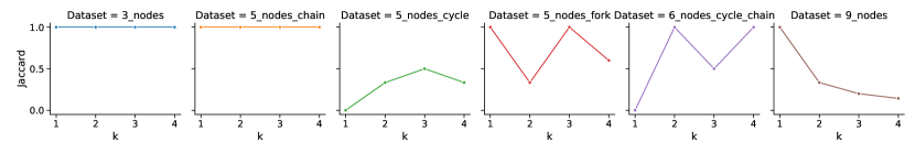
Figure 6: This figure reports the Jaccard similarity@k between the REDNT and the naive approach. The x-axis represents the number of states taken into account from the ordered lists generated by the two methods. The structures of the networks used for the experiments are depicted in Figures 4(a), A1, A2, A3, 5(a), and A4.

ESS Data Set

The last experiment is performed on a real data set provided by the European Spallation Source ERIC (ESS) as described in Section 2. The data set consists of observations of 138 alarm processes from January 2020 to March 2023. No structure was provided, thus we use the score-based structure learning algorithm presented in [32]. We chose not to use the constraint-based algorithm [10] because, in the case of binary variables, it has been shown to be outperformed by the score-based algorithm. The score-based algorithm penalizes the size of the parent sets, leading to sparsity in the graphical structure. For this data, the learned graph is composed of disconnected components. We only present the results of applying the REDNT method for one of them. The most likely sentry state has the alarm SpeedHighFault set to on and everything else set to off (see Figure 7). We observe that the connected component which contains SpeedHighFault is a rooted directed tree, and that SpeedHighFault is the root. This means that an alarm in SpeedHighFault propagates along the directed paths in the tree. A CTBN assumes that at most one event occurs at any point in time. This is reasonable in this application because of the high sampling rate.

The four PressureRatioHighFault alarms in Figure 7 could be verified as consequences of the root cause SpeedHighFault, both from documentation and by an experienced operator. On the other hand, the alarms StateIntervened, CabinetFault, and StateFault were not evident from the documentation and were not expected to be related to the root alarm SpeedHighFault. If these connections are real, this information is relevant to operators as they may look for reasons for this connection and enhance their process understanding. Moreover, the identified root alarm SpeedHighFault can be given a high priority to ensure that the operators will be made aware of a potential cascade starting from this alarm.

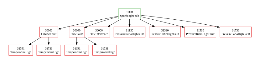
Figure 7: Graph $\mathcal{G}$ of the CTBN learned from the ESS data set. Figure 4 explains the node colors.

The CTBN was learned with no structural input, but using a prior distribution one can provide engineering knowledge to a Bayesian learning method. We believe that the graphical output can easily be shown to and interpreted by engineers; however, user studies are needed to validate this. Results like Propositions 1 and 2 allow a formal interpretation and help us find those components of the system that function independently when accounting for other parts of the machine. Moreover, the sentry states that are identified can be presented to the operators. In the example shown in figure 7 the sentry state is covered by an already existing alarm, but if a more complex sentry state would have been identified then an additional alarm would be needed. Using domain expertise, one can assign appropriate instructions to sentry states and these can be presented to operators when the machine reaches a fault state. When we have learned a CTBN from data, we may also compute the risk of reaching each of the sentry states from the current state. This can be provided to operators in real time to facilitate early mitigation. This should be studied in detail in future work.

Example 5 (Simplified ESS alarm network).

We now return to our running example. This is an example system and it does not correspond to the learned network. Imagine that we start from the state with all alarms off. Assume we have learned from data, using the CTBN framework, that the P1 alarm is very likely to go on if both S4 and T1 alarms are on. Furthermore, assume that P2 is very likely to go on when P1 is on and that P3 is very likely to go on when P2 is on. In this case, the state such that $\text{S4}=1$, $\text{T1}=1$, and such that every other node is zero is likely to be a sentry state. This knowledge can be useful in two ways. First, this can be presented to experts so that they can map common cascades, and their sentry state starting points, to underlying causes using domain knowledge. Second, during operation a warning can be issued when reaching a sentry state, along with the recommended course of action. It is also possible to compute, given the current state, the risk of reaching each of the sentry states within some time interval to facilitate an earlier warning if the expected time from reaching the sentry state to the actual cascade does not suffice for mitigation.

8 Discussion

In this paper we defined the concept of sentry states in CTBNs and we presented a naive approach and a heuristic (REDNT) for identifying such sentry states. The synthetic experiments showed that REDNT can identify the configuration of the network from which a fast sequence of events starts. A key limitation is the fact that the REDNT heuristic is computed for each state and the number of states is exponential in the number of nodes. However, the simplicity of its implementation and the effectiveness showed in the synthetic experiments make the REDNT heuristic attractive. Moreover, only states with few active alarms may be of interest and this reduces the computational cost. The proposed heuristic assigns a score to each state in the state space of a CTBN; a possible extension of this work is the identification of the contribution of each process to the REDNT.

This paper laid the theoretical groundwork for the implementation of online early warning systems based on the identification of sentry states. In practical implementations, a list of sentry states can be provided to domain experts for them to formulate appropriate actions in order to mitigate alarm cascades. This is left for future work. Moreover, the graph representing a learned CTBN indicates how the behavior of each alarm process depends on the states of the other alarm processes. As illustrated in this paper, this graph also represents conditional independences in the system. In future work, we hope to demonstrate that the intended end users, engineers and system operators, also find this graphical tool useful.

8.1 Acknowledgments

The authors would like to thank Per Nilsson for sharing his knowledge about the cryogenics plant and for providing valuable feedback on the work presented in this paper.

Appendix A Graphical information

The following proposition follows from Proposition 4 in [14] and Theorem 2 in [40].

Proposition 3.

If $A$ is ancestral, then the subprocess $\mathbf{X}_{A}=(\mathbf{X}_{i})_{i\in A}$ is a CTBN with transition matrices $Q_{\mathbf{X}_{i}|\text{Pa}(\mathbf{X}_{i})}$ and graph $\mathcal{G}_{A}$.

Proof of Proposition 2.

Note that $A$, $B$, and $C$ must be disjoint. We consider a connecting path between $A$ and $B$ in $(\mathcal{G}_{\text{An}(A\cup B\cup C)})^{m}$ which does not intersect $C$,

$$\mathbf{X}_{i_{0}}-\mathbf{X}_{i_{1}}-\ldots-\mathbf{X}_{i_{m}}.$$

Let $f:\mathbf{X}\rightarrow D$ be the unique map such that if $f(\mathbf{X}_{i})=D_{l}$, then $\mathbf{X}_{i}\in D_{l}$. We consider the walk

$$f(\mathbf{X}_{i_{0}})-f(\mathbf{X}_{i_{1}})-\ldots-f(\mathbf{X}_{i_{m}}).$$

and argue that this walk, or a subwalk, is present in $(\mathcal{D}_{\text{An}(\underline{A}\cup\underline{B}\cup\underline{C})})^{m}$ and is not intersected by $\underline{C}$. Every node on the original walk is in $\text{An}(A\cup B\cup C)$ in $\mathcal{G}$, so every node on the above walk is in $\text{An}(\underline{A}\cup\underline{B}\cup\underline{C})$ in $\mathcal{D}$. We remove nodes such that no adjacent nodes are equal (note that the result is a nontrivial walk). If an edge on the original walk corresponds to a directed edge in $\mathcal{G}$, then it is also in $\mathcal{D}$. Assume it does not correspond to a directed edge on the original walk. It then corresponds to a ‘moral’ edge, $\mathbf{X}_{i_{j}}\rightarrow\mathbf{X}_{k}\leftarrow\mathbf{X}_{i_{j+1}}$ in $\mathcal{G}$, and these must be in different $D_{i}$. In this case, $\mathbf{X}_{i_{j}}-\mathbf{X}_{i_{j+1}}$ is also in $(\mathcal{D}_{\text{An}(\underline{A}\cup\underline{B}\cup\underline{C})})^{m}$. No node can be in $\underline{C}$ on this walk. We can reduce this to a path such that no node is repeated. Note that the end nodes are in $\underline{A}$ and $\underline{B}$, respectively. ∎

Proposition 4.

Let ${D}_{1},\ldots,{D}_{m}$ be the strongly connect components of $\mathcal{G}$. If there are no edges between ${D}_{i}$ and ${D}_{j}$, $i\neq j$, in $\mathcal{G}$, then $\overline{\mathbf{X}}(t)_{D_{i}}\perp\!\!\!\perp\overline{\mathbf{X}}(t)_{D_{j}}\mid\overline{\mathbf{X}}(t)_{p_{i}}$ or $\overline{\mathbf{X}}(t)_{D_{i}}\perp\!\!\!\perp\overline{\mathbf{X}}(t)_{D_{j}}\mid\overline{\mathbf{X}}(t)_{p_{j}}$ where $p_{i}=\bigcup_{D_{k}\in\text{Pa}(D_{i})}D_{k}$ and $p_{j}=\bigcup_{D_{k}\in\text{Pa}(D_{j})}D_{k}$.

Proof.

If there are no edges between any node in ${D}_{i}$ and any node in ${D}_{j}$, then ${D}_{i}$ and ${D}_{j}$ are not adjacent in the condensation of $\mathcal{G}$. The condensation is acyclic, so we can without loss of generality assume that ${D}_{i}$ is not a descendant of ${D}_{j}$. There are no descendants of ${D}_{j}$ in $\text{An}(\{{D}_{i},{D}_{j}\}\cup\text{Pa}({D}_{j}))$ and this means that ${D}_{i}$ and ${D}_{j}$ are separated by $\text{Pa}({D}_{j})$ in $(\mathcal{D}_{\text{An}(\{{D}_{i},{D}_{j}\}\cup\text{Pa}({D}_{j}))})^{m}$ where $\mathcal{D}$ is the condensation of $\mathcal{G}$. The result follows from Propositions 2 and 1. ∎

Appendix B Cascade Identification

Informally, a cascade of events is a fast sequence of transitions; where fast is relative to the rest of the transitions that are observable during the evolution of the process. Starting from this informal definition, we can develop a naive approach to identifying such cascades in a trajectory. First of all we need to identify two quantities: - $\lambda_{ft}$: the fast threshold determines when two consecutive transitions are considered to occur fast. - $\lambda_{mcl}$: the minimum cascade length determines the minimum number of fast consecutive events to be considered a cascade.

Given the two parameters the identification procedure consists of iterating over the entire trajectory and identifying subsets of consecutive transitions with length at least $\lambda_{mcl}$ and with a transition time between each pair of consecutive events of less than $\lambda_{ft}$. This approach can also be used to identify a sentry state. Indeed, once a cascade of events has been identified, the sentry state is the state from which the cascade begins.

The main limitation of this approach is the difficulty of identifying the correct parameters as it requires knowing in advance common durations and sizes of event cascades.

In addition, we define two simple quantities: Naive Count - the number of times a state starts a cascade, and Naive Score - the fraction of times that observing a specific state coincides with the start of a cascade.

Appendix C Synthetic Experiments

A	0	1		A	B	0	1		B	C	0	1
0	-1.0	1.0		0	0	-0.1	0.1		0	0	-0.1	0.1
1	5.0	-5.0			1	15.0	-15.0			1	15.0	-15.0
				1	0	15.0	-15.0		1	0	-15.0	15.0
					1	0.1	-0.1			1	0.1	-0.1

Table A1: Conditional Intensity Matrices used for the example in Figure 4(a). Process A has no parents and therefore its transition rate only depends on its own state: If A is in state 0 (off), then its transition rate (to state 1 (on)) is $1.0$. Process B has a single parent, process A. The states of processes A and B determine the transition rate of process B. If A is in state 0 (off) and B is in state 0 (off), then B transitions to state 1 (on) with rate $0.1$. A CTBN is defined from its CIMs and its initial distribution. Its graph illustrates the dependence structure in the CIMs.

A	B	C	EDNT	REDNT	Naive Score	Naive Count
1	0	0	6.316	1.589	0.35	304
1	0	1	6.444	1.359	0.21	13
0	1	0	5.394	1.357	0.16	41
0	0	1	4.740	1.192	0.03	26
0	1	1	5.511	1.163	0.22	153
1	1	0	6.173	1.145	0.08	57
1	1	1	5.455	1.0	0.03	19
0	0	0	3.976	1.0	0.02	24

Table A2: Values of EDNT, REDNT, Naive Score, and Naive Count for the CTBN depicted in Figure 4(a). Higher values of REDNT indicate CTBN states that are more likely to be sentry states. One should note that high-scoring states with few alarms (bold rows) are more interesting in our application as they correspond to states that occur before strong cascading behavior.

A	B	C	D	E	F	EDNT	REDNT	Naive Score	Naive Count
0	0	1	0	0	0	12.98	1.46	0.24	2172
0	0	0	1	0	0	11.33	1.28	0.25	2156
0	1	0	0	0	0	10.76	1.21	0.04	848
0	0	0	0	1	0	10.75	1.21	0.14	1533
1	0	0	0	0	0	10.24	1.15	0.02	341
0	0	0	0	0	1	9.90	1.12	0.03	651
0	0	0	0	0	0	8.87	1.0	0.01	426

Table A3: Values of EDNT, REDNT, Naive Score, and Naive Count of the states with at most one active alarm for the CTBN depicted in Figure 5(a).

Figure A1: Graph $\mathcal{G}$ of a CTBN model consisting of a chain of five processes.

Figure A2: Graph $G$ of a CTBN model consisting of five processes, including a cycle.

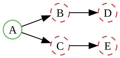
Figure A3: Graph $\mathcal{G}$ of a CTBN model consisting of five processes. The graph $\mathcal{G}$ contains a bifurcation after the root node $A$.

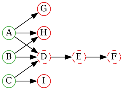
Figure A4: Graph $\mathcal{G}$ of a CTBN model consisting of nine processes and with a more complex structure. The sentry state has three active alarms.

References

- [1] E. Acerbi, E. Viganò, M. Poidinger, A. Mortellaro, T. Zelante, and F. Stella. Continuous Time Bayesian Networks Identify Prdm1 as a Negative Regulator of TH17 Cell Differentiation in Humans. Scientific Reports, 6:23128, 2016.
- [2] Haniyeh Seyed Alinezhad, Mohammad Hossein Roohi, and Tongwen Chen. A review of alarm root cause analysis in process industries: Common methods, recent research status and challenges. Chemical Engineering Research and Design, 2022.
- [3] Samaneh Aminikhanghahi and Diane J Cook. A survey of methods for time series change point detection. Knowledge and information systems, 51(2):339–367, 2017.
- [4] David F Anderson and Thomas G Kurtz. Continuous time markov chain models for chemical reaction networks. In Design and analysis of biomolecular circuits: engineering approaches to systems and synthetic biology, pages 3–42. Springer, 2011.
- [5] Rajeevan Arunthavanathan, Faisal Khan, Salim Ahmed, and Syed Imtiaz. Autonomous fault diagnosis and root cause analysis for the processing system using one-class svm and nn permutation algorithm. Industrial & Engineering Chemistry Research, 61(3):1408–1422, 2022.
- [6] F Ball, RK Milne, and GF Yeo. Multivariate semi-markov analysis of burst properties of multiconductance single ion channels. Journal of Applied Probability, 39(1):179–196, 2002.
- [7] Juraj Bergman, Dominik Schrempf, Carolin Kosiol, and Claus Vogl. Inference in population genetics using forward and backward, discrete and continuous time processes. Journal of Theoretical Biology, 439:166–180, 2018.
- [8] Martin Bicher, Matthias Wastian, Dominik Brunmeir, and Niki Popper. Review on monte carlo simulation stopping rules: How many samples are really enough? Simul. Notes Eur., 32(1):1–8, 2022.
- [9] Jerome V Braun and Hans-Georg Muller. Statistical methods for DNA sequence segmentation. Statistical Science, pages 142–162, 1998.
- [10] Alessandro Bregoli, Marco Scutari, and Fabio Stella. A constraint-based algorithm for the structural learning of continuous-time bayesian networks. International Journal of Approximate Reasoning, 138:105–122, 2021. URL: https://www.sciencedirect.com/science/article/pii/S0888613X21001304, doi:10.1016/j.ijar.2021.08.005.
- [11] Giulia Cencetti, Federico Battiston, Bruno Lepri, and Márton Karsai. Temporal properties of higher-order interactions in social networks. Scientific reports, 11(1):7028, 2021.
- [12] Deepayan Chakrabarti, Yang Wang, Chenxi Wang, Jurij Leskovec, and Christos Faloutsos. Epidemic thresholds in real networks. ACM Transactions on Information and System Security (TISSEC), 10(4):1–26, 2008.
- [13] Daryl J Daley, David Vere-Jones, et al. An introduction to the theory of point processes: volume I: elementary theory and methods. Springer, 2003.
- [14] Vanessa Didelez. Graphical models for composable finite markov processes. Scandinavian Journal of Statistics, 34(1):169–185, 2007.
- [15] EPICS. The experimental physics and industrial control system. Last accessed 2023-04-25. URL: https://epics-controls.org/about-epics/.
- [16] ESS. European spallation source. Last accessed 2023-04-25. URL: https://europeanspallationsource.se/about.
- [17] Xianping Guo and Onésimo Hernández-Lerma. Continuous-time markov decision processes. In Continuous-Time Markov Decision Processes, pages 9–18. Springer, 2009.
- [18] B.R. Hollifield and E. Habibi. Alarm Management: A Comprehensive Guide : Practical and Proven Methods to Optimize the Performance of Alarm Management Systems. International Society of Automation, 2011. URL: https://books.google.se/books?id=UuSMswEACAAJ.
- [19] Jinqiu Hu, Laibin Zhang, Zhansheng Cai, Yu Wang, and Anqi Wang. Fault propagation behavior study and root cause reasoning with dynamic Bayesian network based framework. Process Safety and Environmental Protection, 97:25–36, 2015.
- [20] Srinivasan M Iyer, Marvin K Nakayama, and Alexandros V Gerbessiotis. A markovian dependability model with cascading failures. IEEE Transactions on Computers, 58(9):1238–1249, 2009.
- [21] David Kempe, Jon Kleinberg, and Éva Tardos. Maximizing the spread of influence through a social network. In Proceedings of the ninth ACM SIGKDD international conference on Knowledge discovery and data mining, pages 137–146, 2003.
- [22] Theodoros Lappas, Evimaria Terzi, Dimitrios Gunopulos, and Heikki Mannila. Finding effectors in social networks. In Proceedings of the 16th ACM SIGKDD international conference on Knowledge discovery and data mining, pages 1059–1068, 2010.
- [23] Hyunju Lee and Ji Hwan Cha. Point process approach to modeling and analysis of general cascading failure models. Journal of Applied Probability, 53(1):174–186, 2016.
- [24] Morten Lind. An overview of multilevel flow modeling. International Electronic Journal of Nuclear Safety and Simulation, 4, 2013.
- [25] Manxia Liu, Fabio Stella, Arjen Hommersom, Peter J. F. Lucas, Lonneke Boer, and Erik Bischoff. A comparison between discrete and continuous time bayesian networks in learning from clinical time series data with irregularity. Artif. Intell. Medicine, 95:104–117, 2019. doi:10.1016/j.artmed.2018.10.002.
- [26] Jyotiprasad Medhi. Stochastic models in queueing theory. Elsevier, 2002.
- [27] Allan H Murphy. The finley affair: A signal event in the history of forecast verification. Weather and forecasting, 11(1):3–20, 1996.
- [28] Upama Nakarmi and Mahshid Rahnamay-Naeini. A markov chain approach for cascade size analysis in power grids based on community structures in interaction graphs. In 2020 International Conference on Probabilistic Methods Applied to Power Systems (PMAPS), pages 1–6. IEEE, 2020.
- [29] Upama Nakarmi, Mahshid Rahnamay Naeini, Md Jakir Hossain, and Md Abul Hasnat. Interaction graphs for cascading failure analysis in power grids: A survey. Energies, 13(9):2219, 2020.
- [30] Praneeth Netrapalli and Sujay Sanghavi. Learning the graph of epidemic cascades. ACM SIGMETRICS Performance Evaluation Review, 40(1):211–222, 2012.
- [31] Uri Nodelman, Christian R Shelton, and Daphne Koller. Continuous time Bayesian networks. In Proceedings of the Eighteenth Conference on Uncertainty in Artificial Intelligence (UAI2002), 2002.
- [32] Uri D Nodelman. Continuous time Bayesian networks. PhD thesis, Stanford University, 2007.
- [33] Judea Pearl. Probabilistic reasoning in intelligent systems: networks of plausible inference. Morgan Kaufmann, 1988.
- [34] Mahshid Rahnamay-Naeini, Zhuoyao Wang, Nasir Ghani, Andrea Mammoli, and Majeed M Hayat. Stochastic analysis of cascading-failure dynamics in power grids. IEEE Transactions on Power Systems, 29(4):1767–1779, 2014.
- [35] Marcello Rambaldi, Vladimir Filimonov, and Fabrizio Lillo. Detection of intensity bursts using hawkes processes: An application to high-frequency financial data. Physical Review E, 97(3):032318, 2018.
- [36] Jaxk Reeves, Jien Chen, Xiaolan L Wang, Robert Lund, and Qi Qi Lu. A review and comparison of changepoint detection techniques for climate data. Journal of applied meteorology and climatology, 46(6):900–915, 2007.
- [37] Yaacov Ritov, A Raz, and H Bergman. Detection of onset of neuronal activity by allowing for heterogeneity in the change points. Journal of neuroscience methods, 122(1):25–42, 2002.
- [38] Vicent Rodrigo, Moncef Chioua, Tore Hagglund, and Martin Hollender. Causal analysis for alarm flood reduction. IFAC-PapersOnLine, 49(7):723–728, 2016.
- [39] David Rybach, Christian Gollan, Ralf Schluter, and Hermann Ney. Audio segmentation for speech recognition using segment features. In 2009 IEEE International Conference on Acoustics, Speech and Signal Processing, pages 4197–4200. IEEE, 2009.
- [40] Tore Schweder. Composable markov processes. Journal of applied probability, 7(2):400–410, 1970.
- [41] Christian R Shelton and Gianfranco Ciardo. Tutorial on structured continuous-time Markov processes. Journal of Artificial Intelligence Research, 51:725–778, 2014.
- [42] Charles Truong, Laurent Oudre, and Nicolas Vayatis. Selective review of offline change point detection methods. Signal Processing, 167:107299, 2020.
- [43] Simone Villa and Fabio Stella. Learning continuous time bayesian networks in non-stationary domains. In Proceedings of the Twenty-Seventh International Joint Conference on Artificial Intelligence, IJCAI-18, pages 5656–5660. International Joint Conferences on Artificial Intelligence Organization, 7 2018. doi:10.24963/ijcai.2018/804.
- [44] Yiming Wan, Fan Yang, Ning Lv, Haipeng Xu, Hao Ye, Weichang Li, Peng Xu, Liming Song, and Adam K Usadi. Statistical root cause analysis of novel faults based on digraph models. Chemical Engineering Research and Design, 91(1):87–99, 2013.
- [45] Haoyun Wang, Liyan Xie, Yao Xie, Alex Cuozzo, and Simon Mak. Sequential change-point detection for mutually exciting point processes. Technometrics, pages 1–13, 2022.
- [46] Jeremy C Weiss and David Page. Forest-based point process for event prediction from electronic health records. In Machine Learning and Knowledge Discovery in Databases: European Conference, ECML PKDD 2013, Prague, Czech Republic, September 23-27, 2013, Proceedings, Part III 13, pages 547–562. Springer, 2013.
- [47] Fan Yang, Sirish L Shah, Deyun Xiao, and Tongwen Chen. Improved correlation analysis and visualization of industrial alarm data. ISA transactions, 51(4):499–506, 2012.