The Multivariate Bernoulli detector:
Change point estimation in discrete survival analysis

Abstract

Time-to-event data are often recorded on a discrete scale with multiple, competing risks as potential causes for the event. In this context, application of continuous survival analysis methods with a single risk suffer from biased estimation. Therefore, we propose the Multivariate Bernoulli detector for competing risks with discrete times involving a multivariate change point model on the cause-specific baseline hazards. Through the prior on the number of change points and their location, we impose dependence between change points across risks, as well as allowing for data-driven learning of their number. Then, conditionally on these change points, a Multivariate Bernoulli prior is used to infer which risks are involved. Focus of posterior inference is cause-specific hazard rates and dependence across risks. Such dependence is often present due to subject-specific changes across time that affect all risks. Full posterior inference is performed through a tailored local-global Markov chain Monte Carlo (MCMC) algorithm, which exploits a data augmentation trick and MCMC updates from non-conjugate Bayesian nonparametric methods. We illustrate our model in simulations and on prostate cancer data, comparing its performance with existing approaches.

1 Introduction

Time-to-event data are common in many applications such as finance, medicine and engineering with examples including time to payment, and survival and failure times. Most approaches to survival data consider continuous event times. Nevertheless, it is more and more common to record time to event data on a discrete scale (e.g. patient-reported outcomes, or time to pregnancy measured in number of menstrual cycles it takes a couple to conceive). See Schmid and Berger (2020) for further examples. Discrete recording of the timings of events (Allison, 1982) may occur when time is truly discrete, or when continuous time is partitioned into non-overlapping intervals (corresponding, for instance, to days, weeks, or months) and only the interval in which an event occurs is recorded (King and Weiss, 2021). This special case of interval censoring, usually referred to as grouped time, often leads to ties in the observations in nominally continuous survival data. Time to pregnancy is an example of a truly discrete model since the natural time scale is the number of menstrual cycles. On the other hand, we could consider an underlying continuous survival distribution representing time of conception that could, however, give rise to the same discrete survival distribution after grouping of time (Scheike and Jensen, 1997). In this work, we consider discrete survival models that arise as probabilistic grouped versions of continuous time frailty models from survival analysis (see, e.g., Hougaard, 1986, 1995; Andersen et al., 1993, Chapter IX; Hougaard, Myglegaard, and Borch-Johnsen, 1994; Kalbfleisch and Prentice, 2002). Indeed, direct application of continuous time methods to discretely recorded data may result in biased estimation (Lee et al., 2018).

Moreover, our focus is on discrete survival data in the presence of multiple, competing risks that can cause an event. Traditional analyses often consider a single risk with events due to other risks, e.g. other causes of death, treated as censoring. However, this generally violates the common assumption of independent censoring (Schmid and Berger, 2020). Moreover, such analyses can lead to misestimation of hazards and covariate effects (Andersen et al., 2012).

The two main approaches for competing risks with discrete times are cause-specific hazard functions and the subdistribution hazard model (Schmid and Berger, 2020). The latter is more suitable when interest is in one out of many risks. The first approach usually exploits methods from generalised linear models (GLMs), enabling maximum likelihood estimation, variable selection and other methods from GLMs such as in Tutz (1995) and Möst, Pößnecker, and Tutz (2016). Our work places itself within this approach, focussing on scenarios with few risks which are each of interest and thus consider cause-specific hazards, i.e. a hazard function for each risk. We propose a model for discrete time-to-event data under competing risks with flexible yet simple dependence across risks by building on recent advances in multivariate change point analysis.

A characteristic of traditional discrete survival models as compared to GLMs is that they present unconstrained baseline hazards. This leads to a large number of parameters to estimate and, as a consequence, to unstable estimation, especially if for certain time points the number of events is small. To improve stability, regularisations of hazard functions have been proposed, for example, imposing a polynomial form (McCall, 1996) or smoothing splines (Luo, Kong, and Nie, 2016; Heyard et al., 2019) and penalising innovations across time (Möst et al., 2016). Fahrmeir and Wagenpfeil (1996) and King and Weiss (2021) employ random walks to smooth the hazard function. In all these works, cause-specific baseline hazards are treated independently. Vallejos and Steel (2017) focus on risk-specific covariate selection, still assuming independence across risks. On the other hand, dependence across risks is plausible since multiple hazards can be affected by changes to the individual across time, and as such should be incorporated in the model.

The main methodological contribution of this work is modelling explicit and interpretable dependence across risks. To this end, we introduce a multivariate change point model for the baseline hazards. Change point models are attractive for two reasons (Kozumi, 2000). Firstly, they are effective in reducing the number of parameters and consequently favouring parsimony. Secondly, there are typically many observations at the smallest survival times, with potentially widely varying frequencies requiring a flexible structure in the hazard rate, while often simpler hazard functions are more appropriate at larger times where events are more sparse. Change points can accommodate such variation in complexity. We consider a Bayesian model where we assign a prior on the number of overall, i.e. not cause-specific, change points. Conditionally on this number, we specify a prior on the time location of the change points, inducing marginal dependence among them. For each overall change point, we place a Multivariate Bernoulli prior on which risks are involved, i.e. the cause-specific change points. Note that the Multivariate Bernoulli has been used in time series without prior dependence between overall change points (Dobigeon, Tourneret, and Davy, 2007; Harlé et al., 2016). Following Harlé et al. (2016), we refer to our approach as the Multivariate Bernoulli detector.

Change points have been widely studied in continuous survival analysis (e.g. Matthews and Farewell, 1982; Goodman, Li, and Tiwari, 2011) but less so in the discrete case: Kozumi (2000) considers a single risk modelled via a Markov chain with a prespecified number of change points. Instead, we learn the number of change points from the data. Wang and Ghosh (2007) use posterior predictive checks for change point detection with posterior computation enabled by a conjugate Dirichlet prior on the hazards. They do not include covariates in the model as this would lead to loss of conjugacy and increased computational cost.

Further features of our method include the ability of testing for the presence and location of change points using Bayes factors, and cause-specific variable selection, thanks to the modularity of our approach. The modularity is due to a Gaussian augmented likelihood based on data augmentation for logistic regression (Frühwirth-Schnatter and Frühwirth, 2007). Data augmentation is also exploited to devise efficient Markov chain Monte Carlo (MCMC) schemes for posterior inference. Moreover, such schemes rely also on the connections between the change point models and Bayesian nonparametrics (Martínez and Mena, 2014), allowing for more global updates. Combination of these ideas leads to an effective local-global MCMC scheme.

The paper is structured as follows. Section 2 introduces the model. Section 3 investigates its performance in simulations. Section 4 discusses an application to prostate cancer data. Section 5 compares our approach with existing ones. We conclude the paper in Section 6.

2 Model

2.1 Set-up and notation

We follow the notation in Tutz and Schmid (2016). Let $T_{i}$ denote the time to event for individual $i\in\{1,\dots,n\}$ where $n$ is the number of individuals. In the discrete-time setting, $T_{i}\in\{1,\dots,t_{\max}+1\}$ for some maximum time $t_{\max}$. The random variable $T_{i}$ can for instance arise as the discretisation, also known as grouping (Kalbfleisch and Prentice, 2002), of a latent continuous time $T_{i}^{c}$ into $t_{\max}+1$ intervals $[0,a_{1}),\,[a_{1},a_{2}),\,\dots,\,[a_{t_{\max}},\infty)$. In this case there is a one-to-one correspondence between the set of integers $\{1,\dots,t_{\max}+1\}$ and the intervals of the real line where the continuous-time random variables $T^{c}_{i}$ are defined. As such, the interpretation of $T_{i}=t_{\max}+1$ is similar to censoring, in the sense that the event will occur at time $t>t_{\max}$ and $t_{\max}+1$ is simply a “latent time” that groups together individuals for which it is known that the even has not occurred up to time $t_{\max}$. The time-to-event distribution is usually characterised by the overall hazard function $\lambda(t\mid\theta_{i})={P(T_{i}=t\mid T_{i}\geq t,\theta_{i})}={P\{T_{i}^{c}\in[a_{t-1},a_{t})\mid T_{i}^{c}\geq a_{t-1},\theta_{i}\}}$ for some vector of parameters $\theta_{i}$.

Additionally, we assume that observations are subject to censoring. That means that only a portion of the observed times can be considered as exact survival times. Let $C_{i}$ be the censoring time of individual $i$. $C_{i}$ assumes values in $\{1,\dots,t_{\max}\}$, with $T_{i}$ and $C_{i}$ independent (random censoring). Moreover, we assume that the censoring mechanism is non-informative, i.e. it does not depend on any parameters used to model the event times (Schmid and Berger, 2020). Let $\delta_{i}=\mathds{1}[T_{i}\leq C_{i}]$ be a censoring indicator, where $\mathds{1}[\cdot]$ denotes the indicator function, and $t_{i}=\min(T_{i},C_{i})$ the observed time.

We consider competing risks with $m$ different types of events. For instance, the events can correspond to death due to $m$ different causes. Then, $R_{i}\in\{1,\dots,m\}$ denotes the event type experienced by individual $i$ at time $T_{i}$, for which we observe a value $r_{i}$ only in the absence of censoring, i.e. $\delta_{i}=1$. Finally, the cause-specific hazard function is ${\lambda_{r}(t\mid\theta_{i})}={P(T_{i}=t,\,R_{i}=r\mid T_{i}\geq t,\theta_{i})}$ such that $\lambda(t\mid\theta_{i})=\sum_{r=1}^{m}{\lambda_{r}(t\mid\theta_{i})}$.

2.2 Rationale behind modelling strategy

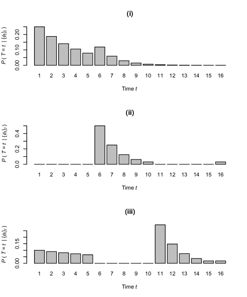
Figure 1: Probability mass function of the Time-Varying Geometric distribution: Visualisations of (1) with $t_{\max}=15$ and success probabilities (i) $\phi_{t}=0.25$ for $t\leq 5$ and $\phi_{t}=0.5$ otherwise; (ii) $\phi_{t}=0$ for $t\leq 5$ or $t\geq 11$, and $\phi_{t}=0.5$ otherwise; (iii) $\phi=0.1$ for $t\leq 5$, $\phi_{t}=0.5$ for $t\geq 11$ and $\phi_{t}=0$ otherwise.

In the uncensored ($\delta=1$) single-risk ($m=1$) case, the distribution of the time to event in the discrete case is a Time-Varying Geometric distribution (Landau and Zachmann, 2019) with time-varying success probability $\phi_{t}=\lambda(t\mid\theta)$, i.e.

$$P(T=t\mid\{\phi_{l}\}_{l})=\begin{cases}\phi_{t}\,\prod_{l=1}^{t-1}(1-\phi_{l}),\quad&t=1,\dots,t_{\max}\\ \prod_{l=1}^{t-1}(1-\phi_{l}),\quad&t=t_{\max}+1\end{cases}$$ (1)

The Time-Varying Geometric is fully flexible in that it can represent any distribution on $\{1,\dots,t_{\max}+1\}$ by appropriately choosing $\phi_{t}$ (Mandelbaum, Hlynka, and Brill, 2007). It is analogous to the piecewise exponential distribution in continuous survival analysis (Gamerman, 1991), if we assume a change point model for the $\phi_{t}$. See Figure 1 for widely varying realisations of the distribution for certain $\{\phi_{t}\}_{t}$. This flexibility should be taken into account when inferring $\phi_{t}$. It relates to the potential lack of stability of unconstrained estimation of baseline hazards mentioned in Section 1. For instance, there is a separate parameter $\phi_{t}$ for each time point, but we might not have observed an event at each time point. To avoid such overpameterisation, some subsequent $\phi_{t}$ can be assumed to be equal to each other, as in Figure 1, resulting in a change point model: a change point is a time $t$ for which $\phi_{t}\neq\phi_{t-1}$. Moreover, given the flexibility of the Time-Varying Geometric, different combinations of $\{\phi_{t}\}$ can lead to a satisfactory fit of a data set, leading to identifiability problems. As such, we impose prior regularisation by a priori shrinking the value of $\phi_{t}$ towards zero. We further motivate our prior choice in the following simulation study.

We simulate $n=500$ times $t_{i}$ from (1) with $t_{\max}=1000$ using two different settings for $\phi_{t}$. We consider a scenario without change points with $\phi_{t}=0.5$, and a scenario with a single change point given by $\phi_{t}=0.5$ for $t\leq 4$ and $\phi_{t}=0.25$ for $t\geq 5$. For this last scenario, we also consider the data after removal of observations with $t_{i}=7$, which we discuss in Section 2.4.1 in relation to the prior constraints on change point location. To understand how the prior on $\phi_{t}$ can affect inference on change points, we compare two priors within a Bayesian change point model defined as follows: we specify a uniform prior over all possible change point configurations among the $\phi_{t}$. Let $\phi_{\ell}^{\star}$ denote the unique value of $\phi_{t}$ over each time interval delimited by the change points. Conditionally on a change point configuration, we choose a prior on $\phi_{\ell}^{\star}$. Then, the likelihood in (1) completes the model. We fit this model with $t_{\max}=\max_{i}t_{i}$, such that $t_{\max}=9$ for the data with no change point and $t_{\max}=14$ for the data with a change point. We compare posterior inference obtained with a uniform prior, $\phi_{\ell}^{\star}\sim\mathcal{U}(0,1)$, and with a prior that shrinks the parameters towards zero, $\phi_{\ell}^{\star}\sim\mathrm{Beta}(0.01,1)$.

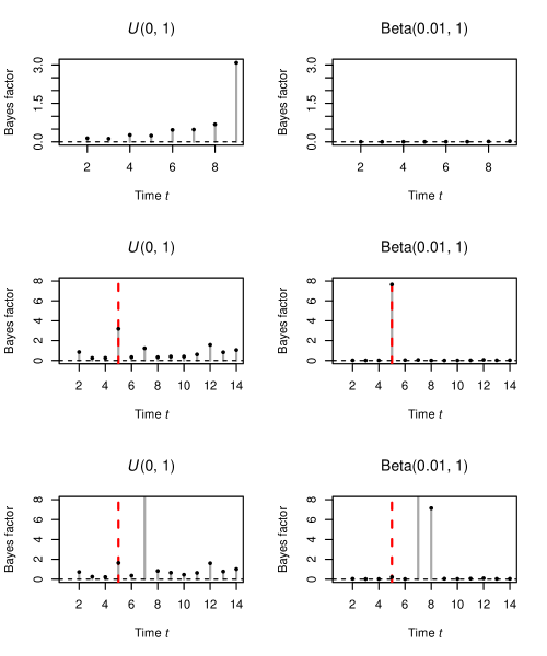
Figure 2: Time-Varying Geometric simulation: Bayes factors for the presence of a change point with a uniform prior (left column, $\phi_{\ell}^{\star}\sim\mathcal{U}(0,1)$) and regularisation towards zero (right column, $\phi_{\ell}^{\star}\sim\mathrm{Beta}(0.01,1)$) when simulating data without (top row) and with (middle and bottom rows) a change point. The bottom row uses the data from the middle row without the observations with $t_{i}=7$. The grey lines with black dots on top indicate the Bayes factors, some of which are outside the plotting range. The dashed lines are drawn in correspondence of the true change point.

Figure 2 shows the inference on change points in terms of the Bayes factors for a change point at each time $t$. The uniform prior (left column) leads to the detection of too many change points, especially at larger $t$. Regularisation towards zero using $\phi_{\ell}^{\star}\sim\mathrm{Beta}(0.01,1)$ (right column) yields more accurate posterior inference without spurious change points (in the case of complete data: we discuss the bottom plots in Section 2.4.1).

2.3 Likelihood

We assume independence across individuals such that the likelihood is a product over individual-specific terms. For ease of explanation, we consider the likelihood contribution of one individual and drop subscripts $i$ in the remainder of this section unless otherwise specified. Under the assumption that $C$ is independent of $T$ and $\theta$, the likelihood for $\theta$ is given by

$$P(T=t,\,R=r\mid\theta)^{\delta}\,P(T>t\mid\theta)^{1-\delta}\\ =\lambda_{r}(t\mid\theta)^{\delta}\,\prod_{l=1}^{t-\delta}\{1-\lambda(l\mid\theta)\}$$ (2)

Here, we specify $\lambda_{r}(t\mid\theta)$ and thus $\lambda(t\mid\theta)$ according to the multinomial logit model which is the most popular for categorical responses (Tutz and Schmid, 2016). Specifically, ${\lambda_{r}(t\mid\theta)}=\exp(\eta_{rt})/\{1+\sum_{\rho=1}^{m}\exp(\eta_{\rho t})\}$ where $\eta_{rt}=\alpha_{rt}+\bm x^{\top}\bm\beta_{r}$ is a cause- and time-specific linear predictor, and $\theta=\{\eta_{rt}\}$. The intercept $\alpha_{rt}$ represents the cause-specific baseline hazard. The $p$-dimensional vector $\bm\beta_{r}$ consists of the cause-specific regression coefficients of the covariates in the $p$-dimensional vector $\bm x$. Note that, when $r=1$ and $\delta=1$, $\lambda_{r}(t\mid\theta)$ corresponds to $\phi_{t}$ defined in Section 2.2 and the considerations on prior specification there discussed will be relevant when building a change point model on $\alpha_{rt}$.

2.4 The Multivariate Bernoulli detector

We propose a model on the baseline hazards that is flexible, yet has interpretable structure. Specifically, the sequence $\alpha_{r1},\ldots,\alpha_{r,t_{\max}}$ is set to follow a step function. We do so through a change point model with dependence across risks $r$. In our set-up, a change point corresponds to a time point where the hazard of at least one risk $r$ changes. We specify a hierarchical prior on the change points which has three main components: (i) a prior on the number of change points; (ii) a prior on the location of change points; (iii) and a prior on which risks (at least one) have a change point at that particular time location, given that a change point at time $t$ occurs.

2.4.1 Prior specification on overall change points

In this section, we describe prior specification on the number and location of change points. Let $\bm\alpha_{t}=(\alpha_{1t},\dots,\alpha_{mt})^{\top}$. Then, $\gamma_{t}=\mathds{1}[\bm\alpha_{t}\neq\bm\alpha_{t-1}]$ indicates whether there is an overall change point at $t\in\{1,\dots,t_{\max}\}$, i.e. if the hazard of at least a risk changes at time $t$. Furthermore, $K=\sum_{t\in\mathcal{T}}\gamma_{t}$ denotes the number of change points. Here $\mathcal{T}$ defines the set of possible change point locations. We specify the prior on $\bm\gamma=(\gamma_{1},\dots,\gamma_{t_{\max}})^{\top}$ hierarchically, by specifying a prior $p(K)$ on the number of change points and then $p(\bm\gamma\mid K)$ as this provides explicit regularisation on $K$: i.i.d. $\gamma_{t}$ would imply a binomial distribution on $K$.

To motivate the next model development, consider the bottom plots in Figure 2 where two observations with $t_{i}=7$ out of 500 are not used when inferring change points. Then, the lack of observations at time $t=7$ results in spurious change points at that time location and the next. We restrict our inference to avoid such sensitivity to a few observations: to aid identifiability, considering the flexibility of the underlying Time-Varying Geometric distribution, we only allow change points for a subset of times $\mathcal{T}\subset\{1,\dots,t_{\max}\}$ such that $\gamma_{t}=0$ if $t\notin\mathcal{T}$. Firstly, as it is typical in change point applications, we do not allow change points at the support boundary, in our case $t=1$ and $t=t_{\max}$. Moreover, we do not allow a change point at time $t$ if both $t$ and $t-1$ have no observed events as the data lack information on which of the two time points would be a change point. Also, we do not allow change points at a time $t$ with no observed events if both neighbouring times $t-1$ and $t+1$ have observed events, because this would lead to spurious change points due to the flexibility of the underlying Time-Varying Geometric, as seen in Figure 2 (bottom row). Indeed, without this constraint the model would in general favour a very low $\phi_{t}$ as no event has been observed at time $t$ and then rescale all the subsequent $\phi_{l}$, $l>t$. On the other hand, we prefer to introduce parsimony in the estimation of change points to improve interpretability.

We assume a Geometric distribution with success probability $\pi_{K}$ truncated to $K\leq|\mathcal{T}|$ as prior on the number of change points. We denote such prior as $\mathrm{Geo}_{|\mathcal{T}|}(\pi_{K})$. For the locations of overall change points given $K$, we use the uniform distribution on possible configurations $p(\bm\gamma\mid K)=1/\binom{|\mathcal{T}|}{K}$. In summary, the joint prior on the number and location of change points has a hierarchical specification:

$$p(K,\bm\gamma)=p(K)\,p(\bm\gamma\mid K)$$

2.4.2 Cause-specific change point configuration

In this section, we discuss the prior on which risks present a jump in the hazard, given the vector $\bm\gamma$. Let $z_{rt}=\mathds{1}[\alpha_{rt}\neq\alpha_{r(t-1)}]$ be an indicator variable denoting if a change point occurs at time $t$ for risk $r$. If there is no change point at $t$ for any $r$, then $\gamma_{t}=0$ and $z_{rt}=0$. If $\gamma_{t}=1$, then $z_{rt}=1$ for at least one $r$.

Let $\bm z_{t}=(z_{1t},\dots,z_{mt})$. Conditionally on $\gamma_{t}=1$, we assume that $\bm z_{t}$ follows a Multivariate Bernoulli distribution (e.g. Teugels, 1990). An $m$-dimensional binary vector $\bm z_{t}$ can assume $2^{m}$ possible values corresponding to a combination of $z_{rt}\in\{0,1\}$. The Multivariate Bernoulli distribution is then parameterised by a $2^{m}$-dimensional vector, whose elements correspond to the probability of each particular outcome (i.e. configuration). In our case, when modelling $\bm z_{t}$ given $\gamma_{t}=1$, we exclude the configuration of all zeros, i.e. $z_{rt}=0$ for every $r$. Thus, $\bm z_{t}$ can assume only $2^{m}-1$ possible values. We denote such distribution as $\mathrm{Ber}_{0}(\bm\psi)$, where $\bm\psi$ denotes the $(2^{m}-1)$- dimensional vector of configuration probabilities. In summary, the prior specification for $\bm z_{t}$ is

$$\bm z_{t}\mid\gamma_{t}\sim\left\{\begin{array}[]{lcl}\mathrm{Ber}_{0}(\bm\psi)&&\mbox{if }\gamma_{t}=1\\ \delta_{\bm 0}&&\mbox{if }\gamma_{t}=0\end{array}\right.$$

where $\delta_{\bm 0}$ is a point mass at the zero vector. We refer to the joint prior on $(K,\bm\gamma,\bm z)$ as Multivariate Bernoulli detector, where $\bm z=\{\bm z_{t}\}_{t=1}^{t_{\max}}$.

2.5 Further prior specification

Model specification is completed by specifying independent prior distributions on $\alpha_{rt}$ and $\bm\beta_{r}$. We specify a prior on $\alpha_{rt}$ conditionally on the number and location of change points. Since $\bm\alpha_{r}=(\alpha_{r1},\ldots,\alpha_{rt_{\max}})^{\top}$ is a a step function for each risk $r$, assuming constant values between change points, let $\alpha_{r\ell}^{\star}$ denote the unique value of $\alpha_{rt}$ over each time interval for risk $r$. Note that for each risk a change point can be activated or not, with the only constraint that a change point needs to be activated for at least one risk. We assume $\alpha_{r\ell}^{\star}\sim\mathcal{N}(\mu_{\alpha},\sigma^{2}_{\alpha})$ independently across $\ell$ and $r$.

Furthermore, to identify important effects, we assume a variable selection prior for the regression coefficients, $\bm\beta_{r}=(\beta_{r1},\dots,\beta_{rp})^{\top}$, which allows for risk-specific variable selection. Here, we consider a spike-and-slab prior (Mitchell and Beauchamp, 1988): $\beta_{rj}\sim\pi_{\beta}\,\mathcal{N}(0,\sigma^{2}_{\beta})+(1-\pi_{\beta})\,\delta_{0}$ where $\pi_{\beta}$ is the prior inclusion probability. We use the hyperprior $\pi_{\beta}\sim\mathcal{U}(0,1)$. We note that other possible prior choices are available in the literature to perform variable selection, such as shrinkage priors (Bhadra et al., 2019), which offer computational advantages, at the cost of depending on arbitrary thresholds to identify relevant effects.

In the simulation study and the application on prostate cancer data, we set the hyperparameter as follows: $\sigma^{2}_{\beta}=1$, $\pi_{K}=0.5$, all elements of $\bm\psi$ equal to $1/(2^{m}-1)$, $\mu_{\alpha}=-9$ and $\sigma^{2}_{\alpha}=3$. The particular prior choice for $\alpha_{r\ell}^{\star}$ derives from the interpretation of the model in terms of the Time-Varying Geometric. In Section 2.2, we highlighted the importance of shrinking the probabilities $\phi_{t}$ towards zero. This is equivalent, in absence of covariates, to shrinking $\exp(\alpha^{\star}_{r\ell})/\{1+\exp(\alpha^{\star}_{r\ell})\}$ towards zero and, consequently, $\alpha^{\star}_{r\ell}$ towards $-9$. Roughly speaking, a $\mathcal{N}(-9,3)$ on $\alpha^{\star}_{r\ell}$ is equivalent to a $\mathrm{Beta}(0.01,1)$ prior on $\phi_{t}$, which is shown to have a good performance in Section 2.2.

2.6 Posterior computation using local-global MCMC

To devise an MCMC scheme to perform posterior inference, we exploit the representation of the likelihood in (2) as a multinomial logistic regression (Tutz and Schmid, 2016), using a data augmentation trick. This results in the availability of conjugate updates, leading to more efficient mixing and preventing, at the same time, large changes in the configuration of change points, resulting in more effective local moves. The latent variables associated with the data augmentation are highly correlated with the change points, and, as such, it is difficult to explore the change points space conditionally on the latent variables. To counterbalance this drawback, we also devise global moves of change points conditionally on the observed data. Such moves are based on ideas from the Bayesian nonparametric literature (Dahl, 2005; Martínez and Mena, 2014; Creswell et al., 2020).

We refer to the resulting hybrid algorithm as “local-global MCMC” borrowing the terminology from Samsonov et al. (2022). Here, we provide a brief explanation of our MCMC strategy in relation to previous work. Web Appendix LABEL:ap:mcmc details the algorithm.

2.6.1 Local MCMC with data augmentation

We exploit the data augmentation representation of a multinomial logistic regression in terms of Gumbel latent variables by McFadden (1974) and Frühwirth-Schnatter and Frühwirth (2007). Then, the augmented likelihood is Gaussian which enables convenient MCMC updates. Importantly, conditionally on the $z_{rt}$, the $\alpha_{r\ell}^{\star}$ have a Gaussian prior such that they can be integrated out from the augmented posterior, enabling efficient updates of $z_{rt}$ and $\gamma_{t}$ without having to specify Metropolis-Hastings proposals for $\alpha_{r\ell}^{\star}$.

More recently, other augmentations have been proposed in the literature (see, for instance, Held and Holmes, 2006; Frühwirth-Schnatter and Frühwirth, 2010; Polson, Scott, and Windle, 2013; Linderman, Johnson, and Adams, 2015). We do not opt for them because they do not provide a convenient augmented likelihood in the presence of multiple risks.

2.6.2 Global MCMC

We also consider MCMC moves without data augmentation. The augmented data can strongly reflect the change points of the current state of the MCMC chain, resulting in local MCMC updates to the change point parameters $z_{rt}$ and $\gamma_{t}$. Therefore, we alternate between data augmentation and MCMC without augmentation to enable more global change point updates. Specifically, we exploit the fact that change points induce a partition of time into intervals. For this type partition, MCMC schemes are available when the prior on $\alpha_{r\ell}^{\star}$ is conjugate (Martínez and Mena, 2014), which is not the case without augmentation. We thus apply ideas from Bayesian nonparametrics (Dahl, 2005; Creswell et al., 2020) to extend such MCMC to non-conjugate priors. This allows for more global moves at the cost of having to specify Metropolis-Hastings proposals for $\alpha_{r\ell}^{\star}$. Alternating between local and global MCMC steps allows for better mixing and convergence of the algorithm.

2.7 Bayes factor for change points

We now describe a strategy to test for the presence of change points. In particular, we provide a strategy to compute the Bayes factor $B$ for $K=0$ (model $\mathcal{M}^{\star}$, denoting no change points) versus a model with $K\sim p(K)$ (model $\mathcal{M}$) (see Legramanti, Rigon, and Durante, 2022, for a similar example of such model comparison). $B$ is readily computed from MCMC output. Let $\bm y$ denote all the observed data. Then

$$B=\frac{p(\bm y\mid\mathcal{M}^{\star})}{p(\bm y\mid\mathcal{M})}=\frac{p(\bm y\mid K=0)}{p(\bm y)}=\frac{p(\bm y,K=0)}{p(\bm y)\,p(K=0)}=\frac{p(K=0\mid\bm y)}{p(K=0)}$$

where the last ratio is the Savage-Dickey ratio (Dickey, 1971). Here, ${p(K=0\mid\bm y)}$ is readily estimated by the MCMC sample frequency of $K=0$ while $p(K=0)$ is available from the prior.

This scheme can be employed as long as $p(K=0)$ is not too small as it would lead to unstable estimation of $B$ when also $p(K=0\mid\bm y)$ is small (i.e. the MCMC chain visits $K=0$ only rarely). This is not the case in our scenario as $K\sim\mathrm{Geo}_{|\mathcal{T}|}(\pi_{K})$ such that $p(K=0)>\pi_{K}=0.5$.

3 Simulation study

We demonstrate the performance of our approach in simulation studies. We show good performance of our model in the absence of change points in Web Appendix LABEL:ap:null_simulation. Here, focus is on inference in the presence of change points. We simulate $n=300$ observations from the model in Section 2 with $t_{\max}=20$, $m=3$ risks, no covariates ($p=0$) and baseline hazard with two change points: one at $t=6$ involving all three risks and another at $t=13$ affecting only risks 1 and 2. Specifically, $\bm\alpha_{t}=(-9,-9,-9)^{\top}$ before the first change point ($t=1,\dots,5$), $\bm\alpha_{t}=(-4,-3,-3)^{\top}$ between the two change points ($t=6,\dots,12$) and $\bm\alpha_{t}=(-2,-2,-3)^{\top}$ after the second change point ($t=13,\dots$). We consider three scenarios with (i) no censoring beyond those with $T_{i}=t_{\max}+1$, and (ii) 10% and (iii) 50% of the individuals being censored, which are selected at random. For those censored individuals, we sample the censoring time $C_{i}$ uniformly from the set $\{1,\dots,T_{i}-1\}$. We fit our model using 100 000 MCMC iterations, discarding the first 10 000 as burn-in.

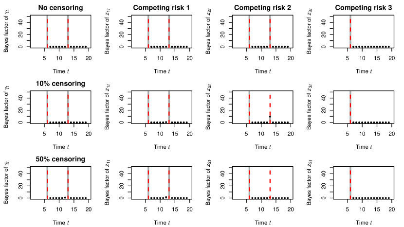
Figure 3: Simulation study: Bayes factors for the presence of a change point for the overall (left column) and cause-specific (other columns) hazard functions. The grey lines with black dots on top indicate the Bayes factors, some of which are outside the plotting range. The dashed lines are drawn in correspondence of the true change points.

We summarise the resulting inference on change points in Figure 3 using the Bayes factor of $\gamma_{t}=1$ over $\gamma_{t}=0$ and $z_{rt}=1$ over $z_{rt}=0$. The Bayes factor is shown only for those times $t\in\mathcal{T}$ at which change points are allowed. Our model recovers both the overall and cause-specific change points with high accuracy in the absence of censoring. With 20% censoring, inference on the relatively minor second change point in the second risk is more uncertain. Finally, this cause-specific change point is missed with 70% censoring. The inference on $\alpha_{rt}$, shown in Web Appendix LABEL:ap:simul_alpha, similarly shows accurate recovery across all risks only for scenarios (i) and (ii) with limited censoring. Web Appendix LABEL:ap:simul_alpha also contains a comparison with the alternative models described in Section 5. The comparison reveals more accurate inference with more certainty for the Multivariate Bernoulli detector with its dependence across risks. Finally, the estimate of the Bayes factor $B$ from Section 2.7 is zero in all three scenarios, which is in line with the presence of change points.

4 Application to prostate cancer data

4.1 Data description and analysis

We apply our model to data on prostate cancer from the Surveillance, Epidemiology, and End Results Program (SEER Program, 2022) with time to death as outcome. Our focus is on prostate cancer patients as they are typically older while prostate cancer has one of the highest survival rates amongst cancers (Siegel et al., 2023). As such, death due to other causes presents a major competing risk for death due to prostate cancer. We therefore consider these $m=2$ competing risks. We include age and ethnicity as covariates.

Here, we consider only subjects diagnosed in the most recent year (2017) to reduce computational cost. Next, we exclude patients with incomplete date information in the database or who have no follow-up, for instance because they were diagnosed upon death. Then only considering those with age and ethnicity recorded in the database, we are left with a data set with $n=49~{}057$ individuals. We consider as $p=2$ covariates (i) age standardised to have zero mean and unit standard deviation, and (ii) an indicator that equals zero for ethnicity “white” and one otherwise.

Time to death $t_{i}$ is discrete in this database as it is recorded in months. Specifically, $t_{i}=1$ corresponds to surviving up to one month and $t_{i}\geq 2$ to surviving between $(t_{i}-1)$ and $t_{i}$ months after diagnosis. Most (45 319 or 92%) survival times are censored, i.e. when an individual is alive at his most recent follow-up visit. Of the observed deaths, 1611 are due to prostate cancer and 2127 due to other causes.

We fit our model with $t_{\max}=\max_{i}t_{i}=36$ months using 100 000 MCMC iterations, discarding the first 10 000 as burn-in.

4.2 Posterior inference on the baseline hazards

We use the MCMC samples for inference on the change point model and its regression coefficients. The estimate of the Bayes factor $B$ from Section 2.7 is zero which suggests the presence of change points. Figure 4 summarises inference on the baseline hazards. The hazard functions decrease rapidly in the first few months after which they stabilise. Then, only the cause-specific hazard function for prostate cancer sees a further decrease after two years. As the time since diagnosis increases, the patient becomes more likely to pass away from other causes.

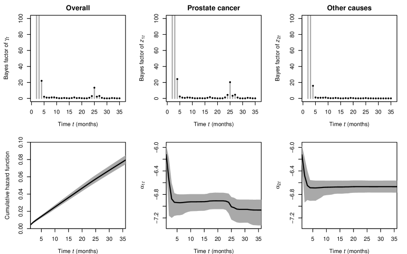
Figure 4: Prostate cancer data: Posterior inference on the overall (left column) and cause-specific (other columns) baseline hazards. The top row visualises the Bayes factors for the presence of a change point. The bottom row shows posterior inference for the cumulative hazard function of a white individual of average age, i.e. $\bm x_{i}=\bm 0$, and the baseline hazard parameter $\alpha_{rt}$. The grey lines with black dots on top indicate the Bayes factors, some of which are outside the plotting range. Black lines represent posterior means and shaded areas demarcate 95% credible intervals.

4.3 Posterior inference on the regression coefficients

The regression coefficients $\beta_{rj}$ capture cause-specific covariate effects on survival time. The spike-and-slab prior provides explicit inference on whether there is a covariate effect through the posterior probability of $\beta_{rj}\neq 0$. These posterior inclusion probabilities equal one in this application. Furthermore, Figure 5 shows that both risks increase with age, with white people surviving longer after diagnosis than other ethnicities.

Figure 5: Prostate cancer data: Posterior means (dot) and 95% credible intervals (lines) of the regression coefficients from our model. Solid lines correspond to prostate cancer risk ($r=1$). Dashed lines correspond to death due to other causes ($r=2$).

5 Comparison with other models

In this section, we compare our results on the cancer data to those obtained from maximum likelihood estimation and a more recent alternative, namely the model by King and Weiss (2021).

5.1 Maximum likelihood estimation

We maximise the likelihood in (2) with respect to $\bm\alpha_{t}$ and $\bm\beta_{r}$ using the R package nnet (Venables and Ripley, 2002) as the likelihood is equivalent to a multinomial logistic regression (Tutz and Schmid, 2016).

The resulting inference is shown in Web Figures LABEL:fig:prostate_nnet_hazard and LABEL:fig:prostate_nnet_regression. The inference for $\bm\alpha_{t}$ is less smooth than from our model, but also shows similarities with a decrease in hazard during the first months and a decrease in the hazard for prostate cancer around two years. The estimates for $\bm\beta_{r}$ are in agreement with our estimates.

5.2 Semi-parametric model by King and Weiss (2021)

We also compare our model with the Bayesian semi-parametric model by King and Weiss (2021), which also involves multiple risk and a flexible model for the hazard function. Similarly, they use a multinomial logit model for discrete survival analysis with competing risks but $\eta_{irt}=\alpha_{rt}+\sum_{\text{quantitative $j$}}f_{\beta rj}(x_{ij})+\sum_{\text{categorical $j$}}\beta_{rjx_{ij}}$ where $\beta_{rjx}$ is a regression coefficient for category $x$ and $\alpha_{tr}=\beta_{0r}+f_{\alpha r}(t)$ for intercepts $\beta_{0r}$, and functions $f_{\alpha r}$ and $f_{\beta rj}$ that are to be inferred. When fitting this model to the prostate cancer data, we set $\eta_{irt}=\alpha_{rt}+f_{\beta r1}(x_{i1})+\beta_{r2x_{i2}}$ where $x_{i1}$ is the individual’s age and $x_{i2}=\mathds{1}[\text{individual's ethnicity is not white}]$. For $\beta_{r2x}$ a priori, $\beta_{r20}=-\beta_{r21}$ with $\beta_{r20}\sim\mathcal{N}(0,1/\nu)$ for some hyperparameter $\nu$. The prior on the intercepts is $p(\beta_{0r})\propto 1$. The functions $f_{\alpha r}$ and $f_{\beta r1}$ are inferred using a Gaussian Markov random field prior. For hyperparameter choice, we follow the recommendations in Appendix C of King and Weiss (2021) for uninformative priors. For instance, we set $\nu=1/16$. We fit the model using the R package brea (King, 2017) using 10 000 burn-in MCMC iterations followed by 100 000 recorded iterations.

The resulting inference is shown in Web Figures LABEL:fig:prostate_brea_hazard and LABEL:fig:prostate_brea_regression. The baseline hazards show a decrease in the first months and, only for prostate cancer, a further decrease around two years, in line with our model. The decrease in the first months is more pronounced in our model, with smaller credible intervals, which might be a result of dependence across risks that King and Weiss (2021) do not consider. The non-linear regression effect of age differs between death due to prostate cancer and due to other causes with a positive effect appearing only at a higher age (above 40) for prostate cancer. Our model also detects a difference in the effect of age between risks. The posterior mean of the difference in risk between white and non-white individuals, i.e. $\beta_{r21}-\beta_{r20}$, is 0.29 (95% credible interval [0.18, 0.40]) for prostate cancer ($r=1$) and 0.16 (95% credible interval [0.06, 0.26]) for death due to other causes ($r=2$), which is similar to the results from our model in Figure 5.

6 Discussion

In this paper, we focus on the estimation of the hazard function of competing risks in the context of discrete survival. We assume a change point model for the hazard function, with cause-specific change points, introducing dependence among change point locations across risks. In our approach, both number and location of change points are random. We refer to our model as Multivariate Bernoulli detector. Dependence across risks provides an attractive way for regularisation of baseline hazards since changes to an individual’s condition across time might affect multiple cause-specific hazards simultaneously. Our approach is widely applicable and interpretable. The data augmentation enables the use of any prior on regression coefficients making the MCMC updates more efficient. The simulation study shows that posterior inference on change points with dependence across risks is effective, with favourable comparisons with a frequentist approach and the Bayesian semi-parametric model by King and Weiss (2021). In the application, such comparisons yield consistent results in terms of both baseline hazards and covariate effects.

Finally, the proposed model can be easily extended to accommodate more complex scenarios, for example, inclusion of recurrent event processes as outcome (see, e.g., King and Weiss, 2021) or of time-varying covariates. In this work, we employ the multinomial logit model which is a popular choice for the analysis of discrete competing risks. It closely relates to multinomial logistic regression and offers computational advantages. Nevertheless, the Multivariate Bernoulli detector can be used with other likelihoods, such as multinomial probit models or multiple time series.

Data availability statement

The data that support the findings of this study are available from the SEER Program. Restrictions apply to the availability of these data, which were used under license for this study. Data are available at www.seer.cancer.gov with the permission of the SEER Program.

Supporting Information

Web Appendices and Figures referenced in Sections 2.6, 3, 4 and 5 are available with this paper’s Supporting Information. The code to implement the model is available at https://github.com/willemvandenboom/mvb-detector.

References

- Allison (1982) Allison, P. D. (1982). Discrete-time methods for the analysis of event histories. Sociological Methodology 13, 61–98.
- Andersen et al. (1993) Andersen, P. K., Borgan, Ø., Gill, R. D., and Keiding, N. (1993). Statistical Models Based on Counting Processes. Springer Series in Statistics. Springer, New York, NY.
- Andersen et al. (2012) Andersen, P. K., Geskus, R. B., de Witte, T., and Putter, H. (2012). Competing risks in epidemiology: Possibilities and pitfalls. International Journal of Epidemiology 41, 861–870.
- Bhadra et al. (2019) Bhadra, A., Datta, J., Polson, N. G., and Willard, B. (2019). Lasso meets horseshoe: A survey. Statistical Science 34, 405–427.
- Creswell et al. (2020) Creswell, R., Lambert, B., Lei, C. L., Robinson, M., and Gavaghan, D. (2020). Using flexible noise models to avoid noise model misspecification in inference of differential equation time series models. arXiv:2011.04854v1.
- Dahl (2005) Dahl, D. B. (2005). Sequentially-allocated merge-split sampler for conjugate and nonconjugate Dirichlet process mixture models. Technical report, Department of Statistics, Texas A&M University.
- Dickey (1971) Dickey, J. M. (1971). The weighted likelihood ratio, linear hypotheses on normal location parameters. The Annals of Mathematical Statistics 42, 204–223.
- Dobigeon et al. (2007) Dobigeon, N., Tourneret, J.-Y., and Davy, M. (2007). Joint segmentation of piecewise constant autoregressive processes by using a hierarchical model and a Bayesian sampling approach. IEEE Transactions on Signal Processing 55, 1251–1263.
- Fahrmeir and Wagenpfeil (1996) Fahrmeir, L. and Wagenpfeil, S. (1996). Smoothing hazard functions and time-varying effects in discrete duration and competing risks models. Journal of the American Statistical Association 91, 1584–1594.
- Frühwirth-Schnatter and Frühwirth (2007) Frühwirth-Schnatter, S. and Frühwirth, R. (2007). Auxiliary mixture sampling with applications to logistic models. Computational Statistics & Data Analysis 51, 3509–3528.
- Frühwirth-Schnatter and Frühwirth (2010) Frühwirth-Schnatter, S. and Frühwirth, R. (2010). Data augmentation and MCMC for binary and multinomial logit models. In Kneib, T. and Tutz, G., editors, Statistical Modelling and Regression Structures, pages 111–132. Springer-Verlag, Berlin, Germany.
- Gamerman (1991) Gamerman, D. (1991). Dynamic Bayesian models for survival data. Journal of the Royal Statistical Society Series C: Applied Statistics 40, 63–79.
- Goodman et al. (2011) Goodman, M. S., Li, Y., and Tiwari, R. C. (2011). Detecting multiple change points in piecewise constant hazard functions. Journal of Applied Statistics 38, 2523–2532.
- Harlé et al. (2016) Harlé, F., Chatelain, F., Gouy-Pailler, C., and Achard, S. (2016). Bayesian model for multiple change-points detection in multivariate time series. IEEE Transactions on Signal Processing 64, 4351–4362.
- Held and Holmes (2006) Held, L. and Holmes, C. C. (2006). Bayesian auxiliary variable models for binary and multinomial regression. Bayesian Analysis 1, 145–168.
- Heyard et al. (2019) Heyard, R., Timsit, J.-F., Essaied, W. I., and Held, L. (2019). Dynamic clinical prediction models for discrete time-to-event data with competing risks—A case study on the OUTCOMEREA database. Biometrical Journal 61, 514–534.
- Hougaard (1986) Hougaard, P. (1986). Survival models for heterogeneous populations derived from stable distributions. Biometrika 73, 387–396.
- Hougaard (1995) Hougaard, P. (1995). Frailty models for survival data. Lifetime Data Analysis 1, 255–273.
- Hougaard et al. (1994) Hougaard, P., Myglegaard, P., and Borch-Johnsen, K. (1994). Heterogeneity models of disease susceptibility, with application to diabetic nephropathy. Biometrics 50, 1178–1188.
- Kalbfleisch and Prentice (2002) Kalbfleisch, J. D. and Prentice, R. L. (2002). The Statistical Analysis of Failure Time Data. John Wiley & Sons, Hoboken, NJ, 2nd edition.
- King (2017) King, A. J. (2017). brea: Bayesian recurrent event analysis. R package version 0.2.0. https://CRAN.R-project.org/package=brea.
- King and Weiss (2021) King, A. J. and Weiss, R. E. (2021). A general semiparametric Bayesian discrete-time recurrent events model. Biostatistics 22, 266–282.
- Kozumi (2000) Kozumi, H. (2000). Bayesian analysis of discrete survival data with a hidden Markov chain. Biometrics 56, 1002–1006.
- Landau and Zachmann (2019) Landau, V. A. and Zachmann, L. J. (2019). tvgeom: an R package for the time-varying geometric distribution. R package version 1.0.1. https://CRAN.R-project.org/package=tvgeom.
- Lee et al. (2018) Lee, M., Feuer, E. J., and Fine, J. P. (2018). On the analysis of discrete time competing risks data. Biometrics 74, 1468–1481.
- Legramanti et al. (2022) Legramanti, S., Rigon, T., and Durante, D. (2022). Bayesian testing for exogenous partition structures in stochastic block models. Sankhya A 84, 108–126.
- Linderman et al. (2015) Linderman, S., Johnson, M. J., and Adams, R. P. (2015). Dependent multinomial models made easy: Stick-breaking with the Pólya-gamma augmentation. In Cortes, C., Lawrence, N., Lee, D., Sugiyama, M., and Garnett, R., editors, Advances in Neural Information Processing Systems, volume 28. Curran Associates, Inc.
- Luo et al. (2016) Luo, S., Kong, X., and Nie, T. (2016). Spline based survival model for credit risk modeling. European Journal of Operational Research 253, 869–879.
- Mandelbaum et al. (2007) Mandelbaum, M., Hlynka, M., and Brill, P. H. (2007). Nonhomogeneous geometric distributions with relations to birth and death processes. TOP 15, 281–296.
- Martínez and Mena (2014) Martínez, A. F. and Mena, R. H. (2014). On a nonparametric change point detection model in Markovian regimes. Bayesian Analysis 9, 823–858.
- Matthews and Farewell (1982) Matthews, D. E. and Farewell, V. T. (1982). On testing for a constant hazard against a change-point alternative. Biometrics 38, 463–468.
- McCall (1996) McCall, B. P. (1996). Unemployment insurance rules, joblessness, and part-time work. Econometrica 64, 647–682.
- McFadden (1974) McFadden, D. (1974). Conditional logit analysis of qualitative choice behavior. In Zarembka, P., editor, Frontiers in Econometrics, Economic Theory and Mathematical Economics, pages 105–142. Academic Press, New York, NY.
- Mitchell and Beauchamp (1988) Mitchell, T. J. and Beauchamp, J. J. (1988). Bayesian variable selection in linear regression. Journal of the American Statistical Association 83, 1023–1032.
- Möst et al. (2016) Möst, S., Pößnecker, W., and Tutz, G. (2016). Variable selection for discrete competing risks models. Quality & Quantity 50, 1589–1610.
- Polson et al. (2013) Polson, N. G., Scott, J. G., and Windle, J. (2013). Bayesian inference for logistic models using Pólya–Gamma latent variables. Journal of the American Statistical Association 108, 1339–1349.
- Samsonov et al. (2022) Samsonov, S., Lagutin, E., Gabrié, M., Durmus, A., Naumov, A., and Moulines, E. (2022). Local-global MCMC kernels: The best of both worlds. arXiv:2111.02702v3.
- Scheike and Jensen (1997) Scheike, T. H. and Jensen, T. K. (1997). A discrete survival model with random effects: An application to time to pregnancy. Biometrics 53, 318–329.
- Schmid and Berger (2020) Schmid, M. and Berger, M. (2020). Competing risks analysis for discrete time-to-event data. WIREs Computational Statistics 13, e1529.
- SEER Program (2022) SEER Program (2022). Surveillance, Epidemiology, and End Results (SEER) Program. www.seer.cancer.gov. SEER*Stat Database: Incidence - SEER Research Limited-Field Data, 22 Registries, Nov 2021 Sub (2000–2019) - Linked To County Attributes - Time Dependent (1990–2019) Income/Rurality, 1969–2020 Counties, National Cancer Institute, DCCPS, Surveillance Research Program, released April 2022, based on the November 2021 submission.
- Siegel et al. (2023) Siegel, R. L., Miller, K. D., Wagle, N. S., and Jemal, A. (2023). Cancer statistics, 2023. CA: A Cancer Journal for Clinicians 73, 17–48.
- Teugels (1990) Teugels, J. L. (1990). Some representations of the multivariate Bernoulli and binomial distributions. Journal of Multivariate Analysis 32, 256–268.
- Tutz (1995) Tutz, G. (1995). Competing risks models in discrete time with nominal or ordinal categories of response. Quality and Quantity 29, 405–420.
- Tutz and Schmid (2016) Tutz, G. and Schmid, M. (2016). Modeling Discrete Time-to-Event Data. Springer Series in Statistics. Springer, Switzerland.
- Vallejos and Steel (2017) Vallejos, C. A. and Steel, M. F. J. (2017). Bayesian survival modelling of university outcomes. Journal of the Royal Statistical Society: Series A (Statistics in Society) 180, 613–631.
- Venables and Ripley (2002) Venables, W. N. and Ripley, B. D. (2002). Modern Applied Statistics with S. Statistics and Computing. Springer, New York, NY, 4th edition.
- Wang and Ghosh (2007) Wang, C.-P. and Ghosh, M. (2007). Change-point diagnostics in competing risks models: Two posterior predictive p-value approaches. Test 16, 145–171.