The impact of microscale physics in continuous time random walks for hydrodynamic dispersion in disordered media

Abstract

The continuous time random walk (CTRW) approach has been widely applied to model large-scale non-Fickian transport in the flow through disordered media. Often, the underlying microscopic transport mechanisms and disorder characteristics are not known. Their effect on large-scale solute dispersion is encoded by a heavy-tailed transition time distribution. Here we study how the microscale physics manifests in the CTRW framework, and how it affects solute dispersion. To this end, we consider three CTRW models that originate in different microscopic disorder and transport mechanisms, that is, transport under random sorption properties, random flow properties, and a combination thereof. All of these mechanisms can give rise to anomalous transport. We first derive the CTRW models corresponding to each of these physical scenarios, then we explore the impact of the microscale physics on the large-scale dispersion behavior for flux-weighted and uniform solute injection modes. Analytical and numerical results show the differences and similarities in the observed anomalous dispersion behaviors in terms of spatial particle densities, displacement mean and variance, and particle breakthrough curves. While random advection and sorption have similar large-scale transport signatures, they differ in their response to uniform injection conditions, and in general to initial particle distributions that are not flux-weighted. These findings highlight the importance of the microscale physics for the interpretation and prediction of anomalous dispersion phenomena in disordered media.

I Introduction

Solute transport in disordered media has been ubiquitously found to be non-Fickian or anomalous. Anomalous dispersion manifests in nonlinear growth of the spatial variance of the solute distribution in time, backward and forward tails in spatial solute distributions and early and late solute arrival times. These signatures of anomalous dispersion have been observed in experiments and detailed numerical simulations at the pore (Bijeljic et al., 2011; De Anna et al., 2013; Kang et al., 2014; Morales et al., 2017; Puyguiraud et al., 2019) and continuum scales (Adams and Gelhar, 1992; Harvey and Gorelick, 2000; Benson et al., 2001; Zhang et al., 2015; Sun et al., 2015; Comolli et al., 2019), at the fracture and fracture network scales (Haggerty et al., 2001; Becker and Shapiro, 2003; Kang et al., 2015; Yoon and Kang, 2021).

As a result of the ubiquity of anomalous solute dispersion, non-Fickian transport models have received growing attention in the last three decades. Several alternative approaches were proposed to quantify non-Fickian flow and transport behaviors (Noetinger et al., 2016; Frippiat and Holeyman, 2008; Berkowitz et al., 2006; Neuman and Tartakovsky, 2009), such as fractional advection-dispersion equations (FADE) (Cushman and Ginn, 2000; Zhang et al., 2005; Schumer et al., 2003), the multi-rate mass transfer (MRMT) approach (Haggerty and Gorelick, 1995), and continuous time random walk (CTRW) (Berkowitz et al., 2006), and time-domain random walk (TDRW) (Delay and Bodin, 2001; Cvetkovic et al., 2014) approaches.

The FADE can be seen as a generalization of the classical advection-dispersion equation differential equations by extending integer-order temporal and spatial derivatives to non-integer order, which can be represented through an integral operator characterized by a power-law kernel. The well-posedness, stability, and convergence of the FADE were extensively studied (Meerschaert and Sikorskii, 2019; Kilbas et al., 2006), also the impact of absorbing and reflecting boundaries (Zhang et al., 2019). Space and time fractional ADEs were used for the modeling and interpretation of non-Fickian solute transport in surface and subsurface flows (Sun et al., 2020).

The MRMT approach models mass transfer between mobile and immobile regions, which can be characterized by different chemical and physical properties. The medium heterogeneity is represented by the distribution of mass transfer times between mobile and immobile regions, which are encoded in the memory function (Haggerty and Gorelick, 1995; Carrera et al., 1998). The MRMT approach can be conditioned on the statistical properties of the underlying medium heterogeneity (Zhang et al., 2013) and mass transfer processes (Gouze et al., 2008; Hidalgo et al., 2021), and is able to capture a wide range of non-Fickian transport behaviors (Willmann et al., 2008; Lu et al., 2018). It has been used for the modeling of non-Fickian transport behaviors in heterogeneous porous and fractured media at the pore and continuum scales (Harvey and Gorelick, 2000; Haggerty et al., 2001; Liu and Kitanidis, 2012).

The CTRW approach represents the impact of the medium heterogeneity and microscopic transport mechanisms in terms of a distribution of characteristic mass transfer times, the transition or waiting time distribution (Berkowitz et al., 2006). It can be shown that time-fractional ADE and MRMT models under certain conditions are equivalent to the CTRW approach (Dentz and Berkowitz, 2003; Schumer et al., 2003; Benson and Meerschaert, 2009). CTRWs have been used to model anomalous solute transport in a range of disordered systems based on power-law distributions of transition times or other parametric distributions (Berkowitz et al., 2006). Dentz et al. (2004) introduced a truncated power-law distribution to study preasymptotic anomalous behaviors and convergence to Fickian transport at asymptotic times. Le Borgne et al. (2008) presented a correlated CTRW approach for non-Fickian transport in heterogeneous porous media that accounts for the correlation of subsequent particle transition times, which is based on spatial Markov models (Sherman et al., 2021). CTRWs have been used for transport modeling and upscaling from the pore to the regional scale in porous and fractured media (De Anna et al., 2013; Kang et al., 2015; Comolli et al., 2019). The TDRW approach is similar in nature to the CTRW approach in that it models solute transport over fixed-distances in space characterized by variable travel times. Delay and Bodin (2001) proposed a TDRW scheme to model advection-dispersion and matrix diffusion in fractured media. Painter et al. (2008) present TDRW schemes to model transport under retention and first-order transformation in fractured media. Cvetkovic et al. (2014) present a TDRW formulation to model solute travel times in three-dimensional heterogeneous porous media with variable hydraulic conductivity. A review on random walk methods for the modeling of transport in heterogeneous media can be found in Noetinger et al. (2016).

The mechanisms that can lead to time non-local transport are for example diffusion between regions of high flow velocity and stagnant regions (Coats and Smith, 1964; Haggerty and Gorelick, 1995), and reversible sorption to the solid matrix (Nkedi-Kizza et al., 1985; Han et al., 2021). Temporal non-locality can also be induced by broad distributions of flow velocities. Steady flow through heterogeneous porous media is organized on the spatial scales imprinted in the medium structure, that is, Eulerian and Lagrangian velocities vary on characteristic length scales (Dentz et al., 2016). Thus, broad distributions of flow velocities induce broad distributions of advective mass transfer times. Spatio-temporal non-locality may be caused by preferential flow paths in single fractures (Green, 2000), strongly correlated hydraulic conductivity fields (Zheng and Gorelick, 2003), and channelling flow in unconfined alluvial aquifers (Benson et al., 2001). The modeling approaches discussed above are motivated by these phenomenologies for porous and fractured media. Oftentimes, however, the microscopic disorder or transport mechanisms are not known, or there may be different mechanisms that lead to non-local behavior.

The goal of this study is to analyze the impact of the microscale physics on the large scale transport behavior for three well-defined microscopic transport models. We address the questions how microscale transport and disorder characteristics impact on large-scale dispersion, and whether and under which conditions it is possible to distinguish between different microscale transport mechanisms from large scale observations. To this end, we formulate CTRW models that describe transport under spatially variable sorption and flow properties, and analyze their impact on the large-scale transport signatures for different initial solute distributions.

To reach these goals, the remainder of this work is organized as follows. Section II presents three CTRW models that are derived from different microscale transport mechanisms, namely spatially random sorption, incompressible spatial random flow, and the combination of both. For each model, both flux-weighted and uniform injection modes are considered. The transport behaviors in these models are analyzed by numerical random walk simulations and analytical estimates of the early and long time asymptotics in Section III.

II Transport models

In this section, we present three models to capture anomalous dispersion due to different mechanisms: the sorption model assuming random sorption properties, the velocity model assuming random flow properties, and the combined model. The sorption and velocity models represent the trapping/sorption effect and heterogeneous flow in the disordered medium, respectively.

II.1 Random sorption (RS)

We consider advective transport under linear equilibrium sorption in constant flow. Mass conservation for the total solute concentration $c(x,t)$ is described by (Dentz and Castro, 2009):

$$\frac{{\partial c({\mathbf{x}},t)}}{{\partial t}}=-\mathbf{v}_{0}\cdot\nabla c_{m}({\mathbf{x}},t),$$ (1)

where $c_{m}({\mathbf{x}},t)$ is the non-adsorbed, mobile concentration, $\mathbf{v}_{0}$ is the constant flow velocity. We disregard here diffusion. The total concentration is given in terms of $c_{m}(\mathbf{x},t)$ and the adsorbed, immobile concentration $c_{im}(x,t)$ as:

$$c({\mathbf{x}},t)=\theta c_{m}({\mathbf{x}},t)+(1-\theta)c_{im}({\mathbf{x}},t),$$ (2)

where $\theta$ is the effective porosity. The immobile concentration is related to the mobile concentration through the spatially varying distribution coefficient $k(x)$:

$$c_{im}(\mathbf{x},t)=k(\mathbf{x})c_{m}(\mathbf{x},t).$$ (3)

We define the retardation factor $R(\mathbf{x})=\theta+(1-\theta)k(\bf x)$. For this reason, the sorption model can also be called the retardation model. Inserting equations (2) and (3) into equation (1), one obtains the governing equation for the mobile concentration:

$$R(\mathbf{x})\frac{{\partial c_{m}(\mathbf{x},t)}}{{\partial t}}=-\mathbf{v}_{0}\cdot\nabla c_{m}({\mathbf{x}},t).$$ (4)

The total concentration $c(\mathbf{x},t)$ describes the equation

$$\frac{{\partial{c(\mathbf{x},t)}}}{{\partial t}}=-\mathbf{v}_{0}\cdot\nabla\frac{c({\mathbf{x}},t)}{R({\mathbf{x}})}.$$ (5)

In the following, we assume that the constant flow velocity is aligned with the $x$-direction of the coordinate system such that $\mathbf{v}_{0}=v_{0}\mathbf{e}_{x}$, where $\mathbf{e}_{x}$ is the unit vector in $x$–direction. Solute transport can be described equivalently in terms of the following kinematic equation for the particle position $x(t)$,

$$dx(t)=\frac{v_{0}dt}{R[x(t)]}.$$ (6)

II.1.1 Continuous time random walk model

In order to derive the equivalent continuous time random walk model, we define now $d\tau=dt/R[x(t)]$ and write Equation (6) as

$$dx(\tau)=v_{0}d\tau dt=R\left(x\right)d\tau$$ (7)

We assume that the random retardation factor $R({x})$ is piecewise constant over the distances $\xi$, which are exponentially distributed Dentz and Bolster (2010),

$$\rho(x)=\ell_{c}^{-1}\exp(-x/\ell_{c}),$$ (8)

with the characteristic length scale $\ell_{c}$. The characteristic advection time is defined by $\tau_{c}=\ell_{c}/v_{0}$. The single-point distribution of $R(x)$ is denoted by $p_{R}(r)$. The equation of motion (7) can then be coarse-grained on the lengths $\xi$ as (Dentz and Castro, 2009)

$${x_{n+1}}={x_{n}}+\xi_{n}, {t_{n+1}}={t_{n}}+\tau_{n},$$ (9)

where the transition time is given by $\tau_{n}=\xi_{n}R_{n}/v_{0}$.

The joint distribution of transition length and time is given by

$$\psi(x,t)=\rho(x)\frac{v_{0}}{x}p_{R}(v_{0}t/x),$$ (10)

The transition time distribution is given by

$$\psi(t)=\int\limits_{-\infty}^{\infty}dx\rho(x)\frac{v_{0}}{x}p_{R}(v_{0}t/x).$$ (11)

As $\rho(x)$ is localized at around $x=\ell_{c}$, we can approximate $\psi(t)$ as

$$\psi(t)\approx\frac{v_{0}}{\ell_{c}}p_{R}(v_{0}t/\ell_{c}).$$ (12)

The stochastic Langevin model (9) is equivalent to the following generalized master equation for the particle density $p(x,t)$ Berkowitz et al. (2006)

$$\frac{\partial p(x,t)}{\partial t}=\int dx\int\limits_{0}^{t}dt^{\prime}\mathcal{K}(x-x^{\prime},t-t^{\prime})\left[c(x^{\prime},t^{\prime})-c(x,t^{\prime})\right],$$ (13)

where the memory kernel $\mathcal{K}(x,t)$ is given in Laplace space by

$$\mathcal{K}^{\ast}(x,\lambda)=\frac{\lambda\psi^{\ast}(x,\lambda)}{1-\psi^{\ast}(\lambda)}.$$ (14)

II.2 Random advection (RA)

The random advection model describes advective transport in the incompressible flow through a heterogeneous porous medium. The tracer concentration satisfies

$$\frac{\partial c(\mathbf{x},t)}{\partial t}+\mathbf{u}(\mathbf{x})\cdot\nabla c(\mathbf{x},t)=0.$$ (15)

where $\mathbf{u}(\mathbf{x})$ is steady divergence-free random velocity field in a porous medium. Spatial fluctuations can be due to variability in the geometry of the pore space for pore-scale flow and transport Puyguiraud et al. (2019) or spatially varying hydraulic conductivity on the continuum scale Comolli et al. (2019). The Liouville equation (15) is equivalent to the following kinematic equation for the position $\mathbf{x}(t)$ of a tracer particle

$$d\mathbf{x}(t)=\mathbf{u}[\mathbf{x}(t)]dt.$$ (16)

The travel distance $s(t)$ along a streamline is given by

$$ds(t)=|\mathbf{u}[\mathbf{x}(t)]|dt.$$ (17)

The variable change $t\to s$ in (16) gives for the streamwise particle position Dentz et al. (2016); Comolli et al. (2019)

$$dx(s)=ds/\chi, dt(s)=1/v(s),$$ (18)

where we defined $v(s)=|\mathbf{u}[\mathbf{x}(s)]|$, and approximated $u_{1}[\mathbf{x}(s)]/v(s)=1/\chi$ with $\chi=\overline{v}/\overline{u}_{1}$ advective tortuosity. In the following we set $\chi=1$ for simplicity. The distribution $p_{v}(v)$ of flow speeds $v(s)$ along streamlines is related to the distribution $p_{e}(v)$ of Eulerian flow speeds by (Dentz et al., 2016)

$$p_{v}(v)=\frac{vp_{e}(v)}{\langle v_{e}\rangle}.$$ (19)

II.2.1 Stochastic time-domain random walk model

Following Dentz et al. (2016), we employ a Bernoulli process for the evolution of particle speeds $v(s)$ along streamlines. That is, the series $\{v(s)\}$ of particle speeds is generated by the following stochastic relaxation process

$$v(s+ds)=v(s)[1-\xi(s)]+\xi(s)\nu(s),$$ (20)

where $\nu(s)$ is distributed according to $p_{v}(v)$, and $\xi(s)$ is a Bernoulli variable which is equal to one with probability $\exp(-ds/\ell_{c})$ and zero else. The probability for a transition from $v(s^{\prime})=v^{\prime}$ to $v(s)=v$ is then

$$p_{v}(v,s-s^{\prime}|v^{\prime})=\exp[-(s-s^{\prime})/\ell_{c}]\delta(v-v^{\prime})+(1-\exp[-(s-s^{\prime})s/\ell_{c}])p_{v}(v),$$ (21)

where $\ell_{c}$ denotes the variation scale of $v(x)$. The distribution of initial particle velocities is denoted by $p_{0}(v)$. The joint density $p(x,v,t)$ of particle position and speed is governed by the Boltzmann-type equation Kang et al. (2017); Comolli et al. (2019)

$$\frac{\partial p(x,v,t)}{\partial t}+v\frac{\partial p(x,v,t)}{\partial x}=-\frac{v}{\ell_{c}}p(x,v,t)+p_{v}(v)\int\limits_{0}^{\infty}dv^{\prime}\frac{v^{\prime}}{\ell_{c}}p(x,v^{\prime},t).$$ (22)

We consider the initial distribution $p(x,v,t=0)=\delta(x)p_{0}(v)$.

II.2.2 Continuous time random walk model

In order to see the correspondence between the RA and RS models, we determine the equivalent CTRW model by coarse-graining the equations of motion (18). To this end, we note that the Bernoulli process given by Eq. (20) implies that the persistence lengths $\xi$ of particle velocities are exponentially distributed, that is, their distribution $\rho(x)$ follows (8). This can be seen as follows. The probability $p_{n}$ that the velocity does not change after $n$ steps is

$$p_{n}=\exp[-nds/\ell_{c}].$$ (23)

The latter is equal to the probability that the velocity remains constant for a distance larger than $x_{n}=nds$. This means that

$$\sum\limits_{j=n}^{\infty}ds\rho(x_{n})=\exp(-x_{n}/\ell_{c}).$$ (24)

In the continuum limit $n\to\infty$ and $ds\to 0$ such that $x_{n}\to x$, we see that $\rho(x)$ is the exponential distribution with characteristic scale $\ell_{c}$. Thus, in analogy to Section II.1, particle motion can be coarse-grained as

$${x_{n+1}}={x_{n}}+\xi_{n}, {t_{n+1}}={t_{n}}+\tau_{n},$$ (25)

where the transition time is $\tau_{n}=\xi_{n}/v_{n}$. The joined distribution of transition lengths and time for $n>0$ then is given by

$$\psi(x,t)=\rho(x)\frac{x}{t^{2}}p_{v}(x/t),$$ (26)

where $\rho(x)$ is given by (8). The transition time distribution $\psi_{0}(x,t)$ for the first CTRW step, that is, $n=0$, is given in terms of the initial speed distribution as

$$\psi_{0}(x,t)=\rho(x)\frac{x}{t^{2}}p_{0}(x/t).$$ (27)

For $\psi_{0}(x,t)=\psi(x,t)$, the governing equation for the particle density $p(x,t)$ in this picture is identical to Eq. (13). Similar to Eq. (12), we can approximate the transition time distribution $\psi(t)$ as

$$\psi(t)\approx\frac{\ell_{c}}{t^{2}}p_{v}(\ell_{c}/t),$$ (28)

and analogously for $\psi_{0}(t)$. Aquino and Velásquez-Parra (2022) studied the equivalence of the stochastic TDRW model and its coarse-grained counterpart.

II.3 Random sorption and advection (RSA)

Anomalous dispersion may be driven by multiple factors. Here we combine the sorption and velocity models in to the random sorption and advection (RSA) model. The evolution of the total solute concentration $c(\mathbf{x},t)$ is governed by

$$\frac{\partial c(\mathbf{x},t)}{\partial t}+\mathbf{u}(\mathbf{x})\cdot\nabla\frac{c(\mathbf{x},t)}{R(\mathbf{x})}=0.$$ (29)

The corresponding kinematic equation is

$$d\mathbf{x}(t)=-\frac{\mathbf{u}[\mathbf{x}(t)]dt}{R[\mathbf{x}(t)]}.$$ (30)

As in the previous section, we consider the distance $s(t)$ traveled along a streamline,

$$ds(t)=|\mathbf{u}[\mathbf{x},t]|\frac{dt}{R[\mathbf{x}(t)]}.$$ (31)

The variable change $t\to s$ gives now for the streamwise particle position the equation

$$dx(s)=\chi^{-1}ds, dt(s)=\frac{R(s)ds}{v(s)}.$$ (32)

As above, in the following we set $\chi=1$ for simplicity.

II.3.1 Stochastic time-domain random walk model

We assume that $v(s)$ and $R(s)$ vary on the same length scale $\ell_{c}$, and represent the series $\{v(s),R(s)\}$ as a joint Bernoulli process, that is, both evolve simultaneously according to Eqs. (20)-(21). The joint distribution of particle position, velocity and retardation coefficient $p(x,v,r,t)$ follows the Boltzmann type equation

$$\frac{\partial p(x,v,r,t)}{\partial t}+\frac{v}{r}\frac{\partial p(x,v,r,t)}{\partial x}=$$

$$-\frac{v}{r\ell_{c}}p(x,v,r,t)+p_{v}(v)\psi_{R}(r)\int\limits_{0}^{\infty}dv^{\prime}\int\limits_{0}^{\infty}dr^{\prime}\frac{v^{\prime}}{r^{\prime}\ell_{c}}p(x,v^{\prime},r^{\prime},t),$$ (33)

see A. We consider the initial conditions $p(x,v,r,t=0)=\delta(x)p_{0}(v)p_{R}(r)$.

II.3.2 Continuous time random walk model

As in the previous section, we derive now the equivalent CTRW model by coarse-graining the kinematic equations (32) on the correlation scale $\ell_{c}$ of $R(s)$ and $v(s)$. Thus, we obtain

$$x_{n+1}=x_{n}+\xi_{n}, t_{n+1}=t_{n}+\tau_{n},$$ (34)

where the transition time is now given by $\tau_{n}=R_{n}\xi_{n}/v_{n}$. The joint distribution $\psi(x,t)$ of transition length and time for $n>0$ can be written as

$$\psi(x,t)=\rho(x)\int\limits_{0}^{\infty}dv\frac{v}{x}p_{v}(v)p_{R}(vt/x)$$ (35)

For the first step, that is, $n=0$, the distribution $\psi_{0}(x,t)$ is analogous to Eq. (35) with $p_{v}(v)\to p_{0}(v)$. Similar to Eqs. (12) and (28), we can approximate

$$\psi(t)\approx\int\limits_{0}^{\infty}dv\frac{v}{\ell_{c}}p_{v}(v)p_{R}(vt/\ell_{c})$$ (36)

and analogously for $\psi_{0}(t)$.

For $\psi_{0}(x,t)=\psi(x,t)$, the governing equation for the particle distribution $p(x,t)$ is given by Eq. (13). Under this condition, the RS, RA and RSA models have the same governing equations. The physics determines the transition time distribution, and, as we will see in the following, the initial condition of the respective stochastic TDRW and CTRW models.

II.4 Initial conditions

The models discussed in the previous sections describe advective particle motion in heterogeneous media characterized by chemical and physical medium heterogeneities. These heterogeneities are represented by the spatially varying retardation coefficient $R(\mathbf{x})$ and flow speed $v(\mathbf{x})$. The initial conditions of the respective stochastic TDRW and CTRW models depend on the microscale physics, and are determined by the way particles are released in the medium. To illustrated this, we consider two particle injection scenarios, uniform and flux-weighted, which have been studied for solute transport in heterogeneous porous and fractured media Demmy et al. (1999); Hyman et al. (2015); Janković and Fiori (2010). In the first scenario, particles are released uniformly in space over a medium cross-section. In the second scenario, particles are injected across a medium cross-section proportional to the local flow speed. While the three CTRW models under consideration have similar or identical governing equations for certain initial conditions, the model behaviors are in general different.

For the RS model, there is no difference between the uniform and flux-weighted initial conditions because the flow velocity $v_{0}$ is constant. The CTRW model represents the stochastic dynamics of transport due to spatial variability in the retardation coefficient $R(x)$. For the RA and RSA models, the injection conditions are reflected in the distribution $p_{0}(v)$ of initial particle speeds. For the uniform injection condition, it is

$$p_{0}(v)=p_{e}(v).$$ (37)

For the flux-weighted injection condition, the initial speed distribution is

$$p_{0}(v)=\frac{vp_{e}(v)}{\langle v_{e}\rangle}=p_{v}(v).$$ (38)

In the following, we will analyze the transport behaviors in the different disorder models, and the impact of the underlying microscale physics.

III Transport behaviors

In this section, we investigate the transport behaviors in the three stochastic models presented in the previous section, which account for transport under random sorption (RS), under random advection (RA), and under the impact of random sorption and advection (RSA). The transport behaviors are analyzed in terms of the displacement mean and variance, which are defined as

$$m(t)=\langle x(t)\rangle, \kappa(t)=\langle x(t)^{2}\rangle-\langle x(t)\rangle^{2},$$ (39)

where the angular brackets denote the average over all particles. These quantities measure the time evolution of the center of mass of a particle plume and its spatial extension. In order to characterize the spatial distribution, we consider snap-shots of the particle density, which is defined by

$$p(x,t)=\langle\delta[x-x(t)]\rangle.$$ (40)

Another quantity of interest in the distribution of arrival times at a control location, the particle breakthrough curve. The breakthrough time at a location $x$ is defined by

$$t(x)=\min[t|x(t)\geq x].$$ (41)

The arrival time distribution is defined by

$$f(t,x)=\langle\delta[t-t(x)]\rangle.$$ (42)

In the following, we first highlight the impact of microscale physics by comparison of the RA and RS models. Then we analyze the combined impact of the two microscale disorder mechanisms in the RSA model. The model behaviors are obtained from the numerical solution of the CTRW model of Section II.1.1 for the RS model, and the stochastic time-domain random walk models of Sections II.2.1 and II.3.1.

III.1 Transport in the RA and RS models

In order to highlight the impact of the microscale physics on the expected transport behaviors in the RA and RS models, we consider disorder distributions that give rise to identical transition time distributions $\psi(t)$ in the two models. Specifically, in the RA model, we employ a Gamma distribution for the Eulerian flow speeds Dentz et al. (2016),

$$p_{e}(v)=\left(\frac{v}{v_{0}}\right)^{\alpha-1}\frac{\exp(-v/v_{0})}{v_{0}\Gamma(\alpha)}$$ (43)

where $0<\alpha<1$. For the distribution of retardation coefficients in the RS model, we employ the inverse Gamma distribution

$$p_{R}(r)=\left(\frac{r}{r_{0}}\right)^{-1-\gamma}\frac{\exp(-r_{0}/r)}{r_{0}\Gamma(\gamma)},$$ (44)

where $0<\gamma<2$. These distributions give rise to the following transition time distribution in both the RA and RS models

$$\psi(t)=\left(\frac{t}{\tau_{0}}\right)^{-1-\beta}\frac{\exp(-\tau_{0}/t)}{\tau_{0}\Gamma(\beta)},$$ (45)

where $\tau_{0}=\ell_{c}r_{0}/v_{0}$ in the RS model, and $\tau_{0}=\ell_{c}/v_{0}$ in the RA model. Furthermore, the exponent $\beta$ corresponds to $\beta=\gamma$ in the RS and $\beta=\alpha+1$ in the RA model. Note that we use here the approximate expressions (12) and (28) for $\psi(t)$.

As a first difference between the RS and RA models, we note that the exponent $\beta$ in $\psi(t)$ for the RS model is bound between zero and two, $0<\beta<2$, while for the RA model it is between one and two, $1<\beta<2$. The latter is due to the relation (19) between the Eulerian and Lagrangian speed distributions, which is a result of the solenoidal character of the underlying flow field Dentz et al. (2016). The distribution $\psi_{0}(t)$ of the first transition time $\tau_{0}$ in the RS model is equal to $\psi(t)$ for both injection conditions because it depends only on the distribution $p_{R}(r)$ of the retardation factor, see (11). For the RA model, $\psi_{0}(t)=\psi(t)$ for the flux-weighted injection. For the uniform injection, it is given by Eq. (27) in terms of the initial speed distribution $p_{0}(v)$. Thus, the transition time distribution for the first CTRW step is given by

$$\psi_{0}(t)=\left(\frac{t}{\tau_{0}}\right)^{-1-\beta_{0}}\frac{\exp(-\tau_{0}/t)}{\tau_{0}\Gamma(\beta_{0})},$$ (46)

where $\beta_{0}=\gamma$ and $\beta_{0}=\alpha+1$ for the flux-weighted injection in the RS and RA models, and $\beta_{0}=\beta$ and $\beta_{0}=\alpha$ for the uniform injection.

We consider in the following two scenarios. The first scenario (S1) sets $\gamma=\alpha+1$, specifically, we use $\alpha=1/4$. Thus, scenario S1 is characterized by the same $\psi(t)$ for both models, but different $\psi_{0}(t)$ under uniform injection. Scenario S2 sets $\gamma=\alpha$, specifically, we use $\alpha=3/4$. This scenario is characterized by the same $\psi_{0}(t)$ for both models under uniform injection, but different $\psi(t)$. In the following, we consider scenario S1 for flux-weighted and scenario S2 for uniform injection conditions.

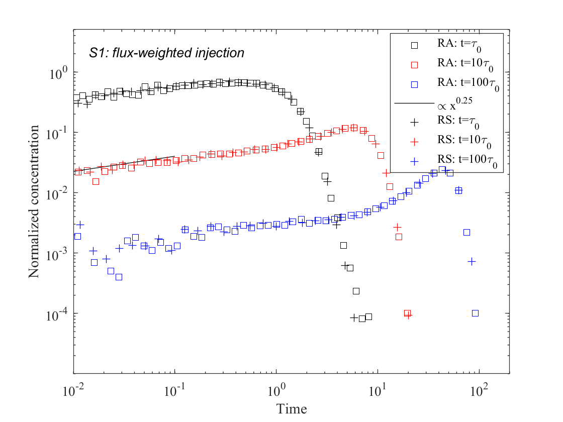
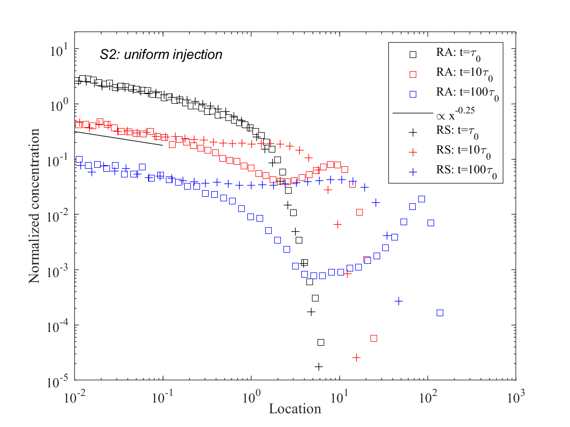
Figure 1: Spatial particle profiles at time (black) $t=\tau_{0}$, (red) $t=10\tau_{0}$ and (blue) $t=100\tau_{0}$ for (top row) scenario S1 ($\gamma=1.25$ and $\alpha=0.25$) under flux-weigthed injection, and (bottom row) scenario S2 ($\gamma=0.75$ and $\alpha=0.75$) under uniform injection. The crosses denote the RS model, the squares the RA model.

III.1.1 Spatial profiles

Figure 1 shows spatial profiles $p(x,t)$ at times $t=\tau_{0},10\tau_{0}$ and $100\tau_{0}$ for the RS and RA models for scenario S1 under flux-weighted and scenario S2 under uniform injection conditions. The profiles for the RS and RA models are indistinguishable in scenario S1. In fact, the two models are identical as shown in Section II.2. The profiles are characterized by a backward tail and a leading edge. For scenario S2, the RS and RA profiles align at short times because the transition time distributions corresponding to the first CTRW step are the same. With increasing time, the peak at the origin erodes in both RS and RA and the behavior close to the origin remain similar. However, the spatial profiles in the RA model develop a second peak at the leading edge that advances much faster than in the RS model. This behavior is due the fact that once particles leave the source zone, they are propagated at higher average velocity in the RA than in the RS model.

III.1.2 Displacement mean and variance

We now focus on the temporal evolutions of the displacement mean and variance for RS and RA in the two scenarios S1 and S2. From CTRW theory (Berkowitz et al., 2006), we expect for the RS model the long-time scalings $m(t)\propto t^{\gamma}$ and $\kappa(t)\propto t^{2\gamma}$ for $0<\gamma<1$ and $m(t)\propto t$ and $\kappa(t)\propto t^{3-\gamma}$. For the RA model, we expect $m(t)\propto t$ and $\kappa(t)\propto t^{2-\alpha}$ for $0<\alpha<1$. These asymptotic behaviors are reflected in the data for the RS and RA models displayed in Figure 2.

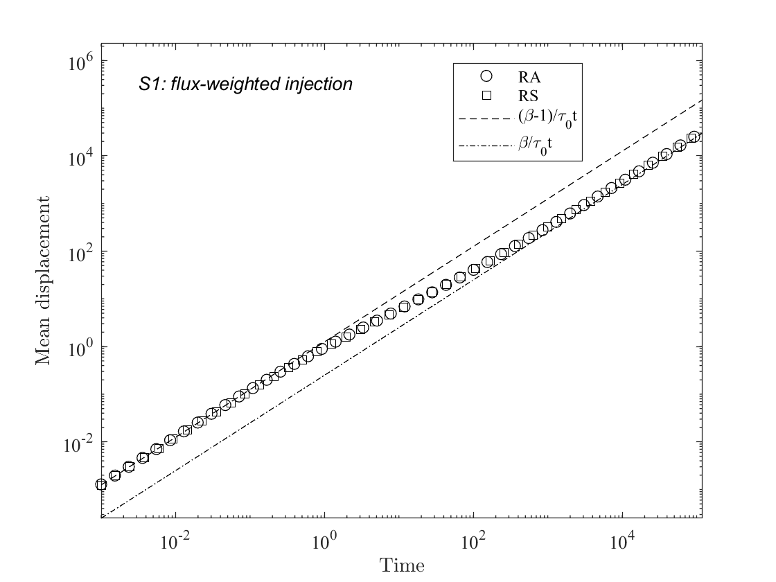
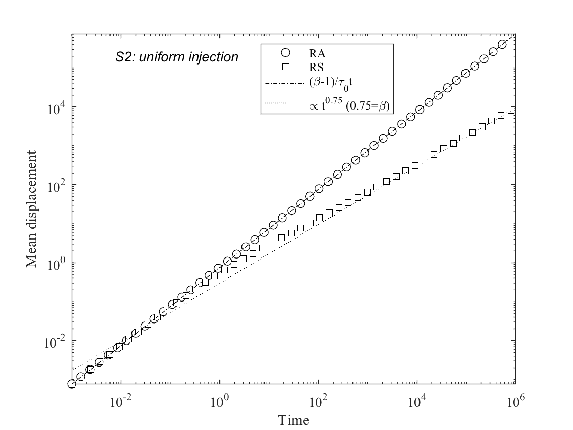
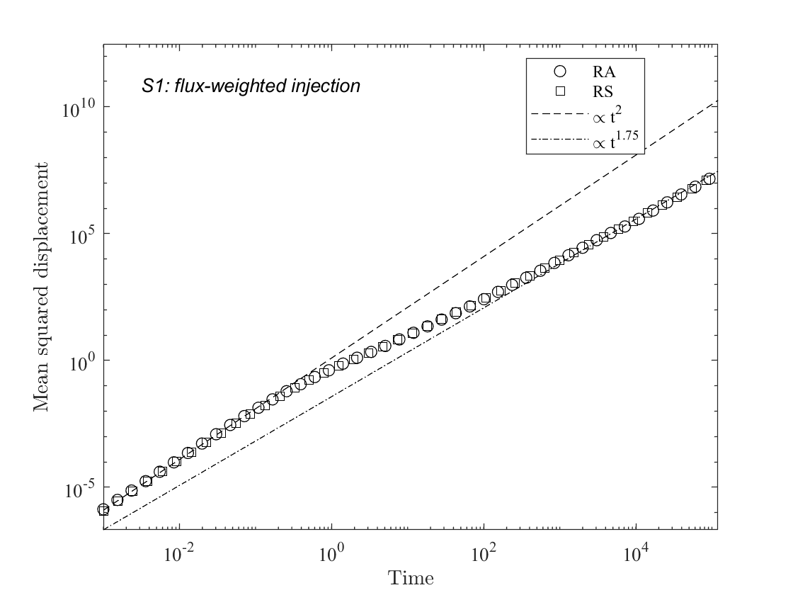
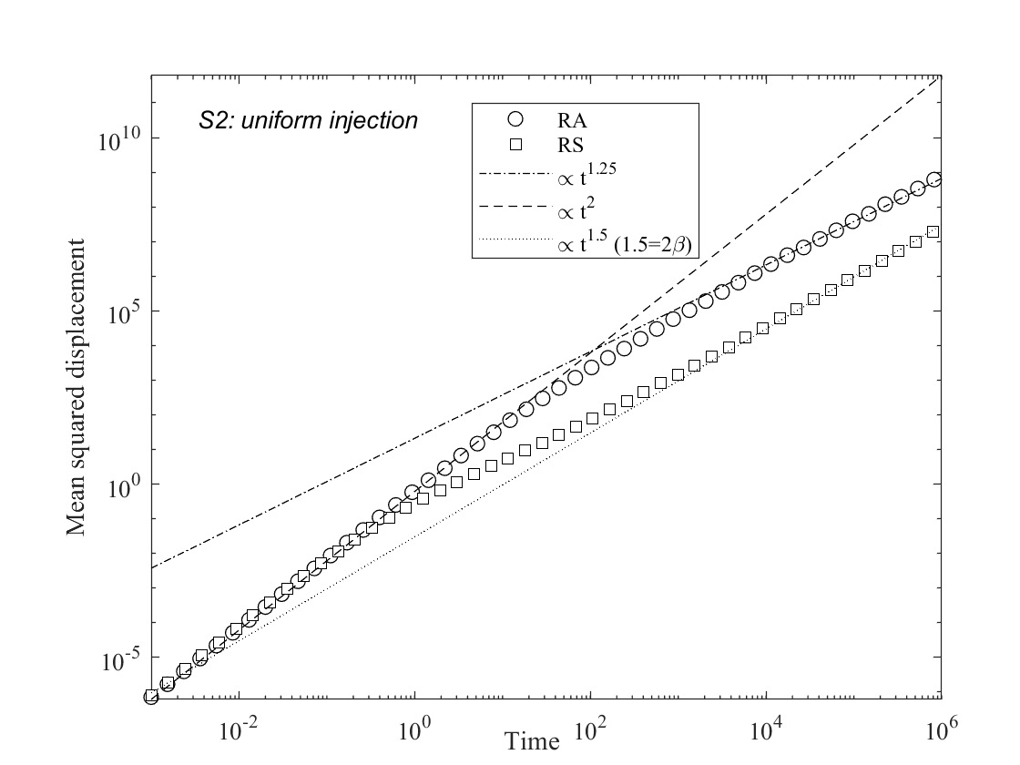
Figure 2: Displacement (top row) mean and (bottom row) variance for (left) scenario S1 ($\gamma=1.25$ and $\alpha=0.25$) under flux-weighted injection, and (right) scenario S2 ($\gamma=0.75$ and $\alpha=0.75$) under uniform injection. The squares denote the RS, the circles denote the RA model.

As shown in the top row of Figure 2, the displacement mean evolves for scenarios initially linearly with time, which reflects the correlation of particle velocities on the scale $\ell_{c}$. The displacement mean for the RS and RA models are identical for flux-weighted injection in S1. The mean displacement evolves linearly in time with two different slopes at early and late times, which is a manifestation of aging, that is, the mean velocity evolves in time (Sokolov, 2012), albeit towards a stationary limit, which is given by the mean flow velocity in the RA model. We call this behavior weak aging because an asymptotic constant velocity exists. The initial velocity is higher than the asymptotic mean due to the flux-weighting in the RA model, while the asymptotic velocity is equal to the mean Eulerian flow velocity. In scenario S2, the mean displacement in the RA and RS models behave in the same way at early times. Here, the RA model does not display aging. Its mean displacement increases linearly with time according to the average flow velocity. The RS model on the other hand, displays aging. Its mean displacement behaves sublinearly as $m(t)\propto t^{3/4}$ due to strong particle retention. We term this behavior here strong aging because there is no asymptotic particle velocity.

As shown in the bottom row of Figure 2, the displacement variances evolve ballistically at early times, that is, according to $\kappa(t)\propto t^{2}$ for the two scenarios. For S1, the behaviors of RS and RA are identical for flux-weighted injection. At large times, $\kappa(t)$ in both models scale as $t^{1.75}$. For scenario S2 the situation is different. While the displacement variances $\kappa(t)$ behave identically for the RS and RA models at short times, at large times, $\kappa(t)\propto t^{3/2}$ for RS and $\propto t^{5/4}$ for RA. The displacement mean and variance in general behave differently in the RA and RS models depending on the initial conditions even though the early or late time scalings may be similar.

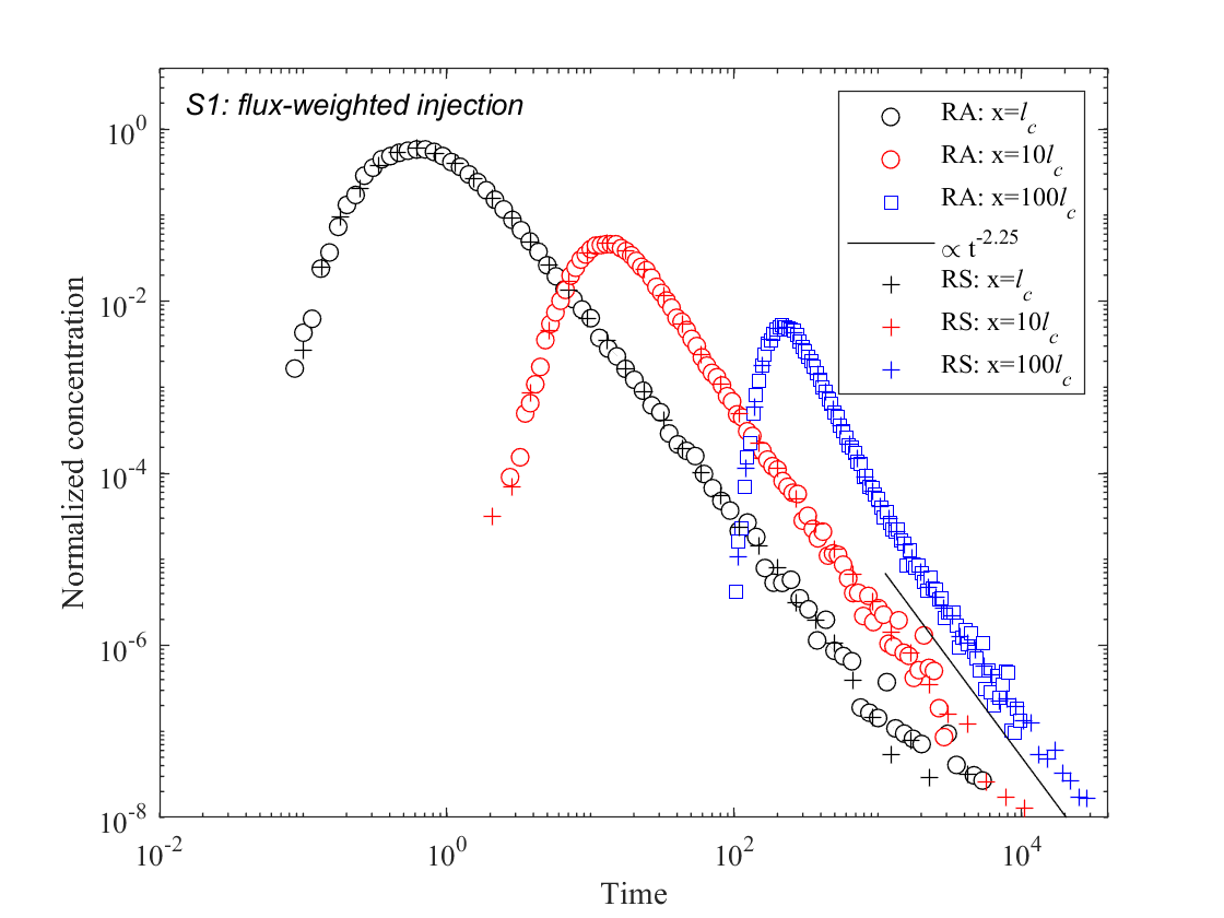
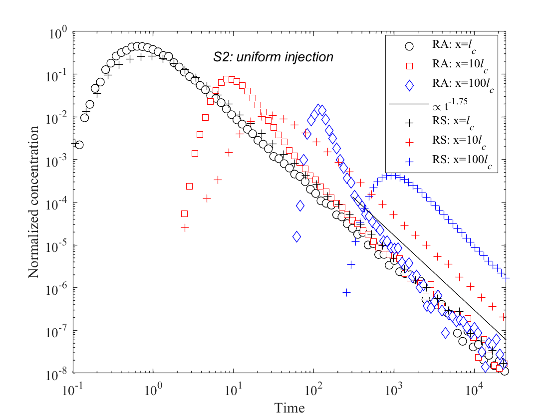
Figure 3: Breakthrough curves for (left) scenario S1 ($\gamma=1.25$ and $\alpha=0.25$) under flux-weigthed injection and (right) scenario S2 ($\gamma=0.75$ and $\alpha=0.75$) under uniform injection. The squares denote the RS, the circles the RA model.

III.1.3 Breakthrough curves

In this section, we consider particle breakthrough curves in scenarios S1 and S2 for the RS and RA models at three different controls planes at distances $\ell_{c}$, $10\ell_{c}$ and $10^{2}\ell_{c}$ from the inlet, see Figure 3. For S1 ($\gamma=\alpha+1$), the breakthrough curves in the RA and RS models are identical as expected. CTRW theory predicts the late time scalings $f(t,x)\propto t^{-1-\gamma}$ for the RS model, and $f(t,x)\propto t^{-2-\alpha}$ for the RA model. For S2 ($\gamma=\alpha$), the breakthrough curves in the RS and RA models have the same late time scalings because the transition time distribution $\psi_{0}(t)\propto t^{-1-\alpha}$ at the inlet scales in the same way as the transition time distribution $\psi(t)\propto t^{-1-\gamma}$ in the RS model. Close to the inlet the breakthrough curves are almost indistinguishable. With increasing distance, however, the peak arrival in the RA model occurs much earlier than in the RS model due to the fast propagation of the bulk of the particle distribution after the initial step. The long-time scaling in the RA model is fully determined by the transition time distribution $\psi_{0}(t)$ for the first CTRW step, while the bulk behavior is determined by $\psi(t)$. This is in contrast to the RS model, for which particle retention is much stronger as expressed in the transition time distribution $\psi(t)\propto t^{-1-\gamma}$. In fact, the generalized central limit theorem implies that the breakathrough curves for the RS model converge towards a one-sided stable law, see also C. Thus, breakthrough curves in the RS and RA models may show similar late time scalings, but the general behaviors are quite different and depend on the injection conditions.

III.2 Transport in the RSA model

We now consider solute transport under the combined impact of heterogeneous sorption and flow velocity. We consider the scenarios S1 and S2 for the distributions of the retardation factor and flow speed defined in Section III.1. That is, we use the Gamma distribution (43) for $p_{e}(v)$ and the inverse Gamma distribution (44) for $p_{R}(r)$. In order to estimate the asymptotic behaviors of the RSA model, we consider the approximation (36) for $\psi(t)$. We find that

$$\psi(t)\propto t^{-1-\beta},$$ (47)

where $\beta=\gamma$ if $\gamma\leq\alpha+1$ and $\beta=\alpha+1$ if $\alpha\leq\gamma-1$, see B. Furthermore, B shows that for uniform injection

$$\psi_{0}(t)\propto t^{-1-\beta_{0}},$$ (48)

where $\beta_{0}=\gamma$ for $\gamma\leq\alpha$ and $\beta_{0}=\alpha$ for $\alpha\leq\gamma$. Under flux-weighted injection, $\beta_{0}=\beta$. We consider in the following scenario S1 under uniform injection and scenario S2 under flux-weigthed injection. Recall that for S1, $\gamma=\alpha+1$ and therefore $\beta=\gamma=\alpha+1$ and $\beta_{0}=\alpha$. For S2, $\gamma=\alpha$, which implies that $\beta=\gamma<\alpha+1$ and $\beta_{0}=\gamma=\alpha$.

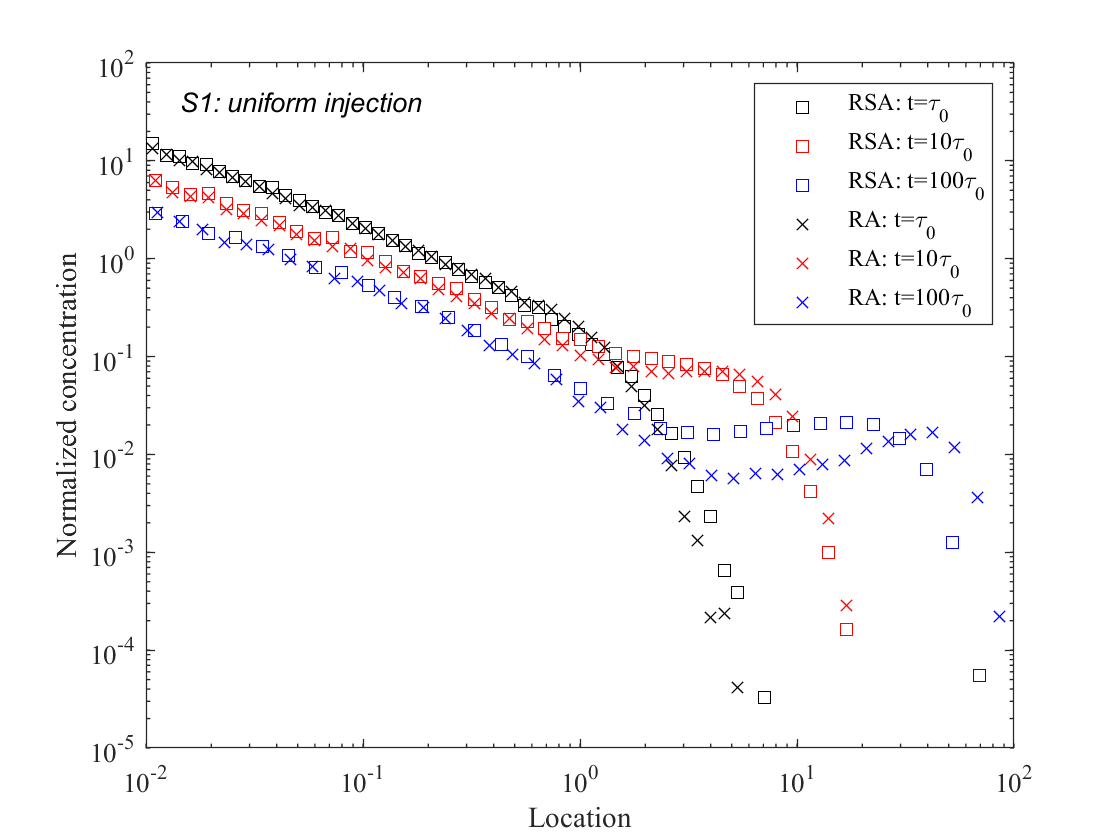
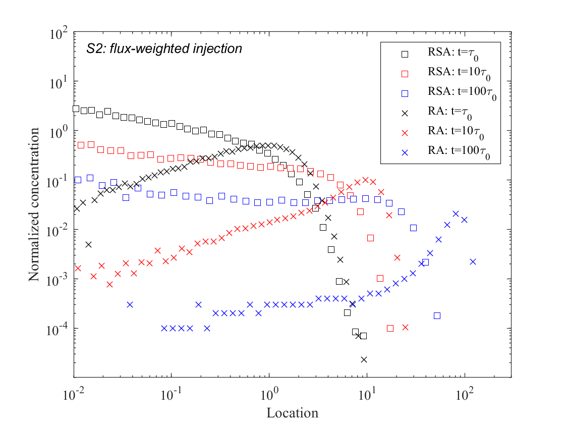
Figure 4: Spatial particle profiles at time (black) $t=\tau_{0}$, (red) $t=10\tau_{0}$ and (blue) $t=100\tau_{0}$ for (left) scenario S1 ($\gamma=1.25$ and $\alpha=0.25$) under uniform injection and (right) scenario S2 ($\gamma=0.75$ and $\alpha=0.75$) under flux-weighted injection.

III.2.1 Spatial profiles

The spatial concentration profiles for the RSA and the corresponding profiles for the RA model are shown in Figure 4. For S1, we observe a strong localization of the peak at the origin due to low velocities in the injection region. The peak erodes and a second peak at the leading edge develops. The profiles behave similarly as in the corresponding RA scenario. The concentration profiles for the RSA model here are dominated by velocity heterogeneity. Variability in the sorption properties manifests in a retardation of the leading edge. Also for S2, we observe peak localization a the origin and the development of a steep leading edge. This behavior, however, is dominated by microscale heterogenity in the sorption properties. The spatial profiles for the RA scenario behave very differently and are characterized by a tailing tail and a peak at the leading edge. While both random sorption and random advection may cause strong retention at the origin, they manifest differently in the behavior of the leading edge.

III.2.2 Displacement mean and variance

Figure 5 shows the displacement mean and variance for S1 under uniform and S2 under flux-weighted injection. For both scenarios, the mean displacement at short times is given by

$$m(t)=\frac{\langle v_{0}\rangle}{R_{H}},$$ (49)

where $\langle v_{0}\rangle$ is the mean initial velocity, and $R_{H}$ the harmonic mean retardation coefficient.

For scenario S1, $\langle v_{0}\rangle=\langle v_{e}\rangle$, which implies that the ratio of the slopes at early and late times gives the ratio of the arithmetic and harmonic mean retardation coefficients. Transport is retarded compared to the corresponding RA model. The long-time behavior of $m(t)$ in scenario S1 is given by

$$m(t)=\frac{\langle v_{e}\rangle}{R_{A}}t,$$ (50)

where $R_{A}$ is the arithmetic mean retardation coefficient.

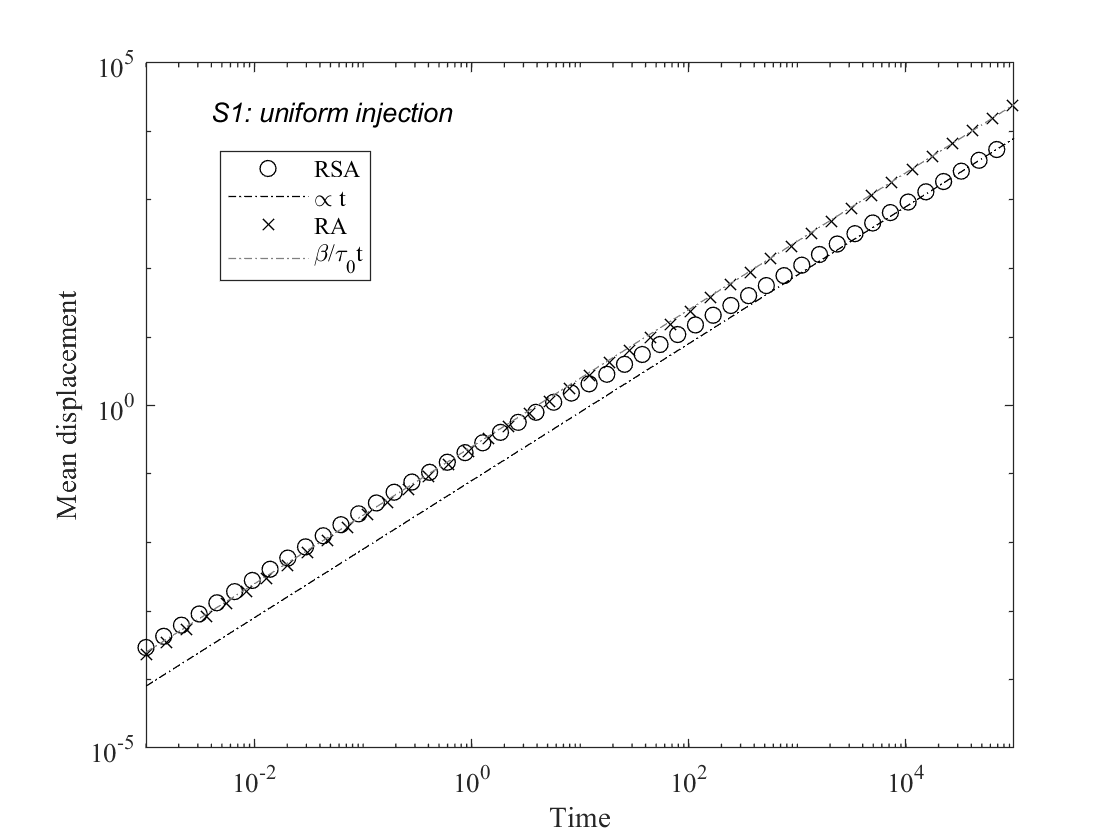
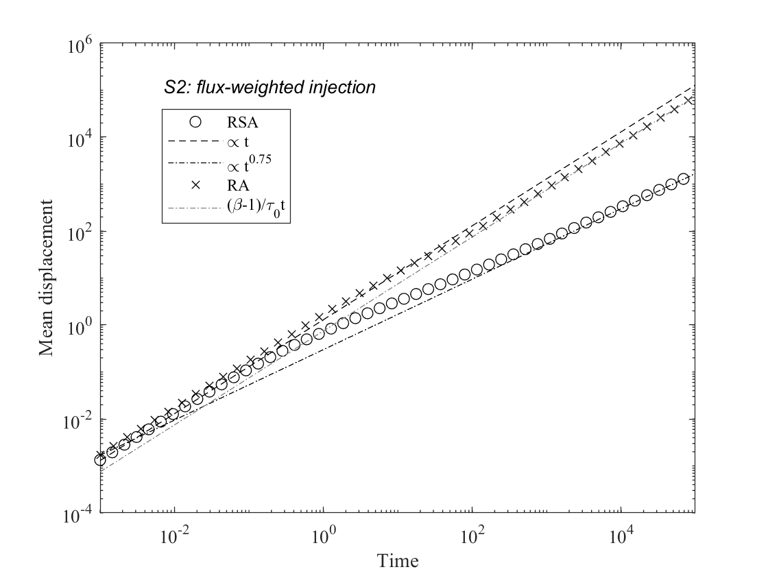
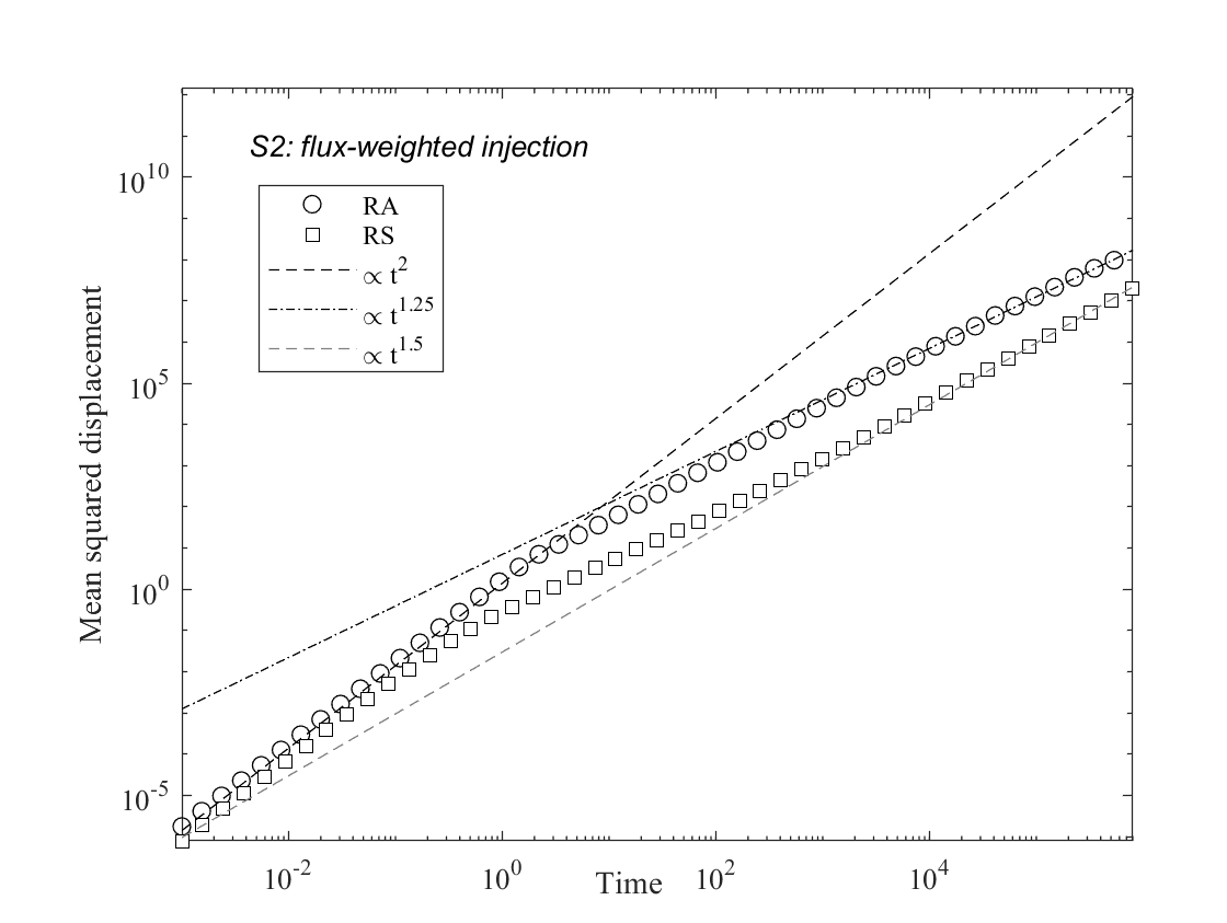
Figure 5: Mean displacements and displacement variance for (left column) scenario S1 ($\gamma=1.25$ and $\alpha=0.25$) under uniform injection and (right column) scenario S2 ($\gamma=0.75$ and $\alpha=0.75$) under flux-weighted injection.

The RSA model displays weak aging, while the mean displacement in the RA model evolves according to the constant mean flow velocity. For scenario S2, the long-time behavior of $m(t)$ scales sublinearly with time according to

$$m(t)\propto t^{\gamma}.$$ (51)

The RSA model is dominated by random sorption and displays strong aging, in contrast to the corresponding RA model.

The displacement variances show at short time the characteristic ballistic behavior, which is given by

$$\sigma^{2}(t)=\left[\sigma_{v_{0}}^{2}\left\langle\mu^{2}\right\rangle+\langle v_{0}\rangle^{2}\sigma_{\mu}^{2}\right]t^{2},$$ (52)

where we defined $\mu=1/R$, and $\sigma_{\mu}^{2}$ is the variance of $\mu$. The long-time scalings are super-linear for both scenarios. Nevertheless, for S1, the long-time behavior is dominated by microscale advection and the scaling is $\sigma^{2}(t)\propto t^{2-\alpha}$. The evolution is delayed due to the presence of random sorption compared to the corresponding RA model. For scenario S2 the behavior is dominated by microscale retardation and the variance scales as $\sigma^{2}(t)\propto t^{2\gamma}$.

III.2.3 Breakthrough curves

Figure 6 shows the breakthrough for S1 under uniform and S2 and flux-weighted injection. The microscale disorder gives rise to strong tailing in both scenarios. In S1, the tailing is dominated by low flow velocities at the injection point and thus, the long-time scaling is given by $f(t,x)\propto t^{-1-\alpha}$. The breakthrough curves are similar to the ones for the corresponding RA model, but show a delay in the peak arrival caused by random sorption. For S2, the breakthrough curve is dominated by random sorption. The long-time scaling is $f(t,x)\propto t^{-1-\gamma}$, and very different from the behavior of the corresponding RA model. Nevertheless, from the asymptotic scaling alone it is not possible to distinguish the dominant microscale disorder mechanism.

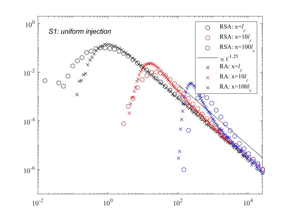
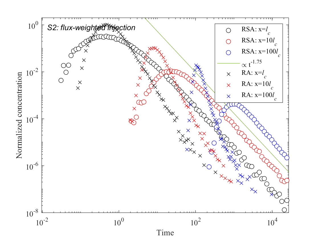
Figure 6: Breakthrough curves for (left) scenario S1 ($\gamma=1.25$ and $\alpha=0.25$) under uniform injection and (bottom row) scenario S2 ($\gamma=0.75$ and $\alpha=0.75$) under flux-weighted injection.

IV Conclusion

In this paper, three CTRW models are derived and their behaviors are studied to explore the impact of random sorption (RS), random advection (RA), and the combination of these two microscale disorder mechanisms (RSA) on large-scale non-Fickian transport. The RS model accounts for instantaneous mobile-immobile mass exchange, which is characterized by a spatially variable retardation coefficient. The RA model quantifies particle transport in media characterized by spatially variable steady flow. The RSA model combines the two microscale disorder models and represents transport in a heterogeneous flow field under instantaneous heterogeneous sorption-desorption. We analyze and compare the transport behaviors in the three models for uniform and flux-weighted initial conditions in terms of spatial profiles of the particle density, the displacement mean and variance, and particle breakthrough curves. In order to probe the impact of the microscale physics on large-scale dispersion, we consider disorder distributions that give the same power-law transition time distributions in the corresponding CTRW models. Under these conditions, the different microscopic disorder models lead to similar large-scale dispersion behaviors. The RA and RS models differ in their responses to initial particle distributions that are not flux-weighted. While the RS model displays always aging for exponents $0<\gamma<1$, Sokolov (2012), that is, the particle velocity is a non-stationary stochastic process, the RA model is stationary for uniform injection conditions, and evolves toward a stationary limit for arbitray initial particle distributions.

The large-scale dispersion signatures in the three disorder models are similar in that they can lead to foward and backward tails in the spatial particle profiles, superdiffusive growth of the displacement variance, and power-law tails in the particle breakthrough curves. However, while the RA model leads always to superdiffusive behavior, the RS model displays subdiffusive behavior for exponents $0<\gamma<1/2$ together with a sublinear scaling of the mean displacement. The spatial profiles can develop double peak behaviors in all models, depending on the microscale disorder distribution for the RS model, and on the injection condition for the RA model. These behaviors are characterized by a localized peak at the origin that erodes with time, and a peak at the leading front. The RA model does not display double peak behavior for flux-weighted injection, but gives a trailing tail and well-defined peak at the front, similar to the RS model for $1<\gamma<2$. Under uniform injection, the RA model develops two clearly separated peaks and a fast moving leading edge. The breakthrough curves display power-law scaling $\propto t^{-1-\beta}$ with $0<\beta<2$ for all disorder models. The power-law range $0<\beta<1$ corresponds in the RS model to the exponents $0<\gamma<1$. In this case, the breakthrough curve converges toward a one-sided stable distribution. In the RA model, in contrast, this behavior can only be observed for uniform injection, and the breakthrough curve does not converge to a stable distribution. In this case, the tail behavior is fully determined by the transition time distribution for the first CTRW step, and the peak arrival is much earlier than in the RS model with the same tailing behavior.

In conclusion, while the large-scale signatures of dispersion in the disorder models under consideration are similar, their responses to initial particle distributions that are not flux-weighted can be very different. Thus, under certain conditions, it is possible to infer the microscale physics from the observation of the dispersion behavior. A CTRW model with power-law transition time distribution in general allows to reproduce anomalous dispersion as manifest in non-linear scalings of displacement mean and variance, and power-law tails in particle breakthrough curve. However, it is important to identify and characterize the microscale physics and disorder properties to be able to predict the large scale system behaviors.

Appendix A Boltzmann equation for the RSA model

The joint distribution $p(x,v,r,t)$ of particle position, velocity and retardation coefficient can be written as

$$p(x,v,r,t) =\frac{r}{v}\int\limits_{0}^{\infty}ds\langle\delta[x-x(s)]\delta[v-v(s)]\delta[r-R(s)]\delta[t-t(s)]\rangle$$ (53)

$$=\frac{r}{v}\int\limits_{0}^{\infty}dsR(x,v,r,t,s)$$ (54)

The derivative of $R(x,v,r,t,s)$ along $s$ is given by particle conservation as

$$\frac{\partial R(x,v,r,t,s)}{\partial s} =-\frac{\partial R(x,v,r,t,s)}{\partial x}+\frac{D}{v}\frac{\partial^{2}R(x,v,r,t,s)}{\partial x^{2}}-\frac{r}{v}\frac{\partial R(x,v,r,t,s)}{\partial t}$$

$$+\frac{1}{\ell_{c}}\int\limits_{0}^{\infty}dv^{\prime}\int\limits_{0}^{\infty}dr^{\prime}p_{v}(v)\psi_{R}(r)R(x,v^{\prime},r^{\prime},t,s)-\frac{1}{\ell_{c}}R(x,v,r,t,s)$$ (55)

Integration of the latter over $s$ according to Eq. (54) gives Eq. (33).

Appendix B Scaling of transition time distribution for the RSA model

The transition time distribution of the RSA model can be written as

$$\psi(t)=\int_{0}^{\infty}{dr}\int_{0}^{\infty}{dv\delta\left({t-\frac{{\ell_{c}r}}{v}}\right){p_{R}}\left(r\right){p_{v}}\left(v\right)},$$ (56)

where $\delta(x)$ denotes the Dirac Delta. Using that $\delta(ax)=\frac{1}{|a|}\delta(x)$, we obtain Eq. (36). We use expression (44) for $p_{R}(r)$ and for $p_{v}(v)$, we use expression (43) for $p_{e}(v)$ in definition (19) for $p_{v}(v)$ to obtain

$$p_{v}(v)=\left(\frac{v}{v_{0}}\right)^{\alpha}\frac{\exp(-v/v_{0})}{v_{0}\Gamma(\alpha+1)}$$ (57)

Using these expressions in Eq. (36) we obtain

$$\psi(t)=\int_{0}^{\infty}{dv\frac{v}{\ell_{c}}{{\left({\frac{{vt}}{{\ell_{c}{r_{0}}}}}\right)}^{-\gamma-1}}}\frac{e^{-\frac{{\ell_{c}{r_{0}}}}{{vt}}}}{r_{0}\Gamma(\gamma)}{\left({\frac{v}{{{v_{0}}}}}\right)^{\alpha}}\frac{e^{-\frac{v}{{{v_{0}}}}}}{{{v_{0}}\Gamma\left(\alpha+1\right)}},$$ (58)

For $\gamma<\alpha+1$ and $t\gg\ell_{c}r_{0}/v_{0}$, Eq. (58) can be approximated as

$$\psi(t)=\left(\frac{v_{0}t}{\ell_{c}r_{0}}\right)^{-1-\gamma}\frac{v_{0}}{\ell_{c}r_{0}}\int_{0}^{\infty}dv\left(\frac{v}{v_{0}}\right)^{\alpha-\gamma}{\frac{{e^{-\frac{v}{v_{0}}}}}{\Gamma(\gamma)\Gamma(\alpha+1)v_{0}}},$$ (59)

where we used that ${e^{-{\ell_{c}r_{0}\over{vt}}}}\to 1$ for $t\gg\ell_{c}r_{0}/v_{0}$. Evaluating the integral on the right side, we obtain

$$\psi(t)=\left(\frac{v_{0}t}{\ell_{c}r_{0}}\right)^{-1-\gamma}\frac{v_{0}}{\ell_{c}r_{0}}\frac{\Gamma(\alpha-\gamma+1)}{\Gamma(\gamma)\Gamma(\alpha+1)},$$ (60)

For $\alpha<\gamma-1$, we perform the variable transform $v\to\ell=vt/r_{0}$ in (58), which gives

$$\psi(t)=\left(\frac{v_{0}t}{\ell_{c}r_{0}}\right)^{-\alpha-2}\frac{v_{0}}{\ell_{c}r_{0}}\int_{0}^{\infty}d\ell\left(\frac{\ell}{\ell_{c}}\right)^{-(\gamma-\alpha-1)-1}\frac{e^{-\frac{\ell_{c}}{\ell}}}{\Gamma(\gamma)}\frac{e^{-\frac{\ell r_{0}}{v_{0}t}}}{\Gamma\left(\alpha+1\right)}.$$ (61)

In the limit $t\gg\ell_{c}r_{0}/v_{0}$, the integral on the right side can be evaluated explicitly, which gives

$$\psi(t)=\left(\frac{v_{0}t}{\ell_{c}r_{0}}\right)^{-\alpha-2}\frac{v_{0}}{\ell_{c}r_{0}}\frac{\Gamma(\gamma-\alpha-1)}{\Gamma(\gamma)\Gamma\left(\alpha+1\right)}.$$ (62)

For $\psi_{0}(t)$ in the case of uniform injection, the derivations are analogous. For $\gamma<\alpha$, we obtain

$$\psi_{0}(t)=\left(\frac{v_{0}t}{\ell_{c}r_{0}}\right)^{-1-\gamma}\frac{v_{0}}{\ell_{c}r_{0}}\frac{\Gamma(\alpha-\gamma)}{\Gamma(\gamma)\Gamma(\alpha)},$$ (63)

For $\alpha<\gamma$, we obtain

$$\psi_{0}(t)=\left(\frac{v_{0}t}{\ell_{c}r_{0}}\right)^{-\alpha-1}\frac{v_{0}}{\ell_{c}r_{0}}\frac{\Gamma(\gamma-\alpha)}{\Gamma(\gamma)\Gamma\left(\alpha\right)}.$$ (64)

Appendix C One-sided stable distribution in the RS model

We discuss the convergence of the particle breakthrough curves toward a one-sided stable law with distance of the control plane in the RS model. To this end, we consider the particle arrival time in the corresponding CTRW model (9) for the constant transition length $\xi=\ell_{c}$. Thus, the arrival $t_{n}$ at a control plane at distance $x_{n}=n\ell_{c}$ from the inlet is

$$t_{n}=\sum\limits_{n=1}^{n}\tau_{n},$$ (65)

where the transition times $\tau_{n}$ are distributed according to the heavy-tailed $\psi(t)\propto t^{-1-\gamma}$ for $0<\gamma<1$. According to the generalized central limit theory, the distribution $t_{n}$ converges toward a one-sided stable distribution Uchaikin and Zolotarev (1999).

References

- Adams and Gelhar (1992) Adams, E.E., Gelhar, L.W., 1992. Field study of disperion in a heterogeneous aquifer 2. spatial moment analysis. Water Resour. Res. 28, 3293–3307.
- Aquino and Velásquez-Parra (2022) Aquino, T., Velásquez-Parra, A., 2022. Impact of velocity correlations on longitudinal dispersion in space-lagrangian advective transport models. Physical Review Fluids 7, 024501.
- Becker and Shapiro (2003) Becker, M.W., Shapiro, A.M., 2003. Interpreting tracer breakthrough tailing from different forced-gradient tracer experiment configurations in fractured bedrock. Water Resour. Res. 39.
- Benson and Meerschaert (2009) Benson, D.A., Meerschaert, M.M., 2009. A simple and efficient random walk solution of multi-rate mobile/immobile mass transport equations. Advances in Water Resources 32, 532–539.
- Benson et al. (2001) Benson, D.A., Schumer, R., Meerschaert, M.M., Wheatcraft, S.W., 2001. Fractional dispersion, lévy motion, and the made tracer tests. Transport in porous media 42, 211–240.
- Berkowitz et al. (2006) Berkowitz, B., Cortis, A., Dentz, M., Scher, H., 2006. Modeling non-fickian transport in geological formations as a continuous time random walk. Reviews of Geophysics 44.
- Bijeljic et al. (2011) Bijeljic, B., Mostaghimi, P., Blunt, M.J., 2011. Signature of non-Fickian solute transport in complex heterogeneous porous media 107, 204502.
- Carrera et al. (1998) Carrera, J., Sánchez-Vila, X., Benet, I., Medina, A., Galarza, G.A., Guimerá, J., 1998. On matrix diffusion: formulations, solution methods and qualitative effects. Hydrogeol. J. 6, 178–190.
- Coats and Smith (1964) Coats, K., Smith, B., 1964. Dead-end pore volume and dispersion in porous media. Society of petroleum engineers journal 4, 73–84.
- Comolli et al. (2019) Comolli, A., Hakoun, V., Dentz, M., 2019. Mechanisms, upscaling, and prediction of anomalous dispersion in heterogeneous porous media. Water Resources Research 55, 8197–8222.
- Cushman and Ginn (2000) Cushman, J.H., Ginn, T.R., 2000. Fractional advection-dispersion equation: A classical mass balance with convolution-fickian flux. Water resources research 36, 3763–3766.
- Cvetkovic et al. (2014) Cvetkovic, V., Fiori, A., Dagan, G., 2014. Solute transport in aquifers of arbitrary variability: A time-domain random walk formulation. Water Resources Research 50, 5759–5773.
- De Anna et al. (2013) De Anna, P., Le Borgne, T., Dentz, M., Tartakovsky, A.M., Bolster, D., Davy, P., 2013. Flow intermittency, dispersion, and correlated continuous time random walks in porous media. Physical Review Letters 110, 184502.
- Delay and Bodin (2001) Delay, F., Bodin, J., 2001. Time domain random walk method to simulate transport by advection-dispersion and matrix diffusion in fracture networks. Geophysical Research Letters 28, 4051–4054.
- Demmy et al. (1999) Demmy, G., Berglund, S., Graham, W., 1999. Injection mode implications for solute transport in porous media: Analysis in a stochastic lagrangian framework. Water resources research 35, 1965–1973.
- Dentz and Berkowitz (2003) Dentz, M., Berkowitz, B., 2003. Transport behavior of a passive solute in continuous time random walks and multirate mass transfer. Water Resources Research 39.
- Dentz and Bolster (2010) Dentz, M., Bolster, D., 2010. Distribution-versus correlation-induced anomalous transport in quenched random velocity fields. Physical review letters 105, 244301.
- Dentz and Castro (2009) Dentz, M., Castro, A., 2009. Effective transport dynamics in porous media with heterogeneous retardation properties. Geophysical Research Letters 36.
- Dentz et al. (2004) Dentz, M., Cortis, A., Scher, H., Berkowitz, B., 2004. Time behavior of solute transport in heterogeneous media: transition from anomalous to normal transport. Advances in Water Resources 27, 155–173.
- Dentz et al. (2016) Dentz, M., Kang, P.K., Comolli, A., Le Borgne, T., Lester, D.R., 2016. Continuous time random walks for the evolution of lagrangian velocities. Physical Review Fluids 1, 074004.
- Frippiat and Holeyman (2008) Frippiat, C.C., Holeyman, A.E., 2008. A comparative review of upscaling methods for solute transport in heterogeneous porous media. Journal of Hydrology 362, 150–176.
- Gouze et al. (2008) Gouze, P., Melean, Y., Le Borgne, T., Dentz, M., Carrera, J., 2008. Non-fickian dispersion in porous media explained by heterogeneous microscale matrix diffusion. Water Resources Research 44. doi:10.1029/2007WR006690.
- Green (2000) Green, C., 2000. Connected-network paradigm for the alluvial aquifer system. Theory, Modeling, and Field Investigation in Hydrogeology: A Special Volume in Honor of Shlomo P. Neuman’s 60th Birthday 348, 25.
- Haggerty et al. (2001) Haggerty, R., Fleming, S.W., Meigs, L.C., McKenna, S.A., 2001. Tracer tests in a fractured dolomite: 2. analysis of mass transfer in single-well injection-withdrawal tests. Water Resources Research 37, 1129–1142.
- Haggerty and Gorelick (1995) Haggerty, R., Gorelick, S.M., 1995. Multiple-rate mass transfer for modeling diffusion and surface reactions in media with pore-scale heterogeneity. Water Resources Research 31, 2383–2400.
- Han et al. (2021) Han, X., Zhang, Y., Zheng, C., Yu, X., Li, S., Wei, W., 2021. Enhanced cr (vi) removal from water using a green synthesized nanocrystalline chlorapatite: Physicochemical interpretations and fixed-bed column mathematical model study. Chemosphere 264, 128421.
- Harvey and Gorelick (2000) Harvey, C., Gorelick, S.M., 2000. Rate-limited mass transfer or macrodispersion: Which dominates plume evolution at the macrodispersion experiment (made) site? Water Resources Research 36, 637–650.
- Hidalgo et al. (2021) Hidalgo, J.J., Neuweiler, I., Dentz, M., 2021. Transport under advective trapping. Journal of Fluid Mechanics 907, A36.
- Hyman et al. (2015) Hyman, J., Painter, S.L., Viswanathan, H., Makedonska, N., Karra, S., 2015. Influence of injection mode on transport properties in kilometer-scale three-dimensional discrete fracture networks. Water Resources Research 51, 7289–7308.
- Hyman and Dentz (2021) Hyman, J.D., Dentz, M., 2021. Transport upscaling under flow heterogeneity and matrix-diffusion in three-dimensional discrete fracture networks. Advances in Water Resources 155, 103994.
- Janković and Fiori (2010) Janković, I., Fiori, A., 2010. Analysis of the impact of injection mode in transport through strongly heterogeneous aquifers. Advances in Water Resources 33, 1199–1205.
- Kang et al. (2014) Kang, P.K., de Anna, P., Nunes, J., Bijeljic, B., Blunt, M.J., Juanes, R., 2014. Pore-scale intermittent velocity structure underpinning anomalous transport through 3-d porous media. Geophys. Res. Lett. 41 (17), 6184–6190.
- Kang et al. (2017) Kang, P.K., Dentz, M., Le Borgne, T., Lee, S., Juanes, R., 2017. Anomalous transport in disordered fracture networks: Spatial markov model for dispersion with variable injection modes. Advances in Water Resources 106, 80–94.
- Kang et al. (2015) Kang, P.K., Le Borgne, T., Dentz, M., Bour, O., Juanes, R., 2015. Impact of velocity correlation and distribution on transport in fractured media: Field evidence and theoretical model. Water Resources Research 51, 940–959.
- Kilbas et al. (2006) Kilbas, A.A., Srivastava, H.M., Trujillo, J.J., 2006. Theory and applications of fractional differential equations. volume 204. elsevier.
- Le Borgne et al. (2008) Le Borgne, T., Dentz, M., Carrera, J., 2008. A lagrangian statistical model for transport in highly heterogeneous velocity fields. Phys. Rev. Lett. 101, 090601.
- Liu and Kitanidis (2012) Liu, Y., Kitanidis, P.K., 2012. Applicability of the dual-domain model to nonaggregated porous media. Groundwater 50, 927–934.
- Lu et al. (2018) Lu, B., Song, J., Li, S., Tick, G.R., Wei, W., Zhu, J., Zheng, C., Zhang, Y., 2018. Quantifying transport of arsenic in both natural soils and relatively homogeneous porous media using stochastic models. Soil Science Society of America Journal 82, 1057–1070.
- Meerschaert and Sikorskii (2019) Meerschaert, M.M., Sikorskii, A., 2019. Stochastic models for fractional calculus. volume 43. Walter de Gruyter GmbH & Co KG.
- Morales et al. (2017) Morales, V.L., Dentz, M., Willmann, M., Holzner, M., 2017. Stochastic dynamics of intermittent pore-scale particle motion in three-dimensional porous media: Experiments and theory. Geophysical Research Letters 44, 9361–9371.
- Neuman and Tartakovsky (2009) Neuman, S.P., Tartakovsky, D.M., 2009. Perspective on theories of non-fickian transport in heterogeneous media. Advances in Water Resources 32, 670–680.
- Nkedi-Kizza et al. (1985) Nkedi-Kizza, P., Rao, P.S.C., Hornsby, A.G., 1985. Influence of organic cosolvents on sorption of hydrophobic organic chemicals by soils. Environmental science & technology 19, 975–979.
- Noetinger et al. (2016) Noetinger, B., Roubinet, D., Russian, A., Le Borgne, T., Delay, F., Dentz, M., De Dreuzy, J.R., Gouze, P., 2016. Random walk methods for modeling hydrodynamic transport in porous and fractured media from pore to reservoir scale. Transport in Porous Media 115, 345–385.
- Painter et al. (2008) Painter, S., Cvetkovic, V., Mancillas, J., Pensado, O., 2008. Time domain particle tracking methods for simulating transport with retention and first-order transformation. Water resources research 44.
- Puyguiraud et al. (2019) Puyguiraud, A., Gouze, P., Dentz, M., 2019. Upscaling of anomalous pore-scale dispersion. Transport in Porous Media 128, 837–855. URL: https://doi.org/10.1007/s11242-019-01273-3, doi:10.1007/s11242-019-01273-3.
- Schumer et al. (2003) Schumer, R., Benson, D.A., Meerschaert, M.M., Baeumer, B., 2003. Fractal mobile/immobile solute transport. Water Resources Research 39.
- Sherman et al. (2021) Sherman, T., Engdahl, N.B., Porta, G., Bolster, D., 2021. A review of spatial markov models for predicting pre-asymptotic and anomalous transport in porous and fractured media. Journal of Contaminant Hydrology 236, 103734.
- Sokolov (2012) Sokolov, I.M., 2012. Models of anomalous diffusion in crowded environments. Soft Matter 8, 9043–9052.
- Sun et al. (2015) Sun, H., Chen, D., Zhang, Y., Chen, L., 2015. Understanding partial bed-load transport: Experiments and stochastic model analysis. Journal of Hydrology 521, 196–204.
- Sun et al. (2020) Sun, L., Qiu, H., Wu, C., Niu, J., Hu, B.X., 2020. A review of applications of fractional advection–dispersion equations for anomalous solute transport in surface and subsurface water. WIREs Water 7. URL: https://doi.org/10.1002/wat2.1448, doi:10.1002/wat2.1448.
- Uchaikin and Zolotarev (1999) Uchaikin, V.V., Zolotarev, V.M., 1999. Chance and stability: stable distributions and their applications. Walter de Gruyter.
- Willmann et al. (2008) Willmann, M., Carrera, J., Sánchez-Vila, X., 2008. Transport upscaling in heterogeneous aquifers: What physical parameters control memory functions? Water Resources Research 44. URL: https://doi.org/10.1029/2007wr006531, doi:10.1029/2007wr006531.
- Yoon and Kang (2021) Yoon, S., Kang, P.K., 2021. Roughness, inertia, and diffusion effects on anomalous transport in rough channel flows. Physical Review Fluids 6, 014502.
- Zhang et al. (2005) Zhang, X., Crawford, J.W., Deeks, L.K., Stutter, M.I., Bengough, A.G., Young, I.M., 2005. A mass balance based numerical method for the fractional advection-dispersion equation: Theory and application. Water resources research 41.
- Zhang et al. (2013) Zhang, Y., Green, C.T., Fogg, G.E., 2013. The impact of medium architecture of alluvial settings on non-fickian transport. Advances in Water Resources 54, 78–99. URL: https://doi.org/10.1016/j.advwatres.2013.01.004, doi:10.1016/j.advwatres.2013.01.004.
- Zhang et al. (2015) Zhang, Y., Meerschaert, M.M., Baeumer, B., LaBolle, E.M., 2015. Modeling mixed retention and early arrivals in multidimensional heterogeneous media using an explicit lagrangian scheme. Water Resources Research 51, 6311–6337.
- Zhang et al. (2019) Zhang, Y., Yu, X., Li, X., Kelly, J.F., Sun, H., Zheng, C., 2019. Impact of absorbing and reflective boundaries on fractional derivative models: Quantification, evaluation and application. Advances in Water Resources 128, 129–144.
- Zheng and Gorelick (2003) Zheng, C., Gorelick, S.M., 2003. Analysis of solute transport in flow fields influenced by preferential flowpaths at the decimeter scale. Groundwater 41, 142–155.