Photometry and astrometry with JWST – III. A NIRCam-Gaia DR3 analysis of the open cluster NGC 2506

Abstract

In the third paper of this series aimed at developing the tools for analysing resolved stellar populations using the cameras on board of the James Webb Space Telescope (JWST), we present a detailed multi-band study of the 2 Gyr Galactic open cluster NGC 2506. We employ public calibration data-sets collected in multiple filters to: (i) derive improved effective Point Spread Functions (ePSFs) for ten NIRCam filters; (ii) extract high-precision photometry and astrometry for stars in the cluster, approaching the main-sequence (MS) lower mass of $\sim 0.1~{}M_{\odot}$; and (iii) take advantage of the synergy between JWST and Gaia DR3 to perform a comprehensive analysis of the cluster’s global and local properties. We derived a MS binary fraction of $\sim$57.5 %, extending the Gaia limit ($\sim 0.8~{}M_{\odot}$) to lower masses ($\sim 0.4~{}M_{\odot}$) with JWST. We conducted a study on the mass functions (MFs) of NGC 2506, mapping the mass segregation with Gaia data, and extending MFs to lower masses with the JWST field. We also combined information on the derived MFs to infer an estimate of the cluster present-day total mass. Lastly, we investigated the presence of white dwarfs (WDs) and identified a strong candidate. However, to firmly establish its cluster membership, as well as that of four other WD candidates and of the majority of faint low-mass MS stars, further JWST equally deep observations will be required. We make publicly available catalogues, atlases, and the improved ePSFs.

1 Introduction

When we observe a Galactic stellar cluster, whether it is open or globular, it is like looking at a snapshot of stars with different masses but approximately the same initial chemical composition, age, and distance. By studying stellar clusters with varying chemical compositions and ages ranging from a few tens of Myr up to $\sim 10$–13 Gyr, we can gain insights into the processes involved in the formation and evolution of stars with different mass and metallicity. Optical and UV studies using data from the Hubble Space Telescope (HST) have led to the discovery of several phenomena that were previously unknown, such as, for example, the existence of multiple stellar populations in globular clusters (see, e.g., Bedin et al. 2004; Piotto et al. 2007, 2015), and the unusual shape of some stellar clusters’ white dwarf cooling sequences (e.g., Bedin et al. 2008; Bellini et al. 2013). However, with few exceptions (see, e.g., King et al. 2005; Richer et al. 2008; Dieball et al. 2016), observations of open and globular clusters have been primarily focused on main-sequence (MS) stars with masses $\gtrsim 0.1~{}M_{\odot}$, and it has been challenging to study stars near the hydrogen burning limit (HBL) and the brown dwarf sequence. In this regard, infrared (IR) photometry plays a crucial role in providing information about low-mass (pre-)MS stars ($M\lesssim$0.1–0.2 $M_{\odot}$) and brown dwarfs in stellar clusters (Nardiello et al. 2023).

Since July 2022, the James Webb Space Telescope (JWST, Gardner et al. 2023) has been acquiring a vast amount of IR data through its cameras, revolutionising our understanding of the Universe. Public Director’s Discretionary-Early Release Science (DD-ERS) and Calibration JWST data constitute a treasure for improving data reduction techniques and at the same time yield scientifically significant results (see, e.g., Nardiello et al. 2022, hereafter Paper I and II, respectively; Griggio et al. 2023b, hereafter Paper I and II, respectively). Currently, non-proprietary data in the archive encompass observations of high-redshift galaxies (e.g., Naidu et al. 2022) and galaxy clusters (e.g., Paris et al. 2023), resolved close dwarf galaxies and portions of the Large Magellanic Cloud (LMC, e.g., Paper II; Libralato et al. 2023), Galactic stellar clusters (e.g., Paper I; Ziliotto et al. 2023), individual stars and exoplanets (e.g., Feinstein et al. 2023), and objects of the Solar System (e.g., de Pater et al. 2022).

In this study, we took advantage of the publicly available calibration observations to conduct an IR multi-band investigation of the lower MS stars in the open cluster NGC 2506. The data were collected with the JWST Near Infrared Camera (NIRCam, Rieke et al. 2023) as part of the calibration programme CAL-1538 (PI: Gordon). The primary objective of this programme is to acquire observations of G dwarf stars for the flux calibration of JWST filters. Additionally, we utilised data from the CAL-1476 programme (PI: Boyer) targeting stars in the LMC to derive effective Point Spread Functions for nearly all available NIRCam filters, spanning a wavelength range from $\sim 0.7~{}\mu$m to $\sim 4.5~{}\mu$m.

The open cluster NGC 2506 is particularly interesting since it belongs to the (small) sample of metal-poor ([Fe/H]$\lesssim-0.1$), old-age ($\gtrsim 1$ Gyr) open clusters located at the Galactic anti-centre, at $\sim 3$ kpc from the Sun (McClure et al. 1981; Cantat-Gaudin & Anders 2020); similar clusters in this category include NGC 2420 and NGC 2243 (Anthony-Twarog et al. 2005, 2006). NGC 2506 has been the subject of several studies to determine its age and metallicity (Carretta et al. 2004; Mikolaitis et al. 2011; Anthony-Twarog et al. 2016; Knudstrup et al. 2020), analyse the evolution of surface lithium abundances (Anthony-Twarog et al. 2018), investigate its structural parameters (Lee et al. 2013; Rangwal et al. 2019; Gao 2020), and identify binary systems and blue straggler stars (Arentoft et al. 2007; Panthi et al. 2022). There have been some discrepancies among these studies regarding the age and metallicity of the cluster members, although all analyses provide an age range between 1 and 3 Gyr and classify the cluster members as highly metal-deficient, with an upper limit of [Fe/H] around $-0.2$ (Netopil et al. 2016). From a dynamical perspective, NGC 2506 is of significant interest. Several studies suggest that the cluster is dynamically relaxed, displaying clear evidence of mass segregation, evaporation of low-mass stars, and even hints of tidal tails (Lee et al. 2013; Rangwal et al. 2019; Gao 2020).

In this work, we investigate all these aspects of this peculiar open cluster, by combining JWST photometry and astrometry with Gaia DR3 (Gaia Collaboration et al. 2021) and ground-based data. Section 2 reports the technical part of this work; it includes a description of the adopted space and ground-based observations, the description of the procedure to derive the effective point spread functions, and the data reduction. Section 3 describes the photometric and astrometric properties of the stars, while Sect. 4 includes the derivation of the radial stellar density profile of the cluster and its structural parameters. Section 5 reports in detail the analysis of the MS binary fraction and of the mass functions extracted from both JWST and Gaia data, while Sect. 6 discusses the candidate white dwarfs we found. A summary is reported in Sect. 7.

2 Observations and data reduction

In this section, we report a description of the JWST data used in this work and the procedures adopted to derive effective point spread functions (ePSFs) and the astro-photometric catalogues of NGC 2506. We also describe how we obtained the catalogues from both ground-based data-sets and selections of the Gaia DR3.

2.1 Large Magellanic cloud JWST data-set

We employed the NIRCam@JWST data of the LMC collected during the Calibration Programme CAL-1476 (PI: Boyer) to derive the ePSFs in 10 different filters. Specifically, we used images collected with the Short Wavelength (SW) channel in F070W, F090W, F115W, F150W, and F200W filters, and with the Long Wavelength (LW) channel in F250M, F277W, F356W, F444W, and F460M filters. As detailed in Paper II, nine pointings are available for each filter. Observations in F277W and F356W filters were conducted using the BRIGHT1 readout pattern and an effective exposure time $t_{\rm exp}=96.631$ s (corresponding to 5 groups of 1 averaged frame). For the F460M filter, the BRIGHT2 readout pattern and $t_{\rm exp}=85.894$ s (4 groups of 2 averaged frames) were employed. Images in all the other filters were taken using the RAPID readout patter, with 2 groups containing 1 frame ( $t_{\rm exp}=21.474$ s). The top panel of Fig. 1 displays the Total System Throughput for each filter.

For our analysis, we utilised the _cal images created by the Stage 2 pipeline calwebb_image2; we converted the value of each pixel from MJy/sr into counts by using the header keywords PHOTMJSR and XPOSURE. Additionally, we flagged bad and saturated pixels by using the Data Quality image included in the _cal data cube.

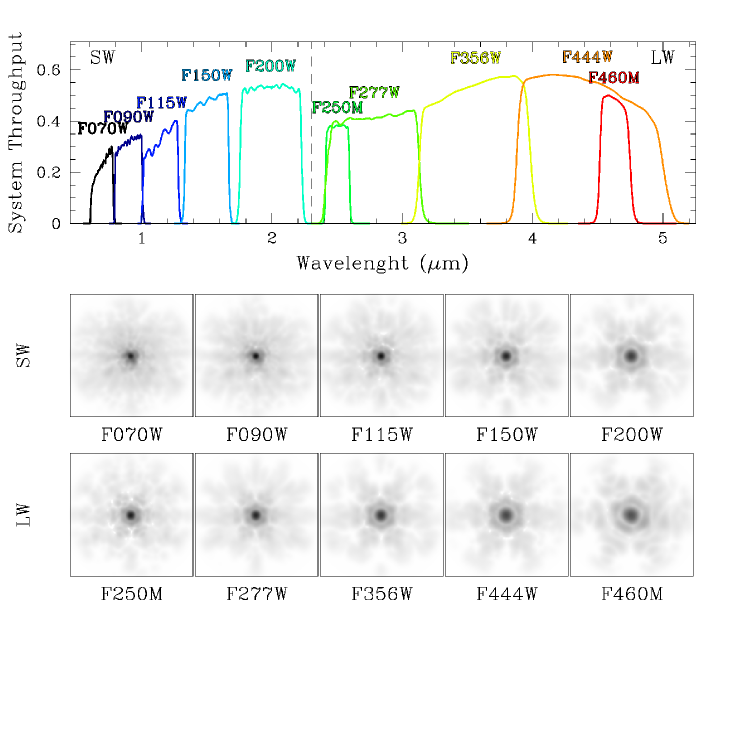
Figure 1: The JWST filters and ePSFs used in this work. Top panel shows the NIRCam + JWST total throughputs for the ten filters adopted in this work. The lower panels show the ePSFs in the central region of the detector A1 (SW channel, middle row) and ALONG (LW channel, bottom row) for all the filters used in this work.

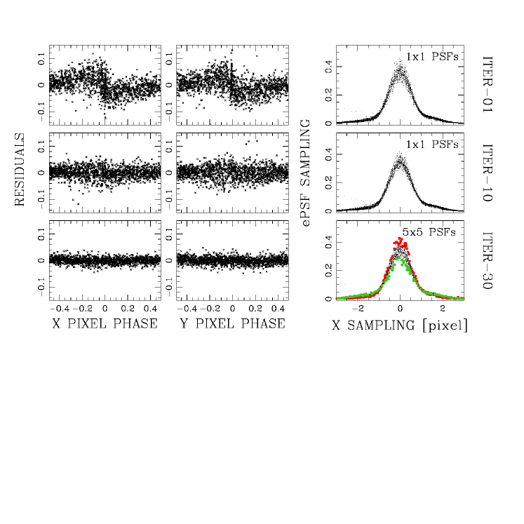
Figure 2: An overview of the improvements in the ePSF models during the different iterations. The top-to-bottom panels display the results for iteration 1, 10, and 30, respectively. The left and middle columns show the distributions of the pixel phase errors, representing the position residuals of the stars relative to their mean positions as a function of the X/Y pixel phase. The right panels show the ePSF sampling at various distances from the ePSF X centre within a slice of $-0.25<\delta Y<0.25$. In iteration 1 and 10, a single ePSF model was employed for the entire detector; in iteration 30, a grid of $5\times 5$ ePSFs was generated to account for the PSF variations across the detector. The green and red points represent the ePSF sampling for the lower-left and upper-right detector regions, respectively, demonstrating how the PSF peak changes across the detector. The figure showcases the case of the most undersampled filter, F070W, and focuses on modelling the ePSFs of detector A1.

2.1.1 Effective PSFs

For each filter and detector, we derived a $5\times 5$ grid of $4\times$ over-sampled library ePSFs by following the procedure developed by Anderson & King (2000, AK00) for undersampled PSFs, and employed in many other works (see, e.g, Anderson & King 2004, 2006; Anderson et al. 2015; Anderson 2016; Libralato et al. 2016a; Libralato et al. 2016b; Nardiello et al. 2016b; Libralato et al. 2023; Nardiello et al. 2023). Here, we provide a brief description of the ePSF modelling; we refer the reader to Paper I or AK00, for a detailed description of the method.

To obtain a well-sampled PSF model, we need to break the degeneracy between positions and fluxes of the sources which occurs when dealing with images whose PSFs are undersampled. The degeneracy can be broken by constraining the positions and fluxes of a set of stars using an iterative procedure. Initially, we extracted the first-guess positions and fluxes of bright, unsaturated, and isolated stars in each image using the ePSF grids obtained in Paper I. By employing the geometric distortion (GD) solution derived in Paper II, we determined the six-parameter transformations between the images by cross-matching the stars in common to different images. These transformations were employed to create a catalogue containing the mean positions and fluxes (transformed to a common reference system) of stars that were measured at least three times. This catalogue served as a master catalogue for ePSF modelling: indeed, stars in this catalogue will be adopted to break the degeneracy position-flux typical of undersampled images and derive the ePSF model.

The following four steps were followed to derive the ePSF model: (1) using the inverse GD solution from Paper II, we transformed the positions of the stars from the master catalogue to the reference system of each individual image; (2) we converted each pixel value within a radius of 25 pixels from each star’s centre into an estimate of the ePSF model, projecting the individual point samplings from the original image scale to a grid super-sampled by a factor 4 ($201\times 201$ points); (3) in iteration 1, we calculated the ePSF model as the 3$\sigma$-clipped average of the point sampling within a square by $0.25\times 0.25$ pixels² in ePSFs ($x,y$) coordinates. Starting from iteration 2, we first subtracted from each sampling the corresponding value of the last ePSF model, and then we calculated the 3$\sigma$-clipped average of the residuals in each $0.25\times 0.25$ pixels² grid point. Mean residuals are then added to the last available ePSF model and the result was smoothed with a combination of linear, quadratic and quartic kernels; (4) using the last available ePSF model, we re-measured the positions and fluxes of the sources in the master list in each image and we performed the transformations described above to obtain an updated master list to use in step (1).

We repeated steps (1)-(4) ten times assuming a single ePSF model for the entire detector; from iteration 11 we took into account the spatial variation of the ePSFs by dividing the image in sub-regions and calculating the ePSF models using the sources in each region. We gradually increased the number of subregions from $2\times 2$ (size of each subregion: $1024\times 1024$ pixel²) to $5\times 5$ (size of each subregion: $409\times 409$ pixel²).

Figure 2 illustrates the improvement of the ePSF models for the detector A1 and filter F070W (the most undersampled one) from the initial iteration to the final iteration (30). The enhancement is particularly evident in the distributions of the pixel phase errors, where the distributions flatten out as the PSF model improves (panels in the left and middle columns). Right column panels show the improvement of the ePSF samplings from iteration 1 to 10 when utilising a single PSF model for the entire detector, and in the final iteration where 25 different ePSFs are modelled. The ePSF samplings in the lower-left and upper-right regions, represented by green and red points respectively, demonstrate the significant variation of the PSF peak across the detector (see Appendix A).

Middle and bottom rows of Fig. 1 show the ePSFs in each filter, demonstrating how the ePSF model changes from a filter to another.

We make publicly available these ePSFs, which are improved with respect to our early derivation in Paper I, as at that time an appropriate geometric distortion correction was not publicly available. More details are reported in Appendix B.

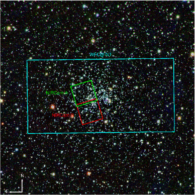
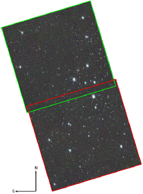
Figure 3: The left panel shows a three-colour image of a $30\times 30$ arcmin² region centred on NGC 2506, created by stacking $g-,r-,i-$sloan band images from the PS1 survey. The field of view of the observations obtained with NIRCam Module A and B is indicated by green and red squares, respectively. Additionally, the cyan rectangle represents the field of view of the WFC@INT detector 4 observations employed in this study (see Sect. 2.4). The right panel shows the three-colour image (F277W $+$ F356W $+$ F444W) generated by stacking the images obtained from the JWST observations employed in this work.

2.2 NGC 2506 JWST observations

Our target open cluster NGC 2506 was observed by JWST with NIRCam on November 1st, 2022 over the course of two hours, as part of the Calibration Program CAL-1538 (PI: Gordon). The purpose of this programme was to obtain observations of G dwarf stars for the absolute flux calibration of JWST. The observations consisted of a $2\times 2$ mosaic centred in ($\alpha,\delta$)=(120.03775,$-$10.78695), in which each dither is observed two times with RAPID readout mode (2 integrations comprising 2 groups of 1 frame, $t_{\rm exp}=42.947~{}s$). Data were collected in the same ten filters (8 wide $+$ 2 medium) employed in Sect. 2.1 and shown in Fig. 1.

Figure 3 illustrates the field of view covered by the NIRCam observations: in the left panel, a three-colour image obtained with PanSTARRS DR1 (PS1) images (Chambers et al. 2016; Magnier et al. 2020; Waters et al. 2020) is shown; green and red squares represent the Modules A and B field of views, respectively, which are also displayed in the right panel. Due to the limited overlap between the two modules and the scarcity of bright stars required for accurate six-parameter transformations, the data associated with the two modules were reduced separately. The final catalogues were combined at the end of the data reduction process.

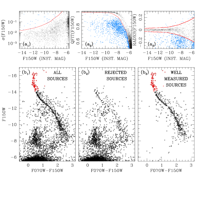
Figure 4: Overview of the procedure to identify and reject bad measurements in the catalogues produced by the KS2 routine. Panels (a₁), (a₂), and (a₃) show the distributions of photometric RMS ($\sigma$), quality-of-fit (QFIT), and RADXS for the filter F150W, respectively: red lines represent the threshold for good measurements in each parameter distribution, while the azure points are the rejected sources. Panels (b₁), (b₂), and (b₃) show the F150W versus (F070W$-$F150W) instrumental CMDs of all measured sources, the sources rejected in at least one filter, and the sources that passed the selection criteria in both filters, respectively. Saturated stars are plotted in red. The figure shows the sources in the catalogues obtained from Module A images.

2.2.1 Catalogues

Observations of NGC 2506 were obtained approximately four months after the data used to derive the library ePSFs. To account for the time variation of the PSFs, we employed the brightest and most isolated stars in each image to perturb the corresponding library PSFs (for a detailed description of the procedure, refer to Anderson & King 2006; Anderson et al. 2008; Nardiello et al. 2018b). To perturb the PSFs, we first measured the positions and fluxes of the stars selected for the perturbation with the library ePSF; we modelled and subtracted these stars from the image, and calculated the average of the residuals at different distances from the PSF centre (oversampled by a factor of 4). The mean residuals were utilised to adjust the PSF model. We iterated this procedure 5 times, using the last perturbed PSF each time.

We used the perturbed ePSFs to extract positions and fluxes of the stars in each image using the NIRCam version of the img2xym software, developed by Anderson et al. (2006) for the Wide Field Imager (WFI) @ESO/MPG 2.2m telescope. We will refer to this photometry as first-pass photometry. For each filter, we transformed positions and magnitudes to a common reference frame using six-parameter linear transformations and mean photometric zero points. Subsequently, we used the perturbed ePSFs, the images, and the transformations to perform the second-pass photometry with the KS2 software, developed by J. Anderson (which is a second generation of the software kitchen_sync presented in Anderson et al. 2008).

The KS2 software enables the measurement of positions and fluxes of bright and faint stars with high accuracy through the simultaneous analysis of all the images (see, e.g., Sabbi et al. 2016; Bellini et al. 2017; Nardiello et al. 2018b; Scalco et al. 2021), employing ad-hoc masks for bright and saturated stars (recovered during the first-pass photometry using the frame-0 of each image), and four different iterations in which progressively fainter stars are measured and subtracted from the images. During the first two iterations, we searched for sources in the F277W filter, in the third iteration we utilised the F356W filter, and in the fourth iteration we employed the F070W filter to identify faint blue sources that may not be detectable in the red filters.

Since only 45 % of the field of view of each module is covered by $\geq 3$ images per filter, while the remaining $\sim 55$ % is covered by two images (or even just one!) and since our goal is to identify as many weak sources as possible, the final catalogue generated by the KS2 software contains numerous sources that may be identified as noise peaks in individual images. Therefore, it is necessary to perform a "cleaning" of the catalogue. We adopted the same selection criteria as described in Nardiello et al. (2018b, 2019), which are based on the following parameters: (i) the photometric error (RMS); (ii) the quality-of-fit (QFIT), which assesses the PSF fitting of the source; (iii) the RADXS parameter defined as in Bedin et al. (2008), which enables the distinction between stellar sources, galactic-shaped sources, and cosmic-rays/noise peaks. A detailed description of these parameters is reported in Nardiello et al. (2018b), while an example of the selection process for the F150W filter is illustrated in panels (a) of Fig. 4. Additionally, sources measured only once and heavily contaminated by bright neighbouring stars were excluded from the selections. The lower panels of Fig. 4 display the instrumental F150W versus F070W$-$F150W colour-magnitude diagrams (CMDs) for all the detected sources (panel (b₁)), the sources rejected by the selections (panel (b₂)), and the sources that passed the selections (b₃)). Saturated stars (recovered from the first-pass photometry), that were not subjected to any selection, are highlighted in red.

2.2.2 Photometric calibration

We calibrated the catalogues in each filter and module in the VEGAmag system by using the most updated JWST photometric zero-points reported in the JWST User documentation. To calibrate the instrumental magnitudes, we first performed aperture photometry (with a radius $r_{\rm ap}=0.20$ arcsec) of the most isolated bright stars from each _cal image. We transformed the finite-aperture fluxes ${\rm FLX}(r_{\rm ap}=0.20^{\prime\prime}){\rm[MJy/sr]}$ into infinite-aperture fluxes using the Encircled Energy (EE) distributions reported in the JWST User documentation as follows:

$${\rm FLX}(r_{\rm ap}=\infty){\rm[MJy/sr]}={\rm FLX}(r_{\rm ap}=0.20^{\prime\prime}){\rm[MJy/sr]}/{\rm EE(0.20^{\prime\prime})}$$ (1)

We calculated the aperture photometry calibrated magnitudes by using the equation:

$$m_{\rm ap,cal}=-2.5\times\log{{\rm FLX[DN/s]}}+{\rm ZP}_{\rm VEGA}$$ (2)

where the flux ${\rm FLX[DN/s]}$ is computed as

$${\rm FLX[DN/s]}={\rm FLX}(r_{\rm ap}=\infty){\rm[MJy/sr]}/{\tt PHOTMJSR}$$ (3)

and ${\rm ZP}_{\rm VEGA}$ and ${\tt PHOTMJSR}$ are the photometric zero-points and the conversion factor MJy/sr to DN/s, respectively, tabulated in the JWST User documentation.

For each filter and module, we cross-matched the aperture photometry calibrated catalogues with the catalogue obtained in the previous section, and, for the $N_{\rm stars}$ stars in common, we calculated the difference

$$\delta m^{i}=m^{i}_{\rm ap,cal}-m^{i}_{\rm inst,KS2}\,\,\,\,\,\,{\rm with\,}i=1,...,N_{\rm stars}$$ (4)

where $m_{\rm inst,KS2}$ is the magnitude output of the KS2 routine. We then computed the average value of $\delta m$, which represents the photometric zero-point to be added to the instrumental magnitudes.

Due to the errors in the photometric zero-points, which are $\sim 0.02$ mag, we observed slight discrepancies between the CMDs obtained from the stars measured in Module A and Module B images. To align the two modules to a common reference system, we employed the following approach: we used a small sample of stars that were detected in both modules (consisting of 10 to 25 stars) to determine the mean difference between the magnitudes obtained from the images of Module A and Module B ($\delta m$(A-B)). Subsequently, we applied a correction by subtracting (or adding) $\delta m$(A-B)/2 to the magnitudes of the stars in Module A (or Module B). An example of the achieved results can be seen in panel (a) of Fig. 5.

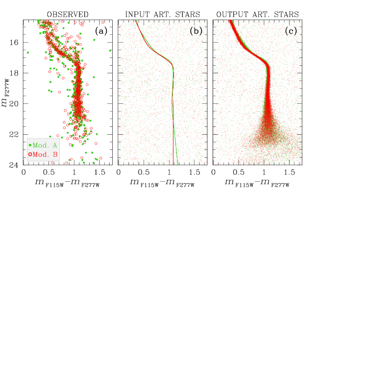
Figure 5: Observed and artificial $m_{\rm F277W}$ versus $m_{\rm F115W}-m_{\rm F277W}$ CMDs for Module A (in green) and B (in red). Panel (a) shows the CMD obtained with real observations; panel (b) and (c) display the input and output artificial star CMDs.

2.2.3 Artificial stars

We employed artificial stars to assess the completeness of our catalogue across different filters (Sect.3.2 and Nardiello et al. 2018a for detailed information). For each module, we generated 50 000 artificial stars (ASTs) within the F277W magnitude range from $14.5$ (near the saturation limit) to $26.5$. We created 40 000 ASTs with a flat luminosity function in F277W and with colours that lie along the cluster sequence in the different $m_{\rm F277W}$ versus $m_{\rm X}-m_{\rm F277W}$ CMDs, where X is one of the ten available filters. Additionally, we generated other 10 000 ASTs with a flat luminosity function in F277W and with random colours in the different filters, to simulate the field stars. The spatial distribution of the ASTs was uniform across the field of view. The CMD of the input catalogue of ASTs is shown in panel (b) of Fig. 5. We used the KS2 software to add one AST at a time to each image with the appropriate position and flux, adopting the same procedure used for real stars to search and measure the added AST. The software provided output parameters for the ASTs identical to those of real stars. Panel (c) of Fig. 5 showcases the CMD of the ASTs output of KS2 routine.

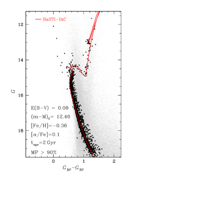
Figure 6: The $G$ versus $G_{\rm BP}-G_{\rm RP}$ CMD obtained with the Gaia DR3 catalogue of the stars within 1.5 deg. from the cluster centre. Black and grey stars are the sources identified as bona-fide cluster members and Galactic stars, respectively, based on the MP (threshold 90 %); for comparison, a BaSTI-IAC 2 Gyr isochrone is plotted in red by adopting the parameters reported in the panel.

Table 1: Cluster parameters of NGC 2506.

Parameter	Value	Reference
$\alpha$(ICRS, J2015.5) [deg.]	120.010	(1)
$\delta$(ICRS, J2015.5) [deg.]	$-$10.773	(1)
$l$(J2015.5) [deg.]	230.56942	(1)
$b$(J2015.5) [deg.]	+09.93816	(1)
$d$ [pc]	$3100\pm 175$	this work
$(m-M)_{0}$	$12.46\pm 0.12$	this work
$E(B-V)$	$0.08\pm 0.01$	this work
[Fe/H] [dex]	$-0.36\pm 0.10$	(2)
[$\alpha$/Fe] [dex]	$0.10\pm 0.10$	(2)
[M/H] [dex]	$-0.29\pm 0.10$	(2)
tage [Gyr]	$2.01\pm 0.10$	(2)
$r_{\rm c}$ [arcmin]	$2.60\pm 0.05$	this work
$r_{\rm c}$ [pc]	$2.34\pm 0.05$	this work
$r_{\rm t}$ [arcmin]	$33.0\pm 4.3$	this work
$r_{\rm t}$ [pc]	$29.8\pm 3.9$	this work
Notes: (1) Tarricq et al. (2021); (2) Knudstrup et al. (2020)

2.3 NGC 2506 from the Gaia archive

We adopted the Gaia DR3 catalogue (Gaia Collaboration et al. 2021, 2022) to obtain information about stars located within a radius of 1.5 degrees from the cluster centre ($\alpha_{c},\delta_{c}$)=($120.010,-10.773$) (Tarricq et al. 2021). We calculated the membership probabilities (MPs) using the method outlined in Griggio & Bedin (2022), which considers the spatial distribution, proper motion, and parallax of the sources. The bona-fide cluster members, with a membership probability $>90~{}\%$, are denoted in black in Fig. 6. We performed a cross-match between the bona-fide cluster members and the catalogue by Bailer-Jones et al. (2021) and determined the mean distance of the cluster to be $d=3100\pm 175$ pc, consistent with the value reported by Knudstrup et al. (2020). Using the Infrared Dust Maps (Schlegel et al. 1998; Schlafly & Finkbeiner 2011), we found a mean reddening $E(B-V)=0.08$ for the cluster. Knudstrup et al. (2020) determined the age, metallicity, and $\alpha$-enhancement of NGC 2506 through the analysis of detached eclipsing binaries, yielding $t_{\rm age}\sim 2$ Gyr, [Fe/H] $\sim-0.36$, and [$\alpha$/Fe] $\sim 0.10$, respectively. Adopting these cluster parameters (reported in Table 1), we plotted a 2 Gyr BaSTI-IAC isochrone (Hidalgo et al. 2018, in red; Pietrinferni et al. 2021, in red) in the $G$ versus $G_{\rm BP}-G_{\rm RP}$ CMD. This $\alpha$-enhanced IAC-BaSTI isochrone has been derived as follows. We have first downloaded from the BaSTI-IAC website solar-scaled and $\alpha$-enhanced ([$\alpha$/Fe]=0.4) isochrones (including overshooting and atomic diffusion) for [Fe/H]=$-$0.36, and then interpolated linearly in [$\alpha$/Fe] (between 0 and 0.4) to obtain isochrones with [Fe/H]=$-$0.36 and [$\alpha$/Fe]=0.1 (see Table 1) – corresponding to a total metallicity [M/H]=$-$0.29.

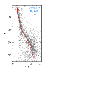
Figure 7: The $I$ versus $V-I$ CMD obtained with the WFC@INT data. A BaSTI-IAC 2 Gyr isochrone is plotted in red.

2.4 Ground-based observations of NGC 2506

We have also taken advantage of data obtained with the Wide Field Camera (WFC) mounted at the prime focus of the 2.5m Isaac Newton Telescope (INT) for Programme I9/2003B (PI: Rosenberg). The observations were conducted between January 21 and 22, 2004. The dataset includes the following exposures: $3\times 300$ s $+$ $2\times 600$ s $V$-Harris images and $1\times 30$ s $+$ $2\times 900$ s $i$-Sloan images. All observations were taken at an airmass between 1.32 and 1.48 and the typical seeing was around 1-1.2 arcsec. For this work, only images associated with CCD#4, which contains the JWST observations, were used (as shown in Fig. 3).

We reduced the dataset by using empirical PSFs and the software developed by Anderson et al. (2006) adapted for WFC@INT images. We corrected the geometric distortion by following the procedure adopted by Griggio et al. (2022). We calibrated the $V,i$ magnitudes into $V$-Johnson and $I$-Cousins respectively, by using the homogeneous photometry published by P. .B. Stetson (Stetson 2000).

The resulting $I$ versus $V-I$ CMD from WFC@INT data is shown in Fig. 7, together with a 2 Gyr BaSTI-IAC isochrone adopting the same chemical composition, reddening, and distance as in the comparison with the Gaia data. The isochrone matches the pattern of the CMD distribution of the observed stars reasonably well for $I\lesssim 19.5$.

3 Astrometric and photometric analyses

3.1 Proper motions and membership probabilities

To extend the membership study to magnitudes beyond the reach of Gaia (i.e., for stars fainter than $G\simeq 19$), we used proper motions derived from JWST and INT positions. We discriminated between cluster members and field stars, following the methodology employed in previous studies by our research group (see, e.g., Bedin et al. 2003; Anderson et al. 2006; Bellini et al. 2010; Libralato et al. 2014; Nardiello et al. 2015; Nardiello et al. 2016a). To achieve this, we calculated the displacements of stars between two different epochs after transforming their positions to a common reference system using 6-parameter global transformations. The first epoch was represented by the WFC@INT data, with a mean epoch of $t_{\rm I}=2004.06$, while for the second epoch we took advantage of the NIRCam catalogues, with $t_{\rm II}=2022.84$. We determined the relative displacements of the stars, referring them to the average motion of the cluster, over a time span $\Delta t_{\rm II-I}=18.78$ years.

We computed the membership probability (MP) for each of these faint stars in the catalogues, following an approach similar to that described by Griggio & Bedin (2022). Only proper motions were considered in the calculation of the MPs, without incorporating spatial and parallax terms. Specifically, the spatial term was neglected due to the limited field of view of JWST observations, which allowed us to assume a uniform distribution of the cluster’s stars within the observed area, while parallaxes are not available for these faint stars.

Figure 8 illustrates the selection of cluster members based on MPs. In the range $16.0<m_{\rm F070W}\leq 20.5$, stars with MP$>90~{}\%$ were chosen as cluster members. For saturated stars and faint stars with $m_{\rm F070W}>20.5$, we relaxed the selection criteria and identified cluster members with MP$>50~{}\%$ and MP$>75~{}\%$, respectively, as indicated in panel (d) (magenta line). Relative proper motions are shown in panels (a) (as a function of the colour $m_{\rm F070W}-m_{\rm F444W}$) and (b), while panel (c) shows the $m_{\rm F070W}$ versus $m_{\rm F070W}-m_{\rm F444W}$ CMD for cluster members (black) and field objects, mainly Galactic field stars (azure).

3.2 Completeness

By using the ASTs obtained as described in Section 2.2.3, we determined the completeness in different regions of the field of view and for different magnitudes. The completeness is calculated as the ratio between the number of recovered stars and the number of injected stars, $N_{\rm rec}/N_{\rm inj}$. We considered an AST as recovered if the differences in position satisfy $|x_{\rm in}-x_{\rm out}|<1$ px and $|y_{\rm in}-y_{\rm out}|<1$ px; additionally, we applied the following magnitude conditions: $|m_{\rm F277W,in}-m_{\rm F277W,out}|<0.5$ for stars measured in iteration 1 or 2, $|m_{\rm F356W,in}-m_{\rm F356W,out}|<0.5$ for ASTs measured in iteration 3, and $|m_{\rm F070W,in}-m_{\rm F070W,out}|<0.5$ for sources measured in iteration 4. These conditions reflect the procedure used to identify real stars. To account for the rejections described in Sect. 2.2.1, we applied to the ASTs the same selections used for real stars, and included them in the computation of $N_{\rm rec}$.

Figure 9 shows the completeness as a function of the magnitude and position. The left panels demonstrate how completeness varies with magnitude for different image coverages: when stars are observed just once or two times, completeness is lower than 60 %, and drops below 50 % at $m_{\rm F277W}\sim 21$ (dark grey points). For stars measured in at least 3 images the completeness is 20-30 % higher, and it is lower than 50 % at $m_{\rm F277W}\sim 22.5$ (magenta and orange points). The right panel shows the dependence of completeness on position due to varying image coverage: the blue/azure squares of each module are the regions covered by $\geq 4$ images, and 50 % completeness is reached at magnitude $m_{\rm F277W}\sim 21.5$–$22.5$; green/red regions are areas covered by $\leq 2$ images, where completeness reaches 50 % at $m_{\rm F277W}\sim 20.0$–$21.0$.

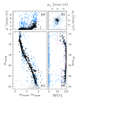
Figure 8: Cluster membership analysis using the WFC@INT and NIRCam@JWST data. Panel (a) shows the distribution of proper motions relative to the cluster’s mean motion, as a function of the $m_{\rm F070W}-m_{\rm F444W}$ colour; panel (b) presents the relative proper motions of the stars common to both datasets. Panel (c) is the $m_{\rm F070W}$ versus $m_{\rm F070W}-m_{\rm F444W}$ CMD of the stars in the fields of the two modules: grey squares are the stars not measured in the WFC@INT data set. Panel (d) showcases the MP distribution; the magenta line denotes the MP threshold used in this work. In all panels, cluster members are represented by black points, while field stars are denoted by azure points.

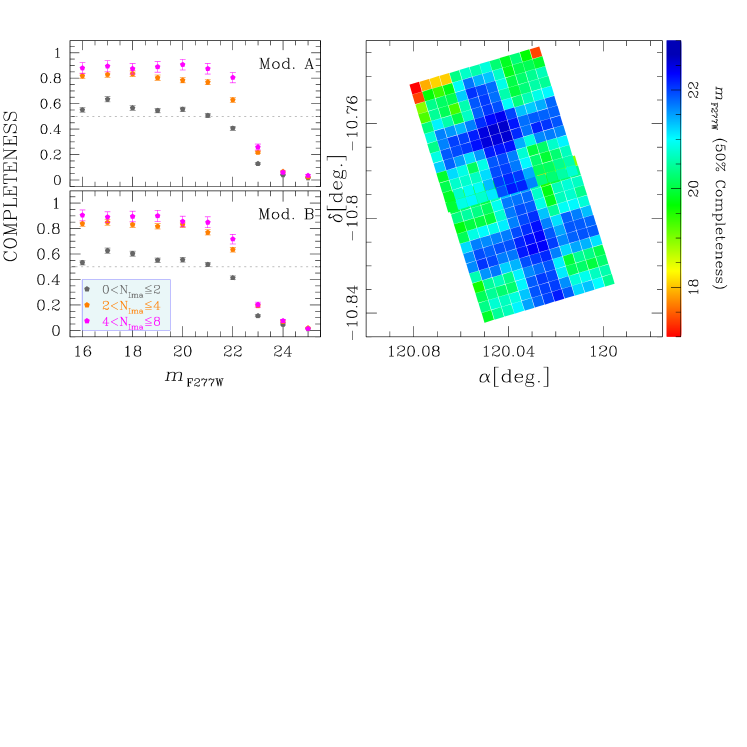
Figure 9: Analysis of the completeness of our catalogues: the left panels show the completeness as a function of the $m_{\rm F277W}$ magnitude for Module A (upper panel) and B (bottom panel). Magenta, orange, and dark grey points represent the completeness distribution in the case the stars appear in less than 3, between 2 and 4, and between 4 and 8 images, respectively. The right panel shows the completeness as a function of the position: we calculated the $m_{\rm F277W}$ limit magnitude for which the completeness reaches 50 % in squares of 15.5$\times$15.5 arcsec², coloured following the colour-bar on the right.

3.3 Colour-magnitude diagrams

Figure 10 shows a rundown of the CMDs with the ten available filters: grey and black points are the stars that passed the quality and membership selections, respectively. Naturally, these CMDs have different levels of completeness along the MS. As already done in Sect. 2.3 and 2.4, we superimposed 2 Gyr BaSTI-IAC isochrones (in red) to the JWST CMDs. The lower mass limit of the isochrones is 0.1 $M_{\odot}$. Some filters combinations, as for example $m_{\rm F150W}$ vs $(m_{\rm F115W}-m_{\rm F150W})$ or $m_{\rm F150W}$ vs $(m_{\rm F150W}-m_{\rm F356W})$, allow us to reach a magnitude limit $m_{\rm F150W}\sim 22$ with SNR$\sim 10$; according to the models, this magnitude limit corresponds to masses below $0.1M_{\odot}$ on the main sequence.

We investigated the lower MS of NGC 2506 to check the presence of broadening due to chemical variations. The analysis is shown in Fig. 11: we compared the $m_{\rm F150W}$ vs $(m_{\rm F115W}-m_{\rm F150W})$ CMD of NGC 2506 against the HST $m_{\rm F160W}$ vs $(m_{\rm F110W}-m_{\rm F160W})$ CMD of the old, metal-poor, massive globular cluster NGC 6752 (leftmost panel, Scalco et al. in prep.). As reported by Milone et al. (2019), the multiple lower MSs in NGC 6752 are due to the variations of Oxygen between the stars belonging to different stellar populations. We shifted the CMD of NGC 6752 in colour and magnitude in such a way that the "knee" of the MS overlaps the one of the NGC 2506’s CMD: the middle panel of Fig. 11 demonstrates that the lower MS of NGC 2506 agrees with a single sequence of NGC 6752 and that no chemical variation is expected among the low-mass stars of this cluster. As a further test, we simulated the CMD of a single population by selecting randomly 600 ASTs (about the number of observed stars in the MS) from the sample of ASTs; we also simulated 57.5 % MS-MS binaries (with a flat mass-ratio distribution, see Sect. 5). The simulated CMD is reported in right-hand panel of Fig. 11: it demonstrates that the observed CMD agrees with the simulated CMD of a single stellar population.

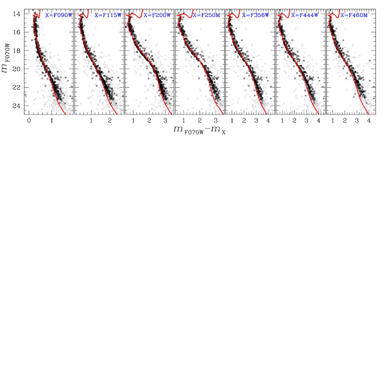
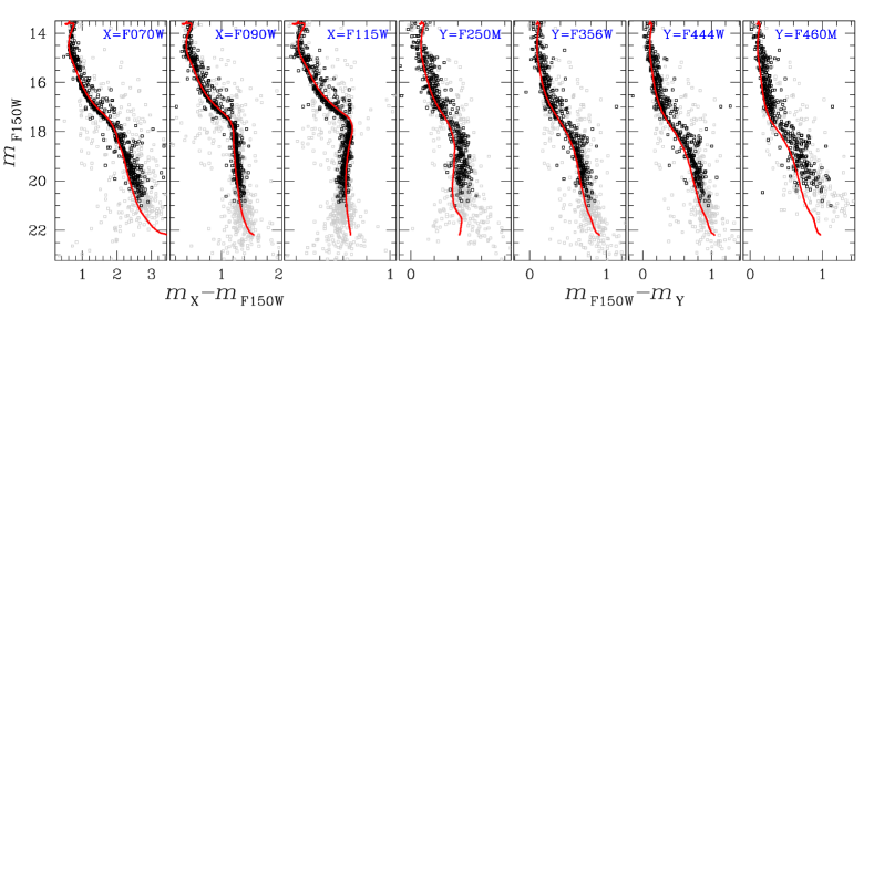
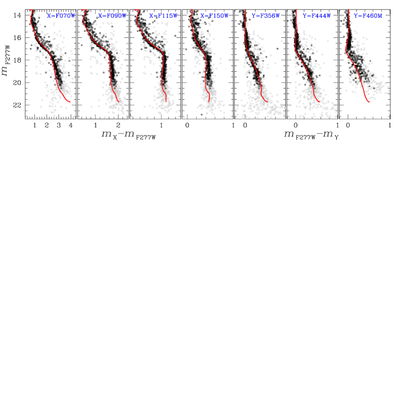
Figure 10: Some of the possible CMDs obtained with the available JWST photometry in different filters: panels in top row show the $m_{\rm F070W}$ vs $(m_{\rm F070W}-m_{\rm X})$ CMDs with X=F090W, F115W, F200W, F250M, F356W, F444W, F460M; panels in the middle row are the $m_{\rm F150W}$ vs $(m_{\rm X}-m_{\rm F150W})$ CMDs with X=F070W, F090W, F115W, and the $m_{\rm F150W}$ vs $(m_{\rm F150W}-m_{\rm Y})$ CMDs with Y=F250M, F356W, F444W, F460M; in the bottom row are shown the the $m_{\rm F277W}$ vs $(m_{\rm X}-m_{\rm F277W})$ CMDs with X=F070W, F090W, F115W, F150W and the $m_{\rm F277W}$ vs $(m_{\rm F277W}-m_{\rm Y})$ CMDs with Y=F356W, F444W, F460M. 2 Gyr BaSTI-IAC isochrones are plotted in red.

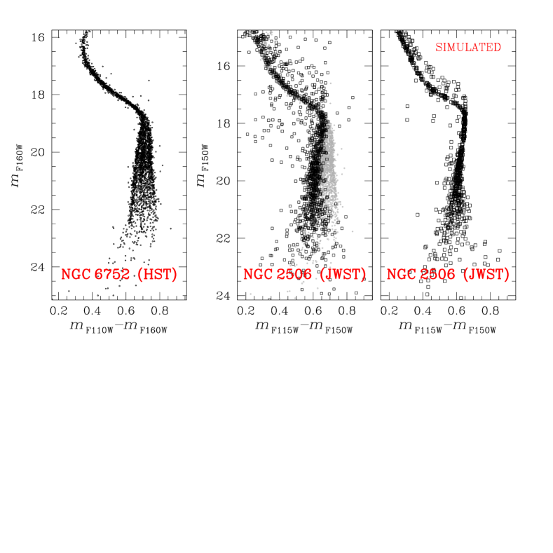
Figure 11: Comparison between lower MS of NGC 6752 (three stellar populations) and NGC 2506 (single population) is similar IR filters. Left panel shows the HST $m_{\rm F160W})$ vs $(m_{\rm F110W}-m_{\rm F160W})$ CMD of NGC 6752, for which three different low-MSs are well detectable. Middle panel is a comparison between the CMD of NGC 6752 (grey points) and the $m_{\rm F150W})$ vs $(m_{\rm F115W}-m_{\rm F150W})$ CMD of NGC 2506 (black points), that demonstrates that the lower-MS of the open cluster agrees with the presence of a single population. This is also demonstrated by the simulated CMD shown in the right panel.

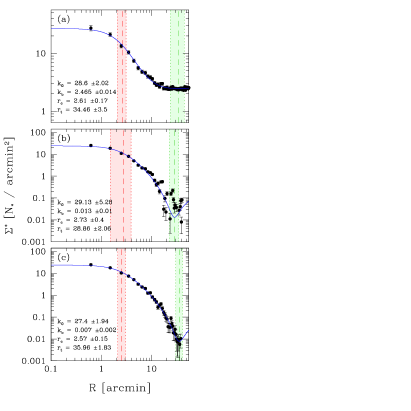
Figure 12: Radial stellar density profiles of NGC 2506, calculated for stars with magnitudes between $G=14$ and $G=18$ in the Gaia DR3 catalogue. The profiles are obtained by dividing the cluster region into annuli of 1 arcmin width. The three panels display different approaches: panel (a) shows the density profile modelling both cluster and Galactic field stars; in panel (b), the mean density of background stars is subtracted from the density profile of panel (a); panel (c) showcases the density profile with each star’s contribution weighted by MP. The observed density profile is represented by black points, and a King profile function is fitted to the three profiles (blue lines). The vertical dashed lines in red and green denote the core and tidal radii, respectively, with shaded regions representing the corresponding $\pm 1\sigma$ errors. The parameters of the King profile function are listed within each panel.

4 Radial density profile

We computed the radial stellar density profile of NGC 2506 by using the Gaia DR3 catalogue. The results are presented in Fig. 12. To obtain the density profile, we divided the area within a radius of 70 arcmin into a series of annuli with a 1 arcmin width. For each annulus, we computed the number of stars per arcmin² ($\Sigma^{\star}$) and the mean radial distance of the stars from the centre ($R$). We restricted our analysis to stars with magnitudes between $G=14$ and $G=18$, which –in the average Galactic field– should have a completeness close to 100 % (Boubert & Everall 2020; Everall & Boubert 2022).

To fit the density profile distributions shown in Fig. 12, we employed a King profile (King 1962), described by the function:

$$\Sigma^{\star}[R]=k_{\rm b}+k_{\rm 0}\left(\frac{1}{\sqrt{1+R^{2}/r_{\rm c}^{2}}}-\frac{1}{\sqrt{1+r_{\rm t}^{2}/r_{\rm c}^{2}}}\right)^{2}$$ (5)

where $k_{\rm b}$ and $k_{\rm 0}$ represent the background and central stellar densities, respectively, $r_{\rm c}$ is the core radius, and $r_{\rm t}$ denotes to the cluster tidal radius.

We analysed the density profile of NGC 2506 in three different cases, shown in the three panels in Fig. 12. In case (a), we fitted a density profile that model the contribution of both the cluster stars and the Galactic field stars. In case (b), we subtracted the mean density of background stars from the calculated stellar density in each annulus. The background density was determined in an annulus ranging from $R=70$ to $R=90$ arcmin from the cluster centre. In case (c), we fitted a density profile in which the contribution of each star is weighted by the MP. Excluding the background density $k_{\rm b}$, which is higher in case (a) due to the inclusion of Galactic field stars in the fit, the other parameters, such as $k_{0}$, $r_{\rm c}$, and $r_{\rm t}$, show consistent values, and they agree within 3$\sigma$. The weighted mean values we obtained are as follows: $k_{0}=28.1\pm 0.9$ stars/arcmin², $r_{\rm c}=2.60\pm 0.05$ arcmin, and $r_{\rm t}=33.0\pm 4.3$ arcmin.

The core radius we measured is smaller than the value reported by Rangwal et al. (2019) based on WFI and Gaia DR2 data, although they agree within 3.2$\sigma$. However, our core radius agrees with the value found by Lee et al. (2013) for stars with $V<17$ magnitude. The central density and tidal radius obtained in our study are higher than those reported by Rangwal et al. (2019, 16.58 stars/arcmin² and 12 arcmin, respectively), with a difference $>10\sigma$. This discrepancy may be attributed to differences in the selection of the cluster members and/or the different density profile models used in the analysis. Additionally, Lee et al. (2013) found a smaller tidal radius ($\sim 19$ arcmin). These discrepancies can also be explained by the presence of tidal tails extending out to 1 degree from the cluster centre, as reported by Gao (2020, even if we did not detect any well defined tail as in this work).

5 Binaries and mass functions

By combining Gaia DR3 and JWST data, we performed an analysis to determine the fraction of photometric binaries, as well as the luminosity and mass functions for MS stars. This analysis considered stars located at different distances from the cluster centre and within various mass intervals.

5.1 Main sequence Photometric binaries

At the distance of NGC 2506 essentially all binaries are unresolved. An unresolved binary system composed of two MS stars with magnitudes $m_{1}$ and $m_{2}$, corresponding to fluxes $F_{1}$ and $F_{2}$, can be treated as a point-like source with a total magnitude given by:

$$m_{\rm bin}=m_{1}-2.5\log{\left(1+\frac{F_{2}}{F_{1}}\right)}$$ (6)

The ratio $F_{2}/F_{1}$ is strongly correlated with the mass ratio $q=M_{2}/M_{1}$, where $M_{1}$ represents the mass of the primary (more massive) star and $M_{2}\leq M_{1}$. In the case of $M_{2}=M_{1}$, the magnitude of the binary system is $\sim 0.75$ magnitudes brighter than that of the primary component. Thus, the $q=1$ case serves as a limit for the redder and brighter section of the MS, where MS-MS binaries are located.

To estimate the fraction of binaries, we employed the JWST and Gaia DR3 catalogues following the approach described by Milone et al. (2012, 2016) and Cordoni et al. (2023), and shown in Fig. 13. Briefly, we defined a region R_I encompassing MS stars and binaries with $q<q^{\rm lim}$, where $q^{\rm lim}$ denotes the mass ratio below which is difficult to discriminate between single and binary stars in the CMD. In this study, we used $q^{\rm lim}=0.6$, represented as an orange line in Fig. 13, which was determined by fitting the BaSTI-IAC isochrones discussed in the previous sections. To define the bluer limit of R_I, we calculated the standard deviation of the colour ($\sigma_{\rm col}$) at various magnitudes along the MS. We considered all the stars whose colour is $>{\rm col}_{\rm fid}-2.5\sigma_{\rm col}$, where ${\rm col}_{\rm fid}$ represents the colour of the MS fiducial line. In the case of Gaia CMD, we used the $G_{\rm BP}-G_{\rm RP}$ colour, while for the JWST data we adopted the $m_{\rm F070W}-m_{\rm F277W}$ wide colour baseline. The region R_I is confined within the magnitude intervals $16.15\leq G_{\rm RP}\leq 18.15$ in the case of Gaia CMD, and $15.50\leq m_{\rm F277W}\leq 18.50$ for the JWST data. All the stars in the region R_I are plotted in red in Fig. 13. The region R_II is defined as the area between the lines determined by binary systems with $q=0.6$ (represented by the orange line) and $q=1$ shifted by $2.5\sigma_{\rm col}$. The faint and bright limits of R_II correspond to the positions of binary systems with mass ratios $0\leq q\leq 1$. In Fig. 13, stars located within the region R_II are shown in green.

In the case of Gaia DR3, we assumed a completeness of the catalogue equal to 100 %, and we calculated the fraction of binaries with mass ratios $q\geq 0.6$ using the following formula:

$$f_{\rm bin}^{q\geq 0.6}=\frac{\sum_{i}{w^{i}_{\rm MP}}}{\sum_{j}{w^{j}_{\rm MP}}}\,\,\,\,\,{\rm with\,\,\,}i=1,...,N_{\rm II};\,\,\,j=1,...,N_{\rm I}$$ (7)

where $w_{\rm MP}$ is a weight ranging from 0 to 1 corresponding to membership probabilities from 0 % to 100 %, and $N_{\rm I}$ and $N_{\rm II}$ represent the number of sources within the region R_I and R_II, respectively.

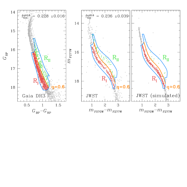
Figure 13: Procedure employed to determine the MS binary fraction from the Gaia DR3 $G_{\rm RP}$ vs $(G_{\rm BP}-G_{\rm RP})$ CMD (left panel), and the JWST $m_{\rm F277W}$ vs. $(m_{\rm F070W}-m_{\rm F277W})$ CMD (middle and right panels). Each CMD is divided in two regions: (i) R_I contains the majority of MS and low mass-ratio binary stars (red points); (ii) R_II includes the binaries with mass ratios between $q=0.6$ and $q=1.0$, while also accounting for the uncertainties in colours and magnitudes (green points). The right panel shows the simulated JWST CMD, which was used to assess the impact of photometric errors and blending on the computation of the binary fraction. The primary mass interval covered in the Gaia DR3 data analysis is $0.75\lesssim M\lesssim 1.10~{}M_{\odot}$, while in the case of JWST data we studied binaries in the primary mass interval $0.45\lesssim M\lesssim 1.05~{}M_{\odot}$.

In the case of JWST data, we took into account the completeness of our catalogue as well as the effects of photometric errors and blending, which can increase the number of sources in region R_II. To address this issue, we made use of ASTs to simulate a CMD as follows: for each real star in our catalogue that passed the quality selections and had membership probabilities $>90~{}\%$, we randomly selected a star from the ASTs catalogue located within a radius $r_{\rm AST}=3$ arcsec from the target star, with a maximum difference in F277W magnitude of $\delta m_{\rm F277W,AST}=1$ mag. The simulated CMD is shown in the right panel of Fig. 13. For the JWST data, we estimated the fraction of MS binaries with mass ratios $q\geq 0.6$ using the following equation:

$$f_{\rm bin}^{q\geq 0.6}=\frac{\sum_{i}{w^{i}_{\rm MP}/c^{i}}}{\sum_{j}{w^{j}_{\rm MP}/c^{j}}}-\frac{N^{\rm AST}_{\rm II}}{N^{\rm AST}_{\rm I}}\,\,\,\,\,{\rm with\,\,\,}i=1,...,N_{\rm II};\,\,\,j=1,...,N_{\rm I}$$ (8)

where $w_{\rm MP}$ is the weight defined earlier, $c$ denotes the completeness associated with each star, and $N^{\rm AST}_{\rm I}$ and $N^{\rm AST}_{\rm II}$ correspond to the number of simulated stars that fall within R_I and R_II, respectively. For the region covered by the Gaia DR3 catalogue ($0\lesssim R\lesssim 35$ arcmin), we obtained $f_{\rm bin}^{q\geq 0.6}=0.228\pm 0.016$ in the primary mass interval $0.75\lesssim M\lesssim 1.10~{}M_{\odot}$, while for the region covered by JWST data ($0.2\lesssim R\lesssim 4.6$ arcmin) we measured $f_{\rm bin}^{q\geq 0.6}=0.236\pm 0.039$ in the primary mass range $0.45\lesssim M\lesssim 1.05~{}M_{\odot}$. Supposing a flat mass-ratio distribution (Milone et al. 2012), the total fraction of MS-MS binary stars with q$>0$ is $\sim 0.575$.

We investigated the binary fraction as a function of the mass of the primary star. To measure the binary fraction in different mass intervals, we followed the procedure described earlier while adjusting the lower and upper magnitude limits of the R_I region. The results are shown in the top panel of Fig.14 and in Table 2: the binary fraction measured in the entire field using Gaia DR3 data is reported in black for four different mass intervals, the binary fraction measured with Gaia in the overlapping region with JWST is shown in magenta, and the binary fraction calculated using JWST data down to 0.45 $M_{\odot}$ is represented in blue. We performed a $\chi^{2}$ test to assess the flatness of the $f_{\rm bin}^{q\geq 0.6}$ distribution as a function of the mass of the primary star. Considering all the data points and their corresponding errors from the top panel of Fig. 14, we constructed a histogram with three bins and calculated the $\chi^{2}$ between the observed and expected frequencies, resulting in $\chi^{2}=0.67$. Subsequently, using the $\chi^{2}$-distribution, we determined the P-value, which represents the probability that the distribution is flat. The obtained P-value was $\sim 72~{}\%$.

Furthermore, we computed the radial distribution of the binary fraction for both the Gaia and JWST datasets, as illustrated in the bottom panel of Fig. 14 and in Table 2. For this distribution, we divided the Gaia and JWST samples into radial bins, each containing an equal number of stars. The three measurements obtained with Gaia are denoted by black squares, while the two measurements from JWST are represented by blue circles. These measurements exhibit a radial trend, with a higher concentration of binaries in the central region. We also examined the consistency between the Gaia and JWST measurements in the overlapping region of the two datasets, displayed by the magenta triangle and orange circle. The P-value test yielded a probability of $\sim 41~{}\%$ that the distribution is flat, suggesting a plausible radial trend in the binary fraction.

Table 2: Analysis of photometric binaries in NGC 2506.

$f^{q\geq 0.6}_{\rm bin}$ vs $M^{\rm prim}$
Region	$M^{\rm prim}$ interval	Mean $M^{\rm prim}$	$f^{q\geq 0.6}_{\rm bin}$
	($M_{\odot}$)	($M_{\odot}$)
Gaia (All)	0.76–0.83	0.79	$0.203\pm 0.030$
	0.83–0.92	0.87	$0.155\pm 0.025$
	0.92–1.01	0.96	$0.213\pm 0.032$
	1.01–1.10	1.05	$0.240\pm 0.037$
Gaia (JWST region)	0.78–0.94	0.86	$0.249\pm 0.065$
	0.94–1.13	1.04	$0.287\pm 0.079$
JWST	0.44–0.59	0.51	$0.143\pm 0.059$
	0.59–0.81	0.68	$0.240\pm 0.070$
	0.81–1.06	0.94	$0.248\pm 0.059$
$f^{q\geq 0.6}_{\rm bin}$ vs $R$
Region	$R$ interval	Mean $R$	$f^{q\geq 0.6}_{\rm bin}$
	(arcmin)	(arcmin)
Gaia (All)	0.08–4.00	2.38	$0.273\pm 0.035$
	4.00–8.58	5.98	$0.185\pm 0.025$
	8.58–40.48	12.97	$0.233\pm 0.028$
Gaia (JWST region)	0.24–4.61	2.37	$0.289\pm 0.053$
JWST (1 bin)	0.24–4.61	2.51	$0.237\pm 0.040$
JWST (2 bin)	0.24–2.26	1.64	$0.313\pm 0.075$
	2.26–4.61	3.03	$0.191\pm 0.045$

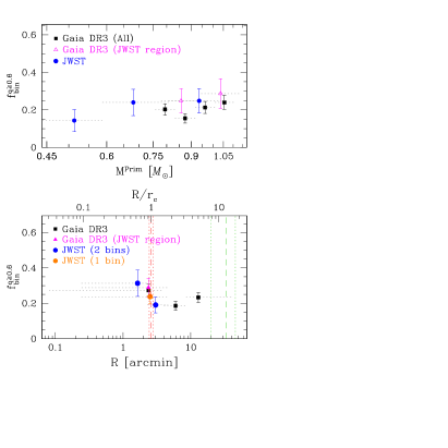
Figure 14: Analysis of the binary fraction as a function of the mass of the primary star (top panel) and of the radial distance from the cluster centre (bottom panel). Black squares, magenta triangles, and blue circles refer to the analysis performed with the entire Gaia DR3 catalogue, the Gaia DR3 catalogue limited to the JWST region, and the JWST data, respectively. The orange point in the bottom panel is referred to the analysis performed with JWST in only one radial interval.

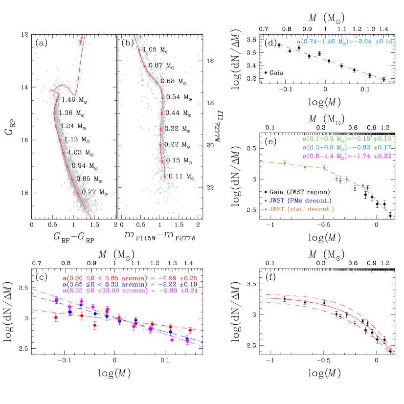
Figure 15: An overview of the procedure to calculate the MS MFs from Gaia DR3 and JWST data. Panels (a) and (b) show the $G_{\rm RP}$ vs $(G_{\rm BP}-G_{\rm RP})$ and $m_{\rm F277W}$ vs $(m_{\rm F115W}-m_{\rm F277W})$ CMDs, respectively, with superimposed in red the BaSTI-IAC isochrones marking the mass intervals on the MS. Panels (c) and (d) show the MFs calculated in three radial intervals and over the whole field, respectively, using the Gaia DR3 dataset; slopes ($\alpha$) of the fitted straight lines are reported inside the panels. Panels (e) and (f) show the MF obtained using the stars in the JWST region and combining Gaia and JWST data. For JWST data we adopted two different approaches based on the PMs and statistical decontamination. In panel (e) the MF is fitted with three different straight lines ($\alpha$ slopes are reported in the panel) corresponding to different mass intervals. In panel (f) we adopted a logistic function (see text for details).

Table 3: MFs of MS stars in NGC 2506.

Global MF from Gaia DR3 catalogue
R interval	$M$ interval	Mean $M$	$({\rm dN}/\Delta M)$
(arcmin)	($M_{\odot}$)	($M_{\odot}$)
0.00–33.00	0.74–0.79	0.77	$5168\pm 335$
	0.79–0.84	0.81	$4175\pm 288$
	0.84–0.88	0.86	$4699\pm 331$
	0.88–0.94	0.91	$3505\pm 244$
	0.94–0.99	0.97	$3846\pm 274$
	0.99–1.06	1.02	$2938\pm 209$
	1.06–1.14	1.10	$2474\pm 178$
	1.14–1.23	1.18	$2132\pm 151$
	1.23–1.34	1.29	$1765\pm 126$
	1.34–1.46	1.40	$1526\pm 109$
Local MFs from Gaia DR3 catalogue
R interval	$M$ interval	Mean $M$	$({\rm dN}/\Delta M)$
(arcmin)	($M_{\odot}$)	($M_{\odot}$)
0.00–3.85	0.74–0.79	0.76	$1026\pm 149$
	0.79–0.84	0.82	$1254\pm 158$
	0.84–0.88	0.86	$1094\pm 160$
	0.88–0.94	0.91	$763\pm 114$
	0.94–0.99	0.97	$1307\pm 160$
	0.99–1.06	1.02	$1012\pm 123$
	1.06–1.14	1.10	$810\pm 102$
	1.14–1.23	1.19	$798\pm 92$
	1.23–1.34	1.29	$725\pm 81$
	1.34–1.46	1.41	$636\pm 70$
3.85–8.33	0.74–0.79	0.77	$1939\pm 205$
	0.79–0.84	0.81	$1263\pm 158$
	0.84–0.88	0.86	$1642\pm 196$
	0.88–0.94	0.91	$1181\pm 142$
	0.94–0.99	0.96	$1075\pm 145$
	0.99–1.06	1.02	$893\pm 115$
	1.06–1.14	1.10	$926\pm 109$
	1.14–1.23	1.18	$652\pm 83$
	1.23–1.34	1.29	$593\pm 73$
	1.34–1.46	1.39	$456\pm 60$
8.33–33.00	0.74–0.79	0.77	$2043\pm 211$
	0.79–0.84	0.81	$1532\pm 174$
	0.84–0.88	0.86	$1891\pm 210$
	0.88–0.94	0.91	$1526\pm 161$
	0.94–0.99	0.97	$1399\pm 165$
	0.99–1.06	1.02	$971\pm 120$
	1.06–1.14	1.09	$735\pm 97$
	1.14–1.23	1.17	$657\pm 84$
	1.23–1.34	1.30	$438\pm 63$
	1.34–1.46	1.39	$427\pm 58$
Local MFs from Gaia DR3 & JWST catalogues ($0.24\leq R\leq 4.61$ arcmin)
Region	$M$ interval	Mean $M$	$({\rm dN}/\Delta M)$
	($M_{\odot}$)	($M_{\odot}$)
JWST stat. decont.	0.10–0.16	0.14	$1816\pm 179$
	0.16–0.28	0.21	$1570\pm 114$
	0.28–0.37	0.32	$1549\pm 131$
	0.37–0.46	0.42	$1022\pm 106$
	0.46–0.58	0.52	$999\pm 93$
	0.58–0.93	0.74	$787\pm 47$
JWST PMs decont.	0.37–0.55	0.46	$939\pm 73$
	0.55–0.74	0.63	$715\pm 61$
	0.74–0.93	0.82	$724\pm 61$
Gaia DR3	0.74–0.85	0.79	$559\pm 73$
	0.85–0.96	0.91	$511\pm 68$
	0.96–1.10	1.02	$396\pm 53$
	1.10–1.25	1.19	$393\pm 52$
	1.25–1.46	1.35	$254\pm 34$

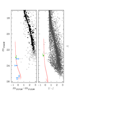
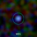
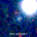
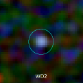
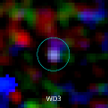
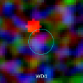
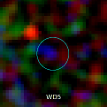
Figure 16: Left panels show the $m_{\rm F090W}$ versus $(m_{\rm F070W}-m_{\rm F150W})$ and the $V$ versus $(V-I)$ CMDs of NGC 2506 obtained with the NIRCam@JWST and WFC@INT data sets. In the leftmost panel the grey and black points are stars that passed the selection and membership criteria, respectively. Green and azure squares represent the sources that, based on their membership and/or position on the CMDs, may be considered candidate WDs. In red are reported the 2 Gyr WD isochrones; dotted lines represent the isochrone boundaries considering the errors on the distance modulus and reddening. The finding charts of the candidate WDs are shown in the right panels. The field of view of JWST finding charts is $1.2\times 1.2$ arcsec², while the WFC finding chart is $6.5\times 6.5$ arcsec². Sources WD1, WD2, and WD3 appear as point-like stars, while WD4 and WD5 should be noisy peaks.

Table 4: Candidate WDs identified in NGC 2506

WD	$\alpha$	$\delta$	$m_{\rm F090W}$	$m_{\rm F070W}$	$m_{\rm F150W}$
	(deg.)	(deg.)
1	120.0166589	$-$10.8069775	$22.95\pm 0.05$	$22.79\pm 0.06$	$23.16\pm 0.01$
2	120.0102662	$-$10.8069270	$23.13\pm 0.06$	$22.94\pm 0.03$	$23.18\pm 0.15$
3	120.0571064	$-$10.7940803	$23.98\pm 0.02$	$23.50\pm 0.06$	$23.75\pm 0.13$
4	120.0296222	$-$10.7618422	$25.40\pm 0.04$	$25.11\pm 0.03$	$24.94\pm 0.02$
5	120.0466738	$-$10.8187002	$25.52\pm 0.01$	$24.71\pm 0.14$	$24.88\pm 0.10$

5.2 Mass Functions and total mass

We computed the luminosity functions (LFs) of MS stars counting stars in magnitude intervals that contain an equal number of stars and using both the Gaia and the JWST catalogue, and then we converted the LFs to mass functions (MFs) by adopting the mass-luminosity relation from the BaSTI-IAC isochrones.

As shown in panels (a) and (b) of Fig. 15, thanks to the synergy between Gaia and JWST data, we are able to cover a mass range from $\sim 0.1~{}M_{\odot}$ to $\sim 1.4~{}M_{\odot}$, encompassing the very low mass stars and extending up to the main sequence turn-off.

Panels (c) and (d) of Fig. 15 show the MFs obtained with the Gaia catalogue. They are also reported in Table 3. To calculate the LFs, we accounted for the contribution of each star in a given magnitude interval weighted by its MP to be a cluster member, as already done in the previous sections. We focused on MS stars with magnitudes between $G_{\rm RP}=14.50$ and $G_{\rm RP}=18.25$, corresponding to a mass interval between $M=0.74~{}M_{\odot}$ and $M=1.46~{}M_{\odot}$. Initially, we considered the present day MF as described by the equation:

$$\frac{{\rm d}N}{{\rm d}M}\propto M^{\alpha}$$ (9)

which is a straight line in the logarithmic form:

$$\log{\left(\frac{{\rm d}N}{{\rm d}M}\right)}=\beta+{\alpha}\log{(M)}$$ (10)

Panel (c) illustrates the MFs calculated in three radial bins containing an equal number of MS stars. We fitted a straight line to each MF within each radial bin using a weighted least square fit, with the inverse square of the MF errors serving as the weights. We obtained three estimates of the present-day local MF. For the inner region ($R<3.85$ arcmin), we derived a slope $\alpha=-0.99\pm 0.25$; in the middle region ($3.85\leq R<8.33$ arcmin) the slope is $\alpha=-2.22\pm 0.19$. Finally, for the outermost region ($8.33\leq R<33.00$ arcmin) the slope measured is $\alpha=-2.80\pm 0.24$. We also calculated the slope of the MF using a single interval ($0.00\leq R<33.00$ arcmin), and found $\alpha=-2.04\pm 0.14$; i.e., a proxy for the present-day global mass function. The change in slope with radial distance from the centre is attributed to the mass segregation effect resulting from the cluster dynamical evolution, as previously noted by Lee et al. (2013) and Rangwal et al. (2019).

To determine the contribution to the cluster mass from stars with $M\geq 0.74M_{\odot}$, we utilised the MF shown in panel (d) of Fig.15. Our analysis yielded $M_{\rm cluster}[0.74M_{\odot}\leq M\leq 1.46M_{\odot}]=2077\pm 67~{}M_{\odot}$. We also performed the same computation by using the three MFs shown in panel (c) of Fig. 15: summing the single total mass contributions in each radial bin, we obtained a mass $M_{\rm cluster}[0.74M_{\odot}\leq M\leq 1.46M_{\odot}]=2054\pm 69~{}M_{\odot}$. This result aligns with the previously determined value, confirming that mass segregation does not significantly impact the estimate of the cluster mass obtained by integrating the global mass function rather than using local mass functions.

We calculated the MFs in the area covered by the JWST dataset, spanning approximately 20 arcmin² between 0.24 arcmin and 4.61 arcmin from the cluster centre. The results are presented in Table 3 and in panel (e) of Fig. 15. First, we calculated the MF for stars with masses between $0.74~{}M_{\odot}$ and $1.46~{}M_{\odot}$ using Gaia DR3 following the procedure previously described (black points). For the JWST data, we adopted two different approaches to compute the MFs. The first approach involved the use of proper motions and was limited to stars with masses between $0.37~{}M_{\odot}$ and $0.93~{}M_{\odot}$ (as ground-based INT images do not reach magnitudes as faint as the JWST data, see Sect. 2.4). In this case, we followed a similar procedure as for the Gaia data, weighting the MFs with MPs and correcting for completeness (blue points in panel (e) of Fig. 15). To extend the MF to lower masses, we performed a statistical decontamination of the LFs to account for the contribution of field stars. We selected stars in the Gaia catalogue located in the JWST region with magnitudes $16.5\leq G_{\rm RP}\leq 17.5$, corresponding to a mass range between $0.84~{}M_{\odot}$ and $1.03~{}M_{\odot}$ on the MS. Within this mass interval, which corresponds to the magnitude range $15.67\leq m_{\rm F277W}\leq 16.42$, we calculated the weighted sum of the number of stars considering the non-membership probabilities as weights. Next, we determined the mean number of expected field stars per unit F277W magnitude by dividing the sum by 0.75 (the F277W magnitude range). We obtained a contamination factor of 22.8 stars/F277W magnitude. We subtracted this value appropriately from the number of stars counted in each magnitude interval used to construct the LFs. The resulting MF is represented by orange squares in panel (e) of Fig. 15. Since the total MF does not conform to a single power law, we fitted three straight lines to the ${\rm d}N/{\rm d}M$ vs. $M$ distribution in different mass intervals: for the mass range $0.8M_{\odot}<M\leq 1.4M_{\odot}$, we obtained a power-law exponent $\alpha=-1.74\pm 0.22$; for masses $0.3M_{\odot}<M\leq 0.8M_{\odot}$, the best-fit was obtained for $\alpha=-0.82\pm 0.17$; finally, in the low-mass regime $0.1M_{\odot}\leq M\leq 0.3M_{\odot}$ we measured $\alpha=-0.18\pm 0.10$.

We computed the total mass for stars in the JWST region with masses in the interval $0.10~{}M_{\odot}\leq M\leq 1.46~{}M_{\odot}$, and obtained $M_{\rm cluster,JWST}[0.10M_{\odot}\leq M\leq 1.46M_{\odot}]=601\pm 21~{}M_{\odot}$, of which $\sim 50~{}\%$ is due to stars with masses between $0.74~{}M_{\odot}$ and $1.46~{}M_{\odot}$. We found that the combined MF obtained from JWST and Gaia data can be well described by the logistic function:

$$\log{\left(\frac{{\rm d}N}{{\rm d}M}\right)}=\frac{c}{1+a\exp{(-b\log{M})}}$$ (11)

as shown in panel (f) of Fig. 15. The best-fitting parameters were determined as $a=0.231\pm 0.020$, $b=-3.436\pm 0.531$, and $c=3.290\pm 0.048$. By integrating this function, we obtained a total mass $M_{\rm cluster,JWST}[0.10M_{\odot}\leq M\leq 1.46M_{\odot}]=614\pm 77~{}M_{\odot}$, in agreement with the value found by using three power laws.

We used this just derived information on the MFs within the JWST region to obtain an estimate for the present-day total mass of the stellar cluster NGC 2506 based only on stars with masses ranging between 0.1 and 1.46 $M_{\odot}$. In this calculation we assume that the relative number of stars of different mass in the entire cluster is the same as that observed within the annulus covered by JWST, i.e., within $0.24\leq R\leq 4.61$ arcmin. We then calculated the total mass of the cluster in this annulus and scaled it to the total region occupied by the cluster. We obtained $M_{\rm cluster,0.24-4.61arcmin}=M_{\rm cluster,JWST}\times A({\rm annulus})/A({\rm JWST})=2021\pm 150~{}M_{\odot}$ where $A({\rm annulus})/A({\rm JWST})$ is the ratio between the area of the annulus and the area covered by JWST observations. We then calculated the cluster mass in an annulus between $4.61\leq R\leq 33.00$ arcmin using stars with masses between 0.74 and 1.46 $M_{\odot}$ included in the Gaia catalogue; we found a mass of $1223\pm 47~{}M_{\odot}$, which is $\sim 59$ % of the total mass previously calculated for this mass range. Supposing that the mass distribution is the same in the two radial bins, we calculated a total mass equal to $\sim 5863~{}M_{\odot}$. This must be considered as a lower limit of the present-day total mass because it does not take into account, i.e., of the evolved stars (giant stars, white dwarfs, etc.), of stars with masses $<0.1~{}M_{\odot}$, and of the brown dwarfs.

6 White dwarfs in NGC 2506

We investigated the presence of white dwarfs (WDs) in the JWST CMDs of NGC 2506 using the bluer, higher SNR filters, i.e. F070W, F090W, and F150W, where WDs are expected to be more prominent. The results are presented in Fig.16 and Table 4. The leftmost panel shows the $m_{\rm F090W}$ versus $(m_{\rm F070W}-m_{\rm F150W})$ CMD of the stars that passed the selection and membership criteria in grey and black, respectively. The isochrone of WDs with an age of 2 Gyr is depicted in red. This WD isochrone has been calculated as described in Griggio et al. (2023a) using the BaSTI-IAC WD cooling models by Salaris et al. (2022) for progenitors with initial [M/H]=$-$0.40. We obtain essentially the same isochrone if we use cooling models from progenitors with [M/H]=$-$0.20, the other metallicity in the WD BaSTI-IAC database close to the cluster [M/H]. The green square shows the only WD with a high-membership probability (92.1 %), as consistently located along the WD cooling sequence. According to the initial-final mass relation adopted in the calculation of the isochrone (Cummings et al., 2018) the mass of this WD is $\sim$0.62$M_{\odot}$.

This same star (WD1, $V=22.74\pm 0.08$, $I=23.07\pm 0.03$) is also displayed in the $V$ versus $(V-I)$ CMD obtained with the WFC@INT data set, where it also closely matches the WD isochrone within the measurement errors. The azure squares in the leftmost panel represent other sources near the WD isochrone but without proper motion measurements, which should be considered as candidate WDs. A suitable astrometric second epoch appears as the most efficient way to confirm as members these WD candidates. We visually examined these five sources using three-colour stacked images obtained with the same filters employed for the CMDs. The results are presented in the right panels: candidate WDs 1, 2, and 3 appear as clear point-like sources in both the JWST and WFC@INT images. On the other hand, WD4 and WD5 likely correspond to noisy peaks that passed the selection criteria. However, with deeper data collected by either HST or JWST in the future, this ambiguity may be resolved.

7 Summary

In this work we have exploited JWST non-proprietary calibration data to: (i) derive accurate effective PSFs for ten filters (8 wide + 2 medium), spanning a wavelength interval from 0.7 $\mu$m to 4.5 $\mu$m; (ii) extract high-precision photometry and astrometry from "shallow" NIRCam images for stars located in the region that encompasses a portion of the 2 Gyr open cluster NGC 2506; (iii) calculate the proper motions for MS stars with masses $\gtrsim 0.3~{}M_{\odot}$ by adopting ground-based data collected with the INT a taking advantage of the large temporal baseline ($\sim 18.8$ years) between JWST and INT data; (iv) carry-out an in-depth analysis of the cluster properties by leveraging the synergy between JWST data and the Gaia DR3 catalogue.

We have calculated the radial stellar density profile by using the Gaia DR3 catalogue, fitted with a King profile. From the fitting, we derive the central stellar density ($k_{0}=28.1\pm 0.9$ stars/arcmin²), the core radius ($r_{\rm c}=2.60\pm 0.05$ arcmin), and the tidal radius ($r_{\rm t}=33.0\pm 4.3$ arcmin).

From the combination of JWST and Gaia DR3 data, we calculated the fraction of MS binaries with mass ratio $q\geq 0.6$, equal to $\sim 23$ %. This synergy allowed us to extend the study of the MS binary fraction down to $\sim 0.4~{}M_{\odot}$, well below the Gaia limit ($\sim 0.8~{}M_{\odot}$). Our findings reveal no dependence of the binary fraction on the primary mass within a mass range between $0.44M_{\odot}$ and $1.13M_{\odot}$. However, we observed a hint of a radial trend in the radial distribution of the MS binary fraction between the cluster centre and approximately $2r_{\rm c}$.

Similarly, by leveraging the synergy between JWST and Gaia DR3, we computed MFs of MS stars within the mass interval from $\sim 0.10M_{\odot}$ to $\sim 1.45M_{\odot}$. First, we examined the MFs using solely Gaia DR3 data. Our analysis confirmed the influence of mass segregation on the MFs calculated in various radial bins for masses ranging from $\sim 0.7~{}M_{\odot}$ to $\sim 1.4~{}M_{\odot}$. By integrating these mass functions, we determined that the total mass of stars within the range from $0.74~{}M_{\odot}$ to $1.46~{}M_{\odot}$ is $\sim 2065~{}M_{\odot}$. We then focused on the region covered by JWST data ($0.24\leq R\leq 4.61$ arcmin). We found that the MF for stars with masses between $\sim 0.1~{}M_{\odot}$ and $\sim 1.4~{}M_{\odot}$ is well represented by a logistic function. By calculating the total mass of stars within this region ($\sim 600M_{\odot}$) and assuming a homogeneous mass distribution, we estimated the total mass within $R\leq 4.61$ arcmin to be $\sim 2021~{}M_{\odot}$. We used this number to put a lower limit on the total mass of the cluster, which is estimated to be about $6000~{}M_{\odot}$.

Finally, using the bluest JWST available filters, we identified five candidate white dwarfs. Among them, WD1 stands out as the strongest candidate due to its relatively high brightness, the high membership probability and alignment with the theoretical 2 Gyr white dwarf cooling sequence (also on the ground-based CMD). A preliminary estimate suggests that the mass of WD1 is $\sim 0.62~{}M_{\odot}$. However, to resolve the ambiguity surrounding these candidates, it will be necessary to acquire new, deeper data using instruments such as HST or JWST.

As a byproduct of this work, we release the derived ePSFs and the JWST catalogues and atlases of NGC 2506 (see Appendix B).

This study has demonstrated the potential of using JWST’s publicly available calibration images in combination with the Gaia catalogue, to conduct a pioneering multi-band analysis of stellar populations in open clusters within the IR wavelength range. With a minimum effort of observing time, we were able to probe the faint end of the MS in this peculiar, old, and distant open cluster. Future NIRCam deeper observations of different open clusters, spanning multiple years, will enable us to easily explore their brown dwarf sequence, study the mass functions and evaporation effects of low-mass stars ($<0.2~{}M_{\odot}$), the internal kinematic via proper-motions, as well as investigate their white dwarf cooling sequences, advancing our understanding of stellar populations in star clusters and shedding light on the diverse phenomena within these systems.

Data Availability

The data underlying this article are publicly available in the Mikulski Archive for Space Telescopes at https://mast.stsci.edu/. The catalogues underlying this work are available in the online supplementary material of the article.

Appendix A PSF variations across the detectors

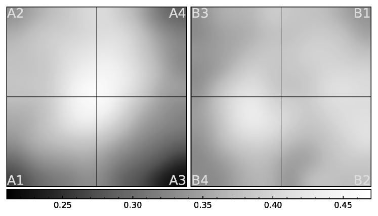
Figure 17: Variation across the detector of the peak of the PSF in F070W filter.

Given the great level of accuracy of our here-derived second-generation PSFs, significantly improved (if compared with the PSFs from Paper I) thanks to the available geometric distortion corrections (derived only in Paper II), we can now provide the community with an independent determination of the average spatial properties of the PSFs. Indeed, it would be particularly useful to know precisely where to place a target in order to obtain the highest possible angular resolution with NIRCam@JWST observations. Given the dependency of the angular resolution on the wavelength for a diffraction-limited ‘optical’ (actually, IR) system, the bluest filters are those expected to show the maxima spatial variations, as they would amplify relative differences. Furthermore, the under-sampled nature of NIRCam PSFs of bluest filters makes the PSFs of the filters F070W/F090W/F115W the hardest PSFs to solve for.

In Fig. 17, we show the spatial determination of PSFs’s peaks in the most undersampled filter F070W, obtained by interpolating the 5$\times$5 perturbed PSF arrays of all the images. PSFs values are normalised to 1 within an area of 5.25$\times$5.25 physical pixels. So a value of 0.47 meaning that the central pixels, of a source centred at the centre of a pixels, contain 47% of the normalised flux. Figure 17 reveals that Module A (on the left) has a sharpest ’sweet spot’ in a region between the four detectors, where targets that need the highest angular resolution (FWHM$\sim$35 mas, containing 47% of the light in its central pixel) should be placed. Also Module B shows a slightly less-peaked sweet spot than Module A, and relatively off-centre, mainly within B4.

These differences between PSFs at different spatial position within NIRCam field of view, become less and less important moving to redder wavelengths.

Appendix B Electronic Material

The catalogues of NGC 2506 extracted in this work will be released as supporting material to this paper. We will release two catalogues, one for each field of view covered by Module A and B, that contain information on the position of the stars, the VEGAmag calibrated magnitudes in the 10 JWST filters, the quality parameters described in Sect. 2.2.1, the quality flag of the selections described in Sect. 2.2.1; the proper motions and the membership probabilities, and the completeness associated to each star. We will also make publicly available the ePSFs and the stacked images in each filter derived in this work at the website: https://web.oapd.inaf.it/bedin/files/PAPERs_eMATERIALs/JWST/. At the same website we will upload the NGC 2506 catalogues.

References

- Anderson (2016) Anderson J., 2016, Empirical Models for the WFC3/IR PSF, Instrument Science Report WFC3 2016-12, 42 pages
- Anderson & King (2000) Anderson J., King I. R., 2000, PASP, 112, 1360
- Anderson & King (2004) Anderson J., King I. R., 2004, Multi-filter PSFs and Distortion Corrections for the HRC, Instrument Science Report ACS 2004-15, 51 pages
- Anderson & King (2006) Anderson J., King I. R., 2006, PSFs, Photometry, and Astronomy for the ACS/WFC, Instrument Science Report ACS 2006-01, 34 pages
- Anderson et al. (2006) Anderson J., Bedin L. R., Piotto G., Yadav R. S., Bellini A., 2006, A&A, 454, 1029
- Anderson et al. (2008) Anderson J., et al., 2008, AJ, 135, 2114
- Anderson et al. (2015) Anderson J., Bourque M., Sahu K., Sabbit E., Viana A., 2015, A Study of the Time Variability of the PSF in F606W Images taken with the WFC3/UVIS, Instrument Science Report WFC3 2015-08, 19 pages
- Anthony-Twarog et al. (2005) Anthony-Twarog B. J., Atwell J., Twarog B. A., 2005, AJ, 129, 872
- Anthony-Twarog et al. (2006) Anthony-Twarog B. J., Tanner D., Cracraft M., Twarog B. A., 2006, AJ, 131, 461
- Anthony-Twarog et al. (2016) Anthony-Twarog B. J., Deliyannis C. P., Twarog B. A., 2016, AJ, 152, 192
- Anthony-Twarog et al. (2018) Anthony-Twarog B. J., Lee-Brown D. B., Deliyannis C. P., Twarog B. A., 2018, AJ, 155, 138
- Arentoft et al. (2007) Arentoft T., et al., 2007, A&A, 465, 965
- Bailer-Jones et al. (2021) Bailer-Jones C. A. L., Rybizki J., Fouesneau M., Demleitner M., Andrae R., 2021, AJ, 161, 147
- Bedin et al. (2003) Bedin L. R., Piotto G., King I. R., Anderson J., 2003, AJ, 126, 247
- Bedin et al. (2004) Bedin L. R., Piotto G., Anderson J., Cassisi S., King I. R., Momany Y., Carraro G., 2004, ApJ, 605, L125
- Bedin et al. (2008) Bedin L. R., King I. R., Anderson J., Piotto G., Salaris M., Cassisi S., Serenelli A., 2008, ApJ, 678, 1279
- Bellini et al. (2010) Bellini A., et al., 2010, A&A, 513, A50
- Bellini et al. (2013) Bellini A., Anderson J., Salaris M., Cassisi S., Bedin L. R., Piotto G., Bergeron P., 2013, ApJ, 769, L32
- Bellini et al. (2017) Bellini A., Anderson J., Bedin L. R., King I. R., van der Marel R. P., Piotto G., Cool A., 2017, ApJ, 842, 6
- Boubert & Everall (2020) Boubert D., Everall A., 2020, MNRAS, 497, 4246
- Cantat-Gaudin & Anders (2020) Cantat-Gaudin T., Anders F., 2020, A&A, 633, A99
- Carretta et al. (2004) Carretta E., Bragaglia A., Gratton R. G., Tosi M., 2004, A&A, 422, 951
- Chambers et al. (2016) Chambers K. C., et al., 2016, arXiv e-prints, p. arXiv:1612.05560
- Cordoni et al. (2023) Cordoni G., et al., 2023, A&A, 672, A29
- Cummings et al. (2018) Cummings J. D., Kalirai J. S., Tremblay P. E., Ramirez-Ruiz E., Choi J., 2018, ApJ, 866, 21
- Dieball et al. (2016) Dieball A., Bedin L. R., Knigge C., Rich R. M., Allard F., Dotter A., Richer H., Zurek D., 2016, ApJ, 817, 48
- Everall & Boubert (2022) Everall A., Boubert D., 2022, MNRAS, 509, 6205
- Feinstein et al. (2023) Feinstein A. D., et al., 2023, Nature, 614, 670
- Gaia Collaboration et al. (2021) Gaia Collaboration et al., 2021, A&A, 649, A1
- Gaia Collaboration et al. (2022) Gaia Collaboration et al., 2022, arXiv e-prints, p. arXiv:2208.00211
- Gao (2020) Gao X., 2020, ApJ, 894, 48
- Gardner et al. (2023) Gardner J. P., et al., 2023, PASP, 135, 068001
- Griggio & Bedin (2022) Griggio M., Bedin L. R., 2022, MNRAS, 511, 4702
- Griggio et al. (2022) Griggio M., et al., 2022, MNRAS, 515, 1841
- Griggio et al. (2023a) Griggio M., Salaris M., Nardiello D., Bedin L. R., Cassisi S., Anderson J., 2023a, arXiv e-prints, p. arXiv:2306.09845
- Griggio et al. (2023b) Griggio M., Nardiello D., Bedin L. R., 2023b, Astronomische Nachrichten, 344, e20230019
- Hidalgo et al. (2018) Hidalgo S. L., et al., 2018, ApJ, 856, 125
- King (1962) King I., 1962, AJ, 67, 471
- King et al. (2005) King I. R., Bedin L. R., Piotto G., Cassisi S., Anderson J., 2005, AJ, 130, 626
- Knudstrup et al. (2020) Knudstrup E., et al., 2020, MNRAS, 499, 1312
- Lee et al. (2013) Lee S. H., Kang Y. W., Ann H. B., 2013, MNRAS, 432, 1672
- Libralato et al. (2014) Libralato M., Bellini A., Bedin L. R., Piotto G., Platais I., Kissler-Patig M., Milone A. P., 2014, A&A, 563, A80
- Libralato et al. (2016a) Libralato M., Bedin L. R., Nardiello D., Piotto G., 2016a, MNRAS, 456, 1137
- Libralato et al. (2016b) Libralato M., et al., 2016b, MNRAS, 463, 1780
- Libralato et al. (2023) Libralato M., et al., 2023, arXiv e-prints, p. arXiv:2303.00009
- Magnier et al. (2020) Magnier E. A., et al., 2020, ApJS, 251, 3
- McClure et al. (1981) McClure R. D., Twarog B. A., Forrester W. T., 1981, ApJ, 243, 841
- Mikolaitis et al. (2011) Mikolaitis Š., Tautvaišienė G., Gratton R., Bragaglia A., Carretta E., 2011, MNRAS, 416, 1092
- Milone et al. (2012) Milone A. P., et al., 2012, A&A, 540, A16
- Milone et al. (2016) Milone A. P., et al., 2016, MNRAS, 455, 3009
- Milone et al. (2019) Milone A. P., et al., 2019, MNRAS, 484, 4046
- Naidu et al. (2022) Naidu R. P., et al., 2022, ApJ, 940, L14
- Nardiello et al. (2015) Nardiello D., Milone A. P., Piotto G., Marino A. F., Bellini A., Cassisi S., 2015, A&A, 573, A70
- Nardiello et al. (2016a) Nardiello D., Libralato M., Bedin L. R., Piotto G., Ochner P., Cunial A., Borsato L., Granata V., 2016a, MNRAS, 455, 2337
- Nardiello et al. (2016b) Nardiello D., Libralato M., Bedin L. R., Piotto G., Borsato L., Granata V., Malavolta L., Nascimbeni V., 2016b, MNRAS, 463, 1831
- Nardiello et al. (2018a) Nardiello D., et al., 2018a, MNRAS, 477, 2004
- Nardiello et al. (2018b) Nardiello D., et al., 2018b, MNRAS, 481, 3382
- Nardiello et al. (2019) Nardiello D., Piotto G., Milone A. P., Rich R. M., Cassisi S., Bedin L. R., Bellini A., Renzini A., 2019, MNRAS, 485, 3076
- Nardiello et al. (2022) Nardiello D., Bedin L. R., Burgasser A., Salaris M., Cassisi S., Griggio M., Scalco M., 2022, MNRAS, 517, 484
- Nardiello et al. (2023) Nardiello D., Griggio M., Bedin L. R., 2023, MNRAS, 521, L39
- Netopil et al. (2016) Netopil M., Paunzen E., Heiter U., Soubiran C., 2016, A&A, 585, A150
- Panthi et al. (2022) Panthi A., Vaidya K., Jadhav V., Rao K. K., Subramaniam A., Agarwal M., Pandey S., 2022, MNRAS, 516, 5318
- Paris et al. (2023) Paris D., et al., 2023, arXiv e-prints, p. arXiv:2301.02179
- Pietrinferni et al. (2021) Pietrinferni A., et al., 2021, ApJ, 908, 102
- Piotto et al. (2007) Piotto G., et al., 2007, ApJ, 661, L53
- Piotto et al. (2015) Piotto G., et al., 2015, AJ, 149, 91
- Rangwal et al. (2019) Rangwal G., Yadav R. K. S., Durgapal A., Bisht D., Nardiello D., 2019, MNRAS, 490, 1383
- Richer et al. (2008) Richer H. B., et al., 2008, AJ, 135, 2141
- Rieke et al. (2023) Rieke M. J., et al., 2023, PASP, 135, 028001
- Sabbi et al. (2016) Sabbi E., et al., 2016, ApJS, 222, 11
- Salaris et al. (2022) Salaris M., Cassisi S., Pietrinferni A., Hidalgo S., 2022, MNRAS, 509, 5197
- Scalco et al. (2021) Scalco M., et al., 2021, MNRAS, 505, 3549
- Schlafly & Finkbeiner (2011) Schlafly E. F., Finkbeiner D. P., 2011, ApJ, 737, 103
- Schlegel et al. (1998) Schlegel D. J., Finkbeiner D. P., Davis M., 1998, ApJ, 500, 525
- Stetson (2000) Stetson P. B., 2000, PASP, 112, 925
- Tarricq et al. (2021) Tarricq Y., et al., 2021, A&A, 647, A19
- Waters et al. (2020) Waters C. Z., et al., 2020, ApJS, 251, 4
- Ziliotto et al. (2023) Ziliotto T., et al., 2023, arXiv e-prints, p. arXiv:2304.06026
- de Pater et al. (2022) de Pater I., et al., 2022, in AAS/Division for Planetary Sciences Meeting Abstracts. p. 306.07