Slow dissipation and spreading in disordered classical systems:
A direct comparison between numerics and mathematical bounds

Abstract

We study the breakdown of Anderson localization in the one-dimensional nonlinear Klein-Gordon chain, a prototypical example of a disordered classical many-body system. A series of numerical works indicate that an initially localized wave packet spreads polynomially in time, while analytical studies rather suggest a much slower spreading. Here, we focus on the decorrelation time in equilibrium. On the one hand, we provide a mathematical theorem establishing that this time is larger than any inverse power law in the effective anharmonicity parameter $\lambda$, and on the other hand our numerics show that it follows a power law for a broad range of values of $\lambda$. This numerical behavior is fully consistent with the power law observed numerically in spreading experiments, and we conclude that the state-of-the-art numerics may well be unable to capture the long-time behavior of such classical disordered systems.

Introduction — Since at least two decades there has been vivid interest in the dynamical behavior of certain disordered classical interacting systems, like the nonlinear discrete Schrödinger equation (NLS) or the nonlinear Klein-Gordon chain (KG). These systems are characterized by the feature that, when the anharmonicity is set to zero but the disorder strength remains finite, their eigenmodes are spatially localized by Anderson localization [1]. The natural question is then what happens at small but finite anharmonicity, where there is an evident competition between the localization of the linear system on the one hand, and chaoticity and dissipation brought about by anharmonicity on the other hand.

We are in particular motivated by previous compelling numerical work on spreading of initially localized wave packets in such systems [2, 3, 4, 5, 6, 7, 8, 9, 10, 11, 12, 13, 14, 15, 16]. In these works, it was found that the width $w$ of the evolved wave packet grows as $w\varpropto t^{1/6}$ for several chains with a quartic on-site anharmonicity, including KG and NLS. These numerical findings are however at odds with a vast body of theoretical work [17, 18, 19, 20, 21, 22, 23, 24, 25, 26, 27, 28], supported by some numerics as [29, 30]. These works suggest that dissipative effects are non-perturbatively small in the effective anharmonicity $\lambda$, to be defined below. In particular, on the basis of Hamiltonian perturbation theory similar to that used in the proof of the KAM theorem, it is predicted that the thermal conductivity (or, for that matter, any other measure of dissipation) vanishes faster than any power of $\lambda$, which suggests a much slower spreading of the wavepacket, namely $w\varpropto(\log t)^{\alpha}$ for some power $\alpha$.

In the light of this discrepancy, the few pre-existing mathematical results like [20, 22, 28, 26] do not offer solace. Indeed, first, they do not apply to the system at hand, since the Anderson insulator at $\lambda=0$ is replaced in these works by a set of independent oscillators, known as the atomic limit of the system. And second, with the exception of [20], they do not constrain the long-time limit of spreading of wave packets.

In this letter we report on work that in our view settles this conundrum: We provide for the first time a direct comparison between numerical observations and mathematical bounds for the KG chain. As an alternative to the speed of spreading or the diffusion constant, we focus on the decorrelation time in thermal equilibrium as it is more accessible to a proper mathematical treatment and to numerics. On the one hand, we prove a mathematical theorem stating that this time is larger than any polynomial in $\lambda$ as $\lambda\to 0$, see Figure 1. On the other hand, we perform numerical analysis, for precisely the same system and the same observable, and we find a broad range of values of $\lambda$ where the decorrelation time scales as $\lambda^{-4}$, which is consistent with the diffusion constant scaling as $\lambda^{4}$ and with the behavior $w\varpropto t^{1/6}$ for the evolution of the width of a wave packet.

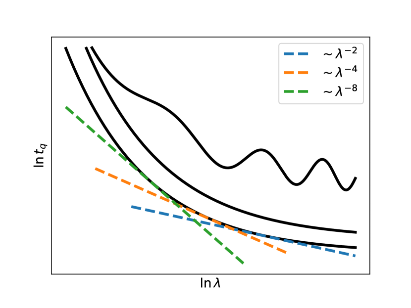
Figure 1: Mathematical constraints on the decorrelation time are shown as straight lines on this plot. The true curve has to lie above all these lines (like the 3 displayed black curves).

We conclude from our results that the KG chain is asymptotically many-body localized as $\lambda\to 0$. By this term, we mean that the onset of dissipation is a fully non-perturbative phenomenon [25, 28, 31, 27, 32], implying in particular that decorrelation times grow faster than any power law in $\lambda$. Our findings also strongly suggest that the spreading of an initially localized wavepacket is slower than any polynomial in time, and that the simulation time should be considerably extended in order to observe a behavior that deviate significantly from the scaling $w\varpropto t^{1/6}$.

Decorrelation times — The nonlinear Klein-Gordon Hamiltonian is

$$H=\sum_{i=1}^{L}\frac{p_{i}^{2}}{2}+\frac{\omega^{2}_{i}q_{i}^{2}}{2}+\frac{(q_{i+1}-q_{i})^{2}}{2W}+\gamma\frac{q_{i}^{4}}{4},$$

where the momenta $p_{i}$ are canonically conjugated to the positions $q_{i}$, where $\omega^{2}_{i}$ are independent random variables, uniformly distributed in the interval $[1/2,3/2]$, and where we assume periodic boundary conditions $q_{L+1}=q_{1}$. At $\gamma=0$, this Hamiltonian is quadratic and it can be recast in action-angle coordinates $(I_{k},\phi_{k})$ as

$$H_{0}=\sum_{k}\nu_{k}I_{k}=\tfrac{1}{2}\sum_{k}(\langle\psi_{k},p\rangle^{2}+\nu_{k}^{2}\langle\psi_{k},q\rangle^{2}).$$ (1)

Here $\langle\cdot,\cdot\rangle$ denotes the usual scalar product in $\mathbb{R}^{L}$ and $\nu_{k}^{2},\psi_{k}$ are eigenvalues and eigenfunctions (normalized as $\langle\psi_{k},\psi_{k}\rangle=1$) of the associated discrete Schrödinger operator $\mathcal{H}$:

$$\mathcal{H}f(i)=\frac{1}{W}(f(i+1)+f(i-1)-2f(i))+\omega_{i}^{2}f(i).$$

Since this Schrödinger operator has a disordered potential and the spatial dimension is $1$, its eigenstates are Anderson localized [1, 33, 34, 35], i.e. they are exponentially localized in space around localization centers. As a consequence, the corresponding actions $I_{k}$ are exponentially localized as well. An initially localized wavepacket will hence remain localized at all times, i.e.  the width $w(t)$ is bounded above as $t\to\infty$, almost surely with respect to the disorder. At nonzero $\gamma$, $H$ contains also a quartic part in square root of the actions $I_{j}$, dependent on the angles, so that $I_{j}$ are no longer conserved. For a generic observable $X$, we introduce the decorrelation indicator

$$\eta_{X}(t)=\frac{1}{2}\frac{\langle(X(t)-X(0))^{2}\rangle}{\langle X(t)^{2}\rangle-\langle X(t)\rangle^{2}}.$$

with $\langle\cdot\rangle$ the thermal average at some fixed temperature $T$. A scaling argument shows that $\eta_{X}(\cdot)$ depends on the parameters $(\gamma,T)$ only via the effective anharmonicity

$$\lambda=\gamma T.$$

If the dynamics is thermalizing or more precisely mixing, then we expect that $\eta_{X}(t)$ rises from $0$ to $1$ as $t\to\infty$, up to small corrections due to the difference between the canonical and microcanonical ensembles, vanishing as $1/L$ as $L\to\infty$.

We choose $X=X_{k}=\nu_{k}I_{k}$ and we average over $L=80$ modes $k$ (our system size is $L=80$ sites) and over disorder, i.e. over the variables $\omega_{i}^{2}$, obtaining the quantity

$$\eta(t)=\overline{\frac{1}{L}\sum_{k=1}^{L}\eta_{X_{k}}(t)}^{\,\omega}.$$

Figure 2 shows our best estimator for $\eta(t)$ for several values of $\lambda$, see Supplementary Material (SM).

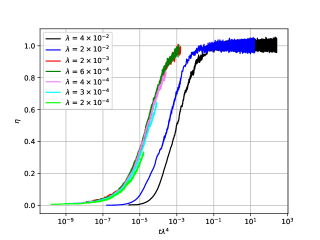
Figure 2: The decorrelation $\eta(t)$ as a function of rescaled time $\lambda^{4}t$. With this rescaling, we observe collapse of decorrelation profiles for small anharmonicities $\lambda$.

We define the decorrelation time $\tau$ as the time at which $\eta$ reaches a fixed value $\eta_{0}$. We plot it for two different values of $\eta_{0}$ in Figure 3.

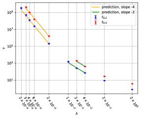
Figure 3: The decorrelation time extraced from Figure 2, with $\eta_{0}=0.2$ and $\eta_{0}=0.5$. We indicated by straight lines the regime for which $\tau\propto\lambda^{-4}$, and a short regime for which $\tau\propto\lambda^{-2}$.

Both figures 2 and 3 show the existence of scaling $\tau\propto\lambda^{-4}$ for small $\lambda$.

Range of validity for scaling — Both figures 2 and 3 give a slight hint that the decorrelation time starts increasing faster than $\lambda^{-4}$ at small $\lambda$ but they also confirm that the $\lambda^{-4}$ scaling is valid for a range of anharmonicities that spans at least 1 or even 1,5 decades. We can compare the data from Figures 2 and 3 to the numerics on spreading wavepackets by assuming that local thermal equilibrium holds inside the packet (we comment on this later): When the packet has a width $w$, the typical temperature inside the packet is of order $E_{0}/w$ with $E_{0}$ the total energy of the packet, see SM for precise calculations. If we assume the scaling $w\propto t^{1/6}$ to hold for times in the range $[t_{0},t_{1}]$, then that scaling holds for a corresponding range of temperatures $[T_{0},T_{1}]$ with $T_{1}/T_{0}=(t_{1}/t_{0})^{1/6}$. Looked upon differently, this means that the validity of the scaling regime for $1,5$ decades correspond to its validity for $9$ decades in time! Indeed, in [4, 5], the scaling $w\propto t^{1/6}$ was observed for $6-8$ decades, which is hence perfectly consistent with out results. In [14], it was observed for 12 decades in a related, though different, model. While a direct comparison with our numerics is difficult due to the differences between the models, it is important to realize that here as well, the relevant parameter is the effective anharmonicity reached when the packet has maximally spread out, see SM for details. Note that the above reasoning does not rely on any intrinsic connection between the $w\propto t^{1/6}$ law and the $\tau\propto\lambda^{-4}$ law. We will describe later that there is however such a connection though this is actually not crucial for our argument.

Finally, we can compare our numerics with the numerics on spreading of wave packets in the following way. Since we see a hint of a deviation from the $\tau\propto\lambda^{-4}$ law, one could ask how hard it would be to probe the same nonlinearities as we do in a spreading experiments. It is harder because spreading numerics needs a larger volume than our decorrelation numerics. More concretely, to see our smallest nonlinearity in the setup [4, 5], we would have to simulate the system $250$ times longer than done in [4, 5], (assuming that the spreading does not slow down compared to the $t^{1/6}$ law), see Section VI of SM.

A rigorous result — In the companion paper [36], we have proven the following mathematical result. Let us fix an arbitrary threshold value $0<q<1$ for the decorrelation parameter $\eta$, as in Figure 3. Let $t_{q}$ be the smallest positive time such that $\eta(t)\geq q$ (this time exists by continuity). Then

Theorem 1 (Slow decorrelation).

For any integer $n$, there is a constant $c_{n}>0$ such that

$$\liminf_{L\to\infty}\,t_{q}\geq c_{n}|\lambda|^{-n}\qquad\text{with probability }1.$$

Hence, this theorem clearly states that the curve in Figure 3 has to curve upwards eventually, as shown in 1. The combination of the above theorem and the numerics shown above, teaches us that the numerics is not able to capture the genuine asymptotic behaviour at small $\lambda$. Indeed, the numerics suggests a $\lambda^{-4}$ law, whereas we rigorously know that it cannot be more than a transient behaviour. As was already argued above, the smallest effective anharmonicity reached in our numerics for the decorrelation time, is of the same order as the effective anharmonicity reached in the spreading numerics, so it seems reasonable to posit that also the latter is not yet probing the true asymptotic regime.

Deriving Theorem 1 — A full mathematical proof of Theorem 1 is provided in our companion paper [36], and here we only highlight the main ideas. For simplicity, we set $T=1$, so that $\gamma$ is identified with $\lambda$. We write the KG Hamiltonian as $H=H_{0}+\lambda H_{1}$, where $H_{0}$ is the harmonic part, and we let $n$ be the integer featuring in Theorem 1. For $X=X_{k}=\nu_{k}I_{k}$, the strategy is to cast its time derivative $dX/dt=\{H,X\}$ as

$$\{H,X\}=\lambda\{H,u_{n}\}+\lambda^{n}g_{n},$$ (2)

where $\{\cdot,\cdot\}$ denotes the Poisson bracket. Here $u_{n},g_{n}$ satisfy $\langle u_{n}^{2}\rangle,\langle g_{n}^{2}\rangle\leq C_{n}$, with $C_{n}$ a random variable that does not depend on $\lambda$ and that has bounded fractional moments $\overline{|C_{n}|^{s}}^{\omega}$ for $s>0$ small enough. The representation (2) takes the integral form

$$X(t)-X(0)=\lambda(u_{n}(t)-u_{n}(0))+\lambda^{n}\int_{0}^{t}ds\,g_{n}(s),$$

which, applying Cauchy-Schwartz inequality, yields

$$\langle(X(t)-X(0))^{2}\rangle\leq 6C_{n}^{2}(\lambda^{2}+\lambda^{2n}t^{2}),$$

which in turn will imply Theorem 1.

The crucial equation (2) is derived via perturbation theory. Given a polynomial $f$ in $p,q$ there exists an observable $h$ such that

$$\{H_{1},f\}=\{H_{0},h\},$$ (3)

provided that $\{H_{1},f\}$ is $p$-antisymmetric. In addition, the equilibrium expectation of $h^{2}$ has bounded fractional moments wrt the disorder. This applies to our set-up since $\{H,X\}=\lambda\{H_{1},X\}$ is indeed $p$-antisymetric, and an iterative use of eq. (3) yields the representation (2).

In solving eq. (3) by inverting the Liouville operator $\{H_{0},\cdot\}$, one encounters random expressions of the form

$$Z(i)=\sum_{K}\frac{\prod_{k\in K}|\psi_{k}(i)|}{\sum_{k\in K}\sigma_{k}\nu_{k}},$$ (4)

for a fixed site $i$, where $K$ ranges over collections of distinct $n$-tuples of modes $k$, and $\sigma_{k}=\pm 1$. Such expressions are familiar from KAM techniques, with divergent denominators corresponding physically to resonances.

The main technical point in our proof is the control of (4). In particular, we prove that $\mathrm{Prob}(Z(i)>M)\leq M^{-\mu}$ for some power $\mu>0$. To prove this bound, we need to control correlations between different eigenvalues $\nu^{2}_{k}$, namely those that appear in the denominator of (4). At the time of writing, results on such correlations are not available in the mathematical literature, except in the case where the eigenvalues are close to each other (this goes under the name Minami bound, see [37, 38, 39]), or in the case of just two eigenvalues, see [40]. Details on this problem are provided in the companion paper [36]. Actually, the challenge of dealing with eigenvalue correlations prohibits us from extending our theorem to, for example, the discrete nonlinear Schrödinger equation with disorder. Indeed, in such a system, KAM-like perturbation theory leads to (4) but with $\sum_{k}\sigma_{k}\nu_{k}$ replaced by $\sum_{k}\sigma_{k}\nu^{2}_{k}$, see [23, 24].

Connection between scaling laws — While this is not central, it is certainly desirable to connect the apparent $\lambda^{-4}$ law for the decorrelation time with the (apparent) $t^{1/6}$ law for wave packet spreading. We now turn to this. Let us assume that the spreading is governed by a nonlinear diffusion equation for the energy density $\rho(x,t)$, i.e.  $\partial_{t}\rho(x,t)=-\partial_{x}D(\rho)\partial_{x}\rho(x,t)$. A computation [41] shows then that the $t^{1/6}$-spreading law corresponds to the scaling behaviour $D(\rho)\propto\rho^{4}$ for the diffusivity $D$. Since $\rho\propto T$, this is equivalent to $D(\rho)\propto\lambda^{4}$. We now connect this scaling of $D$ with the time-decorrelation function $\eta(\cdot)$. We assume that the hydrodynamic mode, i.e. transport of energy, is the slowest contributing process, and hence the one that determines $\eta(t)$ at long times. Within a fluctuating hydrodynamics model defined on a mesoscopic scale, where in particular the disorder is no longer visible, we can write $\partial_{t}(\delta\rho)=\partial_{x}(D\partial_{x}(\delta\rho)+a\zeta)$ with $\delta\rho$ small deviations from the spatially uniform density, $\zeta$ space-time white noise $\langle\zeta(x^{\prime},t^{\prime})\zeta(x,t)\rangle=\delta(x^{\prime}-x)\delta(t^{\prime}-t)$, and $D$ and $a$ related by the fluctuation-dissipation theorem. For more details and computations, we refer to the SM. In particular, within this model, one computes $\eta(t)\approx 1-\frac{1}{\sqrt{Dt}}$, and hence $D(\rho)\propto\lambda^{4}$ is equivalent to the collapse seen in Fig. 2 at small $\lambda$ and to the line with slope $-4$ in Fig. 3.

Of course, the above reasoning presupposes that the wave packet is locally well-described by an equilibrium state, with temperature varying throughout the packet. This is actually far from obvious for a system with a finite amount of energy. Yet, a close inspection of correlations in the wave packet reveals that a description by a statistical ensemble may well be accurate, though the packet is not properly in equilibrium. Indeed, as a representative example, we show in figure 4 that the correlation between $p_{i}$ and $p_{i+1}$ is correctly captured by a pre-thermal ensemble characterized by two (pseudo-)conserved quantities: energy and the total action $I=\sum_{k}I_{k}$ of the harmonic system (1).

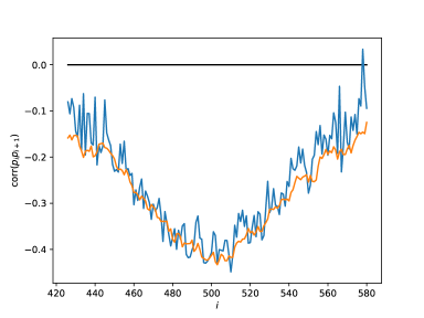
Figure 4: Correlation $\text{corr}(p_{i},p_{i+1})$. The blue curve is a numerical estimate for the ergodic average of $\text{corr}(p_{i},p_{i+1})$ after evolving the system from the same initial conditions as considered in [4] for $t=10^{8}$, a time at which the spreading law $w\propto t^{1/6}$ is already clearly visible. The orange curve shows $\text{corr}(p_{i},p_{i+1})$ in the prethermal ensemble constructed from data in a window of size $10$ around each site. Both curves have been averaged over disorder. The black line is the $T$-independent value of $\text{corr}(p_{i},p_{i+1})$ in a thermal state.

The latter quantity is only approximately conserved, so that this ensemble is pre-thermal rather than properly thermal, see [42, 43] for an extensive analysis and discussion of this prethermal phase in the disorder-free Klein-Gordon chain. For the sake of justifying transport equations, this prethermal phase serves just as well as the thermal phase.

Conclusion — We investigated the disordered Klein-Gordon chain with an anharmonic perturbation. A mathematical theorem shows that the decorrelation time $t_{q}$ for this chain grows faster than any polynomial in $1/\lambda$: the chain is asymptotically localized. On the other hand, numerics is consistent with the scaling $t_{q}\propto 1/\lambda^{4}$ for a broad range of values. The latter scaling corresponds to the anomalous spreading of wavepackets $w(t)\propto t^{1/6}$ observed in a series of previous works. We conclude that state-of-the-art numerics may not be capable of capturing the true long-time behaviour of the system and that the anomalous spreading law is most likely a transient behaviour, giving way at later times to a spreading law smaller than any polynomial.

a

SUPPLEMENTARY MATERIAL

I Linear fluctuating hydrodynamics

We provide some details on linear fluctuating hydrodynamics, which is used in the main text to derive the normal diffusive behaviour for the decorrelation measure $\eta(t)$. In the definition of $\eta(t)$, we replace the observables $X_{k}$ by the hydrodynamic local fields $\phi_{x}$.

I.1 Setting

We rename the field as $\phi(t)_{x}=\delta\rho_{x}(t)$. We pass to Fourier variables

$$\partial_{t}\phi_{k}(t)=-Dk^{2}\phi_{k}(t)+iak\zeta_{k}(t),$$ (5)

where $k\in[-\pi,\pi]$, and $\overline{\zeta_{k}(s)}=\zeta_{-k}(s)$. The distribution of the noise is Guassian and

$$\langle\zeta_{k}(s)\rangle=0\qquad\langle\zeta_{k}(s)\zeta_{k^{\prime}}(s^{\prime})\rangle=\delta(k+k^{\prime})\delta(s-s^{\prime}).$$

The solution of (5) is

$$\phi_{k}(t)=e^{-tk^{2}D}\phi_{k}(0)+iak\int_{0}^{t}dse^{-(t-s)k^{2}D}\zeta_{k}(s).$$

The stationary state of $\phi_{k}$ is Gaussian with mean zero and covariance

$$\langle\phi_{k}\phi_{k^{\prime}}\rangle=-a^{2}k^{2}\int_{0}^{t}dse^{-2k^{2}D(t-s)}\delta(k+k^{\prime})=\frac{a^{2}}{2D}\delta(k+k^{\prime}),$$

which allows to determine $a$, since we know that the stationary state in real space, namely

$$\langle\phi_{x}\rangle=0,\qquad\langle\phi_{x}\phi_{x^{\prime}}\rangle=C\delta({x-x^{\prime})},$$

with

$$C=\sum_{i}\left(\langle E_{0},E_{i}\rangle-\langle E_{0}\rangle\langle E_{i}\rangle\right),$$

with $\langle\cdot;\cdot\rangle$ computed in the microscopic Gibbs state. Hence, we find the form of the fluctuation-dissipation relation

$$a^{2}=2DC.$$

I.2 Computation of the decorrelation time

The decorrelation measure $\eta$ for the local fields $\phi_{x}$ is given by

$$\eta_{x}(t)=\frac{\langle(\phi_{x}(t)-\phi_{x}(0))^{2}\rangle}{2\langle\phi_{x}^{2}\rangle},$$

$$\langle(\phi_{x}(t)-\phi_{x}(0))^{2}\rangle=$$

$$\int dkdk^{\prime}e^{ix(k+k^{\prime})}\left((e^{tk^{2}D}-1)(e^{-t{k^{\prime}}^{2}D}-1)\langle\phi_{k}(0)\phi_{k^{\prime}}(0)\rangle\right.$$

$$\left.\qquad+(ak)^{2}\delta(k+k^{\prime})\int_{0}^{t}ds\,e^{-2(t-s)k^{2}D}\right)=$$

$$\int dkdk^{\prime}e^{ix(k+k^{\prime})}\left((e^{-tk^{2}D}-1)(e^{-t{k^{\prime}}^{2}D}-1)\frac{a^{2}}{2D}\delta(k+k^{\prime})\right.$$

$$\left.\qquad+(ak)^{2}\delta(k+k^{\prime})\int_{0}^{t}ds\,e^{-2(t-s)k^{2}D}\right)=$$

$$\int dk(e^{-tk^{2}D}-1)^{2}\frac{a^{2}}{2D}+\int dk(ak)^{2}\int_{0}^{t}ds\,e^{-2(t-s)k^{2}D}.$$

The $t\to\infty$ limit of this expression is $2\pi\times 2\times\frac{a^{2}}{2D}$, which equals $2\langle\phi_{x}^{2}\rangle$. We therefore get, for large $t$

$$\langle(\phi_{x}(t)-\phi_{x}(0))^{2}\rangle-2\langle\phi_{x}^{2}\rangle\approx\frac{a^{2}}{2D}\left(\frac{1}{\sqrt{2tD}}-\frac{2}{\sqrt{tD}}\right),$$

and hence

$$\frac{\langle(\phi_{x}(t)-\phi_{x}(0))^{2}\rangle}{2\langle\phi_{x}^{2}\rangle}=1-\frac{1-(2\sqrt{2})^{-1}}{\sqrt{tD}}.$$

II Details on Figure 2 and 3

The theoretical value $\eta(t)$ involves averages over the thermal ensemble and over disorder. We explain here how we compute this in practice. We approximate

$$\eta(t)\approx\frac{1}{D}\sum_{d=1}^{D}\eta^{(d)}(t),$$ (6)

with

$$\eta^{(d)}(t)=\\ \frac{1}{L}\sum_{i=1}^{L}\frac{\frac{1}{2}\left(X_{i}^{(d,d)}(0)-X_{i}^{(d,d)}(t)\right)^{2}}{\frac{1}{N}\sum_{p=1}^{N}\left(X_{i}^{(d,p)}(0)\right)^{2}-\left(\frac{1}{N}\sum_{p=1}^{N}X_{i}^{(d,p)}(0)\right)^{2}},$$ (7)

Here the subscripts $d,p$ in $X_{i}^{(d,p)}$ refer to a realization of disorder and a choise of initial conditions, respectively. We used $L=80$, $D=200$, and $N=1000$. The different initial conditions were generated as follows. First, we evolved the system according to Langevin equation with coupling strength equal $0.1$ from random initial conditions for $200$ time units using a simple leapfrog method with time step $0.05$. Taking the output of this simulation as thermal initial conditions we continued with the integration of Hamilton equations of motion measuring the decorelation level on a numerical grid $t_{j}=j\cdot 10^{s}$, $j=0,1,\dots,10^{5}$ with $s=5$ for $\gamma\leq 0.03$ and $s=3$ otherwise (we also use $s=0$ for $\lambda\geq 0.5$ for times up to $t=10^{4}$).

Decorrelation times where extracted in the following manner. We divided $200$ disorder realization into sets of $20$ realizations over which we averaged $\eta^{(d)}(t)$ obtaining $10$ estimates for $\eta(t)$. For each them we searched for the smallest time $t_{j}$ such that $\eta(t_{j})\geq\eta_{*}$, where $\eta_{*}$ is the desired level of decorrelation. With the use of a linear fit to the points $\eta(t_{j-1})$ and $\eta(t_{j})$ we extracted the time $t_{*}$ at which $\eta_{*}$ is reached. The plotted deccorelation times are means of these $t_{*}$ and error bars indicate their standard error.

III Details for Figure 4

The blue curve is a numerical estimate for the ergodic average of $\text{corr}(p_{i},p_{i+1})$. This correlation was measured after evolving the system ($W=4$, $\gamma=1$, and fixed $\omega_{L/2}=1$) from the initial condition $p_{i}=0$, $q_{i}=c\delta_{i,L/2}$ for $t=10^{8}$, with $c$ such that the total energy equals $E=0.4$. The orange curve shows $\text{corr}(p_{i},p_{i+1})$ in the prethermal ensemble constructed from data in a window of size $10$ around each site. Both curves have been averaged over disorder. The black line is the value of $\text{corr}(p_{i},p_{i+1})$ in a equilibrium state. It is zero because the equilibrium state is a product for the momentum variables.

IV Extracting the effective anharmonicity from the width $w$

We describe here how to assign an effective anharmonicity to a wavepacket of total energy $E$ and width $w$. If the wavepacket had a box form, with width $\ell$, then the local energy density (which is equal to the temperature at small anharmonicity) is $E/\ell$ and so the effective anharmonicity is obviously

$$\lambda=\gamma(E/\ell).$$

Furthermore, a short computation gives the relation between $w$ and $\ell$, namely $\ell=2\sqrt{3}w$, so that we finally arrive at the estimate

$$\lambda=\frac{1}{2\sqrt{3}}\gamma\frac{E}{w}.$$ (8)

Actually, assuming a box form is not a bad approximation, as one can see in [41]. It becomes exact for the nonlinear diffusion equation with $D\propto\rho^{n}$ in the limit of $n\to\infty$. The other extreme case is a Gaussian wavepacket, which appears in the opposite limit $n\to 0$. For a Gaussian packet, the energy density is not constant, so we take a weighted average to determine the temperature:

$$T=\int dx(1/E)(\rho(x))^{2},\qquad\rho(x)=\frac{E}{\sqrt{2\pi}w}e^{-\frac{1}{2}(\frac{x}{w})^{2}}.$$

This gives $E/(2\sqrt{\pi}w)$ and so we arrive at

$$\lambda=\frac{1}{2\sqrt{\pi}}\gamma\frac{E}{w}.$$ (9)

Comparing to (8), we see that the difference between both estimates is only 3 percent.

V Comparison with [14]

In [14], the spreading of a wave packet is investigated numerically for disordered nonlinear discrete-time quantum walks, and the behavior $w\propto t^{1/6}$ is observed for 12 decades in time. As eq. (6) in the SM of [14] shows, the equations of motion display a cubic non-linearity at low densities, as in the KG and the DNLS chains. All these systems belong thus to the same class, consistently with the obsevations for the spreading of the wave packet. Nevertheless, a fair and direct comparison with our numerics is strictly speaking impossible due to the differences between the models. Yet, we can estimate the value of the effective non-linearity reached in [14] when the packet has maximally spread out.

Reasoning as for the KG chain, we find that the effective non-linearity in the set-up of [14] is given by

$$\lambda^{\prime}=g\rho,$$

where $g$ is the bare non-linearity and $\rho$ the density of the packet. From the data in [14], we can estimate $\lambda^{\prime}$ in two ways. First, from Fig. 2 in [14], we estimate roughly that $\rho\approx 0.001$ at the final time $t_{f}=2\times 10^{12}$, hence $\lambda^{\prime}\approx 3\times 10^{-3}$ since $g=3$. Second, from Fig. 3 in [14], we also see that at the final time $w^{2}\approx 10^{6}$. Using the procedure described in previous section, we obtain value $\lambda^{\prime}\approx 9\times 10^{-4}$. Either way, despite having run the simulations for much longer times, it is thus not clear to us that the results in [14] outperform previous simulations if one considers the effective anharmonicity as the relevant parameter.

VI Probing smaller anharmonicities within spreading numerics

From Fig. 1. in [4] we see that $w^{2}\approx 900$ is reached at the final time $t_{0}=10^{10}$ for $E=0.05$. Using the method of Section IV, this corresponds to the value $\lambda_{0}\approx 5\times 10^{-4}$ of the effective anharmonicity. In order to reach the smallest effective anharmonicity considered in our present work, i.e. $\lambda_{1}=2\times 10^{-4}$, under the assumption that the spreading follows the law $w\propto t^{1/6}$, we estimate that the simulation would need to be continued up to time

$$t_{1}=\left(\frac{\lambda_{0}}{\lambda_{1}}\right)^{6}t_{0}.$$ (10)

Plugging in the numerical values we obtain $t_{1}\approx 2.5\times 10^{12}$, hence 250 times longer than in [4]. Of course, all estimates of this type should be taken with a grain of salt. Small changes in anharmonicity lead to huge changes in the time.

References

- [1] P. W. Anderson, “Absence of diffusion in certain random lattices,” Phys. Rev., vol. 109, pp. 1492–1505, Mar 1958.
- [2] A. S. Pikovsky and D. L. Shepelyansky, “Destruction of anderson localization by a weak nonlinearity,” Phys. Rev. Lett., vol. 100, p. 094101, Mar 2008.
- [3] I. García-Mata and D. L. Shepelyansky, “Delocalization induced by nonlinearity in systems with disorder,” Phys. Rev. E, vol. 79, p. 026205, Feb 2009.
- [4] S. Flach, D. O. Krimer, and C. Skokos, “Universal spreading of wave packets in disordered nonlinear systems,” Phys. Rev. Lett., vol. 102, p. 024101, Jan 2009.
- [5] C. Skokos, D. O. Krimer, S. Komineas, and S. Flach, “Delocalization of wave packets in disordered nonlinear chains,” Phys. Rev. E, vol. 79, p. 056211, May 2009.
- [6] C. Skokos and S. Flach, “Spreading of wave packets in disordered systems with tunable nonlinearity,” Phys. Rev. E, vol. 82, p. 016208, Jul 2010.
- [7] M. Mulansky and A. Pikovsky, “Spreading in disordered lattices with different nonlinearities,” EPL, vol. 90, p. 10015, May 2010.
- [8] T. Terao, “Localization-delocalization transition and subdiffusion of discrete nonlinear schrödinger equation in three dimensions,” Phys. Rev. E, vol. 83, p. 056611, May 2011.
- [9] M. Larcher, T. V. Laptyeva, J. D. Bodyfelt, F. Dalfovo, M. Modugno, and S. Flach, “Subdiffusion of nonlinear waves in quasiperiodic potentials,” New J. Phys., vol. 14, p. 103036, Oct 2012.
- [10] B. Min, T. Li, M. Rosenkranz, and W. Bao, “Subdiffusive spreading of a bose-einstein condensate in random potentials,” Phys. Rev. A, vol. 86, p. 053612, Nov 2012.
- [11] X. Yu and S. Flach, “Enhancement of chaotic subdiffusion in disordered ladders with synthetic gauge fields,” Phys. Rev. E, vol. 90, p. 032910, Sep 2014.
- [12] I. I. Yusipov, T. V. Laptyeva, A. Y. Pirova, I. B. Meyerov, S. Flach, and M. V. Ivanchenko, “Quantum subdiffusion with two- and three-body interactions,” Eur. Phys. J. B, vol. 90, p. 66, Apr 2017.
- [13] B. Senyange, B. M. Manda, and C. Skokos, “Characteristics of chaos evolution in one-dimensional disordered nonlinear lattices,” Phys. Rev. E, vol. 98, p. 052229, Nov 2018.
- [14] I. Vakulchyk, M. V. Fistul, and S. Flach, “Wave packet spreading with disordered nonlinear discrete-time quantum walks,” Phys. Rev. Lett., vol. 122, p. 040501, Jan 2019.
- [15] Y. Kati, X. Yu, and S. Flach, “Density resolved wave packet spreading in disordered gross-pitaevskii lattices,” SciPost Physics Core, vol. 3, p. 006, Oct 2020.
- [16] C. Skokos, E. Gerlach, and S. Flach, “Frequency map analysis of spatiotemporal chaos in the nonlinear disordered klein–gordon lattice,” Int. J. Bifurcation Chaos, vol. 32, p. 2250074, Apr 2022.
- [17] J. Fröhlich, T. Spencer, and C. E. Wayne, “Localization in disordered, nonlinear dynamical systems,” Journal of Statistical Physics, vol. 42, pp. 247–274, 1986.
- [18] G. Benettin, J. Fröhlich, and A. Giorgilli, “A nekhoroshev-type theorem for hamiltonian systems with infinitely many degrees of freedom,” Communications in Mathematical Physics, vol. 119, pp. 95–108, Mar 1988.
- [19] J. Pöschel, “Small divisors with spatial structure in infinite dimensional hamiltonian systems,” Communications in Mathematical Physics, vol. 127, no. 2, pp. 351–393, 1990.
- [20] J. Bourgain and W.-M. Wang, Chapter 2. Diffusion Bound for a Nonlinear Schrödinger Equation, pp. 21–42. Princeton: Princeton University Press, 2007.
- [21] M. Johansson, G. Kopidakis, and S. Aubry, “Kam tori in 1d random discrete nonlinear schrödinger model?,” EPL, vol. 91, p. 50001, Sep 2010.
- [22] W.-M. Wang and Z. Zhang, “Long time anderson localization for the nonlinear random schrödinger equation,” Journal of Statistical Physics, vol. 134, pp. 953–968, Mar 2009.
- [23] S. Fishman, Y. Krivolapov, and A. Soffer, “Perturbation theory for the nonlinear schrödinger equation with a random potential,” Nonlinearity, vol. 22, no. 12, p. 2861, 2009.
- [24] S. Fishman, Y. Krivolapov, and A. Soffer, “The nonlinear schrödinger equation with a random potential: results and puzzles,” Nonlinearity, vol. 25, no. 4, p. R53, 2012.
- [25] D. M. Basko, “Weak chaos in the disordered nonlinear schrödinger chain: Destruction of anderson localization by arnold diffusion,” Annals of Physics, vol. 326, pp. 1577–1655, Jul 2011.
- [26] H. Cong, Y. Shi, and Z. Zhang, “Long-time anderson localization for the nonlinear schrödinger equation revisited,” Journal of Statistical Physics, vol. 182, p. 10, Jan 2021.
- [27] W. De Roeck and F. Huveneers, “Asymptotic localization of energy in nondisordered oscillator chains,” Communications on Pure and Applied Mathematics, vol. 68, no. 9, pp. 1532–1568, 2015.
- [28] F. Huveneers, “Drastic fall-off of the thermal conductivity for disordered lattices in the limit of weak anharmonic interactions,” Nonlinearity, vol. 26, p. 837, Feb 2013.
- [29] V. Oganesyan, A. Pal, and D. A. Huse, “Energy transport in disordered classical spin chains,” Phys. Rev. B, vol. 80, p. 115104, Sep 2009.
- [30] M. Kumar, A. Kundu, M. Kulkarni, D. A. Huse, and A. Dhar, “Transport, correlations, and chaos in a classical disordered anharmonic chain,” Phys. Rev. E, vol. 102, p. 022130, Aug 2020.
- [31] W. De Roeck and F. Huveneers, “Asymptotic quantum many-body localization from thermal disorder,” Communications in Mathematical Physics, vol. 332, pp. 1017–1082, Jul 2014.
- [32] A. Bols and W. De Roeck, “Asymptotic localization in the Bose-Hubbard model,” Journal of Mathematical Physics, vol. 59, p. 021901, Feb 2018.
- [33] I. Y. Gol’dshtein, S. A. Molchanov, and L. A. Pastur, “A pure point spectrum of the stochastic one-dimensional schrödinger operator,” Functional Analysis and Its Applications, vol. 11, no. 1, pp. 1–8, 1977.
- [34] H. Kunz and B. Souillard, “Sur le spectre des opérateurs aux différences finies aléatoires,” Communications in Mathematical Physics, vol. 78, no. 2, pp. 201 – 246, 1980.
- [35] R. Carmona, “Exponential localization in one dimensional disordered systems,” Duke Mathematical Journal, vol. 49, no. 1, pp. 191 – 213, 1982.
- [36] W. De Roeck, F. Huveneers, and O. A. Prośniak, “Slow transport in a one-dimensional disordered anharmonic chain.” in prep.
- [37] N. Minami, “Local fluctuation of the spectrum of a multidimensional anderson tight binding model,” Communications in mathematical physics, vol. 177, pp. 709–725, 1996.
- [38] G. M. Graf and A. Vaghi, “A remark on the estimate of a determinant by minami,” Letters in Mathematical Physics, vol. 79, pp. 17–22, 2007.
- [39] M. Aizenman and S. Warzel, “On the joint distribution of energy levels of random schrödinger operators,” Journal of Physics A: Mathematical and Theoretical, vol. 42, no. 4, p. 045201, 2008.
- [40] F. Klopp, “Decorrelation estimates for the eigenlevels of the discrete anderson model in the localized regime,” Communications in Mathematical Physics, vol. 303, no. 1, pp. 233–260, 2011.
- [41] B. Tuck, “Some explicit solutions to the non-linear diffusion equation,” Journal of Physics D: Applied Physics, vol. 9, p. 1559, Aug 1976.
- [42] C. B. Mendl, J. Lu, and J. Lukkarinen, “Thermalization of oscillator chains with onsite anharmonicity and comparison with kinetic theory,” Phys. Rev. E, vol. 94, p. 062104, Dec 2016.
- [43] F. Huveneers and J. Lukkarinen, “Prethermalization in a classical phonon field: Slow relaxation of the number of phonons,” Phys. Rev. Res., vol. 2, p. 022034, May 2020.