Decentralized Riemannian Conjugate Gradient Method on the Stiefel Manifold

Abstract

The conjugate gradient method is a crucial first-order optimization method that generally converges faster than the steepest descent method, and its computational cost is much lower than the second-order methods. However, while various types of conjugate gradient methods have been studied in Euclidean spaces and on Riemannian manifolds, there has little study for those in distributed scenarios. This paper proposes a decentralized Riemannian conjugate gradient descent (DRCGD) method that aims at minimizing a global function over the Stiefel manifold. The optimization problem is distributed among a network of agents, where each agent is associated with a local function, and communication between agents occurs over an undirected connected graph. Since the Stiefel manifold is a non-convex set, a global function is represented as a finite sum of possibly non-convex (but smooth) local functions. The proposed method is free from expensive Riemannian geometric operations such as retractions, exponential maps, and vector transports, thereby reducing the computational complexity required by each agent. To the best of our knowledge, DRCGD is the first decentralized Riemannian conjugate gradient algorithm to achieve global convergence over the Stiefel manifold.

1 Introduction

In large-scale systems such as machine learning, control, and signal processing, data is often stored in a distributed manner across multiple nodes and it is also difficult for a single (centralized) server to meet the growing computing needs. Therefore, decentralized optimization has gained significant attention in recent years due to it can effectively address the above two potential challenges. In this paper, we consider the following distributed smooth optimization problem over the Stiefel manifold:

$$\min\frac{1}{n}\sum_{i=1}^{n}f_{i}\left(x_{i}\right),$$ (1)

$$\text{ s.t. }x_{1}=\cdots=x_{n},\quad x_{i}\in\mathcal{M},\quad\forall i=1,2,\ldots,n,$$

where $n$ is the number of agents, $f_{i}$ is the local function at each agent, and $\mathcal{M}:=\operatorname{St}(d,r)=\{x\in\mathbb{R}^{d\times r}|x^{\top}x=\emph{I}_{r}\}$ is the Stiefel manifold ($r\leq d$) (Zhu, 2017; Sato, 2022). Many important large-scale tasks can be written as the optimization problem (1), e.g., the principle component analysis (Ye and Zhang, 2021), eigenvalue estimation (Chen et al., 2021), dictionary learning (Raja and Bajwa, 2015), and deep neural networks with orthogonal constraint (Vorontsov et al., 2017; Huang et al., 2018; Eryilmaz and Dundar, 2022).

Decentralized optimization has recently attracted increasing attention in Euclidean spaces. Among the methods explored, the decentralized (sub)-gradient method stands out as a straightforward way combining local gradient descent and consensus error reduction (Nedic and Ozdaglar, 2009; Yuan et al., 2016). Further, in order to converge to a stationary point (i.e., exact convergence) with fixed step size, various algorithms have considered the local historical information, e.g., gradient tracking algorithm (Qu and Li, 2017; Yuan et al., 2018), primal-dual framework (Alghunaim et al., 2020), EXTRA (Shi et al., 2015), and ADMM (Shi et al., 2014; Aybat et al., 2017), when each local function is convex.

However, none of the above studies can solve the problem (1) since the Stiefel manifold is a non-convex set. Based on the viewpoint of Chen et al. (2021), the Stiefel manifold is an embedded sub-manifold in Euclidean space. Thus, with the help of Riemannian optimization (i.e., optimization on Riemannian manifolds) (Absil et al., 2008; Boumal et al., 2019; Sato, 2021), the problem (1) can be thought as a constrained problem in Euclidean space. The Riemannian optimization nature brings more challenges for consensus construction design. For instance, a straightforward way is to take the average $\frac{1}{n}\sum_{i=1}^{n}x_{i}$ in Euclidean space. However, the arithmetic average does not apply to the Riemannian manifold because the arithmetic average of points can be outside of the manifold. To address this problem, Riemannian consensus methods have been developed (Shah, 2017), but it needs to use an asymptotically infinite number of consensus steps for convergence. Subsequently, Wang and Liu (2022) combined the gradient tracking algorithm with an augmented Lagrangian function to achieve the single step of consensus. Recently, Chen et al. (2021) proposed a decentralized Riemannian gradient descent algorithm over the Stiefel manifold, which also requires only finite step of consensus to achieve the convergence rate of $\mathcal{O}(1/\sqrt{K})$. Simultaneously, the corresponding gradient tracking version with the convergence rate of $\mathcal{O}(1/K)$ to reach a stationary point was presented. On this basis, Deng and Hu (2023) replaced retractions with projection operators, thus establishing a decentralized projected Riemannian gradient descent algorithm over the compact submanifold to achieve the convergence rate of $\mathcal{O}(1/\sqrt{K})$. Similarly, the corresponding gradient tracking version also achieved the convergence rate of $\mathcal{O}(1/K)$.

In this paper, we address the decentralized conjugate gradient method on Riemannian manifolds, which we refer to as the decentralized Riemannian conjugate gradient descent (DRCGD) method. The conjugate gradient method is an important first-order optimization method that generally converges faster than the steepest descent method, and its computational cost is much lower than the second-order methods. Hence, the conjugate gradient methods are highly attractive for solving large-scale optimization (Sato, 2022). Recently, Riemannian conjugate gradient methods have been studied, however, expensive operations such as parallel translations, vector transports, exponential maps, and retractions are required. For instance, some studies use a theoretical approach, i.e., parallel translation along the geodesics (Smith, 1995; Edelman and Smith, 1996; Edelman et al., 1998), which hinders the practical applicability. More generally, other studies utilize a vector transport (Ring and Wirth, 2012; Sato and Iwai, 2015; Zhu, 2017; Sakai and Iiduka, 2020, 2021) or inverse retraction (Zhu and Sato, 2020) to simplify the execution of each iteration of Riemannian conjugate gradient methods. Nonetheless, there is room for computational improvement.

This paper focuses on designing an efficient Riemannian conjugate gradient algorithm to solve the problem (1) over any undirected connected graph. Our contributions are as follows:

1. We propose a decentralized Riemannian conjugate gradient method whose global convergence is established under an extended assumption. To the best of our knowledge, it is the first Riemannian conjugate gradient algorithm for distributed optimization.

2. With an intuitive concept of Riemannian conjugate gradient methods, we further develop the projection operator so that the expensive retraction and vector transport are completely replaced by it. Therefore, the proposed method is retraction-free and vector transport-free to make the algorithm computationally cheap.

3. Numerical experiments are performed to demonstrate the effectiveness of the theoretical results. The experimental results are used to compare the performances of state-of-the-art ones on eigenvalue problems.

2 Preliminaries

2.1 Notation

The undirected connected graph $G=(\mathcal{V},\mathcal{E})$, where $\mathcal{V}=\{1,2,\cdots,n\}$ is the set of agents and $\mathcal{E}$ is the set of edges. When $W$ is the adjacency matrix of $G$, we have $W_{ij}=W_{ji}$ and $W_{ij}>0$ if an edge $(i,j)\in\mathcal{E}$ and otherwise $W_{ij}=0$. We use $\mathbf{x}$ to denote the collection of all local variables $x_{i}$ by stacking them, i.e., $\mathbf{x}^{\top}:=(x_{1}^{\top},x_{2}^{\top},\cdots,x_{n}^{\top})$. Then define $f(\mathbf{x}):=\frac{1}{n}\sum_{i=1}^{n}f_{i}(x_{i})$. We denote the $n$-fold Cartesian product of $\mathcal{M}$ with itself as $\mathcal{M}^{n}=\mathcal{M}\times\cdots\times\mathcal{M}$, and use $[n]:=\{1,2,\cdots,n\}$. For any $x\in\mathcal{M}$, we denote the tangent space and normal space of $\mathcal{M}$ at $x$ as $T_{x}\mathcal{M}$ and $N_{x}\mathcal{M}$, respectively. We mark $\|\cdot\|$ as the Euclidean norm. The Euclidean gradient of $f$ is $\nabla f(x)$ and the Riemannian gradient of $f$ is $\operatorname{grad}f(x)$. Let $\emph{I}_{d}$ and $\textbf{1}_{n}\in\mathbb{R}^{n}$ be the $d\times d$ identity matrix and a vector of all entries one, respectively. Let $\mathbf{W}^{t}:=W^{t}\otimes\emph{I}_{d}$, where $t$ is a positive integer and $\otimes$ denotes the Kronecker product.

2.2 Riemannian manifold

We define the distance of a point $y\in\mathbb{R}^{d\times r}$ onto $\mathcal{M}$ by

$$\operatorname{dist}(x,\mathcal{M}):=\inf_{y\in\mathcal{M}}\|y-x\|,$$

then, for any radius $R>0$, the $R$-tube around $\mathcal{M}$ can be defined as the set:

$$U_{\mathcal{M}}(R):=\{x:\operatorname{dist}(x,\mathcal{M})\leq R\}.$$

Furthermore, we define the nearest-point projection of a point $y\in\mathbb{R}^{d\times r}$ onto $\mathcal{M}$ by

$$\mathcal{P}_{\mathcal{M}}(x):=\arg\min_{y\in\mathcal{M}}\|y-x\|.$$

Based on Definition 3, we can say a closed set $\mathcal{M}$ is $R$-proximally smooth if the projection $\mathcal{P}_{\mathcal{M}}(x)$ is a singleton whenever $\operatorname{dist}(x,\mathcal{M})<R$. In particular, when $\mathcal{M}$ is the Stiefel manifold, it is a 1-proximally smooth set (Balashov and Kamalov, 2021). And these properties will be crucial for us to demonstrate the convergence.

Definition 2.1.

Clarke et al. (1995) An $R$-proximally smooth set $\mathcal{M}$ satisfies that
(i) for any real $\gamma\in(0,R)$, the estimate holds:

$$\left\|\mathcal{P}_{\mathcal{M}}(x)-\mathcal{P}_{\mathcal{M}}(y)\right\|\leq\frac{R}{R-\gamma}\|x-y\|,\quad\forall x,y\in U_{\mathcal{M}}(\gamma).$$ (2)

(ii) for any point $x\in\mathcal{M}$ and a normal $v\in N_{x}\mathcal{M}$, the following inequality holds for all $y\in\mathcal{M}$:

$$\langle v,y-x\rangle\leq\frac{\|v\|}{2R}\|y-x\|^{2}.$$ (3)

To proceed the optimization on Riemannian manifolds, we introduce a key concept called the retraction operator in Definition 2.2. Obviously, the exponential maps (Absil et al., 2008) also satisfies this definition, so that the retraction operator is not unique.

Definition 2.2.

Absil et al. (2008) A smooth map $\mathcal{R}:T\mathcal{M}\rightarrow\mathcal{M}$ is called a retraction on a smooth manifold $\mathcal{M}$ if the retraction of $\mathcal{R}$ to the tangent space $T_{x}\mathcal{M}$ at any point $x\in\mathcal{M}$, denoted by $\mathcal{R}_{x}$, satisfies the following conditions:
(i) $\mathcal{R}$ is continuously differentiable.
(ii) $\mathcal{R}_{x}(0_{x})=x$, where $0_{x}$ is the zero element of $T_{x}\mathcal{M}$.
(iii) $\mathrm{D}\mathcal{R}_{x}(0_{x})=\operatorname{id}_{T_{x}\mathcal{M}}$, the identity mapping on $T_{x}\mathcal{M}$.

Furthermore, we can introduce a well-known concept called a vector transport, which as a special case of parallel translation can be explicitly formulated on the Stiefel manifold. Compared to parallel translation, a vector transport is easier and cheaper to compute (Sato, 2021). Using the Whitney sum $T\mathcal{M}\oplus T\mathcal{M}:=\{(\eta,\xi)|\eta,\xi\in T_{x}\mathcal{M},x\in\mathcal{M}\}$, we can define a vector transport as follows.

Definition 2.3.

Absil et al. (2008) A map $\mathscr{T}:T\mathcal{M}\oplus T\mathcal{M}\rightarrow T\mathcal{M}:(\eta,\xi)\mapsto\mathscr{T}_{\eta}(\xi)$ is called a vector transport on $\mathcal{M}$ if there exists a retraction $\mathcal{R}$ on $\mathcal{M}$ and $\mathscr{T}$ satisfies the following conditions for any $x\in\mathcal{M}$:
(i) $\mathscr{T}_{\eta}(\xi)\in T_{\mathcal{R}_{x}(\eta)}\mathcal{M},\quad\eta,\xi\in T_{x}\mathcal{M}$.
(ii) $\mathscr{T}_{x_{x}}(\xi)=\xi,\quad\xi\in T_{x}\mathcal{M}$.
(iii) $\mathscr{T}_{\eta}(a\xi+b\zeta)=a\mathscr{T}_{\eta}(\xi)+b\mathscr{T}_{\eta}(\zeta),\quad a,b\in\mathbb{R},\quad\eta,\xi,\zeta\in T_{x}\mathcal{M}$ .

Example 2.4.

Absil et al. (2008) On a Riemannian manifold $\mathcal{M}$ with a retraction $\mathcal{R}$, we can construct a vector transport $\mathscr{T}^{R}:T\mathcal{M}\oplus T\mathcal{M}\rightarrow T\mathcal{M}:(\eta,\xi)\mapsto\mathscr{T}_{\eta}^{R}(\xi)$ defined by

$$\mathscr{T}_{\eta}^{R}(\xi):=\mathrm{D}\mathcal{R}_{x}(\eta)[\xi],\quad\eta,\xi\in T_{x}\mathcal{M},\quad x\in\mathcal{M},$$

called the differentiated retraction.

3 Consensus problem on Stiefel manifold

Let $x_{1},\cdots,x_{n}\in\mathcal{M}$ be the local variables of each agent, we denote the Euclidean average point of $x_{1},\cdots,x_{n}$ by

$$\hat{x}:=\frac{1}{n}\sum_{i=1}^{n}x_{i}.$$ (4)

In Euclidean space, one can use $\sum_{i=1}^{n}\|x_{i}-\hat{x}\|^{2}$ to measure the consensus error. Instead, on the Stiefel manifold $\operatorname{St}(d,r)$, we use the induced arithmetic mean (Sarlette and Sepulchre, 2009), defined as follows:

$$\bar{x}:=\arg\min_{y\in\operatorname{St}(d,r)}\sum_{i=1}^{n}\|y-x_{i}\|^{2}=\mathcal{P}_{\operatorname{St}}(\hat{x}),$$ (5)

where $\mathcal{P}_{\operatorname{St}}(\cdot)$ is the orthogonal projection onto $\operatorname{St}(d,r)$. Considering the Riemannian optimization, the Riemannian gradient of $f_{i}(x)$ on $\operatorname{St}(d,r)$, endowed with the induced Riemannian metric from the Euclidean inner product $\langle\cdot,\cdot\rangle$, is given by

$$\operatorname{grad}f_{i}(x)=\mathcal{P}_{T_{x}\mathcal{M}}(\nabla f_{i}(x)),$$ (6)

where $\mathcal{P}_{T_{x}\mathcal{M}}(\cdot)$ is the orthogonal projection onto $T_{x}\mathcal{M}$. More specifically (Edelman et al., 1998; Absil et al., 2008), for any $y\in\mathbb{R}^{d\times r}$, we have

$$\mathcal{P}_{T_{x}\mathcal{M}}(y)=y-\frac{1}{2}x(x^{\top}y+y^{\top}x).$$ (7)

Subsequently, the $\epsilon$-stationary point of problem (1) is given by Definition 3.1.

Definition 3.1.

Chen et al. (2021) The set of points $\mathbf{x}^{\top}=(x_{1}^{\top}x_{2}^{\top}\cdots x_{n}^{\top})$ is called an $\epsilon$-stationary point of problem (1) if the following holds:

$$\frac{1}{n}\sum_{i=1}^{n}\left\|x_{i}-\bar{x}\right\|^{2}\leq\epsilon\quad\text{ and }\quad\|\operatorname{grad}f(\bar{x})\|^{2}\leq\epsilon,$$ (8)

where $f(\bar{x})=\frac{1}{n}\sum_{i=1}^{n}f_{i}(\bar{x})$.

To achieve the stationary point given in Definition 3.1, the consensus problem over $\operatorname{St}(d,r)$ needs to be considered to minimize the following quadratic loss function

$$\min\varphi^{t}(\mathbf{x}):=\frac{1}{4}\sum_{i=1}^{n}\sum_{j=1}^{n}W_{ij}^{t}\left\|x_{i}-x_{j}\right\|^{2},$$ (9)

$$\text{ s.t. }x_{i}\in\mathcal{M},\forall i\in[n]\text{, }$$

where the positive integer $t$ is used to indicate the $t$-th power of the doubly stochastic matrix $W$. Note that $W_{ij}^{t}$ is computed through performing $t$ steps of communication on the tangent space, and satisfies the following assumption.

Assumption 1

We assume that the undirected graph $G$ is connected and $W$ is doubly stochastic, i.e., (i) $W=W^{\top}$; (ii) $W_{ij}\geq 0$ and $0<W_{ii}<1$ for all $i,j$; (iii) Eigenvalues of $W$ lie in $(-1,1]$. The second largest singular value $\sigma_{2}$ of $W$ lies in $\sigma_{2}\in[0,1)$.

Throughout the paper, we assume that the local function $f_{i}(x)$ is Lipschitz smooth, which is a standard assumption in theoretical analysis of the optimization problem (Jorge and Stephen, 2006; Zeng and Yin, 2018; Deng and Hu, 2023).

Assumption 2

Each local function $f_{i}(x)$ has $L$-Lipschitz continuous gradient

$$\|\nabla f_{i}(x)-\nabla f_{i}(y)\|\leq L\|x-y\|,\quad i\in[n],$$ (10)

and let $L_{f}:=\max_{x\in\operatorname{St}(d,r)}\|\nabla f_{i}(x)\|$. Therefore, $\nabla f(x)$ is also $L$-Lipschitz continuous in the Euclidean space and $L_{f}\geq\max_{x\in\operatorname{St}(d,r)}\|\nabla f(x)\|$.

With the properties of projection operators, we can derive the similar Lipschitz inequality on the Stiefel manifold as the Euclidean-type one (Nesterov, 2013) in the following lemma.

Lemma 3.2.

(Lipschitz-type inequality) Under Assumption 2, for any $x,y\in\operatorname{St}(d,r)$, if $f(x)$ is $L$-Lipschitz smooth in the Euclidean space, then there exists a constant $L_{g}=L+2L_{f}$ such that

$$\|\operatorname{grad}f_{i}(x)-\operatorname{grad}f_{i}(y)\|\leq L_{g}\|x-y\|,\quad i\in[n].$$ (11)

Proof 3.3.

The proofs can be found in Appendix A.

Furthermore, since the Stiefel manifold is a 1-proximally smooth set (Balashov and Kamalov, 2021), the projection operator on $\operatorname{St}(d,r)$ has the following properties based on Definition 3

$$\left\|\mathcal{P}_{\mathcal{M}}(x)-\mathcal{P}_{\mathcal{M}}(y)\right\|\leq\frac{1}{1-\gamma}\|x-y\|,\quad\forall x,y\in U_{\mathcal{M}}(\gamma),\gamma\in(0,1),$$ (12)

$$\langle v,y-x\rangle\leq\frac{\|v\|}{2}\|y-x\|^{2}.$$ (13)

These two inequalities will be used to characterize the local convergence of the consensus problem.

4 Decentralized Riemannian conjugate gradient method

In this section, we will present a decentralized Riemannian conjugate gradient descent (DRCGD) method for solving the problem (1) described in Algorithm 1 and yield the convergence analysis.

4.1 The algorithm

We now introduce conjugate gradient methods on a Riemannian manifold $\mathcal{M}$. Our goal is to develop the decentralized version of Riemannian conjugate gradient methods on $\operatorname{St}(d,r)$. The generalized Riemannian conjugate gradient descent (Absil et al., 2008; Sato, 2021) iterates as

$$x_{k+1}=\mathcal{R}_{x_{k}}(\alpha_{k}\eta_{k}),$$ (14)

where $\eta_{k}$ is the search direction on the tangent space $T_{x_{k}}\mathcal{M}$ and $\alpha_{k}>0$ is the step size. Then an operation called retraction $\mathcal{R}_{x_{k}}$ is performed to ensure feasibility, whose definition is given in Definition 2.2. It follows from Definition 2.3 that we have $\mathscr{T}_{\alpha_{k}\eta_{k}}(\eta_{k})\in T_{x_{k+1}}\mathcal{M}$. Thus, the search direction (Sato, 2021) can be iterated as

$$\eta_{k+1}=-\operatorname{grad}f(x_{k+1})+\beta_{k+1}\mathscr{T}_{\alpha_{k}\eta_{k}}(\eta_{k}),\quad k=0,1,\cdots,$$ (15)

where the scalar $\beta_{k+1}\in\mathbb{R}$. Since $\operatorname{grad}f(x_{k+1})\in T_{x_{k+1}}\mathcal{M}$ and $\beta_{k+1}\eta_{k}\in T_{x_{k}}\mathcal{M}$, they belong to different tangent spaces and cannot be added. Hence, the vector transport in Definition 2.3 needs to be used to map a tangent vector in $T_{x_{k}}\mathcal{M}$ to one in $T_{x_{k+1}}\mathcal{M}$.

However, vector transports are still computationally expensive, which significantly affects the efficiency of our algorithm. To extend search directions in the decentralized scenario together with computationally cheap needs, we perform the following update of decentralized search directions:

$$\eta_{i,k+1}=-\operatorname{grad}f_{i}(x_{i,k+1})+\beta_{i,k+1}\mathcal{P}_{T_{x_{i,k+1}}\mathcal{M}}\left(\sum_{j=1}^{n}W_{ij}^{t}\eta_{j,k}\right),\quad i\in[n],$$ (16)

where $\operatorname{grad}f_{i}(x_{i,k+1})\in T_{x_{i,k+1}}\mathcal{M}$ and $\eta_{i,k}\in T_{x_{i,k}}\mathcal{M}$. Note that $\sum_{j=1}^{n}W_{ij}^{t}\eta_{j,k}$ is clearly not on the tangent space $T_{x_{i,k+1}}\mathcal{M}$ and even not on the tangent space $T_{x_{i,k}}\mathcal{M}$. Therefore, it is important to define the projection of $\sum_{j=1}^{n}W_{ij}^{t}\eta_{j,k}$ to $T_{x_{i,k+1}}\mathcal{M}$ so that we can compute the addition in the same tangent space $T_{x_{i,k+1}}\mathcal{M}$ to update the $\eta_{i,k+1}$. On the other hand, similar to the decentralized projected Riemannian gradient descent (Deng and Hu, 2023), the DRCGD performs the following update in the $k$-th iteration

$$x_{i,k+1}=\mathcal{P}_{\mathcal{M}}\left(\sum_{j=1}^{n}W_{ij}^{t}x_{j,k}+\alpha_{k}\eta_{i,k}\right),\quad i\in[n].$$ (17)

The Riemanian gradient step with a unit step size, i.e., $\mathcal{P}_{\mathcal{M}}\left(\sum_{j=1}^{n}W_{ij}^{t}x_{j,k}\right)$, is utilized in the above iteration for the consensus problem (9). So far, we have presented the efficient method by replacing both retractions and vector transports with projection operators.

Regarding $\beta_{k+1}$, there are six standard types in the Euclidean space, which were proposed by Fletcher and Reeves (1964), Dai and Yuan (1999), Fletcher (2000), Polak and Ribiere (1969) and Polyak (1969), Hestenes et al. (1952), and Liu and Storey (1991), respectively. Furthermore, the Riemannian version of $\beta_{k+1}$ was given in (Sato, 2022). Ring and Wirth (2012) analyzed the Riemannian conjugate gradient with a specific scalar $\beta_{k+1}^{\mathrm{R}-\mathrm{FR}}$, which is a natural generalization of $\beta_{k+1}^{\mathrm{FR}}$ in (Fletcher and Reeves, 1964). In this paper, we yield a naive extension of $\beta_{k+1}^{\mathrm{R}-\mathrm{FR}}$ in terms of the decentralized type

$$\beta_{i,k+1}^{\mathrm{R}-\mathrm{FR}}=\frac{\left\langle\operatorname{grad}f_{i}(x_{i,k+1}),\operatorname{grad}f_{i}(x_{i,k+1})\right\rangle_{x_{i,k+1}}}{\left\langle\operatorname{grad}f_{i}(x_{i,k}),\operatorname{grad}f_{i}(x_{i,k})\right\rangle_{x_{i,k}}}=\frac{\left\|\operatorname{grad}f_{i}(x_{i,k+1})\right\|_{x_{i,k+1}}^{2}}{\left\|\operatorname{grad}f_{i}(x_{i,k})\right\|_{x_{i,k}}^{2}},$$ (18)

where the “$\mathrm{R}-$” stands for “Riemannian” and “$\mathrm{FR}$” stands for “Fletcher-Reeves” type (Fletcher and Reeves, 1964). With the above preparations, we present the DRCGD method described in Algorithm 1. The step 3 first performs a consensus step and then update the local variable using search directions $\eta_{i,k}$. The step 4 uses the decentralized version of $\beta_{k+1}^{\mathrm{R}-\mathrm{FR}}$. The step 5 is to project the search direction onto the tangent space $T_{x_{i,k+1}}\mathcal{M}$, which follows a projection update.

Algorithm 1 Decentralized Riemannian Conjugate Gradient Descent (DRCGD) for solving Eq.(1).

0:  Initial point $\mathbf{x}_{0}\in\mathcal{M}^{n}$, an integer $t$, set $\eta_{i,0}=-\operatorname{grad}f_{i}(x_{i,0})$. {for each node $i\in[n]$, in parallel}

1:  for $k=0,\cdots$ do

2:     Choose diminishing step size $\alpha_{k}=\mathcal{O}(1/\sqrt{k})$

3:     Update $x_{i,k+1}=\mathcal{P}_{\mathcal{M}}\left(\sum_{j=1}^{n}W_{ij}^{t}x_{j,k}+\alpha_{k}\eta_{i,k}\right)$

4:     Compute $\beta_{i,k+1}=\|\operatorname{grad}f_{i}(x_{i,k+1})\|^{2}/\|\operatorname{grad}f_{i}(x_{i,k})\|^{2}$

5:     Update $\eta_{i,k+1}=-\operatorname{grad}f_{i}(x_{i,k+1})+\beta_{i,k+1}\mathcal{P}_{T_{x_{i,k+1}}\mathcal{M}}\left(\sum_{j=1}^{n}W_{ij}^{t}\eta_{j,k}\right)$

6:  end for

To analyze the convergence of the proposed algorithm, the following assumptions on the step size $\alpha_{k}$ are also needed (Sato, 2022).

Assumption 3

The step size $\alpha_{k}>0$ satisfies the following conditions:
(i) $\alpha_{k}$ is decreasing

$$\lim_{k\rightarrow\infty}\alpha_{k}=0,\quad\lim_{k\rightarrow\infty}\frac{\alpha_{k+1}}{\alpha_{k}}=1.$$ (19)

(ii) For constant $c_{1}$ and $c_{2}$ with $0<c_{1}<c_{2}<1$, the Armijo condition on $\mathcal{M}$ is

$$f_{i}(x_{i,k+1})\leq f_{i}(x_{i,k})+c_{1}\alpha_{k}\langle\operatorname{grad}f_{i}(x_{i,k}),\eta_{i,k}\rangle_{x_{i,k}}.$$ (20)

(iii) The strong Wolfe condition is

$$\left|\left\langle\operatorname{grad}f_{i}\left(x_{i,k+1}\right),\mathscr{T}_{\alpha_{k}\eta_{i,k}}^{R}(\eta_{i,k})\right\rangle_{x_{i,k+1}}\right|\leq c_{2}\left|\left\langle\operatorname{grad}f_{i}\left(x_{i,k}\right),\eta_{i,k}\right\rangle_{x_{i,k}}\right|.$$ (21)

4.2 Convergence analysis

This subsection focuses on the global convergence analysis of our DRCGD algorithm, where Theorem 4.3, Theorem 4.7, and Theorem 4.13 are very crucial, which give the locally linear convergence of consensus error, the convergence of each agent, and the global convergence, respectively.

Let us first present the linear convergence of consensus error. For the iteration scheme $x_{i,k+1}=\mathcal{P}_{\mathcal{M}}\left(\sum_{j=1}^{n}W_{ij}^{t}x_{j,k}+\alpha_{k}\eta_{i,k}\right)$ where $\alpha_{k}>0$ and $\eta_{i,k}\in T_{x_{i,k}}\mathcal{M}$, the following lemma yields that, for $\mathbf{x}_{k}$ in the neighborhood $\mathcal{N}$, the iterates $\mathbf{x}_{k+1}$ also remain in this neighborhood $\mathcal{N}$.

Lemma 4.1.

Let $x_{i,k+1}=\mathcal{P}_{\mathcal{M}}\left(\sum_{j=1}^{n}W_{ij}^{t}x_{j,k}+\alpha_{k}\eta_{i,k}\right)$. On the basis of Assumption 1, if $\mathbf{x}_{k}\in\mathcal{N}:=\{\mathbf{x}:\|\hat{x}-\bar{x}\|\leq\gamma/2\}$, $\|\eta_{i,k}\|\leq C$, $0<\alpha_{k}\leq\frac{\gamma(1-\gamma)}{4C}$, and $t\geq\left\lceil\log_{\sigma_{2}}\left(\frac{\gamma(1-\gamma)}{4\sqrt{n}\zeta}\right)\right\rceil$ with $\zeta:=\max_{x,y\in\mathcal{M}}\|x-y\|$, then

$$\sum_{j=1}^{n}W_{ij}^{t}x_{j,k}+\alpha_{k}\eta_{i,k}\in U_{\mathcal{M}}(\gamma),\quad i=1,\cdots,n,$$ (22)

$$\|\hat{x}_{k+1}-\bar{x}_{k+1}\|\leq\frac{1}{2}\gamma.$$ (23)

Proof 4.2.

The proofs can be found in Appendix B.1.

In Lemma 23, the search direction $\eta_{i,k}$ is required to be bounded. Let $\eta_{i,k}=0$, then we can consider the convergence of consensus error.

Theorem 4.3.

(Linear convergence of consensus error). Let $x_{i,k+1}=\mathcal{P}_{\mathcal{M}}\left(\sum_{j=1}^{n}W_{ij}^{t}x_{j,k}\right)$. On the basis of Assumption 1, if $t\geq\max\left\{\left\lceil\log_{\sigma_{2}}(1-\gamma)\right\rceil,\left\lceil\log_{\sigma_{2}}\left(\frac{\gamma(1-\gamma)}{4\sqrt{n}\zeta}\right)\right\rceil\right\}$ and $\mathbf{x}_{k}\in\mathcal{N}:=\{\mathbf{x}:\|\hat{x}-\bar{x}\|\leq\gamma/2\}$, then the following linear convergence with rate $\sigma_{2}^{t}/(1-\gamma)<1$ holds

$$\|\mathbf{x}_{k+1}-\bar{\mathbf{x}}_{k+1}\|\leq\frac{\sigma_{2}^{t}}{1-\gamma}\|\mathbf{x}_{k}-\bar{\mathbf{x}}_{k}\|$$

Proof 4.4.

The proofs can be found in Appendix B.2.

On the Stiefel manifold, by utilizing the 1-proximally smooth property of projection operators, we establish the locally linear convergence of consensus error with a rate of $\sigma_{2}^{t}/(1-\gamma)$, where $t$ can be any positive integer, which is consistent with the cases in the Euclidean space (Nedic et al., 2010; Nedić et al., 2018).

Different from the assumption of the bounded of a vector transport in (Sato, 2022), we give an extended assumption about the projection operator in the decentralized scenario. Specifically, we assume, for each $k\geq 0$, that the following inequality holds

$$\left|\left\langle g_{i,k+1},\mathcal{P}_{T_{x_{i,k+1}}\mathcal{M}}\left(\sum_{j=1}^{n}W_{ij}^{t}\eta_{j,k}\right)\right\rangle_{x_{i,k+1}}\right|\leq\left|\left\langle g_{i,k+1},\mathscr{T}_{\alpha_{k}\eta_{i,k}}^{R}\left(\eta_{i,k}\right)\right\rangle_{x_{i,k+1}}\right|,$$ (24)

which will be used as a substitute to proceed the following demonstration. Next, we consider proving the convergence of the Fletcher-Reeves-type DRCGD method for each agent, i.e., we use $\beta_{i,k+1}^{\mathrm{R}-\mathrm{FR}}$ in Eq.(18). See Al-Baali (1985) for its Euclidean version and Sato (2022) for its Riemannian version.

Lemma 4.5.

In Alogrithm 1 with $\beta_{i,k+1}=\beta_{i,k+1}^{\mathrm{R}-\mathrm{FR}}$ in Eq. (18) and Eq. (24), assume that $\alpha_{k}$ satisfies the strong Wolfe conditions in Eq.(20) and Eq.(21) with $0<c_{1}<c_{2}<1/2$, for each $k\geq 0$. If $\operatorname{grad}f_{i}(x_{i,k})\neq 0$ for each $k\geq 0$, then $\eta_{i,k}$ as a descent direction satisfies

$$-\frac{1}{1-c_{2}}\leq\frac{\left\langle\operatorname{grad}f_{i}(x_{i,k}),\eta_{i,k}\right\rangle_{x_{i,k}}}{\left\|\operatorname{grad}f_{i}(x_{i,k})\right\|_{x_{i,k}}^{2}}\leq-\frac{1-2c_{2}}{1-c_{2}}.$$ (25)

Proof 4.6.

The proofs can be found in Appendix C.1.

Subsequently, we proceed to the convergence property of each agent. The proof below is based on the Riemannian version given in Sato (2022).

Theorem 4.7.

In Alogrithm 1 with $\beta_{i,k+1}=\beta_{i,k+1}^{\mathrm{R}-\mathrm{FR}}$ in Eq. (18) and Eq. (24), assume that $\alpha_{k}$ satisfies the strong Wolfe conditions in Eq.(20) and Eq.(21) with $0<c_{1}<c_{2}<1/2$, for each $k\geq 0$. If $f_{i}$ is bounded below and is of class $C^{1}$, and the Riemannian version (Ring and Wirth, 2012; Sato and Iwai, 2015) of Zoutendijk’s Theorem (Nocedal and Wright, 1999) holds, then we yield

$$\lim_{k\rightarrow\infty}\inf\|\operatorname{grad}f_{i}(x_{i,k})\|_{x_{i,k}}=0,\quad i=1,\cdots,n.$$ (26)

Proof 4.8.

The proofs can be found in Appendix C.2.

At last, we can establish the global convergence of our DRCGD method based on Theorem 4.3 and Theorem 4.7. We now investigate the uniform boundedness of $\|\bm{\eta}_{k}\|$ in the following lemma.

Lemma 4.9.

Let $\{\mathbf{x}_{k}\}$ be the sequence generated by Algorithm 1. Suppose that Assumptions 1 and 2 hold. If $t\geq\max\left\{\left\lceil\log_{\sigma_{2}}\left(\frac{1-\gamma}{2\sqrt{n}\zeta}\right)\right\rceil,\left\lceil\log_{\sigma_{2}}\left(\frac{1}{8\sqrt{n}C}\right)\right\rceil,\left\lceil\log_{\sigma_{2}}\left(\frac{\gamma(1-\gamma)}{4\sqrt{n}\zeta}\right)\right\rceil\right\}$, $\mathbf{x}_{0}\in\mathcal{N}$, $\|\beta_{i,k}\|\leq C$, and $0<\alpha_{k}<\min\left\{\frac{1-\gamma}{8L_{g}},\frac{\gamma(1-\gamma)}{4C}\right\}$, it follows that for all $k$, $\mathbf{x}_{k}\in\mathcal{N}$ and

$$\|\eta_{i,k}\|\leq 2L_{g},\quad\forall i\in[n].$$ (27)

Proof 4.10.

The proofs can be found in Appendix D.1.

With the above lemma, we can elaborate the relationship between the consensus error and step size.

Lemma 4.11.

Let $\{\mathbf{x}_{k}\}$ be the sequence generated by Algorithm 1. Suppose that Assumptions 1 and 2 hold. If $\mathbf{x}_{0}\in\mathcal{N}$, $\|\eta_{i,k}\|\leq 2L_{g}$, $t\geq\left\lceil\log_{\sigma_{2}}(1-\gamma)\right\rceil$, and $0<\alpha_{k}\leq\frac{\gamma(1-\gamma)}{8L_{g}}$, it follows that for all $k$, $\mathbf{x}_{k}\in\mathcal{N}$ and

$$\frac{1}{n}\|\bar{\mathbf{x}}_{k}-\mathbf{x}_{k}\|^{2}\leq C\frac{1}{(1-\gamma)^{2}}L_{g}^{2}\alpha_{k}^{2}.$$ (28)

Proof 4.12.

The proofs can be found in Appendix D.2.

With the above preparations, we will give the global convergence of the DRCGD method.

Theorem 4.13.

(Global convergence). Let $\{\mathbf{x}_{k}\}$ be the sequence generated by Algorithm 1. Suppose that Assumptions 1 and 2 hold. If $\mathbf{x}_{0}\in\mathcal{N}$ and $\|\beta_{i,k}\|\leq C$, then

$$\lim_{k\rightarrow\infty}\inf\|\operatorname{grad}f(\bar{x}_{k})\|^{2}=0.$$ (29)

Proof 4.14.

The proofs can be found in Appendix D.3.

5 Numerical experiment

In this section, we compare our proposed DRCGD method (Algorithm 1) with DRDGD method (Chen et al., 2021) and DPRGD method (Deng and Hu, 2023) on the following decentralized eigenvector problem:

$$\min_{\mathbf{x}\in\mathcal{M}^{n}}-\frac{1}{2n}\sum_{i=1}^{n}\operatorname{tr}\left(x_{i}^{\top}A_{i}^{\top}A_{i}x_{i}\right),\quad\text{ s.t. }\quad x_{1}=\ldots=x_{n},$$ (30)

where $\mathcal{M}^{n}:=\underbrace{\operatorname{St}(d,r)\times\cdots\times\operatorname{St}(d,r)}_{n}$, $A_{i}\in\mathbb{R}^{m_{i}\times d}$, $i\in[n]$ is the local data matrix for agent $i$ and $m_{i}$ is the sample size. Note that $A^{\top}:=[A_{1}^{\top},A_{2}^{\top},\cdots,A_{n}^{\top}]$ is the global data matrix. For any solution $x^{*}$ of Eq.(30), $x^{*}Q$ with an orthogonal matrix $Q\in\mathbb{R}^{r\times r}$ is also a solution. Then the distance between two points $x$ and $x^{*}$ can be defined as

$$d_{s}(x,x^{*})=\min_{Q^{\top}Q=QQ^{\top}=\emph{I}_{r}}\|xQ-x^{*}\|.$$

We employ fixed step sizes for all comparisons, i.e., the step size is set to $\alpha_{k}=\frac{\hat{\alpha}}{\sqrt{K}}$ with $K$ being the maximal number of iterations. We examine various graph matrices used to represent the topology across agents, i.e., the Erdos-Renyi (ER) network with probability $p$ and the Ring network. It follows from (Chen et al., 2021) that $W$ is the Metroplis constant matrix (Shi et al., 2015).

We measure algorithms by four metrics, i.e., the consensus error $\|\mathbf{x}_{k}-\mathbf{\bar{x}}_{k}\|$, the gradient norm $\|\mathrm{grad}f({\bar{x}}_{k})\|$, the objective function $f({\bar{x}}_{k})-f^{*}$, and the distance to the global optimum $d_{s}({\bar{x}}_{k},x^{*})$, respectively. The experiments are evaluated with the Intel(R) Core(TM) i7-12700 CPU. And the codes are implemented in Python with mpi4py.

5.1 Synthetic data

We fix $m_{1}=m_{2}=\cdots=m_{n}=1000$, $d=10$, and $r=5$. Then we generate $m_{1}\times n$ independent and identically distributed samples to obtain $A$ by following standard multi-variate Gaussian distribution. Specifically, let $A=U\Sigma V^{\top}$ be the truncated SVD where $U\in\mathbb{R}^{1000n\times d}$ and $V\in\mathbb{R}^{d\times d}$ are orthogonal matrices, and $\Sigma\in\mathbb{R}^{d\times d}$ is a diagonal matrix, then we set the singular values of $A$ to be $\Sigma_{i,i}=\Sigma_{0,0}\times\Delta^{i/2}$ where $i\in[d]$ and eigengap $\Delta\in(0,1)$. We set the maxumum iteration epoch to 200 and early stop it if $d_{s}(\bar{x}_{k},x^{*})\leq 10^{-5}$.

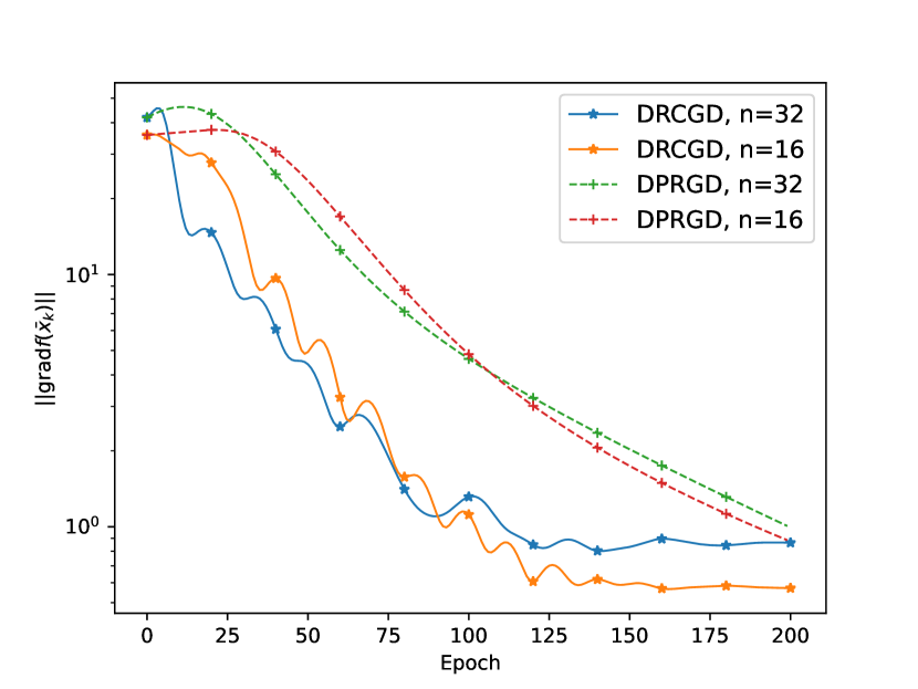
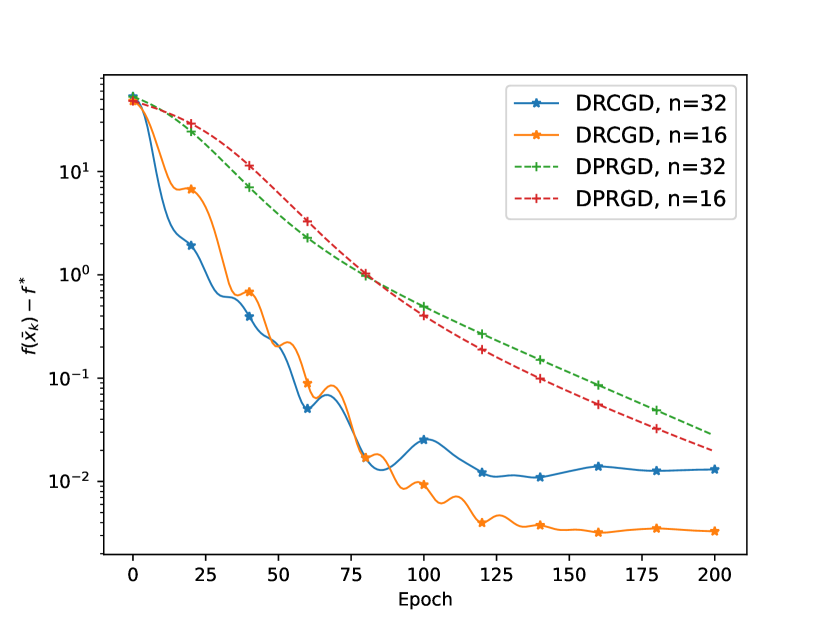
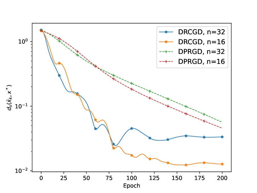
Figure 1: Numerical results on synthetic data with different numbers of agents, eigengap $\Delta=0.8$, Graph: Ring, $t=1$, $\hat{\alpha}=0.01$. y-axis: log-scale.

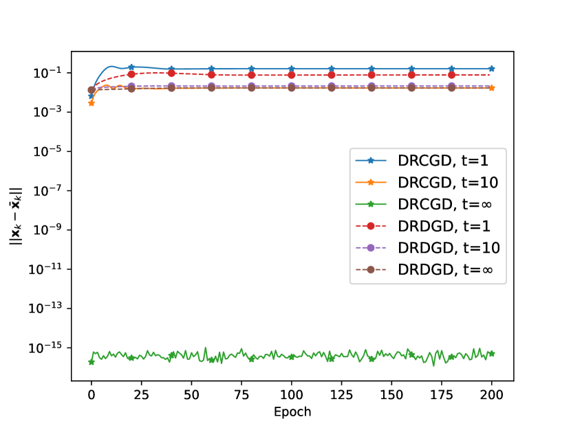
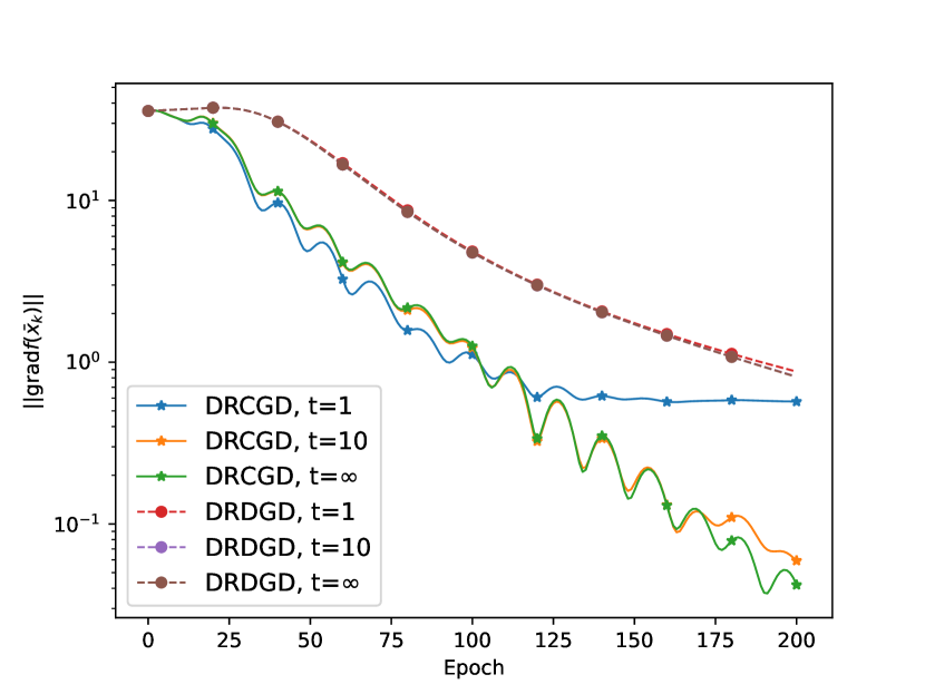
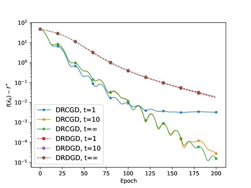
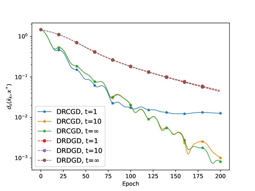
Figure 2: Numerical results on synthetic data with different numbers of consensus steps, eigengap $\Delta=0.8$, Graph: Ring, $n=16$, $\hat{\alpha}=0.01$. y-axis: log-scale.

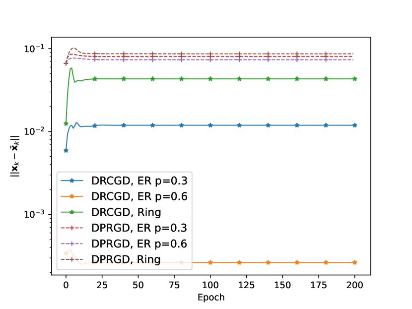
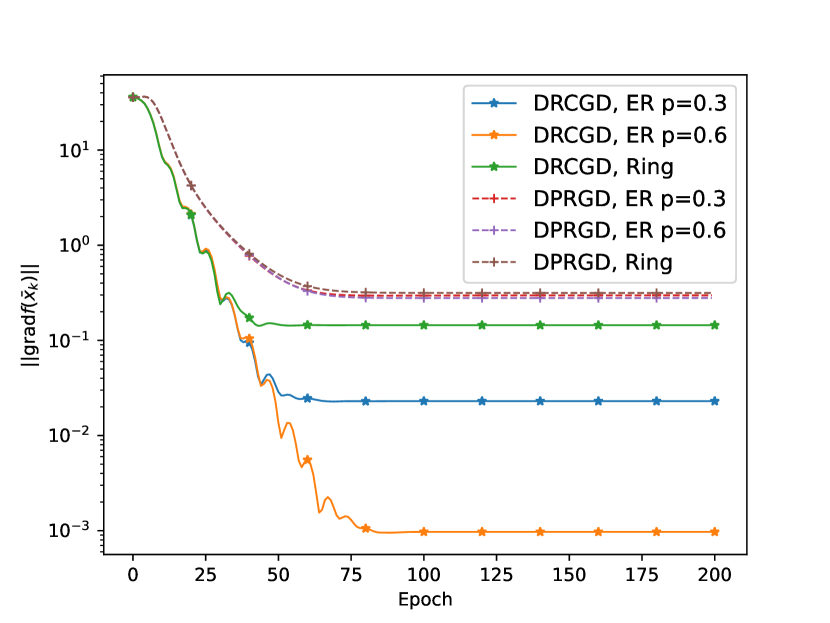
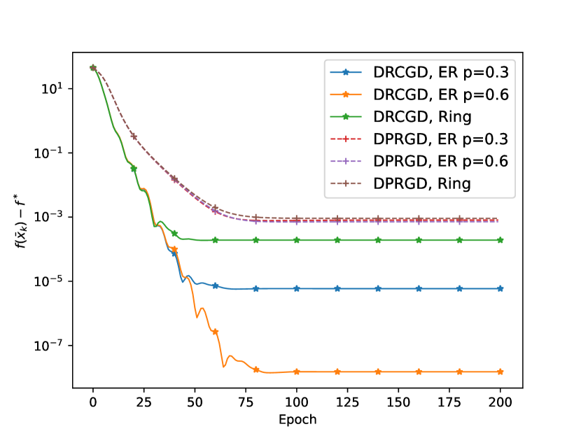
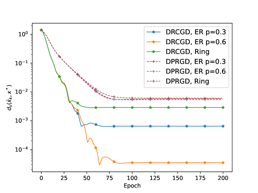
Figure 3: Numerical results on synthetic data with different network graphs, eigengap $\Delta=0.8$, $t=10$, $n=16$, $\hat{\alpha}=0.05$. y-axis: log-scale.

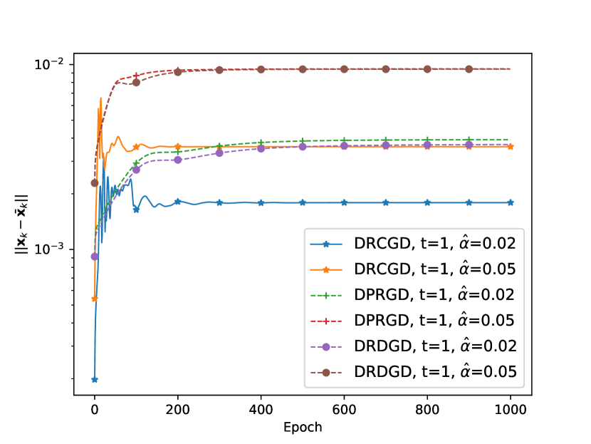
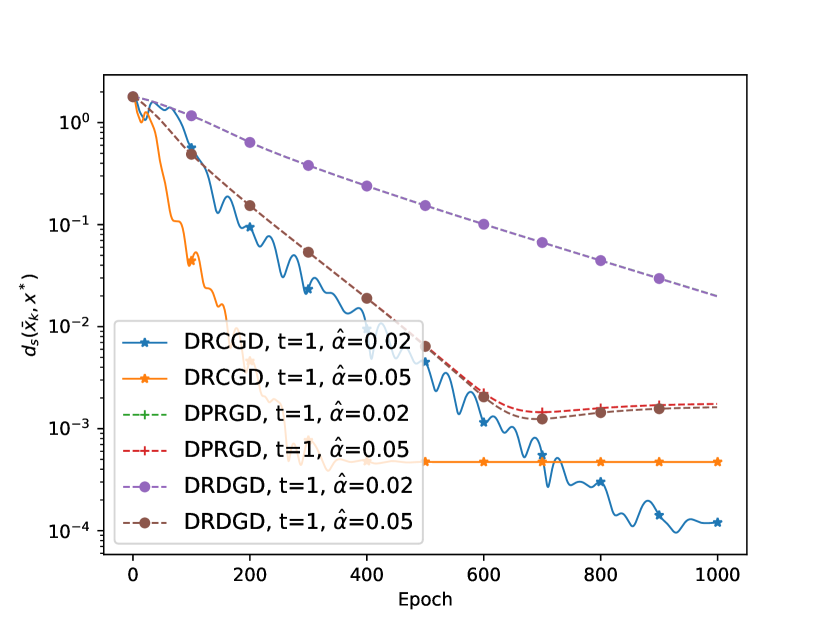
Figure 4: Numerical results on MNIST data with single-step consensus, Graph: Ring, $n=20$.

The comparison results are shown in Figures 1, 2, and 3. It can be seen from Figure 1 that our DRCGD converges faster than DPRGD under different numbers of agents ($n=16$ and $n=32$). When $n$ becomes larger, these two algorithms both converge slower. In Figure 2, DRDGD gives very similar performance under different numbers of consensus steps, i.e., $t\in\{1,10,\infty\}$, which means that the numbers of consensus steps do not affect the performance of DRDGD much. A similar phenomenon can be observed in DPRGD. In contrast, as the communication rounds $t$ increase, our DRCGD consistently achieves better performance. Note that one can achieve the case of $t\rightarrow\infty$ through a complete graph with the equally weighted matrix. For Figure 3, we see DPRGD has very close trajectories under different graphs on the four metrics. In fact, this also occurs for DRDGD. However, the connected graph ER helps our DRCGD obtain a better final solution than the connected graph Ring because ER network with the probability of each edge is a better graph connection than Ring network. Moreover, our DRCGD with ER $p=0.6$ performs better than that with ER $p=0.3$. In conclusion, DRCGD always converges faster and performs better than both DRDGD and DPRGD with different network graphs.

5.2 Real-world data

We also present some numerical results on the MNIST dataset (LeCun, 1998). For MNIST, the samples consist of 60000 hand-written images where the dimension of each image is given by $d=784$. And these samples make up the data matrix of $60000\times 784$, which is randomly and evenly partitioned into $n$ agents. We normalize the data matrix by dividing 255. Then each agent holds a local data matrix $A_{i}$ of $\frac{60000}{n}\times 784$. For brevity, we fix $t=1$, $r=5$, and $d=784$. $W$ is the Metroplis constant matrix and the graph is the Ring network. The step size of our DRCGD, DRDGD, and DPRGD is $\alpha_{k}=\frac{\hat{\alpha}}{60000}$. We set the maximum iteration epoch to 1000 and early stop it if $d_{s}(\bar{x}_{k},x^{*})\leq 10^{-5}$.

The results for MNIST data with $n=20$ are shown in Figure 4. We see that the performance of DRDGD and DPRGD are almost the same. When $\hat{\alpha}$ becomes larger, all algorithms converge faster. And our DRCGD converges much faster than both DRDGD and DPRGD.

6 Conclusion

We proposed the decentralized Riemannian conjugate gradient method for solving decentralized optimization over the Stiefel manifold. In particular, it is the first decentralized version of the Riemannian conjugate gradient. By replacing retractions and vector transports with projection operators, the global convergence was established under an extended assumption (24) on the basis of (Sato, 2021), thereby reducing the computational complexity required by each agent. Numerical results demonstrated the effectiveness of our proposed algorithm. In the future, we will further extend our algorithm to a compact sub-manifold. On the other hand, it will be interesting to develop the decentralized version of online optimization over Riemannian manifolds.

Appendix A Proofs for Lemma 3.2

Proof A.1.

Since $\operatorname{grad}f_{i}(x)=\mathcal{P}_{T_{x}\mathcal{M}}(\nabla f_{i}(x))$, we have

$$\left\|\operatorname{grad}f_{i}(x)-\operatorname{grad}f_{i}(y)\right\|=\left\|\mathcal{P}_{T_{x}\mathcal{M}}\left(\nabla f_{i}(x)\right)-\mathcal{P}_{T_{y}\mathcal{M}}\left(\nabla f_{i}(y)\right)\right\|$$ (31)

$$= \left\|\mathcal{P}_{T_{x}\mathcal{M}}\left(\nabla f_{i}(x)\right)-\mathcal{P}_{T_{x}\mathcal{M}}\left(\nabla f_{i}(y)\right)+\mathcal{P}_{T_{x}\mathcal{M}}\left(\nabla f_{i}(y)\right)-\mathcal{P}_{T_{y}\mathcal{M}}\left(\nabla f_{i}(y)\right)\right\|$$

$$\leq \left\|\mathcal{P}_{T_{x}\mathcal{M}}\left(\nabla f_{i}(x)-\nabla f_{i}(y)\right)\right\|+\left\|\mathcal{P}_{T_{x}\mathcal{M}}\left(\nabla f_{i}(y)\right)-\mathcal{P}_{T_{y}\mathcal{M}}\left(\nabla f_{i}(y)\right)\right\|$$

$$\leq \left\|\nabla f_{i}(x)-\nabla f_{i}(y)\right\|+\left\|\mathcal{P}_{T_{x}\mathcal{M}}\left(\nabla f_{i}(y)\right)-\mathcal{P}_{T_{y}\mathcal{M}}\left(\nabla f_{i}(y)\right)\right\|$$

$$\leq \left\|\nabla f_{i}(x)-\nabla f_{i}(y)\right\|+2L_{f}\|x-y\|$$

$$\leq (L+2L_{f})\|x-y\|,$$

where, by Eq.(7), the third inequality uses

$$\left\|\mathcal{P}_{T_{x}\mathcal{M}}\left(\nabla f_{i}(y)\right)-\mathcal{P}_{T_{y}\mathcal{M}}\left(\nabla f_{i}(y)\right)\right\|$$ (32)

$$= \frac{1}{2}\left\|x\left(x^{\top}\nabla f_{i}(y)+\nabla f_{i}(y)^{\top}x\right)-y\left(y^{\top}\nabla f_{i}(y)+\nabla f_{i}(y)^{\top}y\right)\right\|$$

$$\leq \frac{1}{2}\left\|x\left((x-y)^{\top}\nabla f_{i}(y)+\nabla f_{i}(y)^{\top}(x-y)\right)\right\|+\left\|(x-y)\left(y^{\top}\nabla f_{i}(y)+\nabla f_{i}(y)^{\top}y\right)\right\|$$

$$\leq \frac{1}{2}\left(\|x\|\cdot\|x-y\|\cdot\|\nabla f_{i}(y)\|+\|\nabla f_{i}(y)\|\cdot\|x-y\|+2\|x-y\|\cdot\|\nabla f_{i}(y)\|\cdot\|y\|\right)$$

$$\leq 2\|x-y\|\cdot\|\nabla f_{i}(y)\|\leq 2\max_{y\in\operatorname{St}(d,r)}\|\nabla f_{i}(y)\|\cdot\|x-y\|=2L_{f}\|x-y\|.$$

The proof is completed.

Appendix B Linear convergence of consensus error

B.1 Proofs for Lemma 23

Proof B.1.

Since $\mathbf{x}_{k}\in\mathcal{N}$, we have

$$\quad\left\|\hat{x}_{k+1}-\bar{x}_{k+1}\right\|\leq\left\|\hat{x}_{k+1}-\bar{x}_{k}\right\|\leq\frac{1}{n}\sum_{i=1}^{n}\left\|x_{i,k+1}-\bar{x}_{k}\right\|$$

$$=\frac{1}{n}\sum_{i=1}^{n}\left\|\mathcal{P}_{\mathcal{M}}\left(\sum_{j=1}^{n}W_{ij}^{t}x_{j,k}+\alpha_{k}\eta_{i,k}\right)-\mathcal{P}_{\mathcal{M}}\left(\hat{x}_{k}\right)\right\|$$

$$\leq\frac{1}{1-\gamma}\left\|\sum_{j=1}^{n}W_{ij}^{t}x_{j,k}+\alpha_{k}\eta_{i,k}-\hat{x}_{k}\right\|\leq\frac{1}{2}\gamma,$$

where the third inequality uses Eq.(12) and the fourth inequality yields

$$\left\|\sum_{j=1}^{n}W_{ij}^{t}x_{j,k}+\alpha_{k}\eta_{i,k}-\hat{x}_{k}\right\|\leq\left\|\sum_{j=1}^{n}W_{ij}^{t}x_{j,k}-\hat{x}_{k}\right\|+\|\alpha_{k}\eta_{i,k}\|$$

$$\leq\left\|\sum_{j=1}^{n}\left(W_{ij}^{t}-\frac{1}{n}\right)\left(x_{j,k}-\hat{x}_{k}\right)\right\|+\alpha_{k}C$$

$$\leq\sum_{j=1}^{n}\left|W_{ij}^{t}-\frac{1}{n}\right|\left\|x_{j,k}-\hat{x}_{k}\right\|+\alpha_{k}C$$

$$\leq\zeta\max_{i}\sum_{j=1}^{n}\left|W_{ij}^{t}-\frac{1}{n}\right|+\alpha_{k}C\leq\sqrt{n}\sigma_{2}^{t}\zeta+\alpha_{k}C\leq\frac{\gamma(1-\gamma)}{2},$$

where the fourth inequality uses that $\|x_{j,k}-\hat{x}_{k}\|\leq\frac{1}{n}\sum_{i=1}^{n}\|x_{j,k}-x_{i,k}\|\leq\zeta$ (Deng and Hu, 2023) and the fifth inequality follows from the bound on the total variation distance between any row of $W^{t}$ and $\frac{1}{n}\textbf{1}_{n}$ (Diaconis and Stroock, 1991; Boyd et al., 2004). For any $i\in[n]$, since $\bar{x}_{k}\in\mathcal{M}$ and $\gamma\in(0,1)$, we have

$$\left\|\sum_{j=1}^{n}W_{ij}^{t}x_{j,k}+\alpha_{k}\eta_{i,k}-\bar{x}_{k}\right\|\leq\left\|\sum_{j=1}^{n}W_{ij}^{t}x_{j,k}+\alpha_{k}\eta_{i,k}-\hat{x}_{k}\right\|+\left\|\hat{x}_{k}-\bar{x}_{k}\right\|$$

$$\leq\frac{\gamma(1-\gamma)}{2}+\frac{1}{2}\gamma<\gamma.$$

The proof is completed.

B.2 Proofs for Theorem 4.3

Proof B.2.

According to Lemma 23, $\|\hat{x}_{0}-\bar{x}_{0}\|\leq\frac{1}{2}\gamma$ and $\mathbf{x}_{k}\in\mathcal{N}$ for all $k\geq 0$ holds, then it holds that

$$\sum_{j=1}^{n}W_{ij}^{t}x_{j,k}\in U_{\mathcal{M}}(\gamma),\quad i=1,\cdots,n.$$

Let $\mathcal{P}_{\mathcal{M}^{n}}(\mathbf{x})^{\top}=[\mathcal{P}_{\mathcal{M}}(x_{1})^{\top},\cdots,\mathcal{P}_{\mathcal{M}}(x_{n})^{\top}]$, then with the iteration scheme $x_{i,k+1}=\mathcal{P}_{\mathcal{M}}\left(\sum_{j=1}^{n}W_{ij}^{t}x_{j,k}\right)$ we have

$$\left\|\mathbf{x}_{k+1}-\bar{\mathbf{x}}_{k+1}\right\| \leq\left\|\mathbf{x}_{k+1}-\bar{\mathbf{x}}_{k}\right\|=\left\|\mathcal{P}_{\mathcal{M}^{n}}\left(\mathbf{W}^{t}\mathbf{x}_{k}\right)-\mathcal{P}_{\mathcal{M}^{n}}\left(\hat{\mathbf{x}}_{k}\right)\right\|$$ (33)

$$\leq\frac{1}{1-\gamma}\left\|\mathbf{W}^{t}\mathbf{x}_{k}-\hat{\mathbf{x}}_{k}\right\|=\frac{1}{1-\gamma}\left\|\left(W^{t}\otimes I_{d}\right)\mathbf{x}_{k}-\hat{\mathbf{x}}_{k}\right\|$$

$$=\frac{1}{1-\gamma}\left\|\left(\left(W^{t}-\frac{1}{n}\textbf{1}_{n}\textbf{1}_{n}^{\top}\right)\otimes I_{d}\right)\left(\mathbf{x}_{k}-\hat{\mathbf{x}}_{k}\right)\right\|$$

$$\leq\frac{1}{1-\gamma}\sigma_{2}^{t}\left\|\mathbf{x}_{k}-\hat{\mathbf{x}}_{k}\right\|\leq\frac{1}{1-\gamma}\sigma_{2}^{t}\left\|\mathbf{x}_{k}-\bar{\mathbf{x}}_{k}\right\|,$$

where the second inequality uses Eq.(12). The proof is completed.

Appendix C Convergence of each agent

C.1 Proofs for Lemma 25

Proof C.1.

For ease of notation, we denote $g_{i,k}:=\operatorname{grad}f_{i}(x_{i,k})$. When $k=0$, $\eta_{i,0}=-g_{i,0}$ is the initial condition and we have

$$\frac{\left\langle g_{i,0},\eta_{i,0}\right\rangle_{x_{i,0}}}{\left\|g_{i,0}\right\|_{x_{i,0}}^{2}}=\frac{\left\langle g_{i,0},-g_{i,0}\right\rangle_{x_{i,0}}}{\left\|g_{i,0}\right\|_{x_{i,0}}^{2}}=-1.$$

Hence, Eq. (25) holds. Supposing that $\eta_{i,k}$ is a descent direction satisfying Eq. (25) for some $k$, we will prove that $\eta_{i,k+1}$ is also a descent and satisfies Eq. (25) in which $k$ is replaced with $k+1$. Based on Eq.(16) and Eq.(18), we yield

$$\frac{\left\langle g_{i,k+1},\eta_{i,k+1}\right\rangle_{x_{i,k+1}}}{\left\|g_{i,k+1}\right\|_{x_{i,k+1}}^{2}} =\frac{\left\langle g_{i,k+1},-g_{i,k+1}+\beta_{i,k+1}\mathcal{P}_{T_{x_{i,k+1}}\mathcal{M}}\left(\sum_{j=1}^{n}W_{ij}^{t}\eta_{j,k}\right)\right\rangle_{x_{i,k+1}}}{\left\|g_{i,k+1}\right\|_{x_{i,k+1}}^{2}}$$ (34)

$$=-1+\frac{\left\langle g_{i,k+1},\mathcal{P}_{T_{x_{i,k+1}}\mathcal{M}}\left(\sum_{j=1}^{n}W_{ij}^{t}\eta_{j,k}\right)\right\rangle_{x_{i,k+1}}}{\left\|g_{i,k}\right\|_{x_{i,k}}^{2}}.$$

Similar to (Sato, 2022), the assumption in Eq.(24) and the strong Wolfe condition in Eq.(21) yield

$$\left|\left\langle g_{i,k+1},\mathcal{P}_{T_{x_{i,k+1}}\mathcal{M}}\left(\sum_{j=1}^{n}W_{ij}^{t}\eta_{j,k}\right)\right\rangle_{x_{i,k+1}}\right|\leq c_{2}\left|\left\langle g_{i,k},\eta_{i,k}\right\rangle_{x_{i,k}}\right|=-c_{2}\left\langle g_{i,k},\eta_{i,k}\right\rangle_{x_{i,k}}.$$ (35)

It follows from Eq.(34) and Eq.(35) that

$$-1+c_{2}\frac{\left\langle g_{i,k},\eta_{i,k}\right\rangle_{x_{i,k}}}{\left\|g_{i,k}\right\|_{x_{i,k}}^{2}}\leq\frac{\left\langle g_{i,k+1},\eta_{k+1}\right\rangle_{x_{i,k+1}}}{\left\|g_{i,k+1}\right\|_{x_{i,k+1}}^{2}}\leq-1-c_{2}\frac{\left\langle g_{i,k},\eta_{i,k}\right\rangle_{x_{i,k}}}{\left\|g_{i,k}\right\|_{x_{i,k}}^{2}}.$$

From the induction hypothesis in Eq.(25), i.e., $\langle g_{i,k},\eta_{i,k}\rangle_{x_{i,k}}/\|g_{i,k}\|^{2}_{x_{i,k}}\geq-(1-c_{2})^{-1}$, and the assumption $c_{2}>0$, we finally obtain the following inequality

$$-\frac{1}{1-c_{2}}\leq\frac{\left\langle g_{i,k+1},\eta_{i,k+1}\right\rangle_{x_{i,k+1}}}{\left\|g_{i,k+1}\right\|_{x_{i,k+1}}^{2}}\leq-\frac{1-2c_{2}}{1-c_{2}},$$

which also implies $\langle g_{i,k+1},\eta_{i,k+1}\rangle_{x_{i,k+1}}<0$. The proof is completed.

C.2 Proofs for Theorem 4.7

Proof C.2.

We denote $g_{i,k}:=\operatorname{grad}f_{i}(x_{i,k})$ again. If $g_{i,k_{0}}=0$ holds for some $k_{0}$, then we have $\beta_{i,k_{0}}=0$ and $\eta_{i,k_{0}}=0$ from Eq.(18) and Eq.(16), which implies $x_{i,k_{0}+1}=\mathcal{P}_{\mathcal{M}}\left(\sum_{j=1}^{n}W_{ij}^{t}x_{j,k_{0}}\right)$. Based on Theorem 4.3, the consensus error converges such that $x_{i,k_{0}+1}\rightarrow x_{i,k_{0}}$ holds. Thus, we obtain $g_{i,k}=0$ for all $k\geq k_{0}$ so that Eq.(26) holds.

We next consider the case in which $g_{i,k}\neq 0$ for all $k\geq 0$. Let $\theta_{i,k}$ be the angle between $-g_{i,k}$ and $\eta_{i,k}$, i.e.,

$$\cos\theta_{i,k}=\frac{\left\langle-g_{i,k},\eta_{i,k}\right\rangle_{x_{i,k}}}{\left\|-g_{i,k}\right\|_{x_{i,k}}\left\|\eta_{i,k}\right\|_{x_{i,k}}}=-\frac{\left\langle g_{i,k},\eta_{i,k}\right\rangle_{x_{i,k}}}{\left\|g_{i,k}\right\|_{x_{i,k}}\left\|\eta_{i,k}\right\|_{x_{i,k}}}.$$ (36)

It follows from Eq.(36) and Eq.(25) that

$$\cos\theta_{i,k}\geq\frac{1-2c_{2}}{1-c_{2}}\frac{\left\|g_{i,k}\right\|_{x_{i,k}}}{\left\|\eta_{i,k}\right\|_{x_{i,k}}}.$$ (37)

Since the search directions are descent directions from Lemma 25, Zoutendijk’s Theorem together with Eq.(37) yields

$$\sum_{k=0}^{\infty}\frac{\left\|g_{i,k}\right\|^{4}_{x_{i,k}}}{\left\|\eta_{i,k}\right\|^{2}_{x_{i,k}}}<\infty.$$ (38)

Combined Eq.(25) and Eq.(35), we have

$$\left|\left\langle g_{i,k},\mathcal{P}_{T_{x_{i,k}}\mathcal{M}}\left(\sum_{j=1}^{n}W_{ij}^{t}\eta_{j,k-1}\right)\right\rangle_{x_{i,k}}\right|\leq-c_{2}\left\langle g_{i,k-1},\eta_{i,k-1}\right\rangle_{x_{i,k-1}}\leq\frac{c_{2}}{1-c_{2}}\left\|g_{i,k-1}\right\|_{x_{i,k-1}}^{2}.$$ (39)

Using Eq.(18), Eq.(24), and Eq.(39), we obtain the recurrence inequality for $\left\|\eta_{i,k}\right\|_{x_{i,k}}^{2}$:

$$\left\|\eta_{i,k}\right\|_{x_{i,k}}^{2}$$ (40)

$$=\left\|-g_{i,k}+\beta_{i,k}\mathcal{P}_{T_{x_{i,k}}\mathcal{M}}\left(\sum_{j=1}^{n}W_{ij}^{t}\eta_{j,k-1}\right)\right\|_{x_{i,k}}^{2}$$

$$\leq\left\|g_{i,k}\right\|_{x_{i,k}}^{2}+2\beta_{i,k}\left|\left\langle g_{i,k},\mathcal{P}_{T_{x_{i,k}}\mathcal{M}}\left(\sum_{j=1}^{n}W_{ij}^{t}\eta_{j,k-1}\right)\right\rangle_{x_{i,k}}\right|+\beta_{i,k}^{2}\left\|\mathcal{P}_{T_{x_{i,k}}\mathcal{M}}\left(\sum_{j=1}^{n}W_{ij}^{t}\eta_{j,k-1}\right)\right\|_{x_{i,k}}^{2}$$

$$\leq\left\|g_{i,k}\right\|_{x_{i,k}}^{2}+\frac{2c_{2}}{1-c_{2}}\beta_{i,k}\left\|g_{i,k-1}\right\|_{x_{k-1}}^{2}+\beta_{i,k}^{2}\left\|\eta_{i,k-1}\right\|_{x_{k-1}}^{2}$$

$$=\left\|g_{i,k}\right\|_{x_{i,k}}^{2}+\frac{2c_{2}}{1-c_{2}}\left\|g_{i,k}\right\|_{x_{i,k}}^{2}+\beta_{i,k}^{2}\left\|\eta_{i,k-1}\right\|_{x_{k-1}}^{2}$$

$$=c\left\|g_{i,k}\right\|_{x_{i,k}}^{2}+\beta_{i,k}^{2}\left\|\eta_{i,k-1}\right\|_{x_{k-1}}^{2},$$

where $c:=(1+c_{2})/(1-c_{2})>1$. We can successively use Eq.(40) with Eq.(18) as

$$\left\|\eta_{i,k}\right\|_{x_{i,k}}^{2}$$ (41)

$$\leq c\left(\left\|g_{i,k}\right\|_{x_{i,k}}^{2}+\beta_{i,k}^{2}\left\|g_{i,k-1}\right\|_{x_{i,k-1}}^{2}+\cdots+\beta_{i,k}^{2}\beta_{i,k-1}^{2}\cdots\beta_{i,2}^{2}\left\|g_{i,1}\right\|_{x_{i,1}}^{2}\right)+\beta_{i,k}^{2}\beta_{i,k-1}^{2}\cdots\beta_{i,1}^{2}\left\|\eta_{i,0}\right\|_{x_{i,0}}^{2}$$

$$= c\left\|g_{i,k}\right\|_{x_{i,k}}^{4}\left(\left\|g_{i,k}\right\|_{x_{i,k}}^{-2}+\left\|g_{i,k-1}\right\|_{x_{i,k-1}}^{-2}+\cdots+\left\|g_{i,1}\right\|_{x_{i,1}}^{-2}\right)+\left\|g_{i,k}\right\|_{x_{i,k}}^{4}\left\|g_{i,0}\right\|_{x_{i,0}}^{-2}$$

$$< c\left\|g_{i,k}\right\|_{x_{i,k}}^{4}\sum_{j=0}^{k}\left\|g_{i,j}\right\|_{x_{i,j}}^{-2}.$$

We can prove Eq.(26) by contradiction. We first assume that Eq.(26) does not hold. Then there exists a constant $C>0$ such that $\|g_{i,k}\|_{x_{i,k}}\geq C>0$ for all $k\geq 0$ because we also assume $g_{i,k}\neq 0$ for all $k\geq 0$ at the same time. Consequently, we have $\sum_{j=0}^{k}\|g_{i,j}\|^{2}_{x_{i,j}}\leq C^{-2}(k+1)$. Hence, based on Eq.(41), the left hand side of Eq.(38) is evaluated as

$$\sum_{k=0}^{\infty}\frac{\left\|g_{i,k}\right\|^{4}_{x_{i,k}}}{\left\|\eta_{i,k}\right\|^{2}_{x_{i,k}}}\geq\sum_{k=0}^{\infty}\frac{\epsilon^{2}}{c}\frac{1}{k+1}=\infty,$$

which contradicts Eq.(38). The proof is completed.

Appendix D Global Convergence

D.1 Proofs for Lemma 27

Proof D.1.

We prove it by induction on both $\|\eta_{i,k}\|$ and $\|\hat{x}_{k}-\bar{x}_{k}\|$. Based on Assumption 2, we have $\|\operatorname{grad}f_{i}\left(x_{i,k}\right)\|\leq\|\nabla f_{i}\left(x_{i,k}\right)\|\leq L_{f}\leq L_{g}$ due to $L_{g}=L+2L_{f}\geq L_{f}$. Then we have $\|\eta_{i,0}\|=\|\operatorname{grad}f_{i}\left(x_{i,0}\right)\|\leq L_{g}$ for all $i\in[n]$ and $\|\hat{x}_{0}-\bar{x}_{0}\|\leq\frac{1}{2}\gamma$. Suppose for some $k\geq 0$ that $\|\eta_{i,k}\|\leq 2L_{g}$ and $\|\hat{x}_{k}-\bar{x}_{k}\|\leq\frac{1}{2}\gamma$. Since $\|\eta_{i,k}\|\leq 2L_{g}$ and $\alpha_{k}<\frac{\gamma(1-\gamma)}{4C}$, it follows from Lemma 23 that

$$\sum_{j=1}^{n}W_{ij}^{t}x_{j,k}+\alpha_{k}\eta_{i,k}\in U_{\mathcal{M}}(\gamma),\quad i=1,\cdots,n,\quad\|\hat{x}_{k+1}-\bar{x}_{k+1}\|\leq\frac{1}{2}\gamma.$$

Then, we have

$$\left\|\eta_{i,k+1}+\operatorname{grad}f_{i}\left(x_{i,k}\right)\right\|$$ (42)

$$=\left\|\beta_{i,k+1}\mathcal{P}_{T_{x_{i,k+1}}\mathcal{M}}\left(\sum_{j=1}^{n}W_{ij}^{t}\eta_{j,k}\right)-\left(\operatorname{grad}f_{i}\left(x_{i,k+1}\right)-\operatorname{grad}f_{i}\left(x_{i,k}\right)\right)\right\|$$

$$\leq\beta_{i,k+1}\left\|\mathcal{P}_{T_{x_{i,k+1}}\mathcal{M}}\left(\sum_{j=1}^{n}W_{ij}^{t}\eta_{j,k}\right)\right\|+\left\|\operatorname{grad}f_{i}\left(x_{i,k+1}\right)-\operatorname{grad}f_{i}\left(x_{i,k}\right)\right\|$$

$$\leq C\left\|\sum_{j=1}^{n}\left(W_{ij}^{t}-\frac{1}{n}\right)\eta_{j,k}\right\|+L_{g}\left\|x_{i,k+1}-x_{i,k}\right\|$$

$$\leq C\sigma_{2}^{t}\sqrt{n}\max_{i}\left\|\eta_{i,k}\right\|+L_{g}\left\|x_{i,k+1}-x_{i,k}\right\|$$

$$\leq C\sigma_{2}^{t}\sqrt{n}\max_{i}\left\|\eta_{i,k}\right\|+\frac{L_{g}}{1-\gamma}\left\|\sum_{j=1}^{n}\left(W_{ij}^{t}-\frac{1}{n}\right)x_{i,k}+\alpha_{k}\eta_{i,k}\right\|$$

$$\leq\left(C\sigma_{2}^{t}\sqrt{n}+\alpha_{k}\frac{L_{g}}{1-\gamma}\right)\max_{i}\left\|\eta_{i,k}\right\|+\frac{L_{g}}{1-\gamma}\sigma_{2}^{t}\sqrt{n}\zeta$$

$$\leq\frac{1}{4}\max_{i}\left\|\eta_{i,k}\right\|+\frac{1}{2}L_{g}\leq\frac{1}{2}L_{g}+\frac{1}{2}L_{g}\leq L_{g},$$

where the second inequality uses Lemma 3.2 and the fourth inequality utilizes Eq.(12). Hence, $\|\eta_{i,k+1}\|\leq\left\|\eta_{i,k+1}+\operatorname{grad}f_{i}\left(x_{i,k}\right)\right\|+\left\|\operatorname{grad}f_{i}\left(x_{i,k}\right)\right\|\leq 2L_{g}$. The proof is completed.

D.2 Proofs for Lemma 28

Proof D.2.

Since $\|\operatorname{grad}f_{i}\left(x_{i,k}\right)\|\leq L_{g}$ and $\|\hat{x}_{0}-\bar{x}_{0}\|\leq\frac{1}{2}\gamma$, it follows from Lemma 23 that for any $k>0$, we have

$$\sum_{j=1}^{n}W_{ij}^{t}x_{j,k}+\alpha_{k}\eta_{i,k}\in U_{\mathcal{M}}(\gamma),\quad i=1,\cdots,n,$$

Let $\mathcal{P}_{\mathcal{M}^{n}}(\mathbf{x})^{\top}=[\mathcal{P}_{\mathcal{M}}(x_{1})^{\top},\cdots,\mathcal{P}_{\mathcal{M}}(x_{n})^{\top}]$. By the definition of $\bar{\mathbf{x}}_{k+1}$ and Theorem 4.3, then we yield

$$\left\|\mathbf{x}_{k+1}-\bar{\mathbf{x}}_{k+1}\right\| \leq\left\|\mathbf{x}_{k+1}-\bar{\mathbf{x}}_{k}\right\|$$ (43)

$$=\left\|\mathcal{P}_{\mathcal{M}^{n}}\left(\mathbf{W}^{t}\mathbf{x}_{k}+\alpha_{k}\bm{\eta}_{k}\right)-\mathcal{P}_{\mathcal{M}^{n}}\left(\hat{\mathbf{x}}_{k}\right)\right\|$$

$$\leq\frac{1}{1-\gamma}\left\|\mathbf{W}^{t}\mathbf{x}_{k}+\alpha_{k}\bm{\eta}_{k}-\hat{\mathbf{x}}_{k}\right\|$$

$$\leq\frac{1}{1-\gamma}\sigma_{2}^{t}\left\|\mathbf{x}_{k}-\bar{\mathbf{x}}_{k}\right\|+\frac{2}{1-\gamma}\sqrt{n}\alpha_{k}L_{g},$$

where the first inequality follows from the optimality of $\bar{\mathbf{x}}_{k+1}$, the second inequality uses Eq.(12), and the third inequality utilizes the fact that $\|\bm{\eta}_{k}\|\leq 2\sqrt{n}L_{g}$.

Let $\rho_{t}=\frac{1}{1-\gamma}\sigma_{2}^{t}$ where $0<\rho_{t}<1$, it follows from Eq.(44) that

$$\left\|\mathbf{x}_{k+1}-\bar{\mathbf{x}}_{k+1}\right\| \leq\rho_{t}\left\|\mathbf{x}_{k}-\bar{\mathbf{x}}_{k}\right\|+\frac{2}{1-\gamma}\sqrt{n}\alpha_{k}L_{g}$$ (44)

$$\leq\rho_{t}^{k+1}\left\|\mathbf{x}_{0}-\bar{\mathbf{x}}_{0}\right\|+\frac{2\sqrt{n}L_{g}}{1-\gamma}\sum_{l=0}^{k}\rho_{t}^{k-l}\alpha_{l}.$$

Let $y_{k}=\frac{\left\|\mathbf{x}_{k}-\bar{\mathbf{x}}_{k}\right\|}{\sqrt{n}\alpha_{k}}$. For a positive integer $K\leq k$, it follows from Eq.(44) that

$$y_{k+1}\leq\rho_{t}y_{k}+\frac{2}{1-\gamma}L_{g}\frac{\alpha_{k}}{\alpha_{k+1}}\leq\rho_{t}^{k+1-K}y_{K}+\frac{2}{1-\gamma}L_{g}\sum_{l=0}^{k}\rho_{t}^{k-l}\frac{\alpha_{l}}{\alpha_{l+1}}.$$

Since $\alpha_{k}=\mathcal{O}(1/L_{g})$ and $\|\bar{\mathbf{x}}_{0}-\mathbf{x}_{0}\|\leq\frac{1}{2}\sqrt{n}\gamma$, one has that $y_{0}\leq\frac{1}{2}\gamma/\alpha_{0}=\mathcal{O}(L_{g})$. Since $\lim_{k\rightarrow\infty}\frac{\alpha_{k+1}}{\alpha_{k}}=1$, there exists sufficiently large $K$ such that $\alpha_{k}/\alpha_{k+1}\leq 2,\forall k\geq K$. For $0\leq k\leq K$, there exists some $C^{\prime}>0$ such that $y_{k}^{2}\leq C^{\prime}\frac{1}{(1-\gamma)^{2}}L_{g}^{2}$, where $C^{\prime}$ is independent of $L_{g}$ and $n$. For $k\geq K$, one has that $y_{k}^{2}\leq C\frac{1}{(1-\gamma)^{2}}L_{g}^{2}$, where $C=2C^{\prime}+\frac{32}{(1-\rho_{t})^{2}}$. Hence, we get $\frac{\left\|\mathbf{x}_{k}-\bar{\mathbf{x}}_{k}\right\|^{2}}{n}\leq C\frac{1}{(1-\gamma)^{2}}L_{g}^{2}$ for all $k\geq 0$, where $C=\mathcal{O}(\frac{1}{(1-\rho_{t})^{2}})$. The proof is completed.

D.3 Proofs for Theorem 4.13

Proof D.3.

We have the following inequality:

$$\|\operatorname{grad}f(\bar{x}_{k})\|^{2}$$ (45)

$$=\left\|\frac{1}{n}\sum_{i=1}^{n}\operatorname{grad}f_{i}(x_{i,k})+\operatorname{grad}f(\bar{x}_{k})-\frac{1}{n}\sum_{i=1}^{n}\operatorname{grad}f_{i}(x_{i,k})\right\|^{2}$$

$$\leq 2\left\|\frac{1}{n}\sum_{i=1}^{n}\operatorname{grad}f_{i}(x_{i,k})\right\|^{2}+2\left\|\operatorname{grad}f(\bar{x}_{k})-\frac{1}{n}\sum_{i=1}^{n}\operatorname{grad}f_{i}(x_{i,k})\right\|^{2}$$

$$\leq 2\left\|\frac{1}{n}\sum_{i=1}^{n}\operatorname{grad}f_{i}(x_{i,k})\right\|^{2}+\frac{2}{n}\sum_{i=1}^{n}\left\|\operatorname{grad}f_{i}(\bar{x}_{k})-\operatorname{grad}f_{i}(x_{i,k})\right\|^{2}$$

$$\leq 2\left\|\frac{1}{n}\sum_{i=1}^{n}\operatorname{grad}f_{i}(x_{i,k})\right\|^{2}+\frac{2L_{g}^{2}}{n}\sum_{i=1}^{n}\left\|\bar{x}_{k}-x_{i,k}\right\|^{2}$$

$$=2\left\|\frac{1}{n}\sum_{i=1}^{n}\operatorname{grad}f_{i}(x_{i,k})\right\|^{2}+\frac{2L_{g}^{2}}{n}\left\|\bar{\mathbf{x}}_{k}-\mathbf{x}_{k}\right\|^{2},$$

where the third inequality uses Lemma 3.2. Since $\lim_{{k\rightarrow\infty}}\inf\|\operatorname{grad}f_{i}(x_{i,k})\|=0$ based on Theorem 4.3 and $\|\bar{\mathbf{x}}_{k}-\mathbf{x}_{k}\|^{2}\leq nC\frac{1}{(1-\gamma)^{2}}L_{g}^{2}\alpha_{k}^{2}$ based on Theorem 4.7, it follows from $\lim_{k\rightarrow\infty}\alpha_{k}=0$ that

$$\lim_{k\rightarrow\infty}\|\operatorname{grad}f(\bar{x}_{k})\|^{2}\leq 2\left\|\frac{1}{n}\sum_{i=1}^{n}\operatorname{grad}f_{i}(x_{i,k})\right\|^{2}+2C\frac{1}{(1-\gamma)^{2}}L_{g}^{4}\alpha_{k}^{2}=0.$$

The proof is completed.

References

- Absil et al. (2008) P-A Absil, Robert Mahony, and Rodolphe Sepulchre. Optimization algorithms on matrix manifolds. Princeton University Press, 2008.
- Al-Baali (1985) Mehiddin Al-Baali. Descent property and global convergence of the fletcher—reeves method with inexact line search. IMA Journal of Numerical Analysis, 5(1):121–124, 1985.
- Alghunaim et al. (2020) Sulaiman A Alghunaim, Ernest K Ryu, Kun Yuan, and Ali H Sayed. Decentralized proximal gradient algorithms with linear convergence rates. IEEE Transactions on Automatic Control, 66(6):2787–2794, 2020.
- Aybat et al. (2017) Necdet Serhat Aybat, Zi Wang, Tianyi Lin, and Shiqian Ma. Distributed linearized alternating direction method of multipliers for composite convex consensus optimization. IEEE Transactions on Automatic Control, 63(1):5–20, 2017.
- Balashov and Kamalov (2021) MV Balashov and RA Kamalov. The gradient projection method with armijo’s step size on manifolds. Computational Mathematics and Mathematical Physics, 61:1776–1786, 2021.
- Boumal et al. (2019) Nicolas Boumal, Pierre-Antoine Absil, and Coralia Cartis. Global rates of convergence for nonconvex optimization on manifolds. IMA Journal of Numerical Analysis, 39(1):1–33, 2019.
- Boyd et al. (2004) Stephen Boyd, Persi Diaconis, and Lin Xiao. Fastest mixing markov chain on a graph. SIAM review, 46(4):667–689, 2004.
- Chen et al. (2021) Shixiang Chen, Alfredo Garcia, Mingyi Hong, and Shahin Shahrampour. Decentralized riemannian gradient descent on the stiefel manifold. In International Conference on Machine Learning, pages 1594–1605. PMLR, 2021.
- Clarke et al. (1995) Francis H Clarke, Ronald J Stern, and Peter R Wolenski. Proximal smoothness and the lower-c2 property. J. Convex Anal, 2(1-2):117–144, 1995.
- Dai and Yuan (1999) Yu-Hong Dai and Yaxiang Yuan. A nonlinear conjugate gradient method with a strong global convergence property. SIAM Journal on optimization, 10(1):177–182, 1999.
- Deng and Hu (2023) Kangkang Deng and Jiang Hu. Decentralized projected riemannian gradient method for smooth optimization on compact submanifolds. arXiv preprint arXiv:2304.08241, 2023.
- Diaconis and Stroock (1991) Persi Diaconis and Daniel Stroock. Geometric bounds for eigenvalues of markov chains. The annals of applied probability, pages 36–61, 1991.
- Edelman and Smith (1996) Alan Edelman and Steven T Smith. On conjugate gradient-like methods for eigen-like problems. BIT Numerical Mathematics, 36(3):494–508, 1996.
- Edelman et al. (1998) Alan Edelman, Tomás A Arias, and Steven T Smith. The geometry of algorithms with orthogonality constraints. SIAM journal on Matrix Analysis and Applications, 20(2):303–353, 1998.
- Eryilmaz and Dundar (2022) Sukru Burc Eryilmaz and Aysegul Dundar. Understanding how orthogonality of parameters improves quantization of neural networks. IEEE Transactions on Neural Networks and Learning Systems, 2022.
- Fletcher and Reeves (1964) Reeves Fletcher and Colin M Reeves. Function minimization by conjugate gradients. The computer journal, 7(2):149–154, 1964.
- Fletcher (2000) Roger Fletcher. Practical methods of optimization. John Wiley & Sons, 2000.
- Hestenes et al. (1952) Magnus R Hestenes, Eduard Stiefel, et al. Methods of conjugate gradients for solving linear systems. Journal of research of the National Bureau of Standards, 49(6):409–436, 1952.
- Huang et al. (2018) Lei Huang, Xianglong Liu, Bo Lang, Adams Yu, Yongliang Wang, and Bo Li. Orthogonal weight normalization: Solution to optimization over multiple dependent stiefel manifolds in deep neural networks. In Proceedings of the AAAI Conference on Artificial Intelligence, volume 32, 2018.
- Jorge and Stephen (2006) Nocedal Jorge and J Wright Stephen. Numerical optimization. Spinger, 2006.
- LeCun (1998) Yann LeCun. The mnist database of handwritten digits. http://yann. lecun. com/exdb/mnist/, 1998.
- Liu and Storey (1991) Y Liu and C Storey. Efficient generalized conjugate gradient algorithms, part 1: theory. Journal of optimization theory and applications, 69:129–137, 1991.
- Nedic and Ozdaglar (2009) Angelia Nedic and Asuman Ozdaglar. Distributed subgradient methods for multi-agent optimization. IEEE Transactions on Automatic Control, 54(1):48–61, 2009.
- Nedic et al. (2010) Angelia Nedic, Asuman Ozdaglar, and Pablo A Parrilo. Constrained consensus and optimization in multi-agent networks. IEEE Transactions on Automatic Control, 55(4):922–938, 2010.
- Nedić et al. (2018) Angelia Nedić, Alex Olshevsky, and Michael G Rabbat. Network topology and communication-computation tradeoffs in decentralized optimization. Proceedings of the IEEE, 106(5):953–976, 2018.
- Nesterov (2013) Y Nesterov. Introductory Lectures on Convex Optimization: A Basic Course, volume 87. Springer Science & Business Media, 2013.
- Nocedal and Wright (1999) Jorge Nocedal and Stephen J Wright. Numerical optimization. Springer, 1999.
- Polak and Ribiere (1969) Elijah Polak and Gerard Ribiere. Note sur la convergence de méthodes de directions conjuguées. Revue française d’informatique et de recherche opérationnelle. Série rouge, 3(16):35–43, 1969.
- Polyak (1969) Boris Teodorovich Polyak. The conjugate gradient method in extremal problems. USSR Computational Mathematics and Mathematical Physics, 9(4):94–112, 1969.
- Qu and Li (2017) Guannan Qu and Na Li. Harnessing smoothness to accelerate distributed optimization. IEEE Transactions on Control of Network Systems, 5(3):1245–1260, 2017.
- Raja and Bajwa (2015) Haroon Raja and Waheed U Bajwa. Cloud k-svd: A collaborative dictionary learning algorithm for big, distributed data. IEEE Transactions on Signal Processing, 64(1):173–188, 2015.
- Ring and Wirth (2012) Wolfgang Ring and Benedikt Wirth. Optimization methods on riemannian manifolds and their application to shape space. SIAM Journal on Optimization, 22(2):596–627, 2012.
- Sakai and Iiduka (2020) Hiroyuki Sakai and Hideaki Iiduka. Hybrid riemannian conjugate gradient methods with global convergence properties. Computational Optimization and Applications, 77:811–830, 2020.
- Sakai and Iiduka (2021) Hiroyuki Sakai and Hideaki Iiduka. Sufficient descent riemannian conjugate gradient methods. Journal of Optimization Theory and Applications, 190(1):130–150, 2021.
- Sarlette and Sepulchre (2009) Alain Sarlette and Rodolphe Sepulchre. Consensus optimization on manifolds. SIAM journal on Control and Optimization, 48(1):56–76, 2009.
- Sato (2021) Hiroyuki Sato. Riemannian optimization and its applications, volume 670. Springer, 2021.
- Sato (2022) Hiroyuki Sato. Riemannian conjugate gradient methods: General framework and specific algorithms with convergence analyses. SIAM Journal on Optimization, 32(4):2690–2717, 2022.
- Sato and Iwai (2015) Hiroyuki Sato and Toshihiro Iwai. A new, globally convergent riemannian conjugate gradient method. Optimization, 64(4):1011–1031, 2015.
- Shah (2017) Suhail M Shah. Distributed optimization on riemannian manifolds for multi-agent networks. arXiv preprint arXiv:1711.11196, 2017.
- Shi et al. (2014) Wei Shi, Qing Ling, Kun Yuan, Gang Wu, and Wotao Yin. On the linear convergence of the admm in decentralized consensus optimization. IEEE Transactions on Signal Processing, 62(7):1750–1761, 2014.
- Shi et al. (2015) Wei Shi, Qing Ling, Gang Wu, and Wotao Yin. Extra: An exact first-order algorithm for decentralized consensus optimization. SIAM Journal on Optimization, 25(2):944–966, 2015.
- Smith (1995) Steven Smith. Optimization techniques on riemannian manifolds. Hamiltonian and Gradient Flows, Algorithms and Control, pages 113–136, 1995.
- Vorontsov et al. (2017) Eugene Vorontsov, Chiheb Trabelsi, Samuel Kadoury, and Chris Pal. On orthogonality and learning recurrent networks with long term dependencies. In International Conference on Machine Learning, pages 3570–3578. PMLR, 2017.
- Wang and Liu (2022) Lei Wang and Xin Liu. Decentralized optimization over the stiefel manifold by an approximate augmented lagrangian function. IEEE Transactions on Signal Processing, 70:3029–3041, 2022.
- Ye and Zhang (2021) Haishan Ye and Tong Zhang. Deepca: Decentralized exact pca with linear convergence rate. The Journal of Machine Learning Research, 22(1):10777–10803, 2021.
- Yuan et al. (2016) Kun Yuan, Qing Ling, and Wotao Yin. On the convergence of decentralized gradient descent. SIAM Journal on Optimization, 26(3):1835–1854, 2016.
- Yuan et al. (2018) Kun Yuan, Bicheng Ying, Xiaochuan Zhao, and Ali H Sayed. Exact diffusion for distributed optimization and learning—part i: Algorithm development. IEEE Transactions on Signal Processing, 67(3):708–723, 2018.
- Zeng and Yin (2018) Jinshan Zeng and Wotao Yin. On nonconvex decentralized gradient descent. IEEE Transactions on signal processing, 66(11):2834–2848, 2018.
- Zhu (2017) Xiaojing Zhu. A riemannian conjugate gradient method for optimization on the stiefel manifold. Computational optimization and Applications, 67:73–110, 2017.
- Zhu and Sato (2020) Xiaojing Zhu and Hiroyuki Sato. Riemannian conjugate gradient methods with inverse retraction. Computational Optimization and Applications, 77:779–810, 2020.