Frequency Compensated Diffusion Model for Real-scene Dehazing

Abstract

Due to distribution shift, deep learning based methods for image dehazing suffer from performance degradation when applied to real-world hazy images. In this paper, we consider a dehazing framework based on conditional diffusion models for improved generalization to real haze. First, we find that optimizing the training objective of diffusion models, i.e., Gaussian noise vectors, is non-trivial. The spectral bias of deep networks hinders the higher frequency modes in Gaussian vectors from being learned and hence impairs the reconstruction of image details. To tackle this issue, we design a network unit, named Frequency Compensation block (FCB), with a bank of filters that jointly emphasize the mid-to-high frequencies of an input signal. We demonstrate that diffusion models with FCB achieve significant gains in both perceptual and distortion metrics. Second, to further boost the generalization performance, we propose a novel data synthesis pipeline, HazeAug, to augment haze in terms of degree and diversity. Within the framework, a solid baseline for blind dehazing is set up where models are trained on synthetic hazy-clean pairs, and directly generalize to real data. Extensive evaluations show that the proposed dehazing diffusion model significantly outperforms state-of-the-art methods on real-world images. Our code is at https://github.com/W-Jilly/frequency-compensated-diffusion-model-pytorch.

1 Introduction

Single image dehazing aims to recover the clean image from a hazy input for improved visual quality. The hazing process is formulated by the well-known atmospheric scattering model (ASM) [39]:

$$I(p)=J(p)e^{-\beta d(p)}+A(1-e^{-\beta d(p)})$$ (1)

where $p$ is the pixel position, $I(p)$ and $J(p)$ are the hazy and haze-free image respectively. $A$ denotes the global atmospheric light. $e^{-\beta d(p)}$ is the transmission map, in which $d(p)$ is the scene depth and the scattering coefficient $\beta$ represents the degree of haze.

Existing dehazing algorithms have been impressively advanced by the emergence of deep neural networks (DNNs) [20, 12, 41, 16], but generalize poorly to real-world hazy images. An important reason is that training in a supervised manner requires hazy-clean pairs in large amounts. Due to the inaccessibility of real paired data, synthetic pairs created from ASM are widely adopted for haze simulation. Unfortunately, current ASM-based synthesis lacks ability to faithfully represent real hazy conditions. For example, $\beta$ and $A$, modeled as global constants in Eq.1, are actually found to be pixel position dependent under some conditions [62, 61], i.e., non-homogeneous ASM. Consequently, dehazing models trained on synthetic pairs work well in-distribution, but degrades dramatically when applied to real haze. To better address the problem of dehazing in real scene, many works [49, 14] are carried out within a paradigm of semi-supervised learning that assumes the availability of some real images. Domain adaptation techniques are often utilized to bridge the gap between synthetic and real data. However, the generality of DNNs is not effectively improved, as one needs to re-train the model once encountering a new scenario.

Recently, diffusion models [54, 52, 25], belonging to a family of deep generative models, emerged with impressive results that beat Generative Adversarial Network (GAN) [22] baselines on image generation. Inspired by their strong ability in modeling data distributions, there are attempts to learn the prior distribution of groundtruth images alone with diffusion models for inverse problem solving [37, 56]. In other words, the data prior is learned by unconditional diffusion models, whereas only in the generative process, an input (e.g., hazy image) ”hijacks” to guide the image generation to be consistent with the input and the prior. Despite being an universal approach, the missing of task-specific knowledge at training usually leads to an inferior performance to conditional models. To tackle this issue, conditional diffusion models are proposed to make the training of networks accept a conditioning input [48] and demonstrate remarkable performance on a variety of image-to-image applications, e.g., super-resolution [48] and deblurring [67].

Motivated by their promising results, we seek to adapt the conditional diffusion models for dehazing task. It has been reported that diffusion models, on various applications [48, 67, 46], deliver high perceptual quality outputs, but often underperform in terms of distortion measures, e.g., PSNR and SSIM, which suggests the reconstructed image details are not very well aligned. In this work, we find this to be closely related to a property of neural networks, namely spectral bias that prioritizes learning the low-frequency functions in the training [42]. However, this property is not aligned with the learning objective of diffusion models, which resembles estimating Gaussian noise vectors with uniformly distributed spectra. Their abundant high frequency modes are hence harder and slower to be learned due to the bias, which accordingly, impairs the restored high-frequency image details. To fill this gap, we propose a generic network unit, named Frequency Compensation block (FCB), to allow selective emphasis on the mid-to-high frequencies of an input signal. The block structure (see Fig.1) mimics the filter design in signal processing through which only the frequency band of interest is allowed to pass. It can be plugged into any encoder-decoder architecture to ease the learning of an unnatural Gaussian-like target. Experiments validate the effectiveness of FCB in improving both the perceptual quality and distortion measures of diffusion models.

Next, we propose a novel data augmentation pipeline, HazeAug, to improve the generalization ability of diffusion models for ”blind” dehazing. In a blind setting, the dehazing model is trained on synthetic pairs only, and directly applied to real hazy images. We hypothesize that the diffusion models possess much stronger generalization ability if trained on richer data. However, ASM-based synthesis is limited in its ability to describe diverse and complex hazy conditions. To address this limitation, HazeAug aims to augment haze in terms of degree and diversity. Specifically, HazeAug generates more hard samples of severe hazy conditions and amplifies haze diversity by migrating haze patterns from one image to another. Train-set thus get effectively enriched beyond ASM to capture a broader slice of real data distribution. As a result, we demonstrate that diffusion models trained on synthetic haze only can outperform many state-of-the-art real scene dehazing methods that require prior knowledge of real haze. Interestingly, diffusion models are empirically found to benefit more from augmentation than other deep learning based methods, owing largely to their strong ability in data modeling.

In summary, our main contributions include:

• We set up a solid baseline with a conditional diffusion model based framework for “blind” dehazing. Blind dehazing is to train with synthetic data only, and directly transfer to real haze. Our framework demonstrates superior generalization performance on real data.

• We design the Frequency Compensation block, a novel architectural unit to ease the optimization of Gaussian-like target of diffusion models. It significantly improves the performance of diffusion models on real hazy images in terms of both perceptual and distortion metrics.

• A novel data augmentation pipeline, HazeAug, is proposed to go beyond ASM and generalize better to unknown scenarios. It enables a dehazing diffusion model to flexibly adapt to real world images with state-of-the-art performance.

2 Related Work

Figure 1: (a) The training process of the proposed dehazing diffusion model. At step $t$, the network takes an augmented hazy image $I_{aug}$ and a noisy image $J_{t}$ as inputs. The network architecture adopts special skip connections, i.e., the Frequency Compensation Block (FCB), for better $\epsilon$-prediction. (b) The detailed block design of FCB. The input signals of FCB are enhanced at the mid-to-high frequency band so that the output spectrum has abundant higher frequency modes. (c) The sampling process of the proposed dehazing diffusion model.

2.1 Single Image Dehazing

Existing dehazing algorithms can be roughly divided into prior-based and learning-based methods.

Prior-based methods rely on hand-crafted priors or assumptions (e.g., scene albedo or transmission map in the scattering model) to recover haze-free image [7, 40]. He $et\ al.$ [24] use the dark channel prior (DCP) to estimate the transmission map, assuming that the lowest pixel value should be close to zero in at least one channel except for the sky region. It inspires a series of work to estimate the transmission map and atmospheric light by a variety of improved priors [20, 73, 9, 68, 59]. For example, Fattal [20] derive a local formation model that explains the color-lines in hazy scene and leverage it to recover the scene transmission. However, these priors are not always reliably estimated in real scenarios, and therefore cause unsatisfactory results.

Learning-based methods refer to learn the intrinsic dehazing process in a data-driven way empowered by deep neural networks [12, 36, 30]. Early studies often use DNNs to predict the intermediate transmission map, and remove haze based on ASM [11, 70, 71]. Alternatively, many works adopt a fully end-to-end approach where DNNs are trained to approximate the groundtruth haze-free images [41, 16, 30]. In recent years, a large number of learning-based methods focus on designing better architectures [12, 41, 16] or improving optimization [35, 32] for dehazing task so as to achieve better performance.

Approaches based on deep generative models have also been applied to image dehazing. Conditional GANs are usually utilized with a discriminator to constrain the naturalness of the dehazed images [17]. In addition, CycleGAN [72] tackles unpaired image setting and can be used to learn to dehaze without paired data [19, 34, 33]. However, despite the remarkable performance achieved by learning-based methods, their data-driven nature makes them highly domain-specific and hard to generalize to real data.

2.2 Diffusion Models

Diffusion and score-based models [54, 52, 25], belonging to a family of deep generative models, result in key advances in many applications such as image generation [15] and image synthesis [37]. Specifically, for controllable image generation, Dhariwal and Nichol [15] inject class information by training a separate classifier for conditional image synthesis. Saharia $et\ al.$ [47] propose the conditional diffusion models to make the denoising process of diffusion models conditioned on an input signal. Moreover, Ho and Salimans [26] jointly train the unconditional and conditional models to avoid any extra classifiers. So far, we have seen their success on a broad set of tasks, e.g., deblurring [67], inpainting [46] and image editing [5]. Our work is based on [47] and to the best of our knowledge, we are the first to apply conditional diffusion models to dehazing task and achieve the superior performance on real hazy images.

3 Methodology

3.1 Conditional Denoising Diffusion Model

Diffusion models, such as denoising diffusion probabilistic models (DDPMs) [25], progressively corrupt data by injecting noise and then learn its reverse process for sample generation. The sampling procedure of DDPMs starts from a Gaussian noise, and produces an image via a Markov chain of iterative denoising. For conditional image generation, the learning of reverse process can be further adapted to take an extra conditional input [47]. In this section we briefly review the training and sampling of conditional DDPMs in the context of image dehazing. One can refer to [52, 25] for detailed derivation of diffusion models.

Given a clean image $J_{0}$ (or $J$), it is repeatedly corrupted by adding Gaussian noise over $T$ steps in the forward process. We can obtain its noisy version $J_{t}$ at step $t$ by sampling a vector $\epsilon\sim\mathcal{N}(\mathbf{0},\mathbf{I})$ and applying the following transformation:

$$\begin{split}J_{t}=\sqrt{\gamma_{t}}J_{0}+\sqrt{1-\gamma_{t}}\epsilon\end{split}$$ (2)

where $\gamma_{t}=\prod_{i=1}^{t}\alpha_{i}$, and $\{\alpha_{t}\in(0,1)\}_{t=1}^{T}$ is a sequence controlling the noise scale at every step $t$.

If parameterizing the reverse Markov chain according to [25], training the reverse process is the same as training a neural network $f_{\theta}$ to predict $\epsilon$ given $J_{t}$ and $\gamma_{t}$. For conditional dehazing, $f_{\theta}$ takes an extra hazy image $I$ as input and the loss based on $L_{1}$ norm is given by:

$$\mathbb{E}_{(I,J)}\mathbb{E}_{\epsilon\sim\mathcal{N}(0,1),\gamma_{t}}\lVert f_{\theta}(I,\underbrace{\sqrt{\gamma_{t}}J_{0}+\sqrt{1-\gamma_{t}}\epsilon}_{J_{t}},\gamma_{t})-\epsilon\rVert_{1}^{1}$$ (3)

During sampling, one can gradually dehaze an image $J_{t-1}$ from $J_{t}$ for $t=T,...,1$ via the updating rule:

$$J_{t-1}=\frac{1}{\sqrt{\alpha_{t}}}(J_{t}-\frac{1-\alpha_{t}}{\sqrt{1-\gamma_{t}}}f_{\theta}(I,J_{t},\gamma_{t}))+\sqrt{1-\alpha_{t}}\bar{\epsilon_{t}}$$ (4)

where $\bar{\epsilon_{t}}\sim\mathcal{N}(\mathbf{0},\mathbf{I})$ is the noise in sampling process.

3.2 Frequency Compensation Block

Traditional end-to-end methods optimize a data-fit term where a dehazed image is learned to approximate the groundtruth in pixel distance. On the other hand, diffusion models are trained via a function approximator $f_{\theta}$ to predict $\epsilon\sim\mathcal{N}(\mathbf{0},\mathbf{I})$ in Eq.3. Such fundamental difference in training objectives, if seen in frequency domain, is even more enlightening. The power spectra of natural images (e.g., $J$) tend to fall off with increasing spatial frequency [60], while Gaussian noise is well known to follow a uniform power spectrum density (PSD) [44, 8]. However, as indicated by [42, 63], DNNs exhibit a bias towards smooth functions that favor low-frequency signals. It is their properties to prioritize fitting low-frequency modes, leaving the high-frequency ones learned late in the training. Such properties align well with the spectra of natural images, but may not be optimal for noise vectors to be learned.

The aforementioned theoretical findings are also observed in our empirical study. In Fig.2a-c, we firstly train a plain dehazing diffusion model with a U-Net architecture [45] and perform PSD analysis on the outputs of its final layer with noise corrupted inputs at varying $t$. Though ideally following a uniform PSD, it is actually found in Fig.2 that the mid-to-high frequency band gets heavily attenuated as $t$ (i.e., noise scale) becomes small. It is because when noises dominate ($t\rightarrow T$), the input $J_{t}$ is very close to the target $\epsilon$ (see Eq.2) and the skip connections of U-Net facilitate training by mapping the input identically to the output, hence preserving high frequencies. However, as $t\rightarrow 1$, the $\epsilon$-prediction task resembles denoising an image with small amounts of noise while retaining image details. It is when the insufficiency of networks to capture high-frequency modes becomes profound. This phenomenon at small $t$ in the training strongly relates to the late stage of the sampling process when image details are to be reconstructed. If not well handled, it may potentially result in higher distortion in images and poorer performance.

Figure 2: (a)-(c) PSD analysis on the predicted $\epsilon$ of a plain DDPM (solid line) versus the groundtruth (dot line). Noise scales $t\in\{1500,15,1\}$ are tested and the results are averaged over train images. (d) Frequency response curves of the band- and high- pass filters within FCB with an example of $M=3$, $k\in\{3,5,7\}$ and $\sigma\in\{1,2,4\}$. Blue, red and green line is plotted by measuring $s^{\prime}_{3},s^{\prime}_{5},s^{\prime}_{7}$ respectively with the input $s$ stepping through the entire spatial frequency range.

Therefore, we propose to design a network unit, termed as Frequency Compensation block (FCB), that emphasizes the mid-to-high frequencies in particular. Similar to filter design in signal processing, a FCB consists of a bank of convolutional filters that allows only the mid-to-high frequencies from shallower layers to pass and transfers them to deeper layers via the skip connection structure (see Fig.1). The choice of filters follows two principles: (1) The filter should be radially symmetric to avoid biasing towards the high frequency image features of edges and corners. (2) The bandwidth of these filters should cover the frequency range where a network finds hard to capture.

For the sake of simplicity, we choose a bank of low-pass Gaussian kernels to compose FCB. The overview of FCB design is in Fig.1b. Let $\mathcal{G}_{k\times k}^{\sigma}$ be a 2D Gaussian kernel of size $k$ and standard deviation $\sigma$. Consider an input feature map of FCB $s\in\mathbb{R}^{H_{s}\times W_{s}\times C_{s}}$ passing through the kernels:

$$s_{k,\sigma}=\mathcal{G}_{k\times k}^{\sigma}*s,\ \ k\in\{3,5,7,9,...\}$$ (5)

where $s_{k,\sigma}$ is the output of $s$ convolved by $\mathcal{G}_{k\times k}^{\sigma}$. One can choose $M$ filters of different choices of $k$ and $\sigma$ to suit training at varying $t$. Once chosen, they are non-learnable during training to keep the determined bandwidth unchanged.

Without loss of generality, we take $M=3$ as example and choose the kernels, i.e., $k\in\{3,5,7\}$ with some correspondingly user defined $\sigma$. For simplicity, we use $s_{k}$ to denote $s_{k,\sigma}$ in Eq.5 for the rest of the paper. After calculating the difference between the outputs of two Gaussian kernels, we end up with either band- or high-pass filters [10]:

$$\mathbf{s}^{\prime}=[s^{\prime},s^{\prime}_{3},s^{\prime}_{5},s^{\prime}_{7}]=[s,s-s_{3},s_{3}-s_{5},s_{5}-s_{7}]$$ (6)

where $s^{\prime}_{k}$ denotes the output after passing through a band- or high-pass filter whose frequency response is plotted in Fig.2d. We can see that by carefully selecting Gaussian kernels, one can obtain filters of different frequency bands. These filters can meet the requirements of different $t$ (see Fig.2a-c). When combined, they emphasize the higher end of the frequency range. Finally, $\mathbf{s}^{\prime}$ is aggregated via weighted averaging:

$$\bar{\mathbf{s}}=<\mathbf{W},\mathbf{s}^{\prime}>=w_{1}s^{\prime}+w_{2}s^{\prime}_{3}+w_{3}s^{\prime}_{5}+w_{4}s^{\prime}_{7}$$ (7)

where $\mathbf{W}=[w_{1},w_{2},w_{3},w_{4}]$ are trainable weights to be learned to balance the contribution of different filters. Note that in Eq.7, we keep an identity mapping of $s$ to $s^{\prime}$ so as to preserve its original signals. This is especially helpful when training at $t\rightarrow T$ as mentioned above.

The proposed FCB is to compensate the inadequate mid-to-high frequencies when training DDPMs. In Section 4.3, we show by experiments that the output spectrum is indeed closer to be uniformly distributed, suggesting the effectiveness of FCB in $\epsilon$-prediction.

3.3 HazeAug

Advanced data augmentation is well known to significantly improve the likelihoods of deep generative models [28]. In this section, we show that diffusion models can also benefit from this approach. To overcome the limitations of current ASM-based synthesis, we propose HazeAug, a method that augments haze in terms of degree (hard sample) and diversity (haze migration) on top of ASM. HazeAug drives a model to learn about invariances to changing hazing process, enabling the trained model to be flexibly adapted to real hazy images without retraining.

Let us consider a synthetic database $\{(I^{i},J^{i})\}_{i=1}^{N}$ constructed by current synthesis pipeline [31] following Eq.1, where $I^{i},J^{i}\in\mathbb{R}^{H\times W\times 3}$. In Eq.1, $d(p)$ is obtained from a depth estimator while $A$ and $\beta$ are randomly chosen from some data range. For each clean sample $J^{i}$, HazeAug is applied with either of the following operators to obtain an augmented sample $I_{aug}^{i}$:

Hard Sample. While $\beta$ and $A$ are usually limited within a small range to ensure only a moderate degree of haze added, we perturb $\beta\in(\beta_{min},\beta_{max})$ and $A\in(A_{min},A_{max})$ to a much larger range (details in Appendix A). Particularly, $\beta_{max}$ and $A_{max}$ are enlarged to include hard samples of very low signal-to-haze ratio, where scene is heavily blocked by strong haze shielding and illumination. The purpose is to cover more challenging real-world cases, e.g., severe hazy conditions. In such cases, the supervisory signals in the conditional input of diffusion models are diminished, whereas the generative modeling ability is emphasized and hence better generality [23].

Algorithm 1 The Procedure of HazeAug

1:

2:Depth map estimator $d(\cdot)$

3:Uniform random number generator $U(\cdot,\cdot)$

4:Thresholds of $A$ and $\beta$: $(A_{min},A_{max})$, $(\beta_{min},\beta_{max})$

5:Frequency cutoff threshold: $(\delta_{min},\delta_{max})$

6:

7:Synthetic database $\{(I^{i},J^{i})\}_{i=1}^{N}$

8:

9:$\varsigma=U(0,1)$

10:if  $\varsigma<0.5:$  then

11:  Hard sample

12:       $A=U(A_{min},A_{max})$

13:       $\beta=U(\beta_{min},\beta_{max})$

14:       $z^{i}=d(J^{i})$

15:       $I_{aug}^{i}=J^{i}e^{-\beta z^{i}}+A(1-e^{-\beta z^{i}})$

16:else

17:  Haze migration

18:       $\delta=U(\delta_{min},\delta_{max})$

19:       Uniformly sample an index $k$ $\sim$ $\{1,2,...,N\}$

20:       $\textit{M}_{\delta}=\mathbbm{1}_{(h,w)\in[-\delta H:\delta H,-\delta W:\delta W]}$

21:       $I^{i}_{aug}=I^{k\rightarrow i}(I^{k},J^{i})$

22:end if

23:return augmented sample $I_{aug}^{i}$

Haze Migration. Haze effects in frequency domain, in contrast to boundary or shape, are commonly regarded as spatially static signals composed of low-frequency components (LFC). Yet the transferability of neural networks across LFC are not quite well. Frequency domain augmentation [13] is one way to alleviate this problem that distorts some frequency band/components such as LFC in images, and thereby alters their haze patterns. This is especially helpful in teaching networks about invariances to shifts in haze statistics. In particular, low-frequency spectrum of two images can be swapped without affecting the perception of high-level semantics [13, 69]. It inspires us to migrate only LFC carrying haze statistics from one image to another, which diversifies haze patterns but leaves scene understanding unchanged. Additionally, it breaks down the only position dependence of a hazy image $I$ on $d(p)$, resulting in more heterogeneous haze patterns.

Consider two hazy images $I^{a}$ and $I^{b}$ synthesized from the groundtruth $J^{a}$ and $J^{b}$, and let $\mathcal{F}^{A}$, $\mathcal{F}^{P}$ be the amplitude and phase component of the Fourier transform $\mathcal{F}$. Similar to [69], we denote an image mask $\textit{M}_{\delta}$ where only a small area at center is non-zero:

$$\textit{M}_{\delta}(h,w)=\mathbbm{1}_{(h,w)\in[-\delta H:\delta H,-\delta W:\delta W]}$$ (8)

here the image center is at $(0,0)$ and the ratio $\delta\in(0,1)$ controls the range of LFC to migrate. Then the augmented image $I^{a\rightarrow b}$ can be formalized as:

$$I^{a\rightarrow b}(I^{a},J^{b})=\mathcal{F}^{-1}([\textit{M}_{\delta}\circ\mathcal{F}^{A}(I^{a})+(1-\textit{M}_{\delta})\circ\mathcal{F}^{A}(J^{b}),\mathcal{F}^{P}(J^{b})])$$ (9)

where the range of LFC (i.e., haze pattern) of $J^{b}$ is replaced by that of $I^{a}$ and $\delta$ is carefully perturbed to preserve semantics in $J^{b}$. Note that unlike [69], HazeAug is not for domain alignment but essentially an augmentation of hazing process within train data. At last, to mitigate the negative impacts of hard thresholding of $\delta$, a Gaussian filter is applied to smooth the image.

The complete pipeline of HazeAug is summarized in Algo.1. We further demonstrate in Section 4.3 that diffusion models achieve significantly higher performance gain from the proposed augmentation strategy than other end-to-end methods.

Table 1: Quantitative comparison on four real-world datasets. Bold and underline indicate the best and the second-best, respectively.

Datasets	Indicators	DCP	Retinex	UNet	FFANet	GCANet	DID	MSBDN	DF	$PSD_{\text{GCA}}$	$PSD_{\text{MSBDN}}$	D4	Ours
I-Haze	PSNR $\uparrow$	16.037	15.088	16.485	16.887	16.979	16.565	16.988	16.550	14.694	14.822	16.938	17.346
	SSIM $\uparrow$	0.718	0.719	0.736	0.739	0.746	0.744	0.748	0.754	0.674	0.717	0.744	0.823
	CIEDE $\downarrow$	25.349	23.225	29.928	28.437	23.892	24.364	24.317	12.567	28.731	29.173	13.155	11.529
	MUSIQ $\uparrow$	58.964	61.488	45.617	46.755	62.118	63.101	63.340	64.961	58.399	63.011	64.514	68.792
	NIQE $\downarrow$	5.225	5.055	6.713	7.628	5.071	5.231	5.428	4.378	3.975	3.912	4.539	3.817
O-Haze	PSNR $\uparrow$	14.622	12.076	16.514	16.279	14.555	16.625	16.562	16.340	13.774	12.676	16.922	17.389
	SSIM $\uparrow$	0.676	0.594	0.657	0.661	0.652	0.656	0.651	0.700	0.567	0.605	0.607	0.802
	CIEDE $\downarrow$	25.956	27.922	23.814	23.952	25.069	23.551	23.284	15.897	28.480	24.031	15.195	13.583
	MUSIQ $\uparrow$	64.017	61.535	62.232	62.700	63.388	63.269	63.157	63.908	56.650	63.047	63.042	64.549
	NIQE $\downarrow$	5.230	4.556	3.954	3.232	3.817	4.306	4.465	3.054	3.246	2.744	2.610	2.268
Dense-Haze	PSNR $\uparrow$	11.747	12.278	10.878	11.068	10.052	11.704	11.144	10.850	10.637	10.67	11.412	13.157
	SSIM $\uparrow$	0.416	0.430	0.389	0.395	0.387	0.403	0.392	0.381	0.386	0.399	0.385	0.487
	CIEDE $\downarrow$	29.821	25.683	25.541	25.267	27.519	24.358	24.935	25.524	30.159	29.470	24.238	21.318
	MUSIQ $\uparrow$	43.092	41.603	41.346	42.068	41.620	42.852	41.645	42.083	35.311	44.458	42.587	44.509
	NIQE $\downarrow$	6.804	6.886	6.455	5.905	6.703	5.820	6.843	6.391	5.988	5.206	6.630	3.691
Nh-Haze	PSNR $\uparrow$	12.489	10.075	12.329	12.246	11.632	12.346	12.500	12.250	11.356	12.135	13.129	14.167
	SSIM $\uparrow$	0.514	0.430	0.484	0.481	0.493	0.477	0.477	0.498	0.465	0.552	0.442	0.622
	CIEDE $\downarrow$	28.961	30.806	27.129	21.743	21.656	21.618	21.331	21.624	32.350	31.294	20.830	17.304
	MUSIQ $\uparrow$	63.124	60.953	53.331	61.634	62.199	62.312	61.965	62.999	58.546	61.196	60.991	63.675
	NIQE $\downarrow$	4.042	3.955	3.808	3.110	3.409	3.657	3.785	3.234	3.038	2.824	2.680	2.383

4 Experiments

In this section, extensive experiments are conducted to evaluate the proposed dehazing model on challenging real-world data. We firstly introduce detailed experiment settings and then compare to several state-of-the-art dehazing methods on multiple databases. It is followed by ablation studies on how the network design and data augmentation affect the behaviors of our dehazing model.

4.1 Experimental settings

Databases. We combine the Indoor Training Set (ITS) and Outdoor Training Set (OTS) of REalistic Single Image DEhazing (RESIDE) [31] for model training. Five databases are utilized for performance evaluation: I-Haze [1], O-Haze [4], Dense-Haze [2], Nh-Haze [3] and RTTS [31]. All of them are captured in real environment, with Dense-Haze and Nh-Haze representing two challenging cases: heavy and non-homogeneous fog. Note that the first four databases have hazy-clean pairs, while RTTS only has hazy images. To emphasize the generalization ability to real and challenging scenarios, we only train the dehazing model on ITS and OTS and directly evaluate it on above five testsets without any fine-tune or re-train.

Evaluation metrics. To comprehensively evaluate the performances of various dehazing methods, reference and non-reference metrics are chosen to measure the fidelity and naturalness of dehazed images respectively. For reference metrics, PSNR[27, 58] , SSIM [65, 64] and CIEDE [50, 66] are used to measure the distortion between the dehazed and the groundtruth images from the aspect of pixel, structure and color respectively. For non-reference metrics, we use NIQE [51] and MUSIQ[29] to measure how much the dehazed images are similar to natural images in terms of statistical regularities and granularities.

Compared methods. We compare our model against current state-of-the-art dehazing algorithms based on conventional methods (DCP [24], Retinex [43]), convolutional neural networks (UNet [45], FFANet [41], GCANet [12], DID [36], MSBDN [16]), and ViT [18] (DehazeFormer (DF) [55]). While they are all leading methods on synthetic data, we also compare to several state-of-the-art real scene dehazing methods that require additional fine-tuning ($\text{PSD}_{\text{GCA}}$ [14], $\text{PSD}_{\text{MSBDN}}$ [14] and D4 [yang2022self]). For MSBDN, DF and $\text{PSD}_{\text{GCA}}$, we use the provided pre-trained models. For the rest, we retrain the models on the same dataset used in this paper using the provided codes for fair comparison. For more implementation details, please see Appendix A.

4.2 Performance Comparisons

Figure 3: Qualitative comparison of dehazed images with different methods. From top to bottom are the visualization on the I-Haze, O-Haze, Dense-Haze and Nh-Haze database. Additional results in the Appendix C.1.

Table 2: Quantitative comparison on RTTS dataset. Bold and underline indicate the best and the second-best, respectively.

Indicators	DCP	MSBDN	DF	$PSD_{\text{GCA}}$	$PSD_{\text{MSBDN}}$	D4	Ours
MUSIQ $\uparrow$	55.079	54.559	55.884	53.401	56.712	56.809	58.218
NIQE $\downarrow$	3.852	4.483	4.697	3.852	3.667	4.415	2.968

Quantitative comparison. As showed in Table 1, our method largely outperforms other baselines across all the datasets. It is even superior to the real scene dehazing methods (PSD [14] and D4 [yang2022self]) that are fine-tuned on real hazy images. Another interesting observation is that conventional methods especially DCP are good at non-reference metrics but inferior on reference ones, demonstrating their emphasis on the naturalness of dehazed images. In contrast, deep learning based methods such as DF perform well on reference metrics because their learning objective (e.g., MSE) is to minimize distortion. Our method inherits the strengths of both diffusion models (which produce realistic images) and FCB (which recovers image details). As a result, we achieve state-of-the-art results on both fidelity and naturalness metrics.

Additionally, our method achieves significantly better performance on the challenging Dense-Haze and Nh-Haze databases. This is mainly attributed to HazeAug, which broadens the synthetic data distribution and teaches networks to be robust to extreme or heterogeneous hazy conditions. It is worth noting that when HazeAug is applied to other learning-based methods such as MSBDN (Appendix B.4), diffusion models still remain superior in performance. This further demonstrates the superiority of diffusion models in generalizing to real-world hazy images.

Table 2 shows the evaluation results on real-world hazy images in RTTS database. Substantial improvements on non-reference metrics, such as MUSIQ and NIQE, can be observed. It verifies effectiveness of our proposed model in real-world blind dehazing and its ability to produce dehazed images with high perceptual quality.

Table 3: Ablation study of FCB and HazeAug on real-world datasets. Bold and underline indicate the best and the second-best, respectively.

Datasets	Module			Indicator
	DDPMs	HazeAug	FCB	SSIM $\uparrow$	CIEDE $\downarrow$	MUSIQ $\uparrow$
I-Haze	$\checkmark$			0.536	18.671	60.730
	$\checkmark$	$\checkmark$		0.812	12.120	68.353
	$\checkmark$		$\checkmark$	0.747	12.047	65.571
	$\checkmark$	$\checkmark$	$\checkmark$	0.823	11.529	68.792
O-Haze	$\checkmark$			0.708	18.006	62.241
	$\checkmark$	$\checkmark$		0.776	15.081	64.219
	$\checkmark$		$\checkmark$	0.712	15.805	63.463
	$\checkmark$	$\checkmark$	$\checkmark$	0.802	13.583	64.549

Qualitative comparison. Fig.3 compares the visual quality of dehazed images with different methods. On I-haze and O-haze, our method is able to produce high-quality haze-free images with sharper edges and little haze residue. For dense and non-homogeneous haze, previous methods almost fail in dehazing, while our method is still able to recover most of the clean content despite some haze residue and occasional color distortion. Superior qualitative results are also seen on RTTS, which we provide in Appendix C.1.

4.3 Ablation Study and Analysis

Figure 4: Representative dehazed images with ablation study. (a) DDPM vs. DDPM+FCB. (b) DDPM vs. DDPM+HazeAug.

Ablation of two modules. We investigate the effectiveness of the proposed two modules and report the results in Table 3. A plain DDPM is actually outperformed by previous methods in terms of dehazing performance. Our modification to the network architecture with FCB makes a huge difference. In Table 3, FCB significantly boosts the performance across all the metrics, including the reference-based ones, which are known to be challenging for diffusion models [48, 67, 46]. This improvement can be visually observed in Fig.4a, where the dehazed images from I-Haze and O-Haze are able to maintain finer image details and sharper edges. This further validates the role of FCB in recovering high-frequency information. Note that compared to Table 1, the proposed DDPM+FCB alone can match and even outperform the existing baselines in almost all the metrics.

As to HazeAug, it consistently improves all the metrics by a large margin in Table 3. In Fig.4b, we further show some difficult cases where HazeAug is able to remove most of the heavy haze, correct the color cast and enhance the contrast. These results demonstrate that effective haze augmentation can teach the model about invariances to the changing hazing process, which is crucial for improving generalization to real-world data.

Another interesting finding about HazeAug is that when applied to diffusion model and other learning-based methods (e.g., convolutional neural networks), diffusion models benefit more from the data augmentation (see Appendix B.4). It suggests the stronger ability of diffusion models in data modeling and their great potential in achieving high generality to real-world applications.

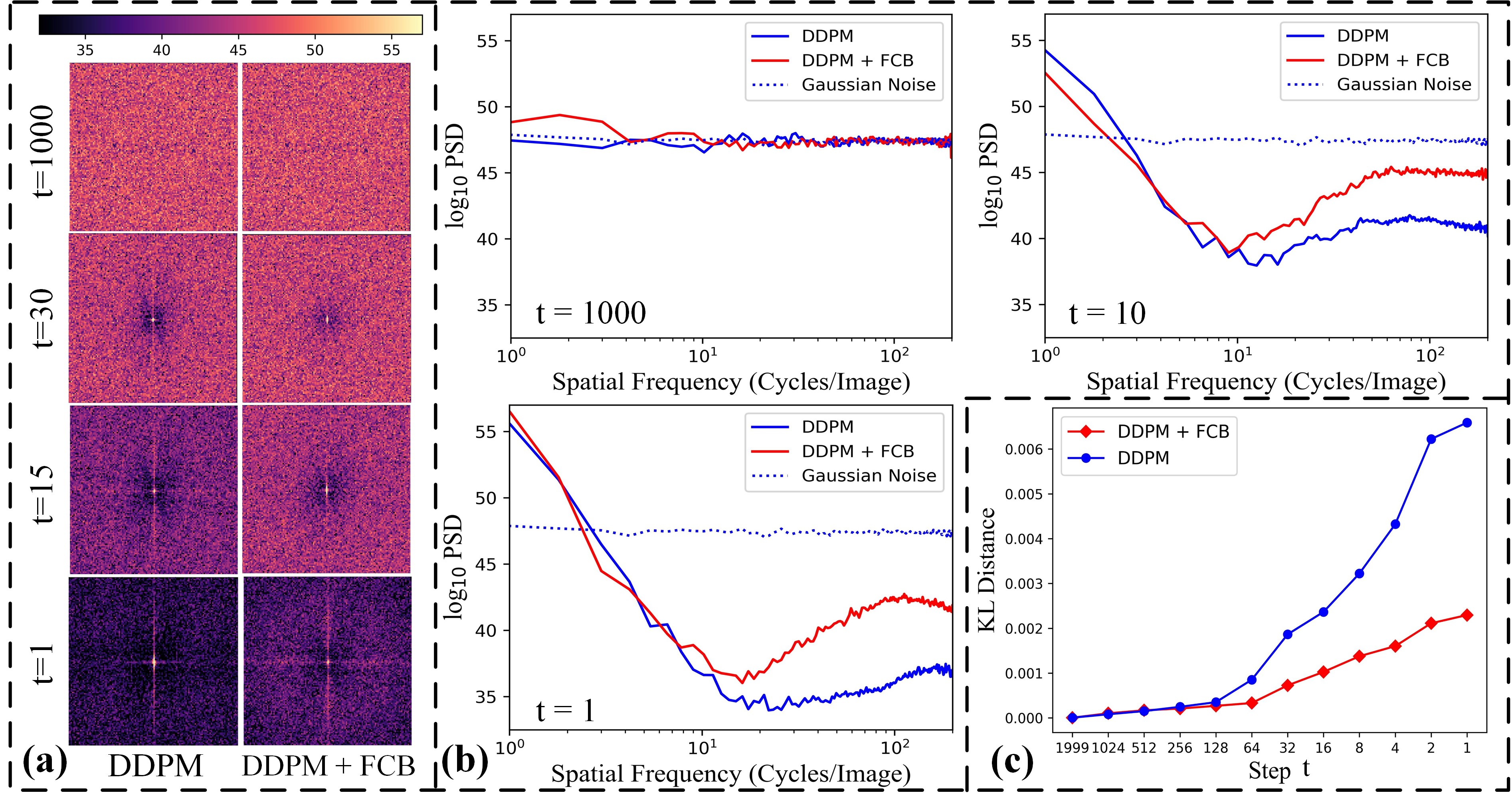
Figure 5: Power spectrum analysis on $\epsilon$-prediction results of DDPMs at varying $t$. (a) The power spectra of DDPM vs. DDPM+FCB. (b) The PSD analysis of DDPM vs. DDPM+FCB. (c) The KL distance between the spectrum of the predicted $\epsilon$ in (b) and that of the groundtruth. The smaller distance, the closer to groundtruth. Additional results are shown in the Appendix B.2.

Effect of frequency compensation. We examine how the proposed FCB helps with training. Fig.5a visually compares the power spectrum [57] of the predicted $\epsilon$ between a plain DDPM and DDPM+FCB. when $t\rightarrow 1$, a considerably larger amount of higher frequency modes can be observed after introducing FCB. This result is consistent with Fig.5b where the PSD analysis is performed on $\epsilon$-prediction. It validates that frequency compensation helps drive the output spectrum towards being uniformly distributed at smaller $t$. In Fig.5c, we further use the KL distance [38] to measure how far the spectrum of the predicted $\epsilon$ in Fig.5b deviates from the groundtruth Gaussian noise. We notice a clear advantage of using FCB to ease the learning process, especially at $t<100$.

Table 4: Ablation study of FCB with varying number of Gaussian kernels. Bold and underline indicate the best and the second-best.

Datasets	k	$\sigma$	SSIM $\uparrow$	CIEDE $\downarrow$	MUSIQ $\uparrow$
I-Haze	-	-	0.536	18.671	60.730
	{ 7 }	{ 10 }	0.731	13.205	64.351
	{ 3,7 }	{ 1,4 }	0.732	12.909	65.372
	{ 3,5,7 }	{ 1,2,4 }	0.747	12.047	65.571
	{ 3,5,7,7 }	{ 1,2,4,15 }	0.754	12.808	65.714
O-Haze	-	-	0.708	18.006	62.241
	{ 7 }	{ 10 }	0.714	16.112	63.098
	{ 3,7 }	{ 1,4 }	0.711	16.103	63.192
	{ 3,5,7 }	{ 1,2,4 }	0.712	15.805	63.463
	{ 3,5,7,7 }	{ 1,2,4,15 }	0.710	15.998	63.094

Ablation of filter design in FCB. We set up different filter configurations to identify the important factors of FCB design. We first vary the number of Gaussian kernels from $M=\{1,2,3,4\}$ and choose $k$ and $\sigma$ in a way that different settings have similar bandwidth. Table 4 shows that even a single high-pass filter leads to a drastic improvement in performance. With more kernels, FCB can more flexibly adapt to training at varying $t$ and hence better performance. However, as the number of filters keeps increasing, the performance gain gradually saturates. We finally choose $M=3$ in this paper as it offers a well trade-off between the performance and computation efficiency. Additional ablation studies of filter design are shown in the Appendix B.3.

Table 5: Ablation study of HazeAug. Bold and underline indicate the best and the second-best, respectively.

Datasets	Augmentation Methods			Indicator
	Traditional	Hard Sample	Haze Migration	SSIM $\uparrow$	CIEDE $\downarrow$	MUSIQ $\uparrow$
I-Haze	$\checkmark$			0.536	18.671	60.730
		$\checkmark$		0.810	14.647	68.341
			$\checkmark$	0.745	15.341	66.164
		$\checkmark$	$\checkmark$	0.812	12.120	68.353
O-Haze	$\checkmark$			0.708	18.006	62.241
		$\checkmark$		0.750	16.314	66.383
			$\checkmark$	0.732	16.487	62.341
		$\checkmark$	$\checkmark$	0.776	15.081	64.219

Ablation of HazeAug. In Table 5, we study the two operators in HazeAug, hard sample and haze migration. Interestingly, although designed to handle severe hazy conditions, such as Dense- and Nh-haze, hard sample also drastically improves the performance on I-Haze and O-Haze. A possible reason is that shielding the clean content from the diffusion models by severe haze forces them to rely less on its visual cues, but encourages them to do more generative modeling.

As for haze migration, we observe considerable improvements across all metrics, especially the reference-based ones. Such distortion reduction can be attributed to the LFC migration, which implicitly forces the model to learn robust high-frequency signals that are invariant to the changing low-frequency ones.

5 Conclusion

We propose a dehazing framework based on conditional diffusion models which demonstrates superior generalization ability to real haze via comprehensive experiments. Specifically, we design a novel network unit, FCB, to ease the learning and provide insights into the limitation of diffusion models in restoring high-frequency image details. We hope it may prove useful for other inverse problems. Then, we find that diffusion models significantly benefit from effectively augmented data for improved generality. It shows potential of diffusion models to handle challenging issues (e.g., heterogeneous haze, color distortion) if applied with more sophisticated haze augmentation.

6 Acknowledgement

All the work is done at Sony R & D Center China, Beijing Lab, supported by Sony Research Fund from June 2022 to May 2023.

References

- [1] Cosmin Ancuti, Codruta O Ancuti, Radu Timofte, and Christophe De Vleeschouwer. I-haze: a dehazing benchmark with real hazy and haze-free indoor images. In International Conference on Advanced Concepts for Intelligent Vision Systems, pages 620–631. Springer, 2018.
- [2] Codruta O Ancuti, Cosmin Ancuti, Mateu Sbert, and Radu Timofte. Dense-haze: A benchmark for image dehazing with dense-haze and haze-free images. In 2019 IEEE international conference on image processing (ICIP), pages 1014–1018. IEEE, 2019.
- [3] Codruta O Ancuti, Cosmin Ancuti, and Radu Timofte. Nh-haze: An image dehazing benchmark with non-homogeneous hazy and haze-free images. In Proceedings of the IEEE/CVF conference on computer vision and pattern recognition workshops, pages 444–445, 2020.
- [4] Codruta O Ancuti, Cosmin Ancuti, Radu Timofte, and Christophe De Vleeschouwer. O-haze: a dehazing benchmark with real hazy and haze-free outdoor images. In Proceedings of the IEEE conference on computer vision and pattern recognition workshops, pages 754–762, 2018.
- [5] Omri Avrahami, Dani Lischinski, and Ohad Fried. Blended diffusion for text-driven editing of natural images. In Proceedings of the IEEE/CVF Conference on Computer Vision and Pattern Recognition, pages 18208–18218, 2022.
- [6] Haoran Bai, Jinshan Pan, Xinguang Xiang, and Jinhui Tang. Self-guided image dehazing using progressive feature fusion. IEEE Transactions on Image Processing, 31:1217–1229, 2022.
- [7] Dana Berman, Shai Avidan, et al. Non-local image dehazing. In Proceedings of the IEEE conference on computer vision and pattern recognition, pages 1674–1682, 2016.
- [8] Glenn D Boreman. Modulation transfer function in optical and electro-optical systems, volume 4. SPIE press Bellingham, Washington, 2001.
- [9] Trung Minh Bui and Wonha Kim. Single image dehazing using color ellipsoid prior. IEEE Transactions on Image Processing, 27(2):999–1009, 2017.
- [10] Alan Bundy and Lincoln Wallen. Difference of gaussians. Catalogue of Artificial Intelligence Tools, pages 30–30, 1984.
- [11] Bolun Cai, Xiangmin Xu, Kui Jia, Chunmei Qing, and Dacheng Tao. Dehazenet: An end-to-end system for single image haze removal. IEEE Transactions on Image Processing, 25(11):5187–5198, 2016.
- [12] Dongdong Chen, Mingming He, Qingnan Fan, Jing Liao, Liheng Zhang, Dongdong Hou, Lu Yuan, and Gang Hua. Gated context aggregation network for image dehazing and deraining. In 2019 IEEE winter conference on applications of computer vision (WACV), pages 1375–1383. IEEE, 2019.
- [13] Guangyao Chen, Peixi Peng, Li Ma, Jia Li, Lin Du, and Yonghong Tian. Amplitude-phase recombination: Rethinking robustness of convolutional neural networks in frequency domain. In Proceedings of the IEEE/CVF International Conference on Computer Vision, pages 458–467, 2021.
- [14] Zeyuan Chen, Yangchao Wang, Yang Yang, and Dong Liu. Psd: Principled synthetic-to-real dehazing guided by physical priors. In Proceedings of the IEEE/CVF conference on computer vision and pattern recognition, pages 7180–7189, 2021.
- [15] Prafulla Dhariwal and Alexander Nichol. Diffusion models beat gans on image synthesis. Advances in Neural Information Processing Systems, 34:8780–8794, 2021.
- [16] Hang Dong, Jinshan Pan, Lei Xiang, Zhe Hu, Xinyi Zhang, Fei Wang, and Ming-Hsuan Yang. Multi-scale boosted dehazing network with dense feature fusion. In Proceedings of the IEEE/CVF conference on computer vision and pattern recognition, pages 2157–2167, 2020.
- [17] Yu Dong, Yihao Liu, He Zhang, Shifeng Chen, and Yu Qiao. Fd-gan: Generative adversarial networks with fusion-discriminator for single image dehazing. In Proceedings of the AAAI Conference on Artificial Intelligence, volume 34, pages 10729–10736, 2020.
- [18] Alexey Dosovitskiy, Lucas Beyer, Alexander Kolesnikov, Dirk Weissenborn, Xiaohua Zhai, Thomas Unterthiner, Mostafa Dehghani, Matthias Minderer, Georg Heigold, Sylvain Gelly, et al. An image is worth 16x16 words: Transformers for image recognition at scale. arXiv preprint arXiv:2010.11929, 2020.
- [19] Deniz Engin, Anil Genç, and Hazim Kemal Ekenel. Cycle-dehaze: Enhanced cyclegan for single image dehazing. In Proceedings of the IEEE conference on computer vision and pattern recognition workshops, pages 825–833, 2018.
- [20] Raanan Fattal. Dehazing using color-lines. ACM transactions on graphics (TOG), 34(1):1–14, 2014.
- [21] Clément Godard, Oisin Mac Aodha, and Gabriel J. Brostow. Unsupervised monocular depth estimation with left-right consistency. In CVPR, 2017.
- [22] Ian Goodfellow, Jean Pouget-Abadie, Mehdi Mirza, Bing Xu, David Warde-Farley, Sherjil Ozair, Aaron Courville, and Yoshua Bengio. Generative adversarial networks. Communications of the ACM, 63(11):139–144, 2020.
- [23] Kaiming He, Xinlei Chen, Saining Xie, Yanghao Li, Piotr Dollár, and Ross Girshick. Masked autoencoders are scalable vision learners. In Proceedings of the IEEE/CVF Conference on Computer Vision and Pattern Recognition, pages 16000–16009, 2022.
- [24] Kaiming He, Jian Sun, and Xiaoou Tang. Single image haze removal using dark channel prior. IEEE transactions on pattern analysis and machine intelligence, 33(12):2341–2353, 2010.
- [25] Jonathan Ho, Ajay Jain, and Pieter Abbeel. Denoising diffusion probabilistic models. Advances in Neural Information Processing Systems, 33:6840–6851, 2020.
- [26] Jonathan Ho and Tim Salimans. Classifier-free diffusion guidance. arXiv preprint arXiv:2207.12598, 2022.
- [27] Alain Hore and Djemel Ziou. Image quality metrics: Psnr vs. ssim. In 2010 20th international conference on pattern recognition, pages 2366–2369. IEEE, 2010.
- [28] Heewoo Jun, Rewon Child, Mark Chen, John Schulman, Aditya Ramesh, Alec Radford, and Ilya Sutskever. Distribution augmentation for generative modeling. In International Conference on Machine Learning, pages 5006–5019. PMLR, 2020.
- [29] Junjie Ke, Qifei Wang, Yilin Wang, Peyman Milanfar, and Feng Yang. Musiq: Multi-scale image quality transformer. In Proceedings of the IEEE/CVF International Conference on Computer Vision, pages 5148–5157, 2021.
- [30] Boyi Li, Xiulian Peng, Zhangyang Wang, Jizheng Xu, and Dan Feng. Aod-net: All-in-one dehazing network. In Proceedings of the IEEE international conference on computer vision, pages 4770–4778, 2017.
- [31] Boyi Li, Wenqi Ren, Dengpan Fu, Dacheng Tao, Dan Feng, Wenjun Zeng, and Zhangyang Wang. Benchmarking single-image dehazing and beyond. IEEE Transactions on Image Processing, 28(1):492–505, 2018.
- [32] Chongyi Li, Chunle Guo, Jichang Guo, Ping Han, Huazhu Fu, and Runmin Cong. Pdr-net: Perception-inspired single image dehazing network with refinement. IEEE Transactions on Multimedia, 22(3):704–716, 2019.
- [33] Chongyi Li, Jichang Guo, Fatih Porikli, Chunle Guo, Huzhu Fu, and Xi Li. Dr-net: transmission steered single image dehazing network with weakly supervised refinement. arXiv preprint arXiv:1712.00621, 2017.
- [34] Wei Liu, Xianxu Hou, Jiang Duan, and Guoping Qiu. End-to-end single image fog removal using enhanced cycle consistent adversarial networks. IEEE Transactions on Image Processing, 29:7819–7833, 2020.
- [35] Yang Liu, Jinshan Pan, Jimmy Ren, and Zhixun Su. Learning deep priors for image dehazing. In Proceedings of the IEEE/CVF international conference on computer vision, pages 2492–2500, 2019.
- [36] Ye Liu, Lei Zhu, Shunda Pei, Huazhu Fu, Jing Qin, Qing Zhang, Liang Wan, and Wei Feng. From synthetic to real: Image dehazing collaborating with unlabeled real data. In Proceedings of the 29th ACM International Conference on Multimedia, pages 50–58, 2021.
- [37] Chenlin Meng, Yang Song, Jiaming Song, Jiajun Wu, Jun-Yan Zhu, and Stefano Ermon. Sdedit: Image synthesis and editing with stochastic differential equations. arXiv preprint arXiv:2108.01073, 2021.
- [38] Kevin P Murphy. Machine learning: a probabilistic perspective. MIT press, 2012.
- [39] Shree K Nayar and Srinivasa G Narasimhan. Vision in bad weather. In Proceedings of the seventh IEEE international conference on computer vision, volume 2, pages 820–827. IEEE, 1999.
- [40] Ko Nishino, Louis Kratz, and Stephen Lombardi. Bayesian defogging. International journal of computer vision, 98:263–278, 2012.
- [41] Xu Qin, Zhilin Wang, Yuanchao Bai, Xiaodong Xie, and Huizhu Jia. Ffa-net: Feature fusion attention network for single image dehazing. In Proceedings of the AAAI Conference on Artificial Intelligence, volume 34, pages 11908–11915, 2020.
- [42] Nasim Rahaman, Aristide Baratin, Devansh Arpit, Felix Draxler, Min Lin, Fred Hamprecht, Yoshua Bengio, and Aaron Courville. On the spectral bias of neural networks. In International Conference on Machine Learning, pages 5301–5310. PMLR, 2019.
- [43] Zia-ur Rahman, Daniel J Jobson, and Glenn A Woodell. Multi-scale retinex for color image enhancement. In Proceedings of 3rd IEEE international conference on image processing, volume 3, pages 1003–1006. IEEE, 1996.
- [44] AJ Rainal. Sampling technique for generating gaussian noise. Review of Scientific Instruments, 32(3):327–331, 1961.
- [45] Olaf Ronneberger, Philipp Fischer, and Thomas Brox. U-net: Convolutional networks for biomedical image segmentation. In International Conference on Medical image computing and computer-assisted intervention, pages 234–241. Springer, 2015.
- [46] Chitwan Saharia, William Chan, Huiwen Chang, Chris Lee, Jonathan Ho, Tim Salimans, David Fleet, and Mohammad Norouzi. Palette: Image-to-image diffusion models. In ACM SIGGRAPH 2022 Conference Proceedings, pages 1–10, 2022.
- [47] Chitwan Saharia, Jonathan Ho, William Chan, Tim Salimans, David J Fleet, and Mohammad Norouzi. Image super-resolution via iterative refinement. arXiv preprint arXiv:2104.07636, 2021.
- [48] Chitwan Saharia, Jonathan Ho, William Chan, Tim Salimans, David J Fleet, and Mohammad Norouzi. Image super-resolution via iterative refinement. IEEE Transactions on Pattern Analysis and Machine Intelligence, 2022.
- [49] Yuanjie Shao, Lerenhan Li, Wenqi Ren, Changxin Gao, and Nong Sang. Domain adaptation for image dehazing. In Proceedings of the IEEE/CVF conference on computer vision and pattern recognition, pages 2808–2817, 2020.
- [50] Gaurav Sharma, Wencheng Wu, and Edul N Dalal. The ciede2000 color-difference formula: Implementation notes, supplementary test data, and mathematical observations. Color Research & Application: Endorsed by Inter-Society Color Council, The Colour Group (Great Britain), Canadian Society for Color, Color Science Association of Japan, Dutch Society for the Study of Color, The Swedish Colour Centre Foundation, Colour Society of Australia, Centre Français de la Couleur, 30(1):21–30, 2005.
- [51] Hamid R Sheikh, Alan C Bovik, and Lawrence Cormack. No-reference quality assessment using natural scene statistics: Jpeg2000. IEEE Transactions on image processing, 14(11):1918–1927, 2005.
- [52] Jascha Sohl-Dickstein, Eric Weiss, Niru Maheswaranathan, and Surya Ganguli. Deep unsupervised learning using nonequilibrium thermodynamics. In International Conference on Machine Learning, pages 2256–2265. PMLR, 2015.
- [53] Jiaming Song, Chenlin Meng, and Stefano Ermon. Denoising diffusion implicit models. arXiv preprint arXiv:2010.02502, 2020.
- [54] Yang Song and Stefano Ermon. Generative modeling by estimating gradients of the data distribution. Advances in Neural Information Processing Systems, 32, 2019.
- [55] Yuda Song, Zhuqing He, Hui Qian, and Xin Du. Vision transformers for single image dehazing. arXiv preprint arXiv:2204.03883, 2022.
- [56] Yang Song, Liyue Shen, Lei Xing, and Stefano Ermon. Solving inverse problems in medical imaging with score-based generative models. arXiv preprint arXiv:2111.08005, 2021.
- [57] Milan Sonka, Vaclav Hlavac, and Roger Boyle. Image processing, analysis, and machine vision. Cengage Learning, 2014.
- [58] Alexander Tanchenko. Visual-psnr measure of image quality. Journal of Visual Communication and Image Representation, 25(5):874–878, 2014.
- [59] Ketan Tang, Jianchao Yang, and Jue Wang. Investigating haze-relevant features in a learning framework for image dehazing. In Proceedings of the IEEE conference on computer vision and pattern recognition, pages 2995–3000, 2014.
- [60] van A Van der Schaaf and JH van van Hateren. Modelling the power spectra of natural images: statistics and information. Vision research, 36(17):2759–2770, 1996.
- [61] Cong Wang, Yan Huang, Yuexian Zou, and Yong Xu. Fully non-homogeneous atmospheric scattering modeling with convolutional neural networks for single image dehazing. arXiv preprint arXiv:2108.11292, 2021.
- [62] Cong Wang, Yan Huang, Yuexian Zou, and Yong Xu. Fwb-net: front white balance network for color shift correction in single image dehazing via atmospheric light estimation. In ICASSP 2021-2021 IEEE International Conference on Acoustics, Speech and Signal Processing (ICASSP), pages 2040–2044. IEEE, 2021.
- [63] Haohan Wang, Xindi Wu, Zeyi Huang, and Eric P Xing. High-frequency component helps explain the generalization of convolutional neural networks. In Proceedings of the IEEE/CVF Conference on Computer Vision and Pattern Recognition, pages 8684–8694, 2020.
- [64] Zhou Wang, Alan C Bovik, Hamid R Sheikh, and Eero P Simoncelli. Image quality assessment: from error visibility to structural similarity. IEEE transactions on image processing, 13(4):600–612, 2004.
- [65] Zhou Wang, Eero P Simoncelli, and Alan C Bovik. Multiscale structural similarity for image quality assessment. In The Thrity-Seventh Asilomar Conference on Signals, Systems & Computers, 2003, volume 2, pages 1398–1402. Ieee, 2003.
- [66] Stephen Westland, Caterina Ripamonti, and Vien Cheung. Computational colour science using MATLAB. John Wiley & Sons, 2012.
- [67] Jay Whang, Mauricio Delbracio, Hossein Talebi, Chitwan Saharia, Alexandros G. Dimakis, and Peyman Milanfar. Deblurring via stochastic refinement. In Proceedings of the IEEE/CVF Conference on Computer Vision and Pattern Recognition (CVPR), pages 16293–16303, June 2022.
- [68] Haoran Xu, Jianming Guo, Qing Liu, and Lingli Ye. Fast image dehazing using improved dark channel prior. In 2012 IEEE international conference on information science and technology, pages 663–667. IEEE, 2012.
- [69] Yanchao Yang and Stefano Soatto. Fda: Fourier domain adaptation for semantic segmentation. In Proceedings of the IEEE/CVF Conference on Computer Vision and Pattern Recognition, pages 4085–4095, 2020.
- [70] He Zhang and Vishal M Patel. Densely connected pyramid dehazing network. In Proceedings of the IEEE conference on computer vision and pattern recognition, pages 3194–3203, 2018.
- [71] Xi Zhao, Keyan Wang, Yunsong Li, and Jiaojiao Li. Deep fully convolutional regression networks for single image haze removal. In 2017 IEEE Visual Communications and Image Processing (VCIP), pages 1–4. IEEE, 2017.
- [72] Jun-Yan Zhu, Taesung Park, Phillip Isola, and Alexei A Efros. Unpaired image-to-image translation using cycle-consistent adversarial networks. In Proceedings of the IEEE international conference on computer vision, pages 2223–2232, 2017.
- [73] Qingsong Zhu, Jiaming Mai, and Ling Shao. A fast single image haze removal algorithm using color attenuation prior. IEEE transactions on image processing, 24(11):3522–3533, 2015.