Distributions and Physical Properties of Molecular Clouds in the Third Galactic Quadrant: $l=[\,219\fdg 75,~{}229\fdg 75\,]$ and $b=[\,-5\fdg 25,~{}5\fdg 25\,]$

Abstract

We present the results of an unbiased ¹²CO/¹³CO/C¹⁸O ($J=1$–0) survey in a portion of the third Galactic quadrant (TGQ): $219\fdg 75\leqslant l\leqslant 229\fdg 75$ and $-5\fdg 25\leqslant b\leqslant 5\fdg 25$. The high-resolution and high-sensitivity data sets help to unravel the distributions and physical properties of the molecular clouds (MCs) in the mapped area. In the LSR velocity range from $\sim$$-1$ to $\sim$$85~{}\rm km\,s^{-1}$, the molecular material successfully traces the Local, Perseus, and Outer arms. In the TGQ, the Outer arm appears to be more prominent than that in the second Galactic quadrant (SGQ), but the Perseus arm is not as conspicuous as that in the SGQ. A total of 1,502 ¹²CO, 570 ¹³CO, and 53 C¹⁸O molecular structures are identified, spanning over $\sim$2 and $\sim$6 orders of magnitude in size and mass, respectively. Tight mass–radius correlations and virial parameter–mass anticorrelations are observable. Yet, it seems that no clear correlations between velocity dispersion and effective radius can be found over the full dynamic range. The vertical distribution of the MCs renders evident pictures of the Galactic warp and flare.

1 Introduction

Table 1: CO Surveys of the TGQ

Telescope	Transitions	Sky	Beam	Velocity	RMS	Reference
	($J=1$–0)	Coverage	Size	Resolution	Noise
				($\rm km\,s^{-1}$)	($T\rm_{MB}$)(K)
CfA 1.2 m	12CO	All Galactic plane	$8\farcm 8$	1.3	0.1–0.4	(1)
		$194\degree\leqslant l\leqslant 270\degree$,				(2)
		$-4\degree\leqslant b\leqslant 1\degree$
NANTEN 4 m	12CO	$220\degree\leqslant l\leqslant 60\degree$,	$2\farcm 6$	0.65	0.4	(3)
		$|b|\leqslant 10\degree$
Nagoya 4 m	13CO	$208\degree\leqslant l\leqslant 230\degree$,	$2\farcm 7$	0.1	0.5	(4)
		$-20\degree\leqslant b\leqslant 10\degree$
Mopra 22 m	12CO/13CO/	$l\sim 224\fdg 4$,	$\sim$$38\arcsec$	$\sim$0.1	0.3–0.9	(5)
	C18O/C17O	$b\sim-0\fdg 6$
Nobeyama 45 m	12CO/13CO/	$10\degree\leqslant l\leqslant 50\degree$; $198\degree\leqslant l\leqslant 236\degree$,	$\sim$$14\arcsec$	$\sim$1.3	0.6/0.3	(6)
	C18O	$|b|\leqslant 1\degree$
ARO 12 m	12CO/13CO	$220\degree<l<240\degree$,	$\sim$$55\arcsec$	0.26/0.65	0.3–1.3	(7)
		$-2\fdg 5<b<0\degree$
PMO 13.7-m	12CO/13CO/	$10\degree\lesssim l\lesssim 230\degree$,	$\sim$$50\arcsec$	$\sim$0.16	0.5/0.3	(8)
	C18O	$|b|\leqslant 5\fdg 25$

References. — (1) Dame et al. (1987, 2001); (2) May et al. (1993, 1997); (3) Mizuno & Fukui (2004); (4) Kim et al. (2004); (5) Olmi et al. (2016); (6) Umemoto et al. (2017); (7) Benedettini et al. (2020, 2021); and (8) Su et al. (2019).

CO has been the most commonly used tracer of the molecular gas since its first detection (Wilson et al., 1970), and numerous CO line surveys have been conducted over the decades (Heyer & Dame, 2015, and references therein). Unlike the first quadrant of the Galaxy, the third Galactic quadrant (TGQ) has neither been extensively observed nor widely discussed. Table 1 summarizes the CO surveys of the TGQ. Using the CfA 1.2 m survey data, Rice et al. (2016) and Miville-Deschênes et al. (2017) produced their individual all-Galaxy molecular cloud (MC) catalogs by applying different cloud detection algorithms. Combining the ¹²CO data of Mizuno & Fukui (2004) with Herschel data, Elia et al. (2013) studied the star formation activity in the TGQ. More recently, Benedettini et al. (2020, 2021) have studied the large-scale molecular material distributions and properties in this region by using the Forgotten Quadrant Survey’s ¹²CO and ¹³CO (1–0) line data, which were conducted by the Arizona Radio Observatory (ARO) $12\rm~{}m$ antenna. Although our knowledge of the molecular interstellar medium has improved, new data, with the combination of multitracers, high-sensitivity, high-resolution, and wide Galactic coverage, can offer more accurate and comprehensive insights into the TGQ.

Such data are currently being provided by the ongoing Milky Way Imaging Scroll Painting (MWISP) project, an unbiased large-scale ¹²CO, ¹³CO, and C¹⁸O ($J=1$–0) survey conducted by the Purple Mountain Observatory (PMO) 13.7 m telescope (Su et al., 2019). To date, the Galactic range of $l=[\,219\fdg 75,~{}229\fdg 75\,]$ and $b=[\,-5\fdg 25,~{}5\fdg 25\,]$ (hereafter, the G220 region) has been fully mapped by the MWISP project. This study aims to investigate the essential information of the spatial distribution and physical properties of MCs in the G220 region. The entire G220 region covers a total of 105 deg², which contains several well-separated spiral arm features (the Local, Perseus, and Outer arms) along the line of sight. The high-quality MWISP data can provide a more comprehensive cloud sample than previous studies, especially for the Outer arm. Therefore, we can expect to reveal new features of the molecular gas distribution within this region.

In this paper, we present the results of the MWISP ¹²CO/¹³CO/C¹⁸O ($J=1$–0) survey toward the G220 region ($J=1$–0 may be omitted hereafter, for simplicity). In Section 2, we summarize the observations, data reduction, and cloud identification. In Section 3.1, we present the large-scale structures traced by ¹²CO, ¹³CO, and C¹⁸O data. Estimates of and statistics for the physical properties are exhibited from Sections 3.2 to 3.4. Section 3.5 describes five particular MCs. Spatial distributions of the MCs are shown in Section 4. A summary can be found in Section 5.

2 Data

2.1 Observations and Data Reduction

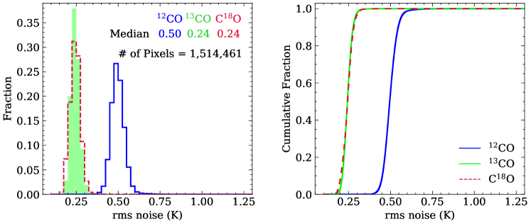
Figure 1: Left: histograms of the rms noise levels ($\sigma$) for ¹²CO (blue), ¹³CO (green), and C¹⁸O (red). The median values of $\sigma$ and the total number of pixels are marked in the top right corner. Right: cumulative distributions of $\sigma$.

The observations were conducted from 2016 December to 2021 April by using the PMO $13.7~{}\rm m$ millimeter-wavelength telescope in Delingha, China. The telescope, with a half-power beam width of $\sim$$50\arcsec$ at $115\rm~{}GHz$, operates with a $3\times 3$ multibeam sideband separation receiver named the Superconducting Spectroscopic Array Receiver (Yang et al., 2008; Shan et al., 2012). The backend of the receiver system comprises 18 fast Fourier transform spectrometers, each configured with $1\rm~{}GHz$ bandwidth and 16,384 spectral channels, which yield a velocity coverage of $\sim$2,600$\rm~{}km\,s^{-1}$, and yield velocity resolutions of $0.159\rm~{}km\,s^{-1}$ at $115\rm~{}GHz$ and $0.166\rm~{}km\,s^{-1}$ at $110\rm~{}GHz$. The ¹²CO line is observed at the upper sideband, while the ¹³CO and C¹⁸O lines are observed at the lower sideband simultaneously.

The G220 region is divided into 420 small tiles for the on-the-fly (OTF) mapping, each with a size of $30\arcmin\times 30\arcmin$. The CLASS software from the GILDAS package (Pety, 2005) is used for data reduction. The OTF data are resampled into $30\arcsec\times 30\arcsec$ pixels and converted to three-dimensional (3D) FITS cubes after a first-order baseline is applied to the spectra. The velocity channels are not smoothed. The data in the FITS cubes are on the main-beam brightness temperature ($T_{\rm MB}$) scale, which is converted from the antenna temperature ($T^{\ast}_{\rm A}$) with the typical beam efficiencies of $\sim$0.51 for ¹³CO and C¹⁸O and $\sim$0.46 for ¹²CO (see the status report of the telescope). Adding the 420 tiles together, we create the final large mosaic, which contains 1,514,461 spectra for each CO isotopolog. Please also refer to Su et al. (2019) for more details about the observations and data reduction. Figure 1 shows the normalized distributions of rms noise levels for ¹²CO (blue), ¹³CO (green), and C¹⁸O (red). The median rms noise values are $\sim$$0.50\rm~{}K$ for ¹²CO at a channel width of $\sim$$0.16\rm~{}km\,s^{-1}$, and $\sim$$0.24\rm~{}K$ for ¹³CO and C¹⁸O at a channel width of $\sim$$0.17\rm~{}km\,s^{-1}$.

2.2 Cloud Identification and Bad Channel Cleaning

An MC is popularly defined as a set of contiguous voxels in the position-position-velocity (PPV) space, with the brightness temperatures above a threshold (Heyer & Dame, 2015). Based on this definition, we employ an approach developed by Yan et al. (2020) to identify the molecular structures from the ¹²CO, ¹³CO, and C¹⁸O data. Note that the identified ¹²CO structures are often referred to as ¹²CO clouds or MCs. The technique is based on the density-based spatial clustering of applications with noise (DBSCAN) algorithm (Ester et al., 1996), which contains three free parameters: $\epsilon$ and MinPts define the connection property of the voxels in the PPV space, while $T_{\rm cutoff}$ defines the boundary isosurface of the structures (Yan et al., 2020). A judicious option is $\epsilon=1$, $\rm MinPts=4$, and $T_{\rm cutoff}=2\sigma$, ensuring most of the significant emission being identified without omitting the faint but real signals. Yan et al. (2020) also recommend the usage of post-selection criteria to exclude the noise and bad channel contamination as much as possible. A sample will be rejected from the raw catalog if it does not meet the following criteria: (1) number of voxels $\geqslant 16$; (2) peak main-beam brightness temperature $\geqslant 5\sigma$; (3) projection area contains more than one compact $2\times 2$ pixels ($1\arcmin\times 1\arcmin$ area); and (4) the number of velocity channels $\geqslant 3$.

We then apply the DBSCAN signal identification results to mask the raw data cubes. However, we see that the bad channels centered at $\sim$$34~{}\rm km\,s^{-1}$ with a typical width of four to five channels (see Figure A1 in Appendix A) cannot be completely excluded by the post-selection criteria. Therefore, we visually inspect all identified structures based on their spatial and velocity features in the PPV space. Fortunately, we find that the bad channels contaminate only three real MCs (MWISP G224.153$+$1.211, MWISP G223.784$+$2.950, and MWISP G224.097$+$2.290, marked as the red circles in Figures 2, 3, and A1), while the majority of the bad channels simply produce spurious samples that contain only bad channels without the presence of real signal and show no signs of hierarchical structures. To get rid of the effects of these bad channels, we further exclude the spurious samples to make the final catalog (see Table B1 in Appendix B), and ignore the three contaminated ¹²CO clouds as well as their associated ¹³CO structure (MWISP G224.166$+$1.218) when estimating physical properties.

Table 2: Number of Samples

Layer	Emission	Full	Flawed	Sliced	Counted
Name	Line	Sample	Sample	Sample	Sample
Local Arm	12CO	830	0	6	824
	13CO	419	0	1	418
	C18O	48	0	0	48
Perseus Arm	12CO	404	3	6	395
	13CO	112	1	0	111
	C18O	5	0	0	5
Outer Arm	12CO	268	0	4	264
	13CO	39	0	1	38

Note. — “Full Sample” in Column 3 includes all confident samples in our catalog. Column 4, “Flawed Sample”, gives the number of samples contaminated by the bad channels (see Section 2.2). Note that one of the contaminated ¹²CO clouds contains a ¹³CO structure that is also treated as a contaminated sample. Column 5, “Sliced Sample”, lists the number of samples that touch the mapped borders. These structures are truncated by the edges of the G220 region, leaving less than half of the complete molecular structures. By subtracting Columns 4 and 5 from Column 3, we get Column 6 (“Counted Sample”), the number of samples that are used for the analysis of physical properties (see Sections 3.3.2, 3.3.3 and 3.4).

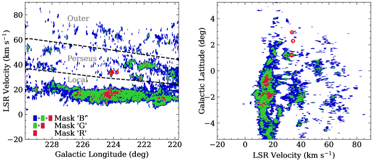
Figure 2: Longitude–velocity (left) and latitude–velocity (right) maps of the “cleaned” CO emission, integrated over a Galactic latitude range from $-5\fdg 25$ to $5\fdg 25$ and a Galactic longitude range from $219\fdg 75$ to $229\fdg 75$, respectively. The maps only contain emission from the samples in our catalog. Mask “B,” “G,” and “R” indicate the regions where ¹²CO, ¹³CO, and C¹⁸O emission exists, respectively. The three contaminated MCs are marked as the red circles. The dashed lines sketch out the boundaries of each velocity layer.

3 Results

3.1 Large-scale Structures Traced by ${}^{12}{\rm CO}$, ${}^{13}{\rm CO}$, and ${\rm C}^{18}{\rm O}$

The number of samples is listed in Table 2. In total, we detected 1,502 ¹²CO, 570 ¹³CO, and 53 C¹⁸O molecular structures. One can see that the number of the ¹²CO structures of the Local arm is more than twice that of the Perseus arm and more than three times that of the Outer arm. Figure 2 displays the “cleaned” $l$–$v$ and $b$–$v$ diagrams, i.e., only containing emission from the confident molecular structures identified by this study. Following Sun et al. (2020), we define the mask “B,” “G,” and “R” regions as the regions where ¹²CO, ¹³CO, and C¹⁸O emission exists, respectively. Note that the mask “R” region contains ¹²CO and ¹³CO emission, and the mask “G” region contains ¹²CO emission as well. According to this definition, the red mask “R” region in Figure 2 is included in the green mask “G” region, and the latter is further included in the blue mask “B” region.

We find that the molecular gas emission is located in the LSR velocity ($v\rm_{\scriptscriptstyle LSR}$) range from $\sim$$-1$ to $\sim$$85~{}\rm km\,s^{-1}$ in Figure 2. The dashed lines are defined as the boundaries that have the same velocity separation to the adjacent arm centers (refer to Figure 3 of Reid et al., 2019). It is intriguing that the new high-quality MWISP data successfully trace not only the two nearby spiral arms, but also the distant Outer arm. However, from the $b$–$v$ map, it seems that our current Galactic latitude coverage is still very limited in revealing a complete view of the Local arm. Also note that we do not subdivide the interarm regions since their contribution to the total emission is quite small.

The mask maps of integrated intensity of the whole G220 region and the three arm features therein are shown in Figure 3, where the mask “B,” “G,” and “R” regions are defined the same as in Figure 2. We see that both ¹²CO and ¹³CO emission are detected in all velocity layers, while C¹⁸O emission is only present in the two more nearby spiral arms at our current sensitivities. The decrease in flux completeness with the increasing distance may largely account for the nondetection of C¹⁸O emission in the Outer arm.

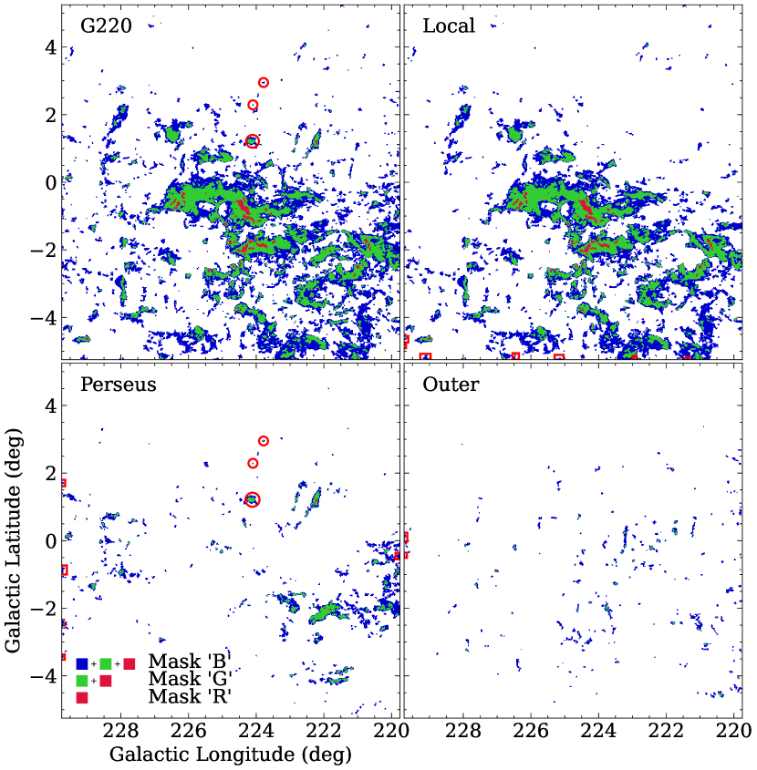
Figure 3: Mask regions of the entire G220 region (top-left) and the Local (top-right), Perseus (bottom-left), and Outer (bottom-right) arms. The definitions of the mask “B,” “G,” and “R” regions are the same as in Figure 2. The red circles and rectangles mark the structures that are contaminated by bad channels and touch the borders of the G220 region, respectively. These structures will be ignored in the statistical analysis.

Table 3: Layers and Mask Regions

Layer	Mask	Pixel	Pixel
Name	Region	Number	Percentage
Local Arm	B	244,729	16.2$\%$
	G	83,004	5.5$\%$
	R	4,176	0.3$\%$
Perseus Arm	B	41,999	2.8$\%$
	G	8,712	0.6$\%$
	R	123	0.008%
Outer Arm	B	13,066	0.9$\%$
	G	1,071	0.07$\%$

Note. — Pixel percentage is defined as the ratio of the pixel number in each mask region to the total number of pixels in the G220 region, i.e., 1,514,461.

The pixel numbers and pixel percentages (the ratios of pixel numbers to the total pixel number in the entire map, i.e., 1,514,461) of the mask regions are listed in Table 3. Obviously, only a small fraction ($\lesssim$16.2%) of the mapped pixels show CO emission, and the pixel percentages decrease rapidly from the nearest arm to the farthest arm. However, CO emission seems to occupy most of the mapped area in the inner Galaxy, e.g., in the Galactic longitude of $l=[25\fdg 8$, $49\fdg 7$] (see Figure 6 of Su et al., 2019). In the second Galactic quadrant (SGQ), Du et al. (2017) and Sun et al. (2020) also reported pixel percentages of $\lesssim$26.2% and $\lesssim$35.7% in the G140 region ($139\fdg 75\leqslant l\leqslant 149\fdg 25$) and the G130 region ($129\fdg 75\leqslant l\leqslant 140\fdg 25$), respectively. Since all of these studies used the MWISP survey data with uniform quality and employed very similar statistical methods, the differences strongly imply that, on average, the molecular gas becomes sparser when moving from the inner to the outer Galaxy. In addition, as expected, the number of pixels in the mask “B” region is the largest, while that in the mask “R” region is the smallest in each spiral arm layer.

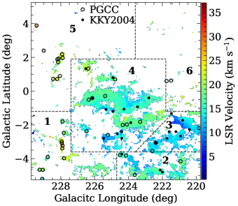
Figure 4: The velocity distribution of ¹²CO in the Local arm. The dashed lines indicate the boundaries of the six regions where different distances were adopted. The cold clumps (empty circles) of the Planck Collaboration et al. (2016) and the ¹³CO clouds (filled circles) of Kim et al. (2004) are used as references for determining the distances in the six regions.

3.2 Distances to MCs

The distances to the MCs in the outer Galactic plane are widely determined by assuming a rotation curve, the so-called kinematic method. However, this method is limited by large uncertainties for nearby clouds. Therefore, for the MCs in the Local arm, we adopt the distances from the literature that are mainly determined by the dust extinction and photometric methods. These methods generally provide more reliable distance measurements than the kinematic method. The Planck Collaboration et al. (2016) estimated the distances of the cold clumps (the empty circles in Figure 4) using the extinction method. Kim et al. (2004) zonally determined the distances of the ¹³CO clouds (the filled circles in Figure 4) in the Canis Major region. Accordingly, the Local arm can be divided into six regions by the dashed lines in Figure 4. For simplicity, we assign a constant distance for the MCs within each region. The adopted distance and the number of MCs in each region are given in Table 3.2. Region 1 is tentatively further subdivided into two cases: a distance of $\rm 0.2~{}kpc$ is adopted for the relatively nearby clouds with low $v\rm_{\scriptscriptstyle LSR}$ (the uncertainty-weighted average distance of the cold clumps in this region; Planck Collaboration et al., 2016), and a distance of $\rm 2~{}kpc$ is adopted for the relatively distant clouds with high $v\rm_{\scriptscriptstyle LSR}$ (Montillaud et al., 2015). Also using the uncertainty-weighted average method, the distances to the MCs in regions 2, 5, and 6 are determined as 0.6, 0.3, and $\rm 0.7~{}kpc$, respectively. Referring to Kim et al. (2004), we assign 1 and $\rm 1.15~{}kpc$ (the photometric distance to the CMa OB1 stellar association; Clariá, 1974) to the MCs in regions 3 and 4, respectively.

Considering that very few references are available, we derive the kinematic distances for the MCs in the Perseus and Outer arms. The universal rotation curve of Persic et al. (1996, two-parameter version) and parameter values from Reid et al. (2019, model fit A5) are adopted here. In the G220 region, MWISP G229.573$+$0.146 is the only MC with high-accuracy distance measurements (a parallax distance of $4.59^{+0.27}_{-0.24}\rm~{}kpc$ is measured by Choi et al., 2014, and a kinematic distance of $\sim$$4.9\rm~{}kpc$ is obtained and adopted by us). However, the arm assignment for MWISP G229.573$+$0.146 remains controversial. In this study, we still follow the results of Reid et al. (2019) to assign this source to the Perseus arm. And it is worth noting that, more recently, Xu et al. (2023) considered this source to belong to the Outer arm.

Table 4: Regions and Distances in the Local Arm

Region	1		2	3	4	5	6
Reference	(1)	(2)	(1)	(3)	(3)	(1)	(1)
Dist. (kpc)	0.2	2	0.6	1	1.15	0.3	0.7
$\#$ of Clouds	118	19	136	92	335	60	70

References. — (1) Planck Collaboration et al. (2016); (2) Montillaud et al. (2015); and (3) Kim et al. (2004).

Table 5: Statistics of Excitation Temperatures, H₂ Column Densities, Masses, and Areas

Layer	Mask	$T_{\rm ex}~{}\left(\rm K\right)$					$\log\!\left[N_{\rm H_{2}}~{}\left(\rm{cm}^{-2}\right)\right]$					Mass	Area
Name	Region	Min.	Max.	Med.	Avg.	S.D.	Min.	Max.	Med.	Avg.	S.D.	($M_{\odot}$)	(pc2)
Local Arm	B	3.7	36.5	5.9	6.9	3.03	19.4	22.3	20.8	20.7	0.59	$1.5\times 10^{5}$	5,242
	G	3.9	36.5	9.1	9.9	3.47	19.4	22.7	20.8	20.8	0.62	$7.1\times 10^{4}$	2,020
	R	6.1	32.9	12.8	14.9	5.31	20.5	22.7	21.4	21.4	0.45	$1.0\times 10^{4}$	111
Perseus Arm	B	3.6	31.8	5.2	6.0	2.45	19.4	22.2	20.5	20.5	0.55	$1.7\times 10^{5}$	11,245
	G	3.9	31.8	8.5	9.5	3.46	19.5	22.5	20.6	20.7	0.62	$6.5\times 10^{4}$	2,247
	R	8.6	28.9	11.0	14.6	5.48	20.6	22.1	21.3	21.3	0.37	$2.0\times 10^{3}$	30
Outer Arm	B	3.7	10.9	4.9	5.1	0.94	19.4	21.6	20.3	20.3	0.45	$8.3\times 10^{4}$	11,911
	G	4.1	10.7	6.6	6.7	1.07	19.6	21.6	20.4	20.4	0.43	$7.6\times 10^{3}$	948

Note. — “Min.”, “Max.”, “Med.”, “Avg.”, and “S.D.” are the abbreviations for minimum, maximum, median, average, and standard deviation.

3.3 Statistics of Physical Properties

The derivation of the physical properties using the ¹²CO, ¹³CO, and C¹⁸O lines is described in detail in Appendix C. We remind the reader that the calculation of $T_{\rm ex}$ is based on the assumption that the beam-filling factor is equal to unity. However, the actual values are often less than unity for the majority of MCs. Using the simulation results of Yan et al. (2021, Equation 9 therein), the median filling factors of the ¹²CO structures in the Local, Perseus, and Outer arms are estimated to be about 0.66, 0.65, and 0.64, respectively. Hence, the excitation temperatures derived in this study represent the lower limits.

We should also note that $N{\rm{}_{H_{2}}}$ traced by the ¹²CO alone is obtained using the X-factor method, while those traced by ¹³CO and C¹⁸O are derived using the LTE method. We know that $X_{\rm CO}$ may vary in changing environments, and early works suggest that $X_{\rm CO}$ increases from the Galactic center to the outer disk, due to the decreasing metallicity (Brand & Wouterloot, 1995; Sodroski et al., 1995; Strong et al., 2004). Applying the method of Barnes et al. (2015, 2018) to the ¹²CO clouds harboring ¹³CO structures, we estimate the mean values of $X\rm_{CO}$ to be about 1.4, 1.6, and 2.2 $\times 10^{20}~{}\rm cm^{-2}\left(K~{}km/s\right)^{-1}$ for the Local, Perseus, and Outer arms, respectively. These values do not significantly deviate from $X_{\rm CO}=2.0\times 10^{20}~{}\rm cm^{-2}\left(K~{}km/s\right)^{-1}$ (Bolatto et al., 2013), so the commonly used value is assumed throughout this study.

3.3.1 Image-based Statistics$\rm\,:$ $T_{\rm ex}$, $N{\rm{}_{H_{2}}}$

The pixel-by-pixel statistics of the excitation temperatures ($T_{\rm ex}$) and H₂ column densities ($N{\rm{}_{H_{2}}}$) are listed in Table 5 and plotted as histograms in Figure 5. We find that the excitation temperatures and H₂ column densities in the mask “B,” “G,” and “R” regions increase progressively. In addition, the two nearby arms show very similar $T_{\rm ex}$ and $N{\rm{}_{H_{2}}}$ values, while they show higher $T_{\rm ex}$ and $N{\rm{}_{H_{2}}}$ values than the Outer arm. The different levels of beam dilution effects may partially contribute to this trend. When comparing to other Galactic environments, we find that the values for both properties in the G220 region are lower than those in the G130 region (Sun et al., 2020), suggesting the relatively low-excitation and low-density environment in the G220 region.

Furthermore, we notice the bimodal distributions of the excitation temperatures in the mask “R” regions in both the Local arm and the Perseus arm, and the lower peaks appear to dominate the distributions. For the Local arm, the two components are regarded to be contributed by two types of MCs. The “cold” component with a peak at $T_{\rm ex}\sim 12\rm~{}K$ is contributed by quiescent clouds or clouds in the early stages of star formation, while the “warm” component with a peak at $T_{\rm ex}\sim 22\rm~{}K$ is related to MCs containing active star-forming activity (Lin et al., 2021). For the Perseus arm, the two components may also be due to two different types of MCs.

3.3.2 Sample-Based Statistics

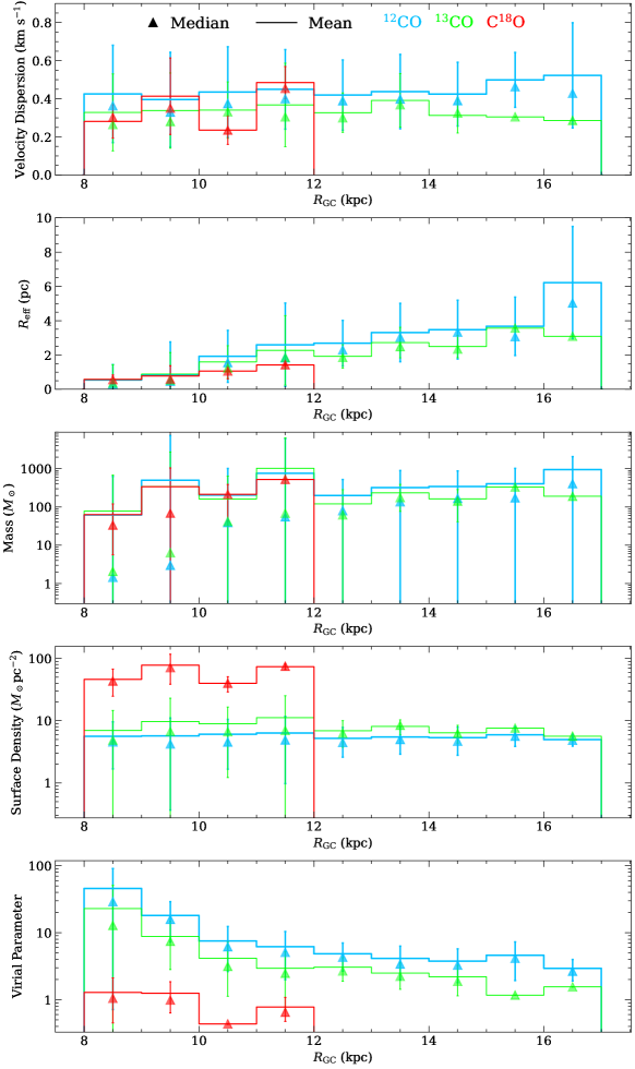
Figure D1: Physical properties of the ¹²CO (blue), ¹³CO (green), and C¹⁸O (red) structures as a function of the Galactocentric radius. Histograms and triangles indicate the mean and median values of physical properties in the $R\rm_{GC}$ bins of 1 kpc width, respectively, and vertical lines correspond to the standard deviations around the mean values. From top to bottom: velocity dispersion, effective radius, mass, mass surface density, and virial parameter. Note that the y-axis is logarithmically scaled for the physical properties whose mean or median values span more than $\sim$2 orders of magnitude along $R\rm_{GC}$.

The physical properties of the ¹²CO, ¹³CO, and C¹⁸O structures within the three spiral arms are presented and compared in this section, including the velocity dispersion ($\sigma_{v}$), effective radius ($R\rm_{eff}$), mass ($M$), mass surface density ($\Sigma$), and virial parameter ($\alpha\rm_{vir}$). Please refer to Appendix C for their definitions. Figure 6 exhibits the histograms of their distributions. The numbers of structures are labeled in the top panels. The median values for each property are also labeled in each panel. Note that the scale range of the x-axis is fixed for each property of the ¹²CO and ¹³CO structures due to their similar dynamic ranges, while it is wider than that for the C¹⁸O structures. Generally speaking, the outskirts of an individual MC are traced by ¹²CO, the moderately dense structures are traced by ¹³CO, and the most dense structures are traced by C¹⁸O. At our current sensitivities, the vast majority of the ¹²CO clouds do not harbor ¹³CO and C¹⁸O structures. And most of the ¹³CO structures do not harbor C¹⁸O structures either (see Section 3.3.3 for details). Therefore, the physical properties derived by the three isotopologs may have different distributions. Besides, plots of the mean and median values of the physical properties at different Galactocentric radii are displayed in Figure D1 in Appendix D.

The velocity dispersions in Figure 6 show narrow distributions that span over $\sim$0.1–2.2$~{}\rm km\,s^{-1}$, $\sim$0.1–2.0$~{}\rm km\,s^{-1}$, and $\sim$0.1–0.9$~{}\rm km\,s^{-1}$ for the ¹²CO, ¹³CO, and C¹⁸O structures, respectively. For each individual CO isotopolog, the median values of $\sigma_{v}$ appear to be the same across the Galactic disk (around $\sim$0.4, 0.3, and 0.3$~{}\rm km\,s^{-1}$ for the ¹²CO, ¹³CO, and C¹⁸O structures, respectively). For the ¹²CO structures, the median value of $\sigma_{v}$ is much lower than those shown by the data from the CfA survey (e.g., $\sim$ 2.8 $\rm km\,s^{-1}$; Miville-Deschênes et al. 2017) and from the MWISP survey with different decomposition algorithms (e.g., $\sim$ 1.1 $\rm km\,s^{-1}$; Ma et al. 2021). However, it is similar to those shown by Sun et al. (2021) from their results for the MWISP data with the same DBSCAN cloud decomposition method. Note that the velocity resolution of the data, the cloud decomposition algorithm, and the local environment of the interstellar medium may all affect the statistics of $\sigma_{v}$.

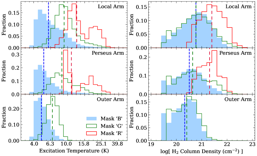
Figure 5: Histograms of the excitation temperatures (left) and H₂ column densities (right). Top to bottom: histograms of the Local, Perseus, and the Outer arms. The mask “B,” “G,” and “R” regions are colored in blue, green, and red, respectively. The vertical dashed lines in the corresponding colors indicate the median values.

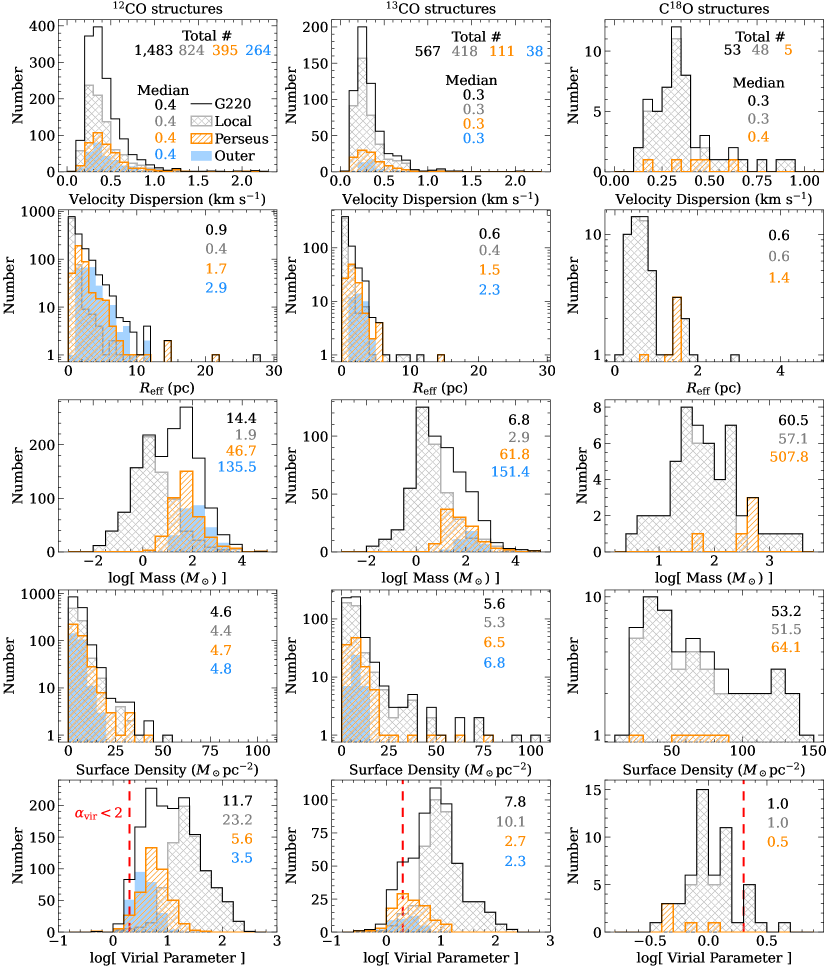
Figure 6: Histograms of the derived physical properties of the ¹²CO (left), ¹³CO (center) and C¹⁸O (right) structures. Distributions for the structures in the whole G220 region and the Local, Perseus, and Outer arms are shown in black, gray, orange, and blue histograms, respectively. Top to bottom: histograms of the velocity dispersion, effective radius, mass, mass surface density, and virial parameter. The median values are labeled in each panel. The total numbers of molecular structures included in the statistics are marked in the top panels. The vertical dashed lines in the bottom panels denote the loci of $\alpha\rm_{vir}=2$.

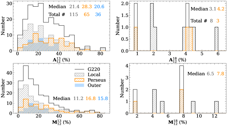
Figure 7: Histograms of $\mathbf{A}^{13}_{12}$ (top-left), $\mathbf{A}^{18}_{12}$ (top-right), $\mathbf{M}^{13}_{12}$ (bottom-left), and $\mathbf{M}^{18}_{12}$ (bottom-right) of MCs in the whole G220 region (black) and the Local (gray), Perseus (orange), and Outer (blue) arms. Please refer to Section 3.3.3 for the definitions of the area and mass ratios. The total numbers of structures included in the statistics and the median values for the ratios are marked.

The cloud sizes and masses of our sample span about 2 and 6 orders of magnitude, respectively. As expected, the dynamic ranges of $R\rm_{eff}$ and $M$, visible in Figure 6, show the highest, medium, and lowest values for the ¹²CO, ¹³CO, and C¹⁸O structures, respectively. Due to the improved sensitivity and resolution of the MWISP data, we detect a large number of small and/or faint structures with subparsec radii and subsolar masses that were largely missed or identified as parts of the large MCs in previous studies. The relatively small and/or faint ¹²CO and ¹³CO structures typically do not contain C¹⁸O structures, possibly due to the C¹⁸O structures suffering more severe beam dilution effects. When compared to the median values that are based on the CfA data within the G220 region, such as Miville-Deschênes et al. (2017, $\sim$17 pc and $\sim$$5\times 10^{3}~{}M_{\odot}$) and Rice et al. (2016, $\sim$17 pc and $\sim$$8\times 10^{3}~{}M_{\odot}$), our ¹²CO samples show the much smaller median values for both $R\rm_{eff}$ and $M$. However, our ¹²CO samples again show similar median $R\rm_{eff}$ and $M$ values to those of Sun et al. (2021, see Tables 6 and 7 therein).

In the entire G220 region, the total masses of the ¹²CO, ¹³CO, and C¹⁸O structures are $4.0\times 10^{5}$, $1.4\times 10^{5}$, and $1.2\times 10^{4}~{}M_{\odot}$, respectively (listed in Column 13 of Table 5). The Local, Perseus, and Outer arms account for $\sim$$38\%$, $\sim$$41\%$, and $\sim$$21\%$ of the total ¹²CO-traced mass in the G220 region, respectively. It seems that the two nearby spiral arms contribute a similar portion of the total molecular gas mass and are more prominent than the Outer arm. Nevertheless, the Perseus arm is much more prominent than the other arms in the G130 region (Sun et al., 2020), with the Local, Perseus, and Outer arms accounting for $\sim$20%, $\sim$70%, and $\sim$10% of the total ¹²CO-traced mass, respectively. Besides, both our ¹²CO- and ¹³CO-traced masses in the Outer arm are two times larger than those of the G130 region. These trends follow the scenario traced by the young stellar population (Carraro et al., 2005; Moitinho et al., 2006; Vázquez et al., 2008) and H I gas (Koo et al., 2017)—the Perseus arm becomes less prominent, while the Outer arm seems to grow, not lessen, from the SGQ to the TGQ.

The mass surface densities of the structures traced by different CO isotopologs vary greatly—by $\sim$2 orders of magnitude. As expected, the ¹²CO structures tracing the relatively diffuse portion of the MCs have the smallest median values of $\Sigma$, while the C¹⁸O structures tracing the relatively dense portion of the MCs have the largest median values of $\Sigma$. For each individual CO isotopolog, the median values of $\Sigma$ are almost constant across different Galactocentric radii (around $\sim$4.6, 5.6, and 53.2$~{}M_{\odot}\,\rm pc^{-2}$ for ¹²CO, ¹³CO, and C¹⁸O structures, respectively). The nearly constant median value of $\Sigma\approx 5~{}M_{\odot}\,\rm pc^{-2}$ for ¹²CO clouds at $R_{\rm GC}\gtrsim 10\rm~{}kpc$ is also reported in previous studies (e.g., Miville-Deschênes et al., 2017; Sun et al., 2021).

Figure 8: Relations between physical properties of the molecular structures traced by different CO isotopologs. Top row: most ¹²CO structures are plotted as small dots; those containing ¹³CO structures are plotted as bigger dots in darker colors; and those further containing C¹⁸O structures are enclosed in black squares. Middle row: similar to the top panels, but for ¹³CO structures. Bottom row: for C¹⁸O structures. Left column: mass vs. effective radius diagram. The yellow shadings, $M(r)\leqslant 870\,M_{\odot}\left(R/\rm pc\right)^{1.33}$, highlight the regions where the clouds fail to form high-mass stars (Kauffmann et al., 2010a, b, 2013; Kauffmann & Pillai, 2010). The solid red lines are the empirical lower limit of the surface density required for massive star formation ($\Sigma=0.05~{}\rm g\,cm^{-2}$, Urquhart et al., 2013a, b). Middle column: velocity dispersion vs. effective radius plot. The first Larson relation revealed by the data from Solomon et al. (1987) is also drawn with the cyan line for comparison. Right column: virial parameter as a function of mass. The pink shadings indicate the regions of $\alpha\rm_{vir}<2$. The black solid, black dashed, and green solid lines delineate the log–log linear least-squares fitting relations between the physical properties of the ¹²CO, ¹³CO, and C¹⁸O structures, respectively. The fitting results are also annotated in each graph, with the Pearson correlation coefficients marked in parentheses.

The virial parameter describes the balance between the kinetic and gravitational energies of the MCs. The vertical dashed lines in the last row of Figure 6 demarcate the gravitationally bound structures ($\alpha\rm_{vir}<2$) from the unbound structures ($\alpha\rm_{vir}\geqslant 2$; Kauffmann et al. 2013). We find that only a very small fraction of ¹²CO structures appear to be bound, with the percentages of $\sim$$0.5\%$, $\sim$$4.1\%$, and $\sim$$8.0\%$ for the Local, Perseus, and Outer arms, respectively. And there are $\sim$$3.1\%$, $\sim$$32.4\%$, and $\sim$$42.1\%$ gravitationally bound ¹³CO structures in the Local, Perseus, and Outer arms, respectively. Unlike the ¹²CO and ¹³CO structures, the C¹⁸O structures are more likely to be bound, i.e., $\sim$$86.8\%$ of the C¹⁸O structures in the entire G220 region have $\alpha\rm_{vir}<$2. In addition, the median $\alpha\rm_{vir}$ values in the Perseus and Outer arms are much lower than those in the Local arm. This seems to be a consequence of the increasing detection limit. In the more distant arms, we miss smaller structures that tend to have relatively high $\alpha\rm_{vir}$ values (as shown in Section 3.4).

3.3.3 Dense Gas Fraction

In the entire G220 region, there are 216 ¹²CO clouds ($\sim$15%) containing ¹³CO dense structures and 11 ¹²CO clouds ($\sim$0.7%) containing C¹⁸O dense structures. The proportion of $\sim$15% is consistent with that measured by the MWISP survey in the SGQ (Yuan et al., 2022). Besides, the proportions for ¹²CO clouds harboring ¹³CO dense structures are similar across the Galactic disk, with $\sim$14%, $\sim$16%, and $\sim$14% in the Local, Perseus, and Outer arms, respectively. One can see that typically only a small fraction of ¹²CO clouds harbor ¹³CO and/or C¹⁸O dense structures. To understand the contributions of the dense structures to the MCs, we define the area ratios as follows: $\mathbf{A}^{13}_{12}\equiv A\left({\rm{}^{13}CO}\right)/A\left({\rm{}^{12}CO}\right)$ and $\mathbf{A}^{18}_{12}\equiv A\left({\rm C^{18}O}\right)/A\left({\rm{}^{12}CO}\right)$ where $A\left(\rm{}^{12}CO\right)$, $A\left(\rm{}^{13}CO\right)$, and $A\left(\rm C^{18}O\right)$ are the area of the ¹²CO cloud and the total areas of the ¹³CO and C¹⁸O dense structures within each ¹²CO cloud, respectively. Similarly, we define the mass ratios as $\mathbf{M}^{13}_{12}\equiv M\left({\rm{}^{13}CO}\right)/M\left({\rm{}^{12}CO}\right)$ and $\mathbf{M}^{18}_{12}\equiv M\left({\rm C^{18}O}\right)/M\left({\rm{}^{12}CO}\right)$ where $M\left(\rm{}^{12}CO\right)$, $M\left(\rm{}^{13}CO\right)$, and $M\left(\rm C^{18}O\right)$ are the mass of the ¹²CO cloud and the total masses of the ¹³CO and C¹⁸O dense structures within each ¹²CO cloud, respectively.

The histograms of the ratios are plotted in Figure 7. The area ratios $\mathbf{A}^{13}_{12}$ and $\mathbf{A}^{18}_{12}$ span ranges from $\sim$1.2% to 80% and from $\sim$0.9% to 5.9%, respectively. The distributions of the mass ratios are similar to the area ratios, ranging from $\sim$0.3% to 76.6% and from $\sim$1.6% to 12.3% for $\mathbf{M}^{13}_{12}$ and $\mathbf{M}^{18}_{12}$, respectively. Yuan et al. (2022) reported a sharp upper limit of $\mathbf{A}^{13}_{12}=70\%$, and it is notable that, in general, our $\mathbf{A}^{13}_{12}$ values are indeed below this upper limit. Moreover, we see that the median values (labeled in each panel) of $\mathbf{A}^{18}_{12}$ and $\mathbf{M}^{18}_{12}$ are quite small, suggesting that the C¹⁸O dense structures typically occupy only a very small fraction of areas and masses in MCs.

3.4 Relations between Physical Properties

Figure 8 shows the relations between the physical properties of the ¹²CO (top panels), ¹³CO (center panels), and C¹⁸O (bottom panels) structures. One can see that the ¹²CO clouds that contain ¹³CO and/or C¹⁸O dense structures and the ¹³CO structures that contain C¹⁸O dense structures generally have the largest sizes and masses and the most turbulent velocity dispersions. The log–log linear least-squares fitting results are labeled in the diagrams, with the Pearson correlation coefficients marked in parentheses.

A power-law relation between mass and radius, $M\propto R^{2}$, is available from Larson (1981), indicating the clouds having a nearly constant surface density. Kauffmann et al. (2010a, b) treated the exponent of the $M$–$R$ relation as a proxy for how column density varies with radius. The left panels of Figure 8 show the strong correlations (Pearson correlation coefficients $r\gtrsim 0.95$) between $\log(M)$ and $\log(R\rm_{eff})$ for the ¹²CO, ¹³CO, and C¹⁸O structures, with the exponents $\beta=2.15$, 2.35, and 2.34, respectively. We find that the $\beta$ values fitted from the ¹³CO, and C¹⁸O structures are very close to those measured by the Galactic Ring Survey (GRS) survey (Roman-Duval et al., 2010), while those fitted from the ¹²CO structures are closer to Larson’s results.

Table 6: Basic Properties of Peculiar MCs

Name		$v\rm_{\scriptscriptstyle LSR}$	$\sigma_{v}$									Dist.	$R\rm_{eff}$	Mass		$\alpha\rm_{vir}$	$\mathbf{A}^{13}_{12}$	$\mathbf{M}^{13}_{12}$	$\mathbf{A}^{18}_{12}$	$\mathbf{M}^{18}_{12}$	Arm
		($\rm km\,s^{-1}$)	($\rm km\,s^{-1}$)									(kpc)	(pc)	($M_{\odot}$)			(%)	(%)	(%)	(%)
MWISP G220.634$-$1.916		11.7	2.22									1.0	9.7	$8.3\times 10^{3}$		6.7	52.8	42.7	1.8	4.0	Local
MWISP G221.775$-$3.007		12.9	1.05									1.0	11.3	$1.0\times 10^{4}$		1.4	44.5	37.7	0.9	1.6	Local
MWISP G224.440$-$1.069		16.3	1.91									1.1	27.9	$1.0\times 10^{5}$		1.1	50.5	52.7	3.9	9.1	Local
MWISP G221.921$-$2.121		39.3	1.19									3.7	21.4	$6.5\times 10^{4}$		0.5	58.6	67.3	0.9	1.6	Perseus
MWISP G223.736$-$2.027		63.0	0.88									6.6	11.2	$4.7\times 10^{3}$		2.2	22.3	18.8	$\cdots$	$\cdots$	Outer

The $M$–$R$ diagrams can also be used to investigate the possible high-mass star forming sites. The yellow shadings in Figure 8 represent the region where clouds are not massive enough to form high-mass stars, i.e., $M(r)\leqslant 870\,M_{\odot}\left(R/\rm pc\right)^{1.33}$ (Kauffmann et al., 2010a, b, 2013; Kauffmann & Pillai, 2010). The solid red lines trace the empirical minimum threshold required for massive star formation—surface density equal to $0.05~{}\rm g\,cm^{-2}$ (Urquhart et al., 2013a, b). We find that none of our structures reaches the threshold of Urquhart et al. (2013a, b), and only two ¹²CO clouds (MWISP G224.440$-$1.069 and MWISP G221.921$-$2.121; see Figure 9) together with two ¹³CO structures (MWISP G223.939$-$1.895 and MWISP G221.954$-$2.090) lie above the border of Kauffmann et al. (2010a, b, 2013) and Kauffmann & Pillai (2010). We also find that the two ¹³CO structures match the two ¹²CO clouds, respectively, which are the most massive MCs ($\gtrsim$$6\times 10^{4}~{}M_{\odot}$) in the G220 region. The scarcity of high-mass star formation is consistent with the literature, i.e., no 6.7 GHz methanol maser has been detected in the G220 region (according to the MaserDB database; Ladeyschikov et al., 2019).

The velocity dispersion–size relation of the form $\sigma_{v}\propto R^{0.5}$ is well known as the first Larson relation (the cyan line in Figure 8; Larson, 1981; Solomon et al., 1987; Heyer & Brunt, 2004). The middle panels of Figure 8 render the moderate correlations between $\log(\sigma_{v})$ and $\log(R\rm_{eff})$ with the Pearson correlation coefficients $r=0.44$, 0.54, and 0.67 for the ¹²CO, ¹³CO, and C¹⁸O structures, respectively. We find that the exponents traced by the ¹²CO and ¹³CO structures in the TGQ ($\beta=0.17$ and 0.25, respectively) are comparable with those observed by the MWISP survey in the SGQ (Li et al., 2020; Ma et al., 2021). However, these $\beta$ values are much shallower than the Larson relation. The shallow $\sigma_{v}$–$R\rm_{eff}$ relations may be due to the fact that the small clouds deviates from the Larson relation. Similar to Benedettini et al. (2020), we again perform least-squares fits to the ¹²CO clouds at two different scales. For those with radius $R_{\rm eff}\geqslant 2\rm~{}pc$, the best fit gives $\beta=0.55$ (and $r=0.55$), which is in good agreement with the Larson relation, whereas the best fit for those with $R_{\rm eff}<2\rm~{}pc$ is flatter ($\beta=0.11$ and $r=0.25$), which deviates significantly from the Larson relation. These are basically consistent with the results of Benedettini et al. (2020).

Figure 9: Integrated intensity maps and spectra of the MCs MWISP G220.634$-$1.916, G221.775$-$3.007, G224.440$-$1.069, G223.736$-$2.027, and G221.921$-$2.121. The ¹²CO, ¹³CO, and C¹⁸O lines are drawn in blue, green, and red, respectively. The integrated intensity maps are shown in a square-root scale to clearly visualize the faint parts of the MCs, and the color bars represent integrated intensity in units of $\rm K~{}km\,s^{-1}$. The spectra shown in each plot, with the y-axis on the $T_{\rm MB}$ scale, are averaged over a $90\arcsec\times 90\arcsec$ ($3\times 3$ pixels) region selected around the brightest pixel of each MC. The magenta crosses denote the 22 GHz H₂O masers detected toward the star formation regions (Han et al., 1998; Valdettaro et al., 2001; Sunada et al., 2007; Urquhart et al., 2011). The H II regions from Blitz et al. (1982) and the WISE catalog (Anderson et al., 2014) are marked as green and yellow circles, respectively.

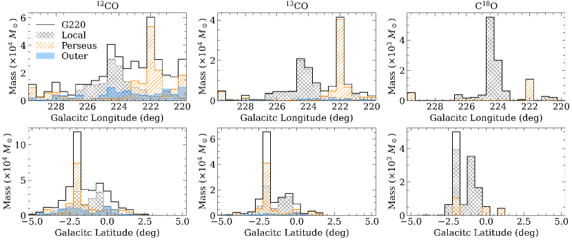
Figure 10: Molecular gas distributions along the Galactic longitude (upper panels) and the Galactic latitude (lower panels), integrated over a Galactic latitude range from $-5\fdg 25$ to $5\fdg 25$ and a Galactic longitude range from $219\fdg 75$ to $229\fdg 75$, respectively. The mass distributions of the whole G220 region and the Local, Perseus, and Outer arms are shown in black, gray, orange, and blue histograms, respectively. And the mass distributions traced by ¹²CO, ¹³CO, and C¹⁸O are exhibited in the left, middle, and right panels, respectively.

For pressure-confined objects (i.e., $\alpha\rm_{vir}\gg 1$), Bertoldi & McKee (1992) predicted a theoretical power-law correlation between virial parameters and masses with an exponent equal to $-\text@frac{2}{3}$. In Figure 8 (right panels), anticorrelations over a broad mass range can be seen. We notice that the correlations for the ¹²CO and ¹³CO structures are well defined ($r\sim-0.8$), while the correlation for C¹⁸O structures is just modest ($r=-0.39$). The exponents for ¹²CO and ¹³CO structures ($=-0.36$ and $-0.35$, respectively) are similar to that reported by Kauffmann et al. (2013) from their analysis of the GRS data (Roman-Duval et al., 2010). These anticorrelation trends reflect a scenario in which more massive clouds are more gravitationally bound and therefore less stable—more likely to collapse without the additional support, such as from a strong magnetic field (Kauffmann et al., 2013). Moreover, the masses in the bound ¹²CO, ¹³CO, and C¹⁸O structures account for $\sim$54.1%, $\sim$82.4%, and $\sim$96.8% of the total ¹²CO, ¹³CO, and C¹⁸O masses, respectively. These mass proportions for the bound structures are much higher than the number proportions (see Section 3.3.2). We can then conclude that, despite their small numbers, gravitationally bound molecular structures hold most of the molecular masses.

3.5 Massive MCs Presentation

The high-sensitivity and high-resolution MWISP ¹²CO, ¹³CO, and C¹⁸O data provide an excellent opportunity to observe the elaborate morphologies of the MCs. In this section, we present five peculiar MCs that show filamentary structures and represent the most massive MCs in the three spiral arms. Their basic properties are tabulated in Table 6. Interestingly, the dense gas fractions in these clouds are generally higher than the typical values marked in Figure 7 for each arm component. Their integrated intensity maps and spectra are shown in Figure 9, with ¹²CO, ¹³CO, and C¹⁸O drawn in blue, green, and red, respectively. In each image, we also mark the associated 22 GHz H₂O maser sources, by using the MaserDB database (Ladeyschikov et al., 2019), and the associated H II regions, by referring to Blitz et al. (1982) and the Wide-Field Infrared Survey Explorer (WISE) catalog of Galactic H II regions v2.2 (Anderson et al., 2014, hereafter, the WISE catalog). The following descriptions of the MCs are in the order of the maps in Figure 9.

MWISP G220.634$-$1.916. This cloud has the largest velocity dispersion ($\sim$$2.2\rm~{}km\,s^{-1}$) in the G220 region. The optically thick ¹²CO spectral line around the emission peak exhibits an obvious red asymmetric structure. We find a that 22 GHz H₂O maser (Han et al., 1998) and two H II regions (Blitz et al., 1982) are associated with this cloud.

MWISP G221.775$-$3.007. The optically thick ¹²CO molecular line around the emission peak shows a significant red asymmetric structure.

MWISP G224.440$-$1.069. This cloud is the most massive MC, accounting for $\sim$26%, $\sim$38%, and $\sim$76% of the total ¹²CO, ¹³CO, and C¹⁸O traced masses in the entire G220 region, respectively. It traces the CMa OB1 complex, which has been studied in detail by the previous works, such as Kim et al. (2004), Elia et al. (2013), and Lin et al. (2021). A total of seven 22 GHz H₂O masers (e.g., Sunada et al., 2007; Urquhart et al., 2011) and three H II regions (according to the WISE catalog) are associated with this cloud.

MWISP G223.736$-$2.027. It does not contain any C¹⁸O dense structures. This source shows the typical filamentary structure even at a distance of $\sim$6.6 kpc. None of the known 22 GHz H₂O masers and H II regions are associated with this cloud.

MWISP G221.921$-$2.121. This is the second most massive MC in the G220 region. A 22 GHz H₂O maser has been detected toward it (e.g., Valdettaro et al., 2001). Two H II regions from the WISE catalog and one H II region from Blitz et al. (1982) are associated with this cloud.

Figure 11: Left: locations of the MCs projected on the Galactic plane. The plan view of the Milky Way (Reid et al., 2019) is overlaid. The straight dashed lines denote the directions of the Galactic longitude $l=180\degree$, $210\degree$, $240\degree$, and $270\degree$. The Sun (red Sun symbol) is at (0, 8.15) kpc. The solid gray, orange, and blue curved lines trace the centers (and the dotted curved lines indicate the widths enclosing $90\%$ of the high-mass star-forming regions of Reid et al. 2019) of the Local, Perseus, and Outer arms, respectively. Right: distribution of the $\it z$-scale height vs. the Galactocentric radius $R\rm_{GC}$. The Galactic plane ($z=0$) is drawn with the dashed line. The Sun (red Sun symbol) is at ($8.15\rm~{}kpc$, $5.5\rm~{}pc$). The red crosses indicate the centers of $R\rm_{GC}$ and $\it z$ of the three arms, whose values are also marked. The red bars denote the thicknesses of the arms, with their values noted on the side. In both panels, the lightest, medium, and darkest filled circles represent the ¹²CO, ¹³CO, and C¹⁸O structures, respectively. The symbol size is proportional to $\log\left(M\right)$. The proportions of the three CO isotopologs are different for the convenience of presentation.

4 3D Distributions in the Milky Way

In order to understand the mass distributions, we calculate the total molecular mass within every $0.5\degree$ of the Galactic longitude and latitude, respectively. The mass distributions along the $l$ (upper panels) and $b$ (lower panels) directions are depicted in Figure 10, with those traced by ¹²CO, ¹³CO, and C¹⁸O plotted in the left, center, and right panels, respectively.

We notice that in each individual spiral arm, the distribution peaks of the masses traced by ¹²CO, ¹³CO, and C¹⁸O are approximately at the same $l$ and $b$. Along the $l$ direction, most of the molecular masses are distributed in the range of $l<225\degree$. The mass distributions in the Local arm are concentrated at $l\sim 224\degree$, while those in the Perseus arm are concentrated at $l\sim 222\degree$. And there is no significant mass peak along the $l$ direction in the Outer arm. This suggests that the molecular gas is unevenly distributed along the Local and Perseus arms, but appears to be more evenly distributed along the Outer arm. After close examination, we find that the distribution peaks of the Local and Perseus arms correspond to the aforementioned massive MCs MWISP G224.440$-$1.069 and MWISP G221.921$-$2.121 (Figure 9), respectively. Along the $b$ direction, the majority of the molecular gases are distributed in the range of $b<0\degree$. According to the ¹³CO maps of Kim et al. (2004), the Local arm in the G220 region extends to at least $b\sim-10\degree$, therefore it is important to note that our data do not actually cover the entire Local arm (also mentioned in Section 3.1). However, the Perseus and Outer arms seem to be almost completely mapped. The masses of the Perseus arm are concentrated at $b\sim-2\degree$. The Outer arm has no significant distribution peak along the $b$ direction either.

The face-on and vertical distributions of the MCs are displayed in Figure 11, with the circle sizes proportional to $\log\left(M\right)$. In both maps, the Outer arm traced by the molecular gas appears prominently in this Galactic range for the first time, although it has been well described by other spiral arm tracers (Carraro et al., 2005; Moitinho et al., 2006; Vázquez et al., 2008; Koo et al., 2017). Furthermore, we find that the spiral arms traced by MCs are different from the arm model of Reid et al. (2019) in the face-on map. The discrepancy may be attributed to both the uncertainty of the kinematic distances and the bias of very few maser targets in the arm model. Along the $z$-direction, the MCs seem to be asymmetrically distributed. The minimum $z$ of the MCs reaches $\sim$$-600\rm~{}pc$, while the maximum $z$ only reaches $\sim$$400\rm~{}pc$. A substantial proportion ($\sim$$75\%$) of the molecular structures fall below the Galactic plane. In addition, we see that the dynamic ranges of the MCs’ $z$-scale heights are increasing with the Galactocentric radius $R_{\rm GC}$. These reveal evident pictures of the Galactic disk warping and flaring (Burke, 1957; Kerr, 1957; Westerhout, 1957; Burton, 1988; Wouterloot et al., 1990) in the G220 region.

To better quantify the warp and flare of the molecular gas disk, we derive the arm ($R_{\rm GC}$, $z$) centers by the mass-weighted average of the MCs’ $R_{\rm GC}$ and $z$-scale height, and we derive the arm thicknesses by the mass-weighted standard deviation of the MCs’ $z$-scale height. The center positions are drawn as red crosses, and the thicknesses are marked with red bars in Figure 11. The derived ($R_{\rm GC}$, $z$) centers of the Local, Perseus, and Outer arms are located at about (9, $-$23), (11, $-$90), and (14, $-$162) in units of (kpc, pc), respectively. The thicknesses of the Local, Perseus, and Outer arms are about 48, $201$, and $457$ pc, respectively. The Outer arm is more than twice as thick as the Perseus arm. Obviously, both the vertical displacements and thicknesses of the spiral arms are increasing with $R_{\rm GC}$. These results are consistent with those traced by other spiral arm tracers in the same Galactic longitude range, such as H I and stellar emission (e.g., Gum et al., 1960; Russeil, 2003).

5 Summary

Using the high-quality MWISP data, we conducted a large-scale ¹²CO, ¹³CO, and C¹⁸O ($J=1$–0) survey in the G220 region, i.e., $l=[\,219\fdg 75,~{}229\fdg 75\,]$ and $b=[\,-5\fdg 25,~{}5\fdg 25\,]$ (105 deg² in total), and obtained 1,514,461 spectra for each CO isotopolog. According to the $l$–$v$ maps, the entire G220 region is divided into the Local, Perseus, and Outer arms that are discussed. Our main results can be summarized as follows.

1. We identified a total of 1,502 ¹²CO, 570 ¹³CO, and 53 C¹⁸O molecular structures by using the DBSCAN algorithm. There are 216 ¹²CO structures containing ¹³CO dense structures and 11 ¹²CO structures containing C¹⁸O dense structures.

2. The G220 region is generally in the low-excitation and low-density phase. The total masses of the ¹²CO, ¹³CO, and C¹⁸O structures are estimated to be $4.0\times 10^{5}$, $1.4\times 10^{5}$, and $1.2\times 10^{4}~{}M_{\odot}$, respectively. The Local, Perseus, and Outer arms account for $\sim$$38\%$, $\sim$$41\%$, and $\sim$$21\%$ of the total ¹²CO-traced mass in the G220 region, respectively. Comparing to the SGQ (Sun et al., 2020), we notice that in the TGQ, the Outer arm appears to be more conspicuous, while the Perseus arm is less prominent.

3. Our survey resolves the molecular structures at different scales, i.e., with the effective radii of $\sim$0.04–$27.9\rm~{}pc$ and masses of $\sim$$10^{-2}$–$10^{5}~{}M_{\odot}$. The vast majority of the ¹²CO and ¹³CO structures appear to be gravitationally unbound ($\alpha\rm_{vir}\geqslant 2$), while the C¹⁸O structures are more likely to be bound ($\alpha\rm_{vir}<2$).

4. Strong $M$–$R\rm_{eff}$ correlations and tight $\alpha\rm_{vir}$–$M$ anticorrelations are observable. However, the correlations between $\sigma_{v}$ and $R\rm_{eff}$ appear to be not obvious over the full dynamic range.

5. For the Local, Perseus, and Outer arms, the derived arm $(R_{\rm GC},~{}z)$ centers are about (9, $-$23), (11, $-$90), and (14, $-$162) in units of (kpc, pc), and the derived arm thicknesses are about 48, $201$, and $457\rm~{}pc$, respectively. Both the vertical displacements and thicknesses of the spiral arms are increasing with the Galactocentric radius.

Table B1: Physical Properties of Molecular Structures

Index	Name	$v\rm_{\scriptscriptstyle LSR}$	$\sigma_{v}$					$W\rm_{CO}$	$T_{\rm peak}$	Dist.	$R\rm_{eff}$	Area	Mass	$\Sigma$	$M_{\rm vir}$	$\alpha\rm_{vir}$	Arm	Flag	Matching
		($\rm km\,s^{-1}$)	($\rm km\,s^{-1}$)					($\rm K~{}km\,s^{-1}$)	(K)	(kpc)	(pc)	(pc2)	($M_{\odot}$)	($M_{\odot}\rm~{}pc^{-2}$)	($M_{\odot}$)				12CO cloud
4	MWISP G220.634$-$1.916	11.66	2.22					6.4	27.5	1.00		294.8	$8.3\times 10^{3}$	28.1	$5.6\times 10^{4}$	6.7	Loc	12	$\cdots$
892	MWISP G222.927$+$0.922	31.31	0.31					2.3	9.2	2.84		8.9	$8.7\times 10^{1}$	9.8	$1.8\times 10^{2}$	2.1	Per	12	$\cdots$
1282	MWISP G223.302$-$0.333	53.71	0.40					2.1	5.8	5.33		60.7	$5.6\times 10^{2}$	9.2	$8.0\times 10^{2}$	1.4	Out	12	$\cdots$
1640	MWISP G220.312$-$1.740	13.80	0.53					1.1	3.6	1.00		6.2	$8.8\times 10^{1}$	14.2	$4.7\times 10^{2}$	5.3	Loc	13	4
1975	MWISP G221.954$-$2.090	39.59	0.87					2.8	9.1	3.73		661.7	$4.1\times 10^{4}$	61.2	$1.3\times 10^{4}$	0.3	Per	13	953
2061	MWISP G227.939$-$0.138	66.08	0.36					0.6	1.4	6.59		19.3	$1.6\times 10^{2}$	8.4	$3.5\times 10^{2}$	2.1	Out	13	1421
2068	MWISP G229.744$+$0.117	70.29	0.33					0.6	1.8	6.99		30.0	$2.7\times 10^{2}$	9.1	$3.7\times 10^{2}$	1.4	Out	13	1468
2077	MWISP G220.677$-$1.866	12.28	0.40					0.5	2.2	1.00		1.9	$1.2\times 10^{2}$	65.0	$1.4\times 10^{2}$	1.1	Loc	18	4
2125	MWISP G229.578$+$0.153	52.90	0.60					0.5	1.1	4.92		8.2	$5.3\times 10^{2}$	64.1	$6.3\times 10^{2}$	1.2	Per	18	1204

Note. — Column (1): index of the source. Column (2): source name given by the MWISP project and the Galactic coordinates of the cloud centroid. Columns (3)–(4): LSR velocity and velocity dispersion. Column (5): average integrated intensity across the area of the structure. Column (6): peak main-beam temperature. Columns (7)–(13): heliocentric distance, effective radius, area, mass, mass surface density, virial mass, and virial parameter. Column (14): spiral arm layer. Column (15): flag—“12”, “13”, and “18” denote samples traced (and their physical properties estimated) by the ¹²CO, ¹³CO, and C¹⁸O lines, respectively. Column (16): index of the matching ¹²CO cloud for the ¹³CO and C¹⁸O structures. Only a small portion of the catalog is shown here, and a machine-readable version of the full table is published at Science Data Bank: https://doi.org/10.57760/sciencedb.07765 (Dong et al., 2023).

Appendix A Data with the bad channels

The $l$–$v$ map of the “uncleaned” ¹²CO emission is shown in Figure A1. The integration ranges are $-5\fdg 25\leqslant b\leqslant 5\fdg 25$. The map includes the spurious signals caused by $\sim$$34~{}\rm km\,s^{-1}$ bad channels.

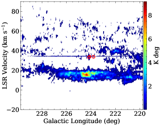
Figure A1: Longitude–velocity map of the “uncleaned” ¹²CO emission, integrated over a Galactic latitude range from $-5\fdg 25$ to $5\fdg 25$. The three MCs in red circles are contaminated by the bad channels.

Appendix B Properties of Molecular Structures

The physical properties of the ¹²CO, ¹³CO, and C¹⁸O molecular structures are summarized in Table B1.

Appendix C Derivation of Physical Properties

This appendix presents the equations used to estimate the physical properties.

C.1 Excitation Temperature

Assuming that the ¹²CO line is optically thick and that the beam-filling factors are near unity, the excitation temperature in each pixel of the MC can be expressed as (e.g., Bourke et al., 1997)

$$T_{\rm ex}=\frac{5.532}{\ln\left[\,1+5.532/\left(T\rm_{MB,pk}\!\left({}^{12}CO\right)+0.819\right)\,\right]},$$ (C1)

where $T{\rm{}_{MB,pk}\!\left({}^{12}CO\right)}$ is the peak main-beam brightness temperature of ¹²CO.

C.2 $\rm H_{2}$ Column Density

The H₂ column density for the ¹²CO clouds can be estimated by simply multiplying the integrated intensities of ¹²CO ($\int T{\rm{}_{MB}\!\left({}^{12}CO\right)}\,dv$) by the commonly used CO-to-H₂ conversion factor $X_{\rm CO}=2.0\times 10^{20}~{}\rm cm^{-2}\left(K~{}km/s\right)^{-1}$ (Bolatto et al., 2013). For the ¹³CO and C¹⁸O structures, the H₂ column density can be derived using the LTE method, which is based on the assumption of the equal excitation temperatures for ¹²CO, ¹³CO, and C¹⁸O in the LTE conditions.

Firstly, the optical depths of the ¹³CO and C¹⁸O lines in each pixel of the molecular structure are given by

$$\tau\!\left(\rm{}^{13}CO\right)=-\ln\! \left[1-\frac{T{\rm{}_{MB,pk}\!\left({}^{13}CO\right)}}{5.29}\right.$$

$$\left.\times\left(\frac{1}{e^{5.29/T_{\rm ex}}-1}-0.164\right)^{-1}\right]$$ (C2)

and

$$\tau\!\left(\rm C^{18}O\right)=-\ln\! \left[1-\frac{T{\rm{}_{MB,pk}\!\left(C^{18}O\right)}}{5.27}\right.$$

$$\left.\times\left(\frac{1}{e^{5.27/T_{\rm ex}}-1}-0.166\right)^{-1}\right],$$ (C3)

where $T\rm_{MB,pk}\!\left({}^{13}CO\right)$ and $T\rm_{MB,pk}\!\left(C^{18}O\right)$ are the peak main-beam brightness temperatures of ¹³CO and C¹⁸O, respectively. In general, the C¹⁸O line is optically thin. For the ¹³CO line, we find that the median, 5th percentiles, and 95th percentile values of $\tau\!\left(\rm{}^{13}CO\right)$ are $\sim$0.27, 0.12, and 0.67, respectively. This suggests that the ¹³CO line can be considered optically thin for almost all pixels of our ¹³CO structures. Then, the ¹³CO and C¹⁸O column densities in each pixel of the molecular structure can thus be expressed as (Bourke et al., 1997; Pineda et al., 2010)

$$N_{\rm{}^{13}CO}=2. 42\times{10}^{14}\times\frac{\tau\!\left(\rm{}^{13}CO\right)}{1-e^{-\tau\!\left(\rm{}^{13}CO\right)}}$$

$$\times\frac{1+0.88/T_{\rm ex}}{1-e^{-5.29/T_{\rm ex}}}\int\!T_{\rm MB}\!\left(\rm{}^{13}CO\right)\,dv$$ (C4)

and

$$N_{\rm C^{18}O}=2. 54\times{10}^{14}\times\frac{\tau\!\left(\rm C^{18}O\right)}{1-e^{-\tau\!\left(\rm C^{18}O\right)}}$$

$$\times\frac{1+0.88/T_{\rm ex}}{1-e^{-5.27/T_{\rm ex}}}\int\!T_{\rm MB}\!\left(\rm C^{18}O\right)\,dv.$$ (C5)

Finally, the isotope ratios of $\left[\rm{}^{12}C/^{13}C\right]=6.21\it R\rm_{GC}+18.71$ ($R_{\rm GC}$ is the Galactocentric radius in units of kpc; Milam et al., 2005) and $\left[\rm{}^{16}O/^{18}O\right]=560$ (Wilson & Rood, 1994) and an abundance ratio of $\left[\rm H_{2}/^{12}C\right]=1.1\times 10^{4}$ (Frerking et al., 1982) are adopted to convert the ¹³CO and C¹⁸O column densities to H₂ column densities.

C.3 Mass, Mass Surface Density, Effective Radius, Velocity Dispersion, and Virial Parameter

The mass of the molecular structure is estimated as $M=2\mu m_{\scriptscriptstyle\rm H}a^{2}d^{2}\sum\nolimits_{i}N_{\rm H_{2}}$, where $\mu=1.36$ is the mean atomic weight, taking the contribution of helium and metals into account, $m\rm{}_{H}$ is the mass of a hydrogen atom, $a=30\arcsec$ is the angular size of a pixel, and $d$ is the heliocentric distance.

The mass surface density, in units of $M_{\odot}~{}\rm pc^{-2}$, is simply calculated by $\Sigma=M/\left(A\times d^{2}\right)$, where $A=a^{\rm 2}\times N_{\rm pixel}$ is the angular area (projected area) of the molecular structure.

Assuming that the cloud is spherical, the effective radius can thus be expressed as $R_{\rm eff}=d\,\sqrt{\frac{A}{\pi}-\frac{\theta^{2}_{\rm MB}}{4}}$ (Ladd et al., 1994), where $\theta_{\rm MB}\sim 50\arcsec$ is the beam size.

The velocity dispersion ($\sigma_{v}$) of the molecular structure is defined as the $T\rm_{MB}$-weighted second moment within the PPV voxels of the structure. Then, the line width of the molecular structure is estimated as $\Delta v=\sqrt{8\ln 2}\times\sigma_{v}$.

The virial mass can be calculated by $M_{\rm vir}=210\times R_{\rm eff}\times\left(\Delta v\right)^{2}$ (MacLaren et al., 1988), where $R_{\rm eff}$ is in units of pc, $\Delta v$ is in units of $\rm km\,s^{-1}$, and the derived $M_{\rm vir}$ is in units of $M_{\odot}$. Then, the virial parameter is defined as $\alpha_{\rm vir}=M_{\rm vir}/M$.

Appendix D Physical Properties at different Galactocentric radii

This appendix presents the mean and median values of physical properties as a function of the Galactocentric radius.

References

- Anderson et al. (2014) Anderson, L. D., Bania, T. M., Balser, D. S., et al. 2014, ApJS, 212, 1, doi: 10.1088/0067-0049/212/1/1
- Astropy Collaboration et al. (2013) Astropy Collaboration, Robitaille, T. P., Tollerud, E. J., et al. 2013, A&A, 558, A33, doi: 10.1051/0004-6361/201322068
- Astropy Collaboration et al. (2018) Astropy Collaboration, Price-Whelan, A. M., Sipőcz, B. M., et al. 2018, AJ, 156, 123, doi: 10.3847/1538-3881/aabc4f
- Barnes et al. (2018) Barnes, P. J., Hernandez, A. K., Muller, E., & Pitts, R. L. 2018, ApJ, 866, 19, doi: 10.3847/1538-4357/aad4ab
- Barnes et al. (2015) Barnes, P. J., Muller, E., Indermuehle, B., et al. 2015, ApJ, 812, 6, doi: 10.1088/0004-637X/812/1/6
- Benedettini et al. (2020) Benedettini, M., Molinari, S., Baldeschi, A., et al. 2020, A&A, 633, A147, doi: 10.1051/0004-6361/201936096
- Benedettini et al. (2021) Benedettini, M., Traficante, A., Olmi, L., et al. 2021, A&A, 654, A144, doi: 10.1051/0004-6361/202141433
- Bertoldi & McKee (1992) Bertoldi, F., & McKee, C. F. 1992, ApJ, 395, 140, doi: 10.1086/171638
- Blitz et al. (1982) Blitz, L., Fich, M., & Stark, A. A. 1982, ApJS, 49, 183, doi: 10.1086/190795
- Bolatto et al. (2013) Bolatto, A. D., Wolfire, M., & Leroy, A. K. 2013, ARA&A, 51, 207, doi: 10.1146/annurev-astro-082812-140944
- Bourke et al. (1997) Bourke, T. L., Garay, G., Lehtinen, K. K., et al. 1997, ApJ, 476, 781, doi: 10.1086/303642
- Brand & Wouterloot (1995) Brand, J., & Wouterloot, J. G. A. 1995, A&A, 303, 851
- Burke (1957) Burke, B. F. 1957, AJ, 62, 90, doi: 10.1086/107463
- Burton (1988) Burton, W. B. 1988, The Structure of Our Galaxy Derived from Observations of Neutral Hydrogen, ed. G. L. Verschuur & K. I. Kellermann (New York, NY: Springer New York), 295–358. https://doi.org/10.1007/978-1-4612-3936-9_7
- Carraro et al. (2005) Carraro, G., Vázquez, R. A., Moitinho, A., & Baume, G. 2005, ApJ, 630, L153, doi: 10.1086/491787
- Choi et al. (2014) Choi, Y. K., Hachisuka, K., Reid, M. J., et al. 2014, ApJ, 790, 99, doi: 10.1088/0004-637X/790/2/99
- Clariá (1974) Clariá, J. J. 1974, A&A, 37, 229
- Dame et al. (2001) Dame, T. M., Hartmann, D., & Thaddeus, P. 2001, ApJ, 547, 792, doi: 10.1086/318388
- Dame et al. (1987) Dame, T. M., Ungerechts, H., Cohen, R. S., et al. 1987, ApJ, 322, 706, doi: 10.1086/165766
- Dong et al. (2023) Dong, Y., Sun, Y., Xu, Y., et al. 2023, Physical properties of molecular structures in the G220 region, V2, Science Data Bank, doi: 10.57760/sciencedb.07765
- Du et al. (2017) Du, X., Xu, Y., Yang, J., & Sun, Y. 2017, ApJS, 229, 24, doi: 10.3847/1538-4365/aa5d9d
- Elia et al. (2013) Elia, D., Molinari, S., Fukui, Y., et al. 2013, ApJ, 772, 45, doi: 10.1088/0004-637X/772/1/45
- Ester et al. (1996) Ester, M., Kriegel, H.-P., Sander, J., & Xu, X. 1996, in Proceedings of the Second International Conference on Knowledge Discovery and Data Mining, KDD’96 (AAAI Press), 226–231
- Frerking et al. (1982) Frerking, M. A., Langer, W. D., & Wilson, R. W. 1982, ApJ, 262, 590, doi: 10.1086/160451
- Gum et al. (1960) Gum, C. S., Kerr, F. J., & Westerhout, G. 1960, MNRAS, 121, 132, doi: 10.1093/mnras/121.2.132
- Han et al. (1998) Han, F., Mao, R. Q., Lu, J., et al. 1998, A&AS, 127, 181, doi: 10.1051/aas:1998342
- Harris et al. (2020) Harris, C. R., Millman, K. J., van der Walt, S. J., et al. 2020, Nature, 585, 357, doi: 10.1038/s41586-020-2649-2
- Heyer & Dame (2015) Heyer, M., & Dame, T. M. 2015, ARA&A, 53, 583, doi: 10.1146/annurev-astro-082214-122324
- Heyer & Brunt (2004) Heyer, M. H., & Brunt, C. M. 2004, ApJ, 615, L45, doi: 10.1086/425978
- Hunter (2007) Hunter, J. D. 2007, Computing in Science & Engineering, 9, 90, doi: 10.1109/MCSE.2007.55
- Joye & Mandel (2003) Joye, W. A., & Mandel, E. 2003, in Astronomical Society of the Pacific Conference Series, Vol. 295, Astronomical Data Analysis Software and Systems XII, ed. H. E. Payne, R. I. Jedrzejewski, & R. N. Hook, 489
- Kauffmann & Pillai (2010) Kauffmann, J., & Pillai, T. 2010, ApJ, 723, L7, doi: 10.1088/2041-8205/723/1/L7
- Kauffmann et al. (2013) Kauffmann, J., Pillai, T., & Goldsmith, P. F. 2013, ApJ, 779, 185, doi: 10.1088/0004-637X/779/2/185
- Kauffmann et al. (2010a) Kauffmann, J., Pillai, T., Shetty, R., Myers, P. C., & Goodman, A. A. 2010a, ApJ, 712, 1137, doi: 10.1088/0004-637X/712/2/1137
- Kauffmann et al. (2010b) —. 2010b, ApJ, 716, 433, doi: 10.1088/0004-637X/716/1/433
- Kerr (1957) Kerr, F. J. 1957, AJ, 62, 93, doi: 10.1086/107466
- Kim et al. (2004) Kim, B. G., Kawamura, A., Yonekura, Y., & Fukui, Y. 2004, PASJ, 56, 313, doi: 10.1093/pasj/56.2.313
- Koo et al. (2017) Koo, B.-C., Park, G., Kim, W.-T., et al. 2017, PASP, 129, 094102, doi: 10.1088/1538-3873/aa7c08
- Ladd et al. (1994) Ladd, E. F., Myers, P. C., & Goodman, A. A. 1994, ApJ, 433, 117, doi: 10.1086/174629
- Ladeyschikov et al. (2019) Ladeyschikov, D. A., Bayandina, O. S., & Sobolev, A. M. 2019, AJ, 158, 233, doi: 10.3847/1538-3881/ab4b4c
- Larson (1981) Larson, R. B. 1981, MNRAS, 194, 809, doi: 10.1093/mnras/194.4.809
- Li et al. (2020) Li, Y., Xu, Y., Sun, Y., & Yang, J. 2020, ApJS, 251, 26, doi: 10.3847/1538-4365/abc34b
- Lin et al. (2021) Lin, Z., Sun, Y., Xu, Y., Yang, J., & Li, Y. 2021, ApJS, 252, 20, doi: 10.3847/1538-4365/abccd8
- Ma et al. (2021) Ma, Y., Wang, H., Li, C., et al. 2021, ApJS, 254, 3, doi: 10.3847/1538-4365/abe85c
- MacLaren et al. (1988) MacLaren, I., Richardson, K. M., & Wolfendale, A. W. 1988, ApJ, 333, 821, doi: 10.1086/166791
- May et al. (1997) May, J., Alvarez, H., & Bronfman, L. 1997, A&A, 327, 325
- May et al. (1993) May, J., Bronfman, L., Alvarez, H., Murphy, D. C., & Thaddeus, P. 1993, A&AS, 99, 105
- Milam et al. (2005) Milam, S. N., Savage, C., Brewster, M. A., Ziurys, L. M., & Wyckoff, S. 2005, ApJ, 634, 1126, doi: 10.1086/497123
- Miville-Deschênes et al. (2017) Miville-Deschênes, M.-A., Murray, N., & Lee, E. J. 2017, ApJ, 834, 57, doi: 10.3847/1538-4357/834/1/57
- Mizuno & Fukui (2004) Mizuno, A., & Fukui, Y. 2004, in Astronomical Society of the Pacific Conference Series, Vol. 317, Milky Way Surveys: The Structure and Evolution of our Galaxy, ed. D. Clemens, R. Shah, & T. Brainerd, 59
- Moitinho et al. (2006) Moitinho, A., Vázquez, R. A., Carraro, G., et al. 2006, MNRAS, 368, L77, doi: 10.1111/j.1745-3933.2006.00163.x
- Montillaud et al. (2015) Montillaud, J., Juvela, M., Rivera-Ingraham, A., et al. 2015, A&A, 584, A92, doi: 10.1051/0004-6361/201424063
- Olmi et al. (2016) Olmi, L., Cunningham, M., Elia, D., & Jones, P. 2016, A&A, 594, A58, doi: 10.1051/0004-6361/201628519
- Persic et al. (1996) Persic, M., Salucci, P., & Stel, F. 1996, MNRAS, 281, 27, doi: 10.1093/mnras/278.1.27
- Pety (2005) Pety, J. 2005, in SF2A-2005: Semaine de l’Astrophysique Francaise, ed. F. Casoli, T. Contini, J. M. Hameury, & L. Pagani, 721
- Pineda et al. (2010) Pineda, J. L., Goldsmith, P. F., Chapman, N., et al. 2010, ApJ, 721, 686, doi: 10.1088/0004-637X/721/1/686
- Planck Collaboration et al. (2016) Planck Collaboration, Ade, P. A. R., Aghanim, N., et al. 2016, A&A, 594, A28, doi: 10.1051/0004-6361/201525819
- Reid et al. (2019) Reid, M. J., Menten, K. M., Brunthaler, A., et al. 2019, ApJ, 885, 131, doi: 10.3847/1538-4357/ab4a11
- Rice et al. (2016) Rice, T. S., Goodman, A. A., Bergin, E. A., Beaumont, C., & Dame, T. M. 2016, ApJ, 822, 52, doi: 10.3847/0004-637X/822/1/52
- Roman-Duval et al. (2010) Roman-Duval, J., Jackson, J. M., Heyer, M., Rathborne, J., & Simon, R. 2010, ApJ, 723, 492, doi: 10.1088/0004-637X/723/1/492
- Russeil (2003) Russeil, D. 2003, A&A, 397, 133, doi: 10.1051/0004-6361:20021504
- Shan et al. (2012) Shan, W., Yang, J., Shi, S., et al. 2012, IEEE Transactions on Terahertz Science and Technology, 2, 593, doi: 10.1109/TTHZ.2012.2213818
- Sodroski et al. (1995) Sodroski, T. J., Odegard, N., Dwek, E., et al. 1995, ApJ, 452, 262, doi: 10.1086/176297
- Solomon et al. (1987) Solomon, P. M., Rivolo, A. R., Barrett, J., & Yahil, A. 1987, ApJ, 319, 730, doi: 10.1086/165493
- Strong et al. (2004) Strong, A. W., Moskalenko, I. V., Reimer, O., Digel, S., & Diehl, R. 2004, A&A, 422, L47, doi: 10.1051/0004-6361:20040172
- Su et al. (2019) Su, Y., Yang, J., Zhang, S., et al. 2019, ApJS, 240, 9, doi: 10.3847/1538-4365/aaf1c8
- Sun et al. (2020) Sun, Y., Yang, J., Xu, Y., et al. 2020, ApJS, 246, 7, doi: 10.3847/1538-4365/ab5b97
- Sun et al. (2021) Sun, Y., Yang, J., Yan, Q.-Z., et al. 2021, ApJS, 256, 32, doi: 10.3847/1538-4365/ac11fe
- Sunada et al. (2007) Sunada, K., Nakazato, T., Ikeda, N., et al. 2007, PASJ, 59, 1185, doi: 10.1093/pasj/59.6.1185
- Umemoto et al. (2017) Umemoto, T., Minamidani, T., Kuno, N., et al. 2017, PASJ, 69, 78, doi: 10.1093/pasj/psx061
- Urquhart et al. (2011) Urquhart, J. S., Morgan, L. K., Figura, C. C., et al. 2011, MNRAS, 418, 1689, doi: 10.1111/j.1365-2966.2011.19594.x
- Urquhart et al. (2013a) Urquhart, J. S., Moore, T. J. T., Schuller, F., et al. 2013a, MNRAS, 431, 1752, doi: 10.1093/mnras/stt287
- Urquhart et al. (2013b) Urquhart, J. S., Thompson, M. A., Moore, T. J. T., et al. 2013b, MNRAS, 435, 400, doi: 10.1093/mnras/stt1310
- Valdettaro et al. (2001) Valdettaro, R., Palla, F., Brand, J., et al. 2001, A&A, 368, 845, doi: 10.1051/0004-6361:20000526
- Vázquez et al. (2008) Vázquez, R. A., May, J., Carraro, G., et al. 2008, ApJ, 672, 930, doi: 10.1086/524003
- Westerhout (1957) Westerhout, G. 1957, Bull. Astron. Inst. Netherlands, 13, 201
- Wilson et al. (1970) Wilson, R. W., Jefferts, K. B., & Penzias, A. A. 1970, ApJ, 161, L43, doi: 10.1086/180567
- Wilson & Rood (1994) Wilson, T. L., & Rood, R. 1994, ARA&A, 32, 191, doi: 10.1146/annurev.aa.32.090194.001203
- Wouterloot et al. (1990) Wouterloot, J. G. A., Brand, J., Burton, W. B., & Kwee, K. K. 1990, A&A, 230, 21
- Xu et al. (2023) Xu, Y., Hao, C. J., Liu, D. J., et al. 2023, The Astrophysical Journal, 947, 54, doi: 10.3847/1538-4357/acc45c
- Yan et al. (2020) Yan, Q.-Z., Yang, J., Su, Y., Sun, Y., & Wang, C. 2020, ApJ, 898, 80, doi: 10.3847/1538-4357/ab9f9c
- Yan et al. (2021) Yan, Q.-Z., Yang, J., Yang, S., Sun, Y., & Wang, C. 2021, ApJ, 910, 109, doi: 10.3847/1538-4357/abe628
- Yang et al. (2008) Yang, J., Shan, W., Shi, S., et al. 2008, in 2008 Global Symposium on Millimeter Waves, IEEE, 177–179
- Yuan et al. (2022) Yuan, L., Yang, J., Du, F., et al. 2022, ApJS, 261, 37, doi: 10.3847/1538-4365/ac739f