Stochastic Co-design of Storage and Control for Water Distribution Systems

Abstract

Water distribution systems (WDSs) are typically designed with a conservative estimate of the ability of a control system to utilize the available infrastructure. The controller is subsequently designed and tuned based on the designed water distribution system. This sequential approach may lead to conservativeness in both design and control steps, impacting both operational efficiency and economic costs. In this work, we consider simultaneously designing infrastructure and developing a control strategy, the co-design problem, to improve the overall system efficiency. However, implementing a co-design problem for water distribution systems is a challenging task given the presence of stochastic variables (e.g. water demands and electricity prices). In this work, we propose a tractable stochastic co-design method to design the best tank size and optimal control parameters for WDS, where the expected operating costs are established based on Markov chain theory. We also give a theoretical result that investigates the average long-run co-design cost converging to the expected cost with probability 1. Furthermore, the method can also be applied to an existing WDS to improve operation of the system. We demonstrate the proposed co-design method on three examples and a real-world case study in South Australia.

I Introduction

Reliable and continuous water supply is of vital importance for all activities in modern cities and rural communities. Water distribution systems (WDS) are critical infrastructure used to supply water from sources (e.g. reservoirs, rivers, groundwater or desalination plants) through pressurized pipes to end customers. Given the physical distances spanned by water networks, storage tanks are typically used to increase the robustness of the overall system to faults, disruptions (e.g. due to maintenance) and fluctuations in supply and demand. In Australia, energy consumption for water distribution has been predicted to be as large as 201 TWh by 2025 [1].

As in many other countries, the wholesale energy market in Australia is operated by a national agency, the Australian Energy Market Operator (AEMO). The wholesale market, which may be accessed by water authorities as well as energy retailers, is characterized by time-varying electricity spot prices. A challenge is consequently to design and utilize the available infrastructure to meet water demand while also minimizing the combination of infrastructure and operating costs in the presence of variable energy pricing. This is complicated by the wide range of time scales in the problem - the electricity prices vary in the order of minutes, yet the infrastructure is fixed for decades.

Optimization techniques are often employed to balance infrastructure investment and operational savings. Evolutionary algorithms have been suggested to address water distribution system design [2, 3, 4]. Other objectives, such as reducing greenhouse gas emissions, have also been considered in the design process in [5]. However, most of these approaches do not consider an explicit control strategy but an approximation of a potential operating cost.

With a designed infrastructure, effective control operations can provide cost efficiency without compromising water supply [6, 7, 8, 9]. Over the past two decades, optimization-based techniques (e.g. model predictive control) have been widely investigated in academia, see e.g., [10, 11, 12, 13, 14, 15, 16, 17]. These works consider the situation where the infrastructure already exists and the objective is to optimize its utilization in delivering water when and where required. The physical infrastructure is directly or indirectly reflected as a constraint(s) in the control problem, and so has an impact on the efficiency of the day-to-day operations.

Recently, the co-design of infrastructure and control in WDSs has gained attention [18, 19]. However, it is challenging to implement such a co-design approach for WDSs under long-term uncertainties. In our previous study [20], we presented preliminary results of a simplified co-design problem attempting the optimization of both tank size and a simplified control strategy under constant water demands. The approach utilized Markov chain theory [21, 22] to analyze total co-design cost under stochastic electricity prices [23]. The resulting optimization problem is tractable and can lead to optimal co-design solutions for several numerical examples.

The main contribution of this paper is to propose a tractable stochastic co-design method for simultaneously optimizing the selection of the storage tank size and state-dependent control parameters for WDSs. We consider an aggregated WDS that captures the main features of a distributed WDS. Water demands and electricity prices in a WDS are considered to be stochastic. To handle these stochastic characteristics, we use Markov chain theory [24, 22] to analyze the water volume in the storage tank, which depends on both tank size and control strategy. The associated control strategy from the co-design solution can also be applied to existing infrastructure to improve operational performance. We provide three examples and a real case study in South Australia to illustrate and demonstrate the proposed method.

The remainder of this paper is organized as follows: the co-design problem is described in Section II. A stochastic co-design method is proposed in Section III. In IV, three examples are provided to illustrate the proposed co-design optimization method. The application result for a real case study is presented in Section V before conclusions are given in Section VI.

Notation

We use $\mathbf{E}[\cdot]$ to denote the mathematical expectation. For a stochastic variable $r$, the probability density function (PDF) is denoted by $f(r)$ and the cumulative distribution function (CDF) is denoted by $F(r)$. $r\sim\mathcal{N}(\mu,\sigma^{2})$ means that $r$ is normally distributed with mean $\mu$ and variance $\sigma^{2}$. In this case, $f(r)=\frac{1}{\sigma\sqrt{2\pi}}e^{-\frac{1}{2}\left(\frac{r-\mu}{\sigma}\right)^{2}}$ and $F(r)=\int_{-\infty}^{r}f(t)dt=\frac{1}{2}\left[1+\mathrm{erf}\left(\frac{r-\mu}{\sigma\sqrt{2}}\right)\right]$, where $\mathrm{erf}(\cdot)$ is Gauss error function. Moreover, we use $\mathbf{0}$ to denote a matrix with all elements of zero of suitable dimension. For two integers $a$ and $b$ ($b$ non-zero), $\mathrm{mod}(a,b)$ denotes the modulo operation that returns the remainder of a division of $a$ by $b$.

II Problem Description

An aggregated WDS is composed of a water source, a pump, a water storage tank (of size $V$, to be designed) and a water demand sector, as shown in Fig. 1. This aggregated model captures important features and elements in realistic WDSs. In this work, we use this aggregate system to investigate the co-design task.

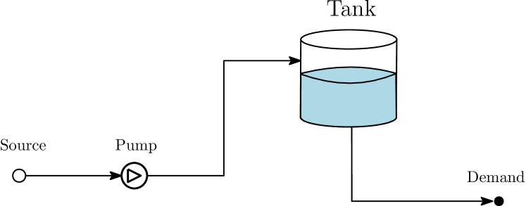
Figure 1: The topology of an aggregated water distribution system.

The dynamics of the water volume in the tank can be described using volume balance as

$$x_{k+1}=x_{k}+\Delta t\Big{(}u_{k}\left(r_{k},\alpha_{k}(x_{k}),x_{k}\right)-d_{k}\Big{)},$$ (1)

where $x\in\mathbb{R}$ denotes the water volume in the tank as the system state, $u\in\mathbb{R}$ denotes the pumping flow to the tank as the control input, and $d\in\mathbb{R}$ denotes the water demand as the exogenous input. $\Delta t$ is the sampling interval and $k\in\mathbb{N}$ denotes a discrete time instance.

The water demand $d_{k}$ is uncertain. In practice, periodicities in the water demand can usually be observed, for instance, a daily or weekly pattern. The control input $u_{k}\left(r_{k},\alpha_{k}(x_{k}),x_{k}\right)$ is determined based on the electricity price $r_{k}$ (considered as a stochastic variable) at time $k$, a price threshold $\alpha_{k}(x_{k})$ (to be designed) and the water volume in the tank $x_{k}$ at time $k$. $\overline{x}\leq V$ denotes a maximum water volume dictated by operational constraints while $\underline{x}>0$ denotes a minimum water volume to be kept in reserve. The control strategy is described as follows:

1. If the electricity price is equal or lower than the price threshold and the water volume in the tank is below or equal to an upper limit $\overline{x}$, then pumping occurs;

2. If the tank is close to empty, then pumping has to occur irrespective of electricity price in order to comply with a minimum water storage requirement;

3. Otherwise no pumping occurs.

Overall, this control strategy can be written as

$$u_{k}\left(r_{k},\alpha_{k}(x_{k}),x_{k}\right)=\begin{cases}q,&\text{if }r_{k}\leq\alpha_{k}(x_{k})\text{ and }x_{k}\leq\overline{x},\\ q,&\text{if }x_{k}\leq\underline{x},\\ 0,&\text{otherwise},\end{cases}$$ (2)

where $q$ denotes a constant flow provided by the pump.

Remark 1.

As water demands and electricity prices usually vary, the price threshold $\alpha_{k}(x_{k})$ is time-dependent and state-dependent, that is, at every time step, the price threshold could be different depending on time $k$ and the volume in the tank $x_{k}$.

An aggregated WDS has both capital and operating costs. The objective for the co-design problem is to minimize these costs by simultaneously designing the tank size $V$ and the control strategy while considering a long-term planning horizon $N>0$ (the number of discrete-time steps). The overall co-design cost is given by

$$c_{t}(V)+\sum_{k=0}^{N}\ell_{k}(r_{k},\alpha_{k}(x_{k}),x_{k}),$$ (3)

where the capital cost of the storage tank $c_{t}(V)$. The operating cost $\ell_{k}(r_{k},\alpha_{k}(x_{k}),x_{k})$ depends on the price, price threshold and state at each time $k$.

Since $r_{k}$ and $d_{k}$ are stochastic variables, the cost in (3) is a random variable. As $N$ is large, the long-term expected average cost is minimized, and the following co-design problem for the system in Fig. 1 is obtained.

$$\underset{\begin{subarray}{c}V,\;\alpha_{k}(x_{k}),\\ k=0,\ldots,N\end{subarray}}{\mathrm{minimize}}\;\;\frac{1}{N}c_{t}(V)+\mathbf{E}\left[\frac{1}{N}\sum_{k=0}^{N}\ell_{k}(r_{k},\alpha_{k}(x_{k}),x_{k})\right],$$ (4a)

subject to (1), (2) and

$$x_{0}=\tilde{x},$$ (4b)

$$0\leq x_{k}\leq V,\;k=0,\ldots,N,$$ (4c)

where $\tilde{x}$ denotes an initial water volume in the tank, which can also be treated as a stochastic variable with a certain distribution. The expectation is with respect to $r_{k}$, $d_{k}$ and $\tilde{x}$.

The co-design optimization problem (4) is difficult to solve for several reasons. The planning horizon $N$ could be long. It is typically based on the life cycle of the storage tank and planning horizons of 20, 50 and 100 years are common. Typical approaches to solve (4) such as Monte Carlo tree search become numerically unwieldy given the time scales.

III Stochastic Co-design Optimizations based on Finite-state Markov Chain

In this section, we formulate the stochastic optimization problem based on Markov chain theory to find the storage tank size $V$ and the price threshold $\alpha_{k}(x_{k})$. The reformulated optimization problem presented in this section is more tractable than (4) due to the approximations in the derivation of a finite-state Markov chain.

III-A Quantized Demands, Pumping Flows and Volumes

As introduced in Section II, water demands $d_{k}$ are time-varying and their distribution is periodic with period $T$. From the dynamics (1), it can be seen that the system state (water volume in the tank) depends on water demands. The introduced quantization of water demands and pumping flows allows us to represent the dynamics as a finite-state Markov chain.

Assumption 1.

The stochastic water demand $d_{k}$, $\forall k\in\mathbb{N}$ can take one of $m$ finite values, which can be represented as multiples of some positive scalar $d$, i.e.

$$d_{k}=\tau_{k}d\;\;\text{with probability of }a^{\tau_{k}}_{k},$$ (5)

where $\tau_{k}=0,1,\ldots,m-1$. Moreover, the water demands at different time instances are independent of each other. It holds $a^{\tau}_{k}=a^{\tau}_{k+T}$ for any $\tau=0,\ldots,m-1$. Furthermore, the probabilities $a^{\tau}_{k}$, $\tau=0,\ldots,m-1$ satisfy for every $k\in\mathbb{N}$,

$$a^{\tau}_{k}\geq 0,\allowdisplaybreaks$$ (6a)

$$\sum_{\tau=0}^{m-1}a^{\tau}_{k}=1.$$ (6b)

A close approximation of demands can be achieved if $d$ is chosen to be small, but it would lead to more states in the Markov chain.

We make the following assumption on the pumping flow.

Assumption 2.

The pumping flow $q$ is a multiple of $d$, i.e.

$$q=\zeta d,$$ (7)

where $\zeta>0$ is an integer.

From Assumption 2, it follows that the actual pumping flow in (2) can be reformulated as

$$u_{k}\left(r_{k},\alpha_{k}(x_{k}),x_{k}\right)=\zeta_{k}d,$$ (8)

where $\zeta_{k}=\zeta$ if pumping occurs, otherwise $\zeta_{k}=0$.

Let us define $\Delta x=d\Delta t$. It follows that at each time step there exists an integer $\gamma$ (positive, negative or zero) such that

$$x_{k+1}-x_{k}=\gamma d\Delta t=\gamma\Delta x.$$ (9)

In addition, the following two assumptions are made for establishing the Markov chain.

Assumption 3.

The total volume $V$, the volume limits $\overline{x}$, $\underline{x}$ and the initial water volume $\tilde{x}$ are multiples of $\Delta x$, i.e. $V=n\Delta x$, $\underline{x}=n_{p}\Delta x$, $\overline{x}=n_{s}\Delta x$ and $\tilde{x}=n_{0}\Delta x$, where $n$, $n_{p}$, $n_{s}$ and $n_{0}$ are integers.

Assumption 4.

The electricity prices $r_{k}$, $\forall k\in\mathbb{N}$ are stochastic and independent of each other. Moreover, they do admit probability densities $f_{k}(r_{k})$ that are periodically varying in time $k$ with a period of $T$. Furthermore, given $k$ the electricity prices are independent of water demands and initial water volume in the tank.

III-B Finite-state Markov Chain of Volume Evolution

From Assumptions 1-3, water volume in the tank is a multiple of $\Delta x$. Moreover, due to the independence assumptions (Assumptions 1 and 4), the dynamics (1) and the control strategy (2), $x_{k}$ can be represented as a finite state Markov chain, where the states in the Markov chain are represented by $(i,\kappa)$ with $\kappa=\mathrm{mod}(k,T)$ corresponding to the water volume in the tank as

$$x_{k}=i\Delta x.$$ (10)

Also from Assumption 3, the maximum value of $i$ is $n=\frac{V}{\Delta x}$ corresponding to a full tank while the minimum value is 0 corresponding to an empty tank.

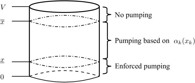
Figure 2: Labeled water volumes in the tank and associated control actions.

Fig. 2 shows water volumes with associated control actions using the control strategy (2). $\overline{x}$ is chosen such that the tank will not overflow if there is pumping and the water demand is zero, i.e. $n_{s}+\zeta\leq n$. Similarly, we also consider that the tank is large enough so that it does not empty if there is no pumping when the water volume in the tank is above $\bar{x}$ and the water demand is maximum, i.e. $n_{p}-m+2\geq 0$. The finite-state Markov chain proposed next considers not only the volume in the tank but also the current time within any given period, $T$. The total number of states in the Markov chain is $\bar{n}=(n+1)T$.

For every time $\kappa=\mathrm{mod}(k,T)$ over a period $T$, the pumping price thresholds can be written as $\alpha_{k}(x_{k})=\alpha_{\kappa}(i\Delta x)$ with $i=\frac{x_{k}}{\Delta x}$. The states in the Markov chain are shown in Fig. 3. The row represents a time between 0 and $T-1$ and the column represents water volumes in the tank between $0$ and $V$.

Figure 3: The states in the Markov chain for the co-design problem.

In the following, we discuss the transition probabilities for states in the Markov chain. The transition probabilities are denoted as $p_{\kappa}^{i,j}$ at time k from state $(i,\kappa)$ to state $(j,\mathrm{mod}(\kappa+1,T))$ at time $k+1$.

III-B1 States with no pumping

According to the control strategy introduced in (2), no pumping occurs when the water volume in the tank is above $\overline{x}=n_{s}\Delta x$.

Figure 4: States and transition probabilities when there is no pumping.

As shown in Fig. 4, for states $(i,\kappa)$, $i=n_{s}+1,\ldots,n$ for every $\kappa=0,\ldots,T-1$, the transition probabilities from state $(i,\kappa)$ to state $(i-\tau,\mathrm{mod}(\kappa+1,T))$ is

$$p^{i,i-\tau}_{\kappa} =a^{\tau}_{\kappa},\;\tau=0,1,\ldots,m-1,$$ (11)

where $a^{\tau}_{\kappa}$ is given in (5).

III-B2 States with pumping based on $\alpha_{\kappa}(i\Delta x)$

For states $(i,\kappa)$, $i=n_{p}+1,\ldots,n_{s}$ for every $\kappa=0,\ldots,T-1$, pumping occurs if $r_{k}\leq\alpha_{\kappa}(i\Delta x)$ with $\kappa=\mathrm{mod}(k,T)$.

Figure 5: States and transition probabilities with pumping based on $\alpha_{\kappa}(i\Delta x)$.

When $r_{k}\leq\alpha_{\kappa}(i\Delta x)$, pumping occurs. The next state $(j,\mathrm{mod}(\kappa+1,T))$ in the Markov chain when the water demand is $\tau d$, can be obtained from

$$j=i+\zeta-\tau.$$ (12)

Therefore, the transition probability from state $(i,\kappa)$ to state $(i+\zeta-\tau,\mathrm{mod}(\kappa+1,T))$ is

$$p^{i,i+\zeta-\tau}_{\kappa}=F_{\kappa}(\alpha_{\kappa}(i\Delta x))a^{\tau}_{\kappa},\;\tau=0,1,\ldots,m-1,$$ (13)

where $F_{\kappa}(\cdot)$ is the cumulative distribution function for electricity prices.

When $r_{k}>\alpha_{\kappa}(i\Delta x)$, no pumping occurs. The transition probability from state $(i,\kappa)$ to state $(i-\tau,\mathrm{mod}(\kappa+1,T))$ is

$$p^{i,i-\tau}_{\kappa}=\Big{(}1-F_{\kappa}(\alpha_{\kappa}(i\Delta x))\Big{)}a^{\tau}_{\kappa},\;\tau=0,1,\ldots,m-1.$$ (14)

III-B3 States with enforced pumping

According to the control strategy introduced in (2), enforced pumping is triggered when the water volume in the tank is at or below $\underline{x}=n_{p}\Delta x$.

Figure 6: States and transition probabilities with enforced pumping.

As shown in Fig. 6, for states $(i,\kappa)$, $i=0,1,\dots,n_{p}$ for every $\kappa=0,\ldots,T-1$, due to that the enforced pumping occurs, the next state in the Markov chain when the water demand is $\tau d$, can be found from

$$j=\max\left(0,i+\zeta-\tau\right).$$ (15)

Therefore, the transition probability from state $(i,\kappa)$ to state $(j,\mathrm{mod}(\kappa+1,T))$ is

$$p^{i,j}_{\kappa}=\begin{cases}a^{i+\zeta-j}_{\kappa},&\text{if }0<j<i+\zeta-1,\\ \displaystyle\sum_{\tau=i+\zeta}^{m}a^{\tau}_{\kappa},&\text{if }j=0.\end{cases}$$ (16)

By stacking the states in Fig. 3 row by row into a state vector, the following transition probability matrix is obtained

$$\mathbf{P}=\begin{bmatrix}\mathbf{0}&P_{0}&\mathbf{0}&\ldots&\mathbf{0}&\mathbf{0}\\ \mathbf{0}&\mathbf{0}&P_{1}&\ldots&\mathbf{0}&\mathbf{0}\\ \vdots&\vdots&\vdots&\ddots&\vdots&\vdots\\ \mathbf{0}&\mathbf{0}&\mathbf{0}&\ldots&P_{T-2}&\mathbf{0}\\ P_{T-1}&\mathbf{0}&\mathbf{0}&\ldots&\mathbf{0}&\mathbf{0}\end{bmatrix},$$ (17)

where for $\kappa=0,\ldots,T-1$,

$$P_{\kappa}=\begin{bmatrix}p^{0,0}_{\kappa}&\ldots&p^{0,n}_{\kappa}\\ \vdots&\ddots&\vdots\\ p^{n,0}_{\kappa}&\ldots&p^{n,n}_{\kappa}\end{bmatrix},$$ (18)

and the transition probabilities $p^{i,j}_{\kappa}$, $i,j=0,1,\ldots,n$, $\kappa=0,\ldots,T-1$ are given in (11), (13), (14) and (16).

We make the following assumption on $\mathbf{P}$.

Assumption 5.

The transition matrix $\mathbf{P}$ in (17) is irreducible.

This assumption means that any state in the Markov chain can be reached from any other state in a finite number of steps with positive probability. This is a very mild assumption, which essentially means that any water volume $i\Delta x$ can be reached from any starting volume $j\Delta x$.

For this Markov chain, the stationary probabilities of the states stacked in the vector $\bm{\pi}=[\pi^{i}_{\kappa},i=0,\ldots,n,\kappa=0,\ldots,T-1]$ can be obtained from the balance and normalization equations:

$$\bm{\pi} =\mathbf{P}^{\top}\bm{\pi},$$ (19a)

$$1 =\mathbf{1}_{\bar{n}}^{\top}\bm{\pi},$$ (19b)

where $\mathbf{1}_{\bar{n}}$ is a vector with all $\bar{n}=(n+1)T$ elements equal to 1.

For an irreducible $\mathbf{P}$, the stationary probabilities are unique. Let $\ell_{k}(r_{k},\alpha_{k}(x_{k}),x_{k}):\mathbb{R}^{3}\rightarrow\mathbb{R}$ be the operating cost function at time $k$ in (4a) and let $W(N):\mathbb{N}_{+}\rightarrow\mathbb{R}$ be the time average operating cost

$$W(N):=\frac{1}{N}\sum_{k=0}^{N-1}\ell_{k}(r_{k},\alpha_{k}(x_{k}),x_{k}),$$ (20)

where $N>0$ is the time horizon.

Theorem 1.

Assume that the cost functions $\ell_{k}(r_{k},\alpha_{k}(x_{k}),x_{k})$ have finite second order moments for given $\alpha_{k}(x_{k})$ and $x_{k}$. Define $\bar{\ell}$ as

$$\bar{\ell}:=\sum_{\kappa=0}^{T-1}\sum_{i=0}^{n}\pi_{\kappa}^{i}\bar{\ell}_{\kappa}(\alpha_{\kappa}(i\Delta x),i\Delta x),$$ (21)

where $\bar{\ell}_{\kappa}(\alpha_{\kappa}(i\Delta x),i\Delta x)=\mathbf{E}(\ell_{\kappa}(r_{\kappa},\alpha_{\kappa}(i\Delta x),i\Delta x))$ and the expectation is with respect to $r_{\kappa}$. Then, using the control strategy (2) under Assumptions 1-5, it holds that for any distribution of initial states,

$$\mathbf{Pr}\left\{\lim_{N\rightarrow\infty}W(N)=\bar{\ell}\right\}=1.$$ (22)

Proof.

Denote the states in the Markov chain by $z_{k}=[z_{1_{k}},z_{2_{k}}]^{\top}:=\left[\frac{x_{k}}{\Delta_{x}},\mathrm{mod}(k,T)\right]^{\top}$. It follows that $z_{k+1}=\left[z_{1_{k}}+\zeta_{k}-\tau_{k},\mathrm{mod}(z_{2_{k}}+1,T)\right]^{\top}$.

From (20), we have

$$W(N)=\frac{1}{N}\sum_{k=0}^{N-1}\ell_{z_{2_{k}}}(r_{k},\alpha_{z_{2_{k}}}(z_{1_{k}}\Delta x),z_{1_{k}}\Delta x).$$

Let $\mathbf{I}_{i,\kappa}(z_{k})$ be the indicator function:

$$\mathbf{I}_{i,\kappa}(z_{k})=\begin{cases}1&\text{if }z_{1_{k}}=i\text{ and }z_{2_{k}}=\kappa,\\ 0&\text{otherwise. }\end{cases}$$

Then, the average operating cost is equivalent to

$$W(N) =\frac{1}{N}\sum_{k=0}^{N-1}\sum_{\kappa=0}^{T-1}\sum_{i=0}^{n}\mathbf{I}_{i,\kappa}(z_{k})\ell_{\kappa}(r_{k},\alpha_{\kappa}(z_{1_{k}}\Delta x),z_{1_{k}}\Delta x)$$

$$=\frac{1}{N}\sum_{k=0}^{N-1}\sum_{\kappa=0}^{T-1}\sum_{i=0}^{n}\mathbf{I}_{i,\kappa}(z_{k})\ell_{\kappa}(r_{k},\alpha_{\kappa}(i\Delta x),i\Delta x),$$

where the second inequality holds due to the indicator function $\mathbf{I}_{i,\kappa}(z_{k})$.

$s_{i,\kappa}=\sum_{k=0}^{N-1}\mathbf{I}_{i,\kappa}(z_{k})$ is the number of times the state $(i,\kappa)$ has been visited over the time horizon $N$. Let $\tilde{k}_{i,\kappa}(l)$ be the time index when the state $(i,\kappa)$ is visited for the $l$-th time. It follows that for fixed $i$ and $\kappa$

$$\frac{1}{N}\sum_{k=0}^{N-1}\mathbf{I}_{i,\kappa}(z_{k})\ell_{\kappa}(r_{k},\alpha_{\kappa}(i\Delta x),i\Delta x)$$

$$= \frac{s_{i,\kappa}}{N}\cdot\frac{1}{s_{i,\kappa}}\sum_{l=0}^{s_{i,\kappa}}\ell_{\kappa}(r_{\tilde{k}_{i,\kappa}(l)},\alpha_{\kappa}(i\Delta x),i\Delta x).$$

From Assumption 5 and [25, Theorem 1.9.7], $\frac{s_{i,\kappa}}{N}\rightarrow\pi_{\kappa}^{i}$ with probability 1 as $N\rightarrow\infty$. It follows that $s_{i,\kappa}\rightarrow\infty$ as $N\rightarrow\infty$ when $\pi_{\kappa}^{i}>0$. Under Assumptions 1 and 4 and due to that $z_{k}$ only depends on $z_{k-1}$, $r_{k-1}$ and $d_{k-1}$, $r_{k}$ is independent of $z_{k},z_{k-1},\ldots,z_{0}$. Therefore, $\ell_{\kappa}(r_{\tilde{k}_{i,\kappa}(l)},\alpha_{\kappa}(i\Delta x),i\Delta x)$, $l=1,2,\ldots$ is a sequence of independent random variables.

As $l_{\kappa}$ has finite second order moment, from Kolmogorov’s strong law of large numbers [22, Theorem 4.3.2], it follows that

$$\frac{1}{s_{i,\kappa}}\sum_{l=0}^{s_{i,\kappa}}\ell_{\kappa}(r_{\tilde{k}_{i,\kappa}(l)}, \alpha_{\kappa}(i\Delta x),i\Delta x)$$

$$\rightarrow\; \mathbf{E}(\ell_{\kappa}(r_{\kappa},\alpha_{\kappa}(i\Delta x),i\Delta x))$$

with probability 1 as $s_{i,\kappa}\rightarrow\infty$.

Therefore, from the above, we have

$$W(N)\rightarrow\sum_{\kappa=0}^{T-1}\sum_{i=0}^{n}\pi_{\kappa}^{i}\mathbf{E}(\ell_{\kappa}(r_{\kappa},\alpha_{\kappa}(i\Delta x),i\Delta x))=\bar{\ell}$$

with probability 1 as $N\rightarrow\infty$. ∎

Theorem 1 is useful for investigating the operating cost over a long horizon in a computationally efficient manner. The cost $\bar{\ell}$ in (21) will be used in the next subsection to approximate the operating cost. Note that the result in Theorem 1 does not depend on the initial state of the Markov chain. Therefore, the constraint (4b) is omitted in the formulation in the following subsection. Furthermore, one iteration of the Markov chain takes one discrete-time sampling interval, such that there is a one-to-one correspondence between the real-time and the iteration index in the Markov chain.

III-C Stochastic Co-design Formulation

Considering the Markov chain described above, we next reformulate the co-design cost function. The decision variables in the co-design optimization are the tank size $V$ and the vector of state-dependent price thresholds $\bm{\alpha}=[\alpha_{\kappa}(i\Delta x),i=n_{p}+1,\ldots,n_{s},\kappa=0,\ldots,T-1]$.

III-C1 Capital Cost

The capital cost of a storage tank, $c_{t}(V)$, is a deterministic and monotonic function of volume.

III-C2 Operating Cost

The operating cost includes two parts: the pumping energy cost and a penalty cost when the tank is empty or close to empty. The total pumping cost over the planning horizon of $N$ time samples can be evaluated by the following two energy costs:

• When the volume is $n_{p}\Delta x$ or lower, enforced pumping occurs based on the control strategy in (2). In this case, the pump operates regardless of the price. The expected pumping energy cost is

  $$\bar{\ell}^{e}_{\kappa}(\alpha_{\kappa}(i\Delta x),i\Delta x)=\varepsilon_{p}\mu_{\kappa},$$ (23)

  for $\kappa=0,\ldots,T-1$ and $i=0,\ldots,n_{p}$, otherwise $\bar{\ell}^{e}_{\kappa}(\alpha_{\kappa}(i\Delta x),i\Delta x)=0$, where $\varepsilon_{p}$ denotes the energy consumption for pumping in a sampling interval when the pump is operating. $\mu_{\kappa}$ is the expected value of the electricity price at time $\kappa=\mathrm{mod}(k,T)$.

• When the volume is between $(n_{p}+1)\Delta x$ and $n_{s}\Delta x$, pumping occurs only when the price is below a threshold. The expected pumping energy cost is

  $$\bar{\ell}^{r}_{\kappa}(\alpha_{\kappa}(i\Delta x),i\Delta x)=\bar{p}^{i}_{\kappa}\varepsilon_{p}\bar{c}_{\kappa}(\alpha_{\kappa}(i\Delta x)),$$ (24)

  for $\kappa=0,\ldots,T-1$ and $i=n_{p}+1,\ldots,n_{s}$, otherwise $\bar{\ell}^{r}_{\kappa}(\alpha_{\kappa}(i\Delta x),i\Delta x)=0$, where

  $$\bar{c}_{\kappa}(\alpha_{\kappa}(i\Delta x)) =\int_{-\infty}^{\alpha_{\kappa}(i\Delta x)}rf_{\kappa}(r)dr,$$ (25a)

  $$\bar{p}^{i}_{\kappa} =F_{\kappa}(\alpha_{\kappa}(i\Delta x)),$$ (25b)

  and $\bar{c}_{\kappa}(\alpha_{\kappa}(i\Delta x))$ is the expected value of the electricity price given that it is less than $\alpha_{\kappa}(i\Delta x)$. $\bar{p}^{i}_{\kappa}$ denotes the probability that the pump is operating.

Remark 2.

If the electricity prices are Gaussian random variables with mean $\mu$ and variance $\sigma^{2}$, then the expected value of the electricity price given that it is less than or equal to $\alpha_{\kappa}(i\Delta x)$ is

$$\bar{c}(\alpha_{\kappa}(i\Delta x)) =\mathbf{E}\left[r\mid r\leq\alpha_{\kappa}(i\Delta x)\right]$$

$$=\mu-\sigma^{2}\frac{f(\alpha_{\kappa}(i\Delta x))}{F(\alpha_{\kappa}(i\Delta x))}.$$

Furthermore, low tank water volumes, especially an empty tank, should be avoided as they compromise the ability of the WDS to meet demand and are associated with a penalty. To incorporate this, a penalty cost when the volume of water is below $n_{r}\Delta x$ ($n_{r}\geq 0$) is applied. The penalty cost is given by

$$\bar{\ell}^{p}_{\kappa}((\alpha_{\kappa}(i\Delta x),i\Delta x)=w,$$ (26)

for $\kappa=0,\ldots,T-1$ and $i=0,\ldots,n_{r}$, otherwise $\bar{\ell}^{p}_{\kappa}((\alpha_{\kappa}(i\Delta x),i\Delta x)=0$, where $w$ is a weight. The penalty applies every time instant the volume in the tank is below $n_{r}\Delta x$.

The co-design problem in (4a) is

$$\underset{V,\alpha_{k}(x_{k}),k=0,\ldots,N}{\mathrm{minimize}}\;\;\frac{1}{N}c_{t}(V)+\mathbf{E}\left[\frac{1}{N}\sum_{k=0}^{N}\ell_{k}(r_{k},\alpha_{k}(x_{k}),x_{k})\right].$$

From Theorem 1, the operating cost

$$\frac{1}{N}\sum_{k=0}^{N}\ell_{k}(r_{k},\alpha_{k}(x_{k}),x_{k})$$

converges with probability 1 to

$$\bar{\ell}(\bm{\alpha},V)=\sum_{\kappa=0}^{T-1}\sum_{i=0}^{n}\pi_{\kappa}^{i}\bar{\ell}_{\kappa}(\alpha_{\kappa}(i\Delta x),i\Delta x),$$ (27)

with

$$\bar{\ell}_{\kappa}(\alpha_{\kappa}(i\Delta x),i\Delta x)= \bar{\ell}^{e}_{\kappa}(\alpha_{\kappa}(i\Delta x),i\Delta x)+\bar{\ell}^{r}_{\kappa}(\alpha_{\kappa}(i\Delta x),i\Delta x)$$

$$+\bar{\ell}^{p}_{\kappa}((\alpha_{\kappa}(i\Delta x),i\Delta x),$$

where $\bar{\ell}^{e}_{\kappa}(\cdot)$, $\bar{\ell}^{r}_{\kappa}(\cdot)$ and $\bar{\ell}^{p}_{\kappa}(\cdot)$ are given in (23), (24) and (26).

As Theorem 1 holds for any distribution for initial states, the constraint (4b) is automatically satisfied. The constraint (4c) also holds for given assumptions in the Markov chain. Therefore, the co-design problem (4) can be reformulated as

$$\underset{\bm{\alpha},V}{\mathrm{minimize}}\;\; \frac{1}{N}c_{t}(V)+\bar{\ell}(\bm{\alpha},V),$$ (28)

where $\bar{\ell}(\bm{\alpha},V)$ is given in (27) and $\bm{\alpha}=[\alpha_{\kappa}(i\Delta x),i=n_{p}+1,\ldots,n_{s},\kappa=0,\ldots,T-1]$.

III-D Stochastic Co-design Algorithm

From the co-design formulation in (28), it can be seen that the number of decision variables in the vector $\bm{\alpha}$ depends on the tank size $V$. As the tank size $V$ increases, the number of states in the Markov chain increases. Therefore, the number of price pumping thresholds (elements in $\bm{\alpha}$) also increases, thereby changing the dimension of the optimization problem.

For a given tank size $V_{\eta}$ with $\eta=1,\ldots,s$, the optimization problem (28) is solved by a numerical optimization algorithm, e.g. simultaneous perturbation stochastic approximation (SPSA) [26]. Then, the tank size $V$ and the corresponding $\alpha$ that minimizes the co-design cost are obtained. We summarize the above procedure in Algorithm 1.

Algorithm 1 Stochastic Co-design of Storage and Control

1:Given possible tank sizes $V_{1},\ldots,V_{s}$;

2:for $\eta=1:s$ do

3:     $\bm{\alpha}_{\eta}:=\underset{\bm{\alpha}}{\arg\min}\;\bar{\ell}(\bm{\alpha},V_{\eta})$;

4:     $J_{\eta}:=c_{t}(V_{\eta})+N\bar{\ell}(\bm{\alpha}_{\eta},V_{\eta})$;

5:end for

6:Obtain the minimum co-design cost $J^{*}$ over all the possible tank sizes by $J^{*}:=\min(J_{1},\ldots,J_{s})$;

7:Extract the optimal price threshold $\bm{\alpha}^{*}$ and tank size $V^{*}$ corresponding to $J^{*}$.

IV Illustrative Examples

In this section, we provide three examples illustrating the proposed co-design method. In these three examples, the electricity prices are Gaussian random variables $r\sim\mathcal{N}(20,10)$. The period is $T=1$, i.e. the distributions of water demand and electricity price do not vary with time. The capital cost of the storage tank is $c_{v}=10,000$ per unit volume. The planning horizon is chosen as $20$ years that corresponds to $N=175,200$ samples using a sampling time interval of $\Delta t=1$ hour. In the first example, the price threshold is state independent and hence constant. In the second and third examples, state-dependent price pumping thresholds are considered.

IV-A State-independent Price Threshold and Constant Demand

$$\pi^{0}=\begin{cases}\frac{1}{2V},&\text{if }\alpha=\mu,\\ \frac{F(\alpha)\left(1-2F(\alpha)\right)\left(1-F(\alpha)\right)^{V-1}}{F(\alpha)(1-2F(\alpha))(1-F(\alpha))^{V-1}+F(\alpha)^{V}(1-2F(\alpha))+F(\alpha)(1-F(\alpha))^{V-1}-F(\alpha)^{V}},&\text{otherwise}.\end{cases}$$ (29)

 

We first consider the case where the water demand is constant $d_{k}=d=1$ volume unit per sampling interval. The pumping inflow is $q=2$ volume unit per sampling interval when the pump is operating. The possible tank volume, $x$, ranges between 0 and a positive integer $V$. We consider the control strategy described in (2) with state-independent price threshold $\alpha$ and $\underline{x}=0$ and $\overline{x}=V$. The corresponding Markov chain is shown in Fig. 7. The transition probabilities $p=F(\alpha)$ are the same since $\alpha$ is state-independent, where $F(\cdot)$ is the CDF of the Gaussian distribution.

Figure 7: Markov chain for the example with state-independent price threshold and constant demand.

The Markov chain in Fig. 7 is irreducible and has a unique communicating class that contains all the states if $0<p<1$.

The stationary probabilities depend on pumping probability $p$. The stationary probabilities of the states, denoted by $\pi^{i}$, $i=0,1,\ldots,V$, can be obtained from the following normalization and balance equations:

$$\sum_{i=0}^{V}\pi^{i}=1,\allowdisplaybreaks$$

$$\pi^{0}=(1-p)\pi^{1},\allowdisplaybreaks$$

$$\pi^{i}=p\pi^{i-1}+(1-p)\pi^{i+1},\;\;i=1,\ldots,V-2,\allowdisplaybreaks$$

$$\pi^{V-1}=p\pi^{V-2}+\pi^{V},\allowdisplaybreaks$$

$$\pi^{V}=p\pi^{V-1}.\allowdisplaybreaks$$

For this example, we can explicitly derive an analytical expression for $\pi^{0}$ for the state $x=0$ parameterized by $\alpha$ and $V$. This expression is given in (29) and can be used to find the stationary probabilities for the remaining states $\pi^{i}$.

The operating cost can be divided into two cases: one due to enforced pumping with probability 1 from zero state $i=0$; and pumping based on the price threshold $\alpha$ with probability $p=F(\alpha)$. Following the steps in Section III-C with $n_{r}=0$, the expected operating cost is thus given by

$$\bar{\ell}(\alpha,V)= \pi^{0}(\alpha,V)(\varepsilon_{p}\mu+w)$$

$$+\sum_{i=1}^{V-1}\pi^{i}(\alpha,V)p\varepsilon_{p}\bar{c}(\alpha),$$ (30)

where $\bar{c}(\alpha)=\mu-\sigma^{2}\frac{f(\alpha)}{F(\alpha)}$ and $\varepsilon_{p}$ is the energy consumption in a sampling interval when the pump is operating.

Then, the stochastic co-design optimization problem can be formulated as follows:

$$(\alpha^{*},V^{*}) :=\underset{\alpha,V}{\arg\min}{\;\;\frac{1}{N}c_{v}V}+\bar{\ell}(\alpha,V),$$ (31)

where $\bar{\ell}(\alpha,V)$ is given in (IV-A).

The parameters are given as $\varepsilon_{p}=1$ and $w=0$. Using the expression for $\pi^{0}(\alpha,V)$ in (29), the co-design optimization problem (31) can easily be solved. The co-design cost surface is shown in Fig. 8. It can be seen that the optimization problem is non-convex but has a unique minimum, allowing for targeted numerical optimization routines to be deployed.

The optimized parameters and costs are reported in Table I. Not surprisingly, the optimal state-independent $\alpha^{*}$ is equal to the mean $\mu=20$, which gives a pumping probability of $p=0.5$. Next, we will compare these results to the case where the price thresholds are state-dependent.

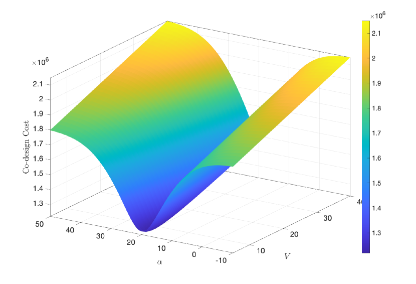
Figure 8: The co-design cost surface for a state-independent price threshold and constant demand.

TABLE I: Co-design solutions of three examples.

	State-independent price threshold	State-dependent price thresholds	State-dependent price thresholds
	Constant demand	Constant demand	Uncertain demands
Optimal tank size $V^{*}$	8	8	9.6
Optimal price threshold $\alpha^{*}$	20	see Fig. 10(a)	see Fig. 10(b)
Optimal capital cost	80,000	80,000	96,000
Optimal operating cost over $N$	1,140,421	1,105,603	1,105,112
Optimal co-design cost $N$	1,220,421	1,185,603	1,201,112

IV-B State-dependent Price Thresholds and Constant Demand

Here, the setting is the same as before, apart from that the electricity price thresholds are state-dependent. The Markov chain with transition probabilities is shown in Fig. 9.

Figure 9: Markov chain for the example with state-dependent price thresholds and constant demand.

The Markov chain in Fig. 9 is irreducible if all the transition probabilities $0<p(\alpha(i))<1$, $i=1,\ldots,V-1$. The stationary probabilities for each state in the Markov chain can be obtained by solving the normalization and balance equations.

As in the previous example (with $n_{r}=0$), we follow the steps in Section III-C and obtain the following co-design optimization problem:

$$(\bm{\alpha}^{*},V^{*}):= \underset{\bm{\alpha},V}{\arg\min}\;\;{c_{v}V}$$

$$+\pi^{0}(\bm{\alpha},V)(\varepsilon_{p}\mu+w)$$

$$+\sum_{i=1}^{V-1}\pi^{i}(\bm{\alpha},V)p(\alpha(i\Delta x))\varepsilon_{p}\bar{c}(\alpha(i\Delta x)),$$ (32)

where $p(\alpha(i\Delta x))=F(\alpha(i\Delta x))$, $\Delta x=d\Delta t=1$ and $\bm{\alpha}=[\alpha(i\Delta x),i=1,\ldots,V-1]$.

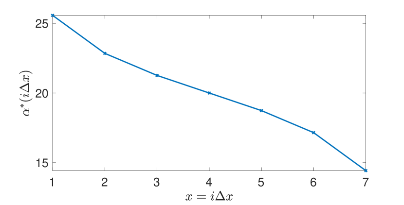
(a) With constant demand

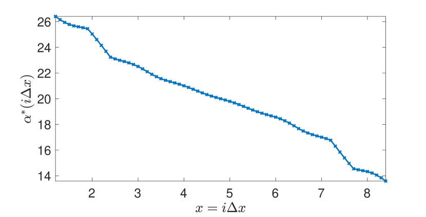
(b) With uncertain demands

Figure 10: The optimal state-dependent price thresholds $\alpha^{*}(i\Delta x)$.

As the number of optimization parameters has increased due to state-dependent $\alpha(i\Delta x)$, the co-design surface can no longer be plotted, but a numerical solution can still be found. To obtain the solution to the co-design optimization problem (IV-B), we utilize Algorithm 1 with the SPSA method proposed in [26]. The optimal solutions and costs are presented in Table I and the optimal state-dependent price thresholds are shown in Fig. 10(a). The observed trend reveals that as the volume in the tank increases, the threshold decreases. This trend is logical because when the volume in the tank is low, having larger threshold results in higher transition probabilities to higher volume states, consequently reducing the probabilities of transitioning to an even lower volume, which could potentially incur a significant operating cost due to enforced pumping (and additional penalties for running empty, although in this example $w=0$, so no explicit penalty is applied for running empty or below a given threshold volume). Similarly, when the volume is high there is less need to pump, and subsequently, a smaller price threshold can be set.

Compared to the result in the previous example, the infrastructure cost is the same, but a lower co-design cost is achievable through the additional degrees of freedom available in the operating strategy.

IV-C State-dependent Price Thresholds and Uncertain Demands

To consider a more realistic example, the water demands are now uncertain:

$$d_{k}=\begin{cases}0.8&\text{with probability of }0.2,\\ 0.9&\text{with probability of }0.2,\\ 1&\text{with probability of }0.2,\\ 1.1&\text{with probability of }0.2,\\ 1.2&\text{with probability of }0.2,\\ \end{cases}$$

for $k=1,\ldots,N$. Note the average demand is the same as in the previous examples. The demand quantization interval is chosen as $d=0.1$ and the state quantization interval is $\Delta x=0.1$.

Following the procedures in the previous example, the co-design optimization is formulated as follows:

$$(\bm{\alpha}^{*},V^{*}) :=\underset{\bm{\alpha},V}{\arg\min}\;\;{c_{v}V}$$

$$\;+\pi^{0}(\bm{\alpha},V)(\varepsilon_{p}\mu+w)+\sum_{j=1}^{n_{p}}\pi^{j}(\bm{\alpha},V)\varepsilon_{p}\mu$$

$$\;+\sum_{i=n_{p}+1}^{n_{s}}\pi^{i}(\bm{\alpha},V)p(\alpha(i\Delta x))\varepsilon_{p}\bar{c}(\alpha(i\Delta x)),$$ (33)

where $p(\alpha(i\Delta x))=F(\alpha(i\Delta x))$, $n_{p}=\frac{\underline{x}}{\Delta x}$ and $n_{s}=\frac{\overline{x}}{\Delta x}$ with $\underline{x}=1.2$ and $\overline{x}=V-1.2$. $\bm{\alpha}=[\alpha(i\Delta x),i=n_{p}+1,\ldots,n_{s}]$.

We again utilize Algorithm 1 with the SPSA method to find the optimal co-design parameters reported in Table I and Fig. 10(b). It is interesting to note that the state-dependent price threshold trend is very similar to the constant demand example, but the uncertain demand induces a more conservative infrastructure solution. Due to the larger tank, the operating cost is actually reduced compared to when the demand was constant.

IV-D Sensitivity Analysis

In this section, we investigate the sensitivity of the results in the last example with respect to variations in the distribution of energy prices. Two cases are considered:

In the first case, the sensitivity of the operating cost obtained from the optimal co-design solution with respect to the price distribution is investigated. The system is co-designed using constant assumed parameters $\bar{\mu}$ and $\bar{\sigma}$, but the true parameters $\mu$ and $\sigma$ are different from the assumed values.

In the second case, the sensitivity of the achievable cost with the true parameters with respect to the assumed price distribution used in the co-design is investigated. The co-design is carried out for different parameters $\bar{\mu}$ and $\bar{\sigma}$ while the actual values $\mu$ and $\sigma$ are always kept constant.

IV-D1 Sensitivity of Operating Cost to Changes in Actual Electricity Prices

Using Algorithm 1 with price distribution $\mathcal{N}(\bar{\mu},\bar{\sigma})$ ($\bar{\mu}=20$ and $\bar{\sigma}=10$), the optimal co-design solutions are reported in Table I and Fig. 10. Using the obtained price thresholds, simulations with different $\mu$ and $\sigma$ have been carried out with the same tank size $V^{*}=9.6$. The results are shown in Table II.

The empirical operating cost in the simulations with $\mu=\bar{\mu}$ and $\sigma=\bar{\sigma}$, obtained from Table II, aligns with the optimal operating cost from the co-design optimization in Table I.

TABLE II: Sensitivity results of operating cost to changes in actual electricity prices for fixed tank volume of 9.6.

$\mu$	$\sigma$	Empirical Oper. Cost	Oper. Cost Diff.
20	10	1,105,901	0.00%
20	20	475,511	-57.00%
20	5	1,435,423	29.79%
24	10	1,508,731	36.42%
24	20	874,863	-20.89%
24	5	1,821,642	64.72%
16	10	803,050	-27.39%
16	20	169,642	-84.66%
16	5	1,117,713	1.06%

• Operating cost difference is compared to the operating cost with $\mu=20$ and $\sigma=10$ in the first row.

TABLE III: Sensitivity results of total co-design cost to changes in electricity price distribution.

$\tilde{\mu}$	$\tilde{\sigma}$	$V^{*}$	Capital Cost	Empirical Oper. Cost	Total Cost	Cost Diff.
20	10	9.60	96,000	1,106,423	1,202,423	0.00%
20	20	12.30	123,000	1,095,414	1,218,414	1.33%
20	5	7.50	75,000	1,144,921	1,219,921	1.46%
24	10	9.60	96,000	1,153,535	1,249,535	3.92%
24	20	12.30	123,000	1,111,422	1,234,422	2.66%
24	5	7.50	75,000	1,215,013	1,290,013	7.28%
16	10	9.60	96,000	1,157,641	1,253,641	4.26%
16	20	12.30	123,000	1,112,720	1,235,720	2.77%
16	5	7.50	75,000	1,218,631	1,293,631	7.59%

• Total cost difference is computed based on the sum of capital cost and empirical operating cost with $\tilde{\mu}=20$ and $\tilde{\sigma}=10$.

Table II shows that if the mean price $\mu$ increases (or decreases) by 20% from the mean used in design ($\tilde{\mu}=20$), the operating cost is increased (or decreased) by a larger amount (36% or -28% respectively). Similarly, we note that the variance of the electricity price has a significant impact on the operating cost if there is a large deviation from the value used during the design.

In summary, we can conclude that the actual operating cost can increase or decrease significantly if the actual price distribution is different from the one used during the design.

IV-D2 Sensitivity of Co-design Optimization to Changes in Electricity Price Distributions

Here we investigate the sensitivity of the co-design method by fixing the encountered price distribution at $\mu=20$ and $\sigma=10$, and using incorrect parameters $\tilde{\mu}$ and $\tilde{\sigma}$ during the design.

For each pair $(\tilde{\mu},\tilde{\sigma})$, the obtained $\bm{\alpha}^{*}$ and $V^{*}$ were used in 100 Monte Carlo simulations with true electricity prices described by a Gaussian distribution with $\mu=20$ and $\sigma=10$. The results are reported in Table III.

For cases with the same $\tilde{\sigma}=10$ but increased $\tilde{\mu}$, fewer enforced pumpings are triggered and as expected more time is spent in high tank volume states, as observed in Fig. 11. The converse is also true when $\tilde{\mu}$ is decreased. Nonetheless, the overall cost difference is relatively low, and the capital cost is the same in each case.

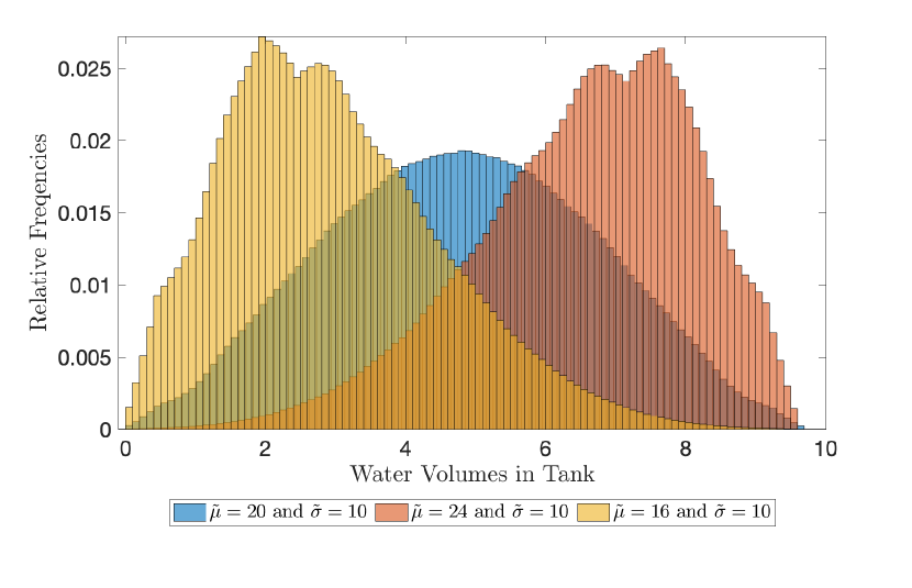
Figure 11: Comparison of relative frequencies from the Monte Carlo analysis with different $\tilde{\mu}$.

As can be seen from Table III, the total actual cost is rather insensitive to the price distribution used during the design phase, that is the obtained $V$ and $\alpha(i\Delta x)$ also work well when the actual price distribution is different. The largest difference occurs when the standard deviation $\tilde{\sigma}$ is underestimated, and this is due to that the co-design optimization selects a smaller tank size which leads to more frequent enforced pumping events.

To conclude, the first case investigated in Section IV-D1 shows that the operating cost achieved in the design phase is sensitive with respect to variations in the assumed price distribution. The results in this section show that, even if we had known the true distribution, we would not have been able to improve significantly on the actual cost.

V Case Study: a Water Network in South Australia

In this section, we apply the proposed co-design method to a high-fidelity simulation of a real-world water network in South Australia, operated by the South Australian Water Corporation (SA Water). We first describe the system and then present the data processing procedure for obtaining the parameters required for solving the co-design optimization problem. Then, we describe the simulation setup, which makes use of an EPANET hydraulic model. Finally, we evaluate the effectiveness of the solutions through a comparison with historic operational data from 2019.

V-A Description

The network topology is aggregated to be consistent with that shown in Fig. 1, so that it includes a pumping station with one pump, one storage tank, and an aggregated demand sector representing the combined demand of all downstream sectors. The co-design objective is to determine the optimal combined tank size and the price thresholds for operating the pumping station using the control strategy in (2).

For this water network, pumping flows and water demands in 2019 are available. The SA electricity prices in 2019 are available from the AEMO with a sampling time of 30 minutes [27]. As shown in Fig. 12, the water demand increases in the warmer months since the network services popular holiday area. The year was therefore divided into a summer period from November to April and a winter period from May to October.

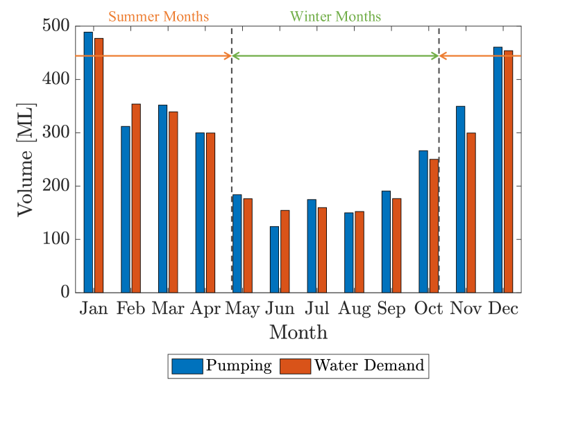
Figure 12: Monthly pumping and water demand from historical data with operation by SA Water using a trigger-level control.

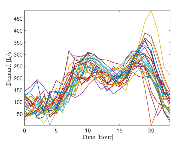
Figure 13: Typical summer-month daily water demands in January 2019 from historical data.

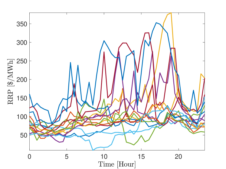
Figure 14: Typical South Australian electricity retail prices during January 2019 sourced from [28].

The following parameters were set based on available data:

• When the pump operates, the flow is $q=215$ L/s.

• Water demand has a noticeable daily pattern shown in Fig. 13. The period $T=24$ hours is therefore used.

• The quantization interval is chosen as $d=43$ L/s, and the quantized water demands for summer and winter months are chosen as $\tau d$ with $\tau=1,\ldots,11$. The corresponding probabilities $a_{\kappa}^{\tau}$ of demands were estimated for every $\kappa=\mod(k,T)=0,\ldots,23$.

• SA Water purchase electricity directly from the electricity market, with prices available in the AEMO database [28]. Some examples of how electricity prices vary over a 24-hour period are shown in Fig. 14. Extreme price events, which are taken to be when prices are above $500 per MWh, are removed for investigating price distributions. While actual price histories are used in the simulation, for the design they are assumed to be independently and identically distributed Gaussian random variables. Two distributions can be estimated by using data in the summer and winter months, respectively. For summer months, the mean electricity price is $\mu=\$89.77$/MWh and the standard deviation is $\sigma=\$43.39$/MWh while for winter months, $\mu=\$78.57$/MWh and $\sigma=\$42.58$/MWh.

• Water storage tanks with different sizes are considered in the co-design problem. Overall, the life cycle of the tank is taken to be 50 years [29]. The options for tank sizes are 3, 4, 5, 8, 10, 15 and 20 ML. The corresponding capital costs can be found in Table IV based on the numbers reported in [30].

• The penalty cost is $10,000 per times when the tank is empty, that is, $w=10,000$.

V-B Closed-loop Simulation Results

As the infrastructure lifetime is set to 50 years, the operating cost is found by using the summer and winter parameters for 25 years each. For each tank size, the total cost is found by adding the capital cost and the operating cost. The results are reported in Table IV. As also shown in Fig. 15, it can be seen that a smaller tank size may save on capital costs but leads to higher operating and penalty costs. When the tank is too small, the risk of having less water in the tank than the minimum allowed increases. A larger tank provides more flexibility in storing water and meeting demands during high-priced times, but the savings in operating costs may not compensate for the increase in capital costs.

When the tank sizes are greater than 8 ML, the operating costs are similar since further increases in tank size offer no further improvement on operating cost under the considered control strategy. In general, as shown in Fig. 15, the co-design optimization provides a balanced solution for tank size and control parameters. The optimal solution for the tank size is $V^{*}=10$ ML with a minimum total co-design cost over the planning horizon of 50 years. From Fig. 15, it can be seen that the total costs are quite flat for large tank sizes. Therefore, in practice one could consider a larger tank size, which provides some insurance against larger variations in electricity prices as discussed in Section IV-D.

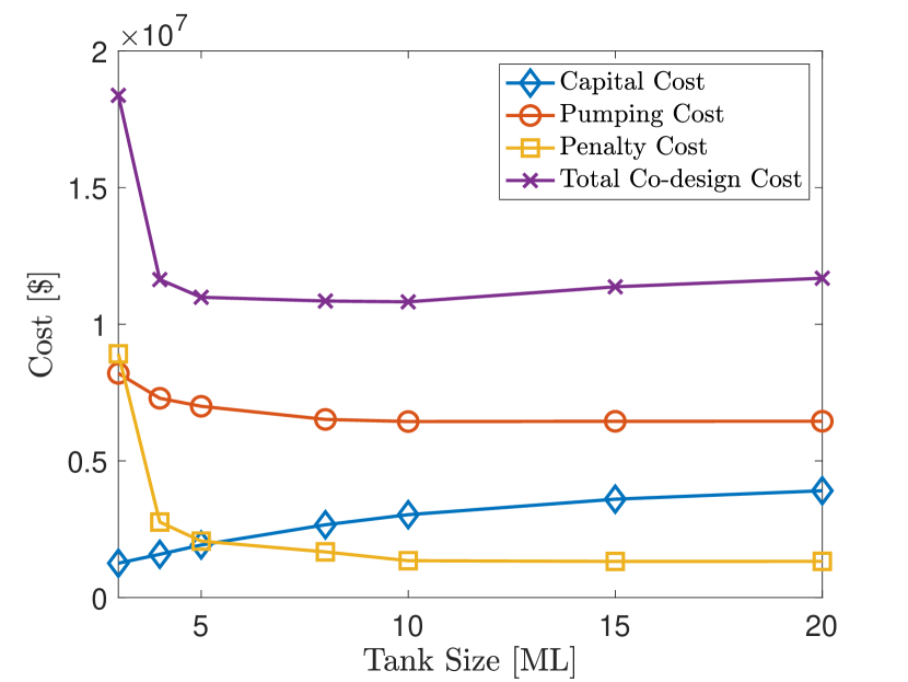
Figure 15: The cost comparison for a 50-year planning horizon with different tank sizes and optimal co-design control operations.

TABLE IV: Co-design computation results for the case study network.

Tank Size [ML]	Number of States	Capital Cost	Pumping Cost	Penalty Cost	Total Co-design Cost
3	20	$1,256,052	$8,202,120	$8,916,983	$18,375,154
4	26	$1,582,082	$7,291,233	$2,763,045	$11,636,360
5	33	$1,923,676	$6,999,010	$2,065,091	$10,987,777
8	52	$2,662,437	$6,517,730	$1,669,709	$10,849,875
10	65	$3,031,888	$6,440,382	$1,347,709	$10,819,979
15	97	$3,599,156	$6,449,178	$1,321,563	$11,369,897
20	130	$3,908,106	$6,451,298	$1,324,352	$11,683,756

V-C Comparison of Operations with Existing Infrastructure

The proposed co-design method can also be used to improve control operations for existing infrastructure, leveraging the optimal control parameters for a given tank size. Using historical data on water demands and electricity prices in 2019, we compared the co-design solutions and historical operations in 2019. The historical operation was based on trigger-level control. It should also be noted that our optimization considers 2019 data only, while SA Water strategy may have considered different metrics and risk scenarios over a longer time. Nevertheless the comparison is believed to serve as a reasonable representation of potential improvements to current practice. For this case study, the tank size is 38.5 ML, in which 28.5 ML is an emergency buffer. Moreover, the maximum volume of the existing storage is 136 ML. An EPANET hydraulic model of the case study was used in the closed-loop simulation. Table V shows the results.

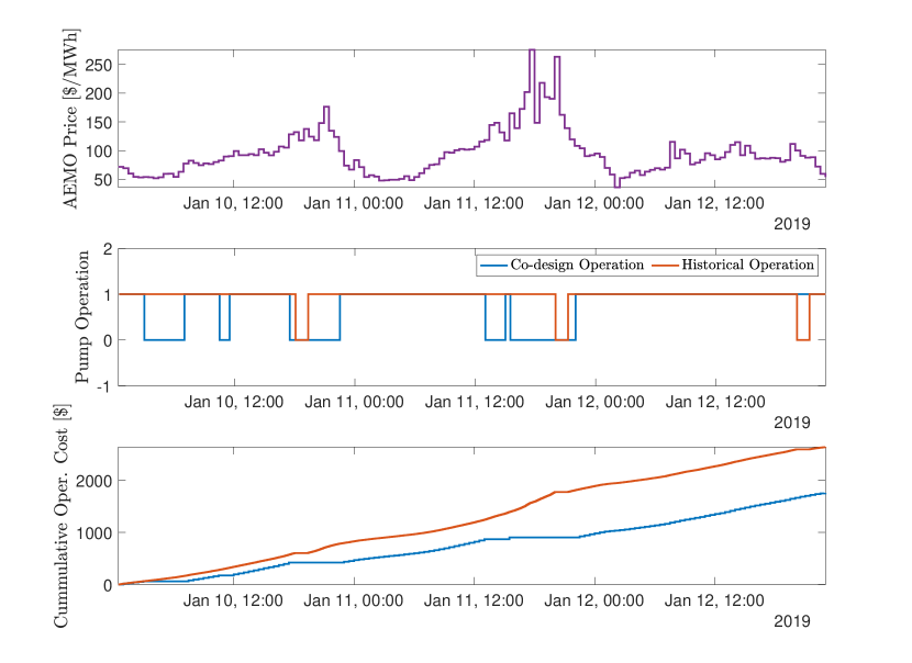
Figure 16: Comparison of operations in January 2019.

TABLE V: Comparison of historical operation and co-design operation by simulation for the year of 2019.

	Historical Operation		Co-design Operation
	Energy Cons. [kWh]	Energy Cost	Energy Cons. [kWh]	Energy Cost	Cost Saving	Percentage
Summer Months	1,305,914	$142,083	1,339,054	$123,436	-$18,647	-13%
Winter Months	622,756	$46,977	662,965	$31,102	-$15,875	-34%
Whole year	1,928,670	$189,060	2,002,019	$154,538	-$34,522	-18%

• Cost Savings = Energy Cost (Co-design Operation) - Energy Cost (Historical Operation),

• Percentage = Cost Saving/Energy Cost (Historical Operation).

During the summer period in 2019, the operation using the optimized price thresholds for the given tank size (referred as co-design operation) resulted in a 13% decrease in pumping cost relative to trigger-level operations, while a 34% decrease is observed during the winter months. Overall, the co-design solutions saved 18% in pumping costs for the year 2019. The considered control strategy based on the price threshold is hence effective and able to bring economic benefit to the operation of the existing water infrastructure.

VI Conclusions

In this paper, we have proposed a tractable stochastic co-design optimization method that simultaneously determines the optimal tank storage size and control parameters used in the considered control strategy. The co-design optimization is formulated based on asymptotic Markov chain theory and simplifying assumptions about the stochastic nature of electricity prices and water demands. We have also discussed the theoretical result on the convergence of long-run co-design cost to the expected on with probability 1. Through three examples and a real case study, we have illustrated and verified the effectiveness of the proposed co-design method.

Through the case study, it also shows that the co-design method cannot only be applied to situations where the infrastructure is going to be put in place. It also brings economic benefits to the operation of existing water infrastructure by finding the optimal price thresholds given the existing infrastructure.

As future research, the assumptions about the electricity prices and demands will be relaxed allowing for time dependencies that more accurately reflect the stochastic nature of actual electricity prices and water demands.

References

- [1] IEA, Electricity consumption in the water sector by process, 2014-2040. [Online]. Available: https://www.iea.org/data-and-statistics/charts/electricity-consumption-in-the-water-sector-by-process-2014-2040
- [2] D. A. Savic and G. A. Walters, “Genetic algorithms for least-cost design of water distribution networks,” Journal of water resources planning and management, vol. 123, no. 2, pp. 67–77, 1997.
- [3] J. Marques, M. Cunha, and D. Savić, “Many-objective optimization model for the flexible design of water distribution networks,” Journal of environmental management, vol. 226, pp. 308–319, 2018.
- [4] E. Batchabani and M. Fuamba, “Optimal tank design in water distribution networks: review of literature and perspectives,” Journal of water resources planning and management, vol. 140, no. 2, pp. 136–145, 2014.
- [5] W. Wu, H. R. Maier, and A. R. Simpson, “Multiobjective optimization of water distribution systems accounting for economic cost, hydraulic reliability, and greenhouse gas emissions,” Water Resources Research, vol. 49, no. 3, pp. 1211–1225, 2013.
- [6] G. Cembrano, G. Wells, J. Quevedo, R. Pérez, and R. Argelaguet, “Optimal control of a water distribution network in a supervisory control system,” Control engineering practice, vol. 8, no. 10, pp. 1177–1188, 2000.
- [7] Y. Wang, V. Puig, and G. Cembrano, “Non-linear economic model predictive control of water distribution networks,” Journal of Process Control, vol. 56, pp. 23–34, 2017.
- [8] V. Puig, C. Ocampo-Martínez, R. Pérez, G. Cembrano, J. Quevedo, and T. Escobet, Real-time monitoring and operational control of drinking-water systems. Springer, 2017.
- [9] Y. Guo, S. Wang, A. F. Taha, and T. H. Summers, “Optimal pump control for water distribution networks via data-based distributional robustness,” IEEE Transactions on Control Systems Technology, vol. 31, no. 1, pp. 114–129, 2023.
- [10] G. Zheng and Q. Huang, “Energy optimization study of rural deep well two-stage water supply pumping station,” IEEE Transactions on Control Systems Technology, vol. 24, no. 4, pp. 1308–1316, 2015.
- [11] Y. Wang, K. Too Yok, W. Wu, A. R. Simpson, E. Weyer, and C. Manzie, “Minimizing pumping energy cost in real-time operations of water distribution systems using economic model predictive control,” Journal of Water Resources Planning and Management, vol. 147, no. 7, p. 04021042, 2021.
- [12] H. Mala-Jetmarova, N. Sultanova, and D. Savic, “Lost in optimisation of water distribution systems? a literature review of system operation,” Environmental modelling & software, vol. 93, pp. 209–254, 2017.
- [13] A. K. Sampathirao, P. Sopasakis, A. Bemporad, and P. P. Patrinos, “Gpu-accelerated stochastic predictive control of drinking water networks,” IEEE Transactions on Control Systems Technology, vol. 26, no. 2, pp. 551–562, 2017.
- [14] M. Giuliani, J. D. Quinn, J. D. Herman, A. Castelletti, and P. M. Reed, “Scalable multiobjective control for large-scale water resources systems under uncertainty,” IEEE Transactions on Control Systems Technology, vol. 26, no. 4, pp. 1492–1499, 2017.
- [15] E. Creaco, A. Campisano, N. Fontana, G. Marini, P. Page, and T. Walski, “Real time control of water distribution networks: A state-of-the-art review,” Water research, vol. 161, pp. 517–530, 2019.
- [16] E. Salomons and M. Housh, “A practical optimization scheme for real-time operation of water distribution systems,” Journal of Water Resources Planning and Management, vol. 146, no. 4, p. 04020016, 2020.
- [17] K. Oikonomou and M. Parvania, “Optimal coordinated operation of interdependent power and water distribution systems,” IEEE Transactions on Smart Grid, vol. 11, no. 6, pp. 4784–4794, 2020.
- [18] F. Pecci, E. Abraham, and I. Stoianov, “Outer approximation methods for the solution of co-design optimisation problems in water distribution networks,” IFAC-PapersOnLine, vol. 50, no. 1, pp. 5373–5379, 2017.
- [19] M. Garcia-Sanz, “Control co-design: an engineering game changer,” Advanced Control for Applications: Engineering and Industrial Systems, vol. 1, no. 1, p. e18, 2019.
- [20] Y. Wang, E. Weyer, C. Manzie, and A. R. Simpson, “Co-design of control strategy and storage size for a water distribution system,” in 2022 IEEE Conference on Control Technology and Applications (CCTA), 2022, pp. 1440–1445.
- [21] S. P. Meyn and R. L. Tweedie, Markov chains and stochastic stability. Springer Science & Business Media, 2012.
- [22] A. N. Shiryaev, Probability, 2nd ed. Springer, 1996.
- [23] N. U. Prabhu, Stochastic Storage Processes: queues, insurance risk, and dams, and data communication. Springer Science & Business Media, 1998, no. 15.
- [24] D. P. Bertsekas and J. N. Tsitsiklis, Introduction to probability. Athena Scientific, 2008, vol. 1.
- [25] Y. Suhov and M. Kelbert, Probability and statistics by example: volume 2, Markov chains: a primer in random processes and their applications. Cambridge University Press, 2008, vol. 2.
- [26] J. C. Spall, Introduction to stochastic search and optimization: estimation, simulation, and control. John Wiley & Sons, 2005.
- [27] NEM Data, “Aggregated price and demand data in 2019,” (Accessed on 1/4/2022). [Online]. Available: https://aemo.com.au/energy-systems/electricity/national-electricity-market-nem/data-nem/aggregated-data
- [28] AEMO, Aggregated price and demand data, 2019. [Online]. Available: https://aemo.com.au/en/energy-systems/electricity/national-electricity-market-nem/data-nem/aggregated-data
- [29] Water Services Association of Australia, Water Supply Code of Australia: WSA 03-2011-3.1, Part 1: Planning and Design, 2011. [Online]. Available: https://www.wsaa.asn.au/shop/product/27046
- [30] NSW Office of Water, NSW Reference Rates Manual -Valuation of Water Supply, Sewerage and Stormwater Assets, 2014. [Online]. Available: https://nla.gov.au/nla.obj-3010354890/view