ALI-DPFL: Differentially Private Federated Learning with Adaptive Local Iterations

Abstract

Federated Learning (FL) is a distributed machine learning technique that allows model training among multiple devices or organizations by sharing training parameters instead of raw data. However, adversaries can still infer individual information through inference attacks (e.g. differential attacks) on these training parameters. As a result, Differential Privacy (DP) has been widely used in FL to prevent such attacks.

We consider differentially private federated learning in a resource-constrained scenario, where both privacy budget and communication round are constrained. By theoretically analyzing the convergence, we can find the optimal number of differentially private local iterations for clients between any two sequential global updates. Based on this, we design an algorithm of differentially private federated learning with adaptive local iterations (ALI-DPFL). We experiment our algorithm on the FashionMNIST and CIFAR10 datasets, and demonstrate significantly better performances than previous work in the resource-constraint scenario.

I Introduction

In federated learning, normally each client downloads the global model from the center sever, performs local iterations, and uploads the resulted training parameters back to the center sever. The center sever then updates the global model accordingly. The above steps repeat until the global model converges [1]. In this way, federated learning learns by communicating only training parameters other than raw data. Nevertheless, some studies have shown that federated learning still carries privacy risks. Training parameters, such as gradient values, can be used to recover a portion of the original data [2] or infer whether specific content originates from certain data contributors [3]. Melis et al. [4] also demonstrated that participants’ training data could be leaked by shared models. Therefore, additional measures need to be taken to protect data privacy in federated learning.

Many works[5, 6, 7, 8] have demonstrated that the technique of differential privacy (DP) could protect machine learning models from unintentional information leakage. In differentially private federated learning (DPFL), each client executes a certain number of local iterations with differential privacy before performing a global update. For each global update, DPFL consumes privacy budget according to the number of local iterations and communicates one round of training parameters, and thus DPFL should be constraint to both privacy budget and communication rounds. However, current DPFL schemes normally optimize the global model only with the constraint of limited privacy budget, overlooking the constraint of communication resources.

Existing DPFL schemes usually choose empirically a fixed number $\tau$ of local iterations for each global update, usually, $\tau=1$. They treat communication resource as unlimited, but in practice, it is often not the case. Communicating too much may incur great running time, and consume a large bandwidth. As shown in Figure 1, when both privacy budget $\epsilon$ and communication round count $R_{s}$ are limited, the optimal $\tau$ values to achieve the best accuracy are very different. It is also indicated that a fixed $\tau$ may fail to achieve satisfactory convergence performances [9][10][11]. Therefore, for the first time, in this paper we focus on finding a DPFL scheme with adaptive local iterations to achieve good performances when both privacy budget and communication round are constrained.

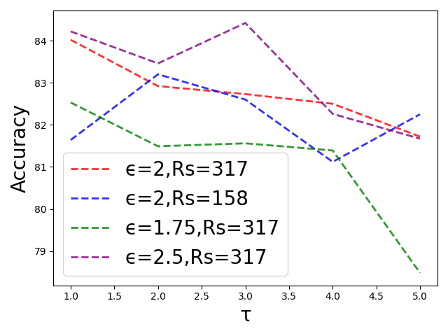
(a) FashionMNIST

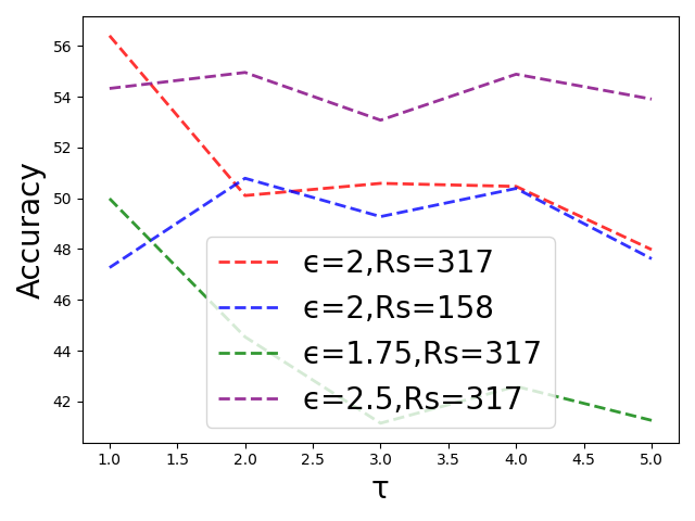
(b) CIFAR10

Figure 1: Performances of differentially private federated learning with different local iterations.

Through the convergence analysis, we derive a convergence bound related to the number $\tau$ of local iterations. Then, we propose a differentially private federated learning scheme with adaptive local iterations (ALI-DPFL), which searches in each communication round to find the optimal value ($\tau^{*}$) that minimizes the convergence bound. This value is then used as the number of local iterations in the next round, enabling the algorithm to converge quickly under the constraints of privacy budget and communication rounds, as shown in Figure 2. The main contributions of this paper are as follows:

1. We perform the convergence analysis of DPFL when privacy budget and comunication round are constrained, and establish a novel convergence bound concerning the number of local iterations.

2. Based on the convergence bound, we propose the ALI-DPFL algorithm, which uses adaptive local iterations to attain high accuracy and rapid convergence in the resource-constrained scenario.

3. We conduct extensive experiments to demonstrate that our approach outperforms the fixed $\tau$ strategy in the presence of Non-IID data distributions.

II Related Work

In previous research, many studies have provided proofs of convergence analysis for federated learning. Xiang Li et al. [12] demonstrated the convergence of the FedAvg algorithm in scenarios with Non-IID data and the possibility of device disconnections. Meanwhile, Tian Li et al. [10] analyzed the convergence of the FedProx algorithm in cases involving non-convex objective functions, Non-IID data, heterogeneous communication, and computational capabilities among devices. Furthermore, Kang Wei et al. [13] conducted convergence analysis on the NbAFL algorithm, they proposed to explore the relationship between convergence performance and privacy protection levels. Although these articles performed detailed work on convergence analysis, they primarily used it as a validation tool for algorithm correctness rather than utilizing the results for algorithm optimization.

In past studies, several works have combined differential privacy with federated learning. Kang Wei et al. [13] introduced the NbAFL algorithm, which first protects privacy in the uplink and then applies noise addition to both the uplink and downlink, achieving privacy protection. Xicong Shen et al.[14] proposed the PEDPFL algorithm by introducing a regularization term in the objective function, which mitigates the impact of noise introduced by differential privacy on the model. Additionally, Jie Fu et al.[15] proposed the Adap DP-FL algorithm, which adaptively clips gradients for different clients and rounds by adapting the added noise, optimizing the DPFL algorithm under Non-IID settings. However, the aforementioned works did not consider the impact of $\tau$ on the convergence speed of the algorithms.

Xiaosong Ma et al.[16] proposed the pFedLA algorithm, which introduced an adaptive hyper-network that applies layer-wise weighting to optimize personalized model aggregation under Non-IID settings. Tian Li et al. [10] generalized FedAvg by introducing a regularization term in the objective function and incorporating the variable $\gamma$ to control the regularization term and the number of epochs. However, these algorithms only focus on the federated learning and do not consider differential privacy.

To the best of our knowledge, this paper is the first work on convergence analysis and adaptive algorithms for DPFL in a resource-constrained scenario.

TABLE I: Summary of main notations

$F(\mathbf{w}$)	Global loss function
$F_{i}(\mathbf{w}$)	Local loss function for client $i$
$t$	Iteration index
$\mathbf{w}_{i}(t)$	Local model parameter at node $i$ at iteration $t$
$\hat{\mathbf{w}}(t)$	Global model parameter at iteration $t$
$\mathbf{w}^{*}$	True optimal model parameter that minimizes $F(\mathbf{\hat{\mathbf{w}}})$
$\eta$	Gradient descent step size
$\tau$	Number of local update iterations between two global aggregations
$T$	Total number of local iterations
$K$	Total number of global aggregation, equal to $T/\tau$
$R_{s}$	The number of communication rounds supported by communication resources
$R_{c}$	The number of communication rounds required by the privacy budget at $\tau=1$
$\rho$	Lipschitz parameter of $F_{i}(\mathbf{w})(\forall i)$ and $F(\mathbf{w})$
$\beta$	Smoothness parameter of $F_{i}(\mathbf{w})(\forall i)$ and $F(\mathbf{w})$
$\xi$	Gradient divergence
$h(\tau)$	Function defined in (10), gap between the model parameters obtained from distributed
$\varphi$	Constant defined in Theorem 2, control parameter
$G(\tau)$	Function defined in (13)
$\tau^{*}$	Optimal $\tau$ obtained by minimizing $G(\tau)$
$\sigma$	Standard deviation of Gaussian distribution
$d$	The dimension of model
$C$	Clipping norm
$B$	Batch size, equal to $|\mathcal{B}_{i}(t)|$
$||\cdot||$	$L_{2}$-norm

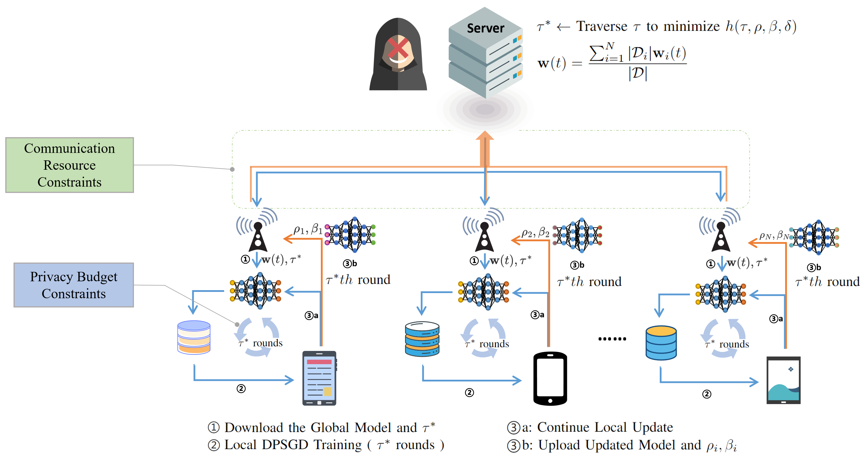
Figure 2: Adaptive Local Iterations Federated learning with differential privacy framework

III PRELIMINARIES

In this section, we will provide an overview of the background knowledge on FL and DP.

III-A Federated learning

A general FL system consisting of one server and $N$ clients. Each client, denoted as $\mathcal{C}_{i}$, holds a local database $\mathcal{D}_{i}$, where $i\in\{1,2,\dots,N\}$. $|\mathcal{D}_{i}|$ represent the size of dataset in Client $i$, and $|\mathcal{D}|=\sum_{i=1}^{N}|\mathcal{D}_{i}|$. The objective at the server is to learn a model using the data distributed across the $N$ clients. Each active client participating in the local training aims to find a vector $\mathbf{w}$ representing an neural network model that minimizes a specific loss function. The server then aggregates the weights received from the $N$ clients, which can be expressed as

$$\mathbf{w}(t)=\frac{\sum_{i=1}^{N}|\mathcal{D}_{i}|\mathbf{w}_{i}(t)}{|\mathcal{D}|}$$ (1)

where $\mathbf{w}_{i}(t)$ represents the parameter vector trained at the $i$-th client, $\mathbf{w}$ is the parameter vector after aggregation at the server, $t$ denotes the iteration (which may or may not include a global aggregation step), we consider the dataset size of each client to be consistent. The learning problem is to minimize $F(\mathbf{w})$, i.e., to find

$$\mathbf{w}^{*}\triangleq\arg\min F(\mathbf{w})$$ (2)

The function $F(\cdot)$ is defined as follows:

$$F(\mathbf{w})\triangleq\frac{\sum_{i=1}^{N}|\mathcal{D}_{i}|F_{i}(\mathbf{w})}{|\mathcal{D}|}$$ (3)

Here, $F_{i}(\cdot)$ represents the local loss function of the $i$-th client.

III-B Differential privacy

Differential privacy is a rigorous mathematical framework that formally defines the privacy loss of data analysis algorithms. Informally, it requires that any changes to a single data point in the training dataset can not cause statistically significant changes in the algorithm’s output.

Definition 1

(Differential Privacy[17]). A randomized mechanism $\mathcal{M}:\mathcal{X}\rightarrow\mathcal{R}$ provides ($\epsilon$, $\delta$)-DP, if for any two neighboring database $\mathcal{D}_{i},\mathcal{D}_{i}^{\prime}\in\mathcal{X}$ that differ in only a single entry, $\forall$ $\mathcal{S}$ $\subseteq$ Range($\mathcal{R}$),

$$\operatorname{Pr}\left[\mathcal{M}\left(\mathcal{D}_{i}\right)\in\mathcal{S}\right]\leq e^{\epsilon}\operatorname{Pr}\left[\mathcal{M}\left(\mathcal{D}_{i}^{\prime}\right)\in\mathcal{S}\right]+\delta$$ (4)

For numerical data, a Gaussian mechanism defined in [17] can be used to guarantee ($\epsilon$, $\delta$)-DP. According to [17], we present the following DP mechanism by adding artificial Gaussian noises.

III-C Differential Privacy Stochastic Gradient Descent

We introduce the traditional way of DPSGD in FL firstly. The local update in each iteration is performed on the parameter after possible global aggregation in the previous iteration. For each node $i$, the update rule is as follows:

$$\mathbf{w}_{i}(t)=\mathbf{w}_{i}(t-1)-\eta\nabla F_{i}\left(\mathbf{w}_{i}(t-1)\right)$$ (5)

Then, we add Gaussian noises $\mathcal{N}(0,\sigma^{2}C^{2}\mathbf{I}_{d})$ into each gradient, which should satisfy $(\epsilon,\delta)$-DP. For convenience, we rewrite the gradient $\nabla F_{i}(\hat{\mathbf{w}}_{i}(t))$ as $g_{i}(t)$:

1. $Clipping$: $\bar{g}_{i}(t)\leftarrow g_{i}(t)/\max(1,\frac{\|g_{i}(t)\|}{C})$

2. $Adding\ noise$: $\tilde{g}_{i}(t)\leftarrow\bar{g}_{i}(t)+\mathcal{N}(0,\sigma^{2}C^{2}\mathbf{I}_{d})$

3. $Gradient\ desent$:

   $$\hat{\mathbf{w}}_{i}(t+1)=\hat{\mathbf{w}}_{i}(t)-\eta\cdot\tilde{g}_{i}(t)$$ (6)

and average the $\hat{\mathbf{w}}_{i}(t)$ to get:

$$\hat{\mathbf{w}}(t)=\frac{\sum_{i=1}^{N}|\mathcal{D}_{i}|\hat{\mathbf{w}}_{i}(t-1)}{|\mathcal{D}|}$$ (7)

Input: loss function $F(\mathbf{w})$. Parameters: learning rate $\eta$, noise multiplier for training $\sigma$, local iterations $\tau$, clipping bound for training $C$

Output: the final trained model $\hat{\mathbf{w}}(K)$

1 Initialize $k=1$, $\mathbf{w}_{0}=\text{Initial()}$;

2 while $k<K$ do

3       for $i\in[1,2,\cdots,N]$  do

4             for $j\in[1,2,\cdots,\tau]$ do

5                   $t=(k-1)\tau+j$;

6                   Sample randomly a batch $\mathcal{B}_{i}(t)$ with probability $\frac{B}{|D_{i}|}$;

7                   for $s\in\mathcal{B}_{i}(t)$  do

8                         $g_{i}^{s}(t)\leftarrow\nabla F_{i}(\hat{\mathbf{w}_{i}}(t),s)$;

9                         $\bar{g}_{i}^{s}(t)\leftarrow g_{i}^{s}(t)/\max(1,\frac{\|g_{i}^{s}(t)\|}{C})$;

10                        

11                  $\widetilde{g}_{i}(t)\leftarrow\frac{1}{B}\left(\sum\limits_{s\in{\mathcal{B}_{i}(t)}}\bar{g}_{i}^{s}(t)+\mathcal{N}(0,\sigma^{2}{C}^{2}\mathbf{I}_{d})\right)$;

12                  

13                  $\hat{\mathbf{w}}_{i}(t+1)=\hat{\mathbf{w}}_{i}(t)-\eta\cdot\widetilde{g}_{i}(t)$;

14                  

15      $\text{Receive }\hat{\mathbf{w}}_{i}(k)$;

16       $k=k+1$;

17       $\hat{\mathbf{w}}(k)=\frac{\sum_{i=1}^{N}|\mathcal{D}_{i}|\hat{\mathbf{w}}_{i}(k-1)}{|\mathcal{D}|}$;

18       $\text{Broadcast }\hat{\mathbf{w}}(k)\text{ to each client}$ ;

19      

return $\hat{\mathbf{w}}(K)$

Algorithm 1 Differential Privacy Federated Learning

IV ALI-DPFL Algorithm

In this section, we propose our ALI-DPFL algorithm based on the findings from the convergence analysis. In Section IV-A, we conducted a convergence analysis of the traditional DPFL algorithm to explore the relationship between the convergence upper bound and $\tau$, resulting in equation (13). By minimizing equation (13), we can make $\hat{\mathbf{w}}(t)$ approach $\mathbf{w}^{*}$ more closely. The parameters $\rho$, $\beta$, and $\xi$ required in this equation can be computed during the model iterations. As shown in Fig 2, the algorithm in Section IV-B determines the number of local iterations $\tau^{*}$ for the next round of client updates by finding the minimum value of the convergence bound (13) through the traversal of different values of $\tau$. The key distinction between Algorithm 2 and Algorithm 1 is that the value of $\tau$ is dynamically determined by minimizing equation (13), rather than being fixed.

IV-A Motivation: Convergence Analysis of DPFL

In this subsection, we will analysis the convergence of traditional DPFL algorithm, as shown in Algorithm 1, and establishing a theoretical foundation for determining the optimal value of $\tau$ in each round.

We can divide the $T$ local iterations into $K$ different intervals, as shown in Figure 2, where only the first and last local iterations in each interval involve global aggregation. To denote the iteration interval $[(k-1)\tau,k\tau]$, we use the shorthand notation $[k]$, where $k=1,2,\dots,K$. For each interval $[k]$, we use $\hat{\mathbf{v}}_{[k]}(t)$ to denote an auxiliary parameter vector with noise that follows a centralized gradient descent.

Auxiliary parameter vector: The update rule is based on the global loss function $F(\mathbf{w})$, which is only observable when all data samples are available at a central location (called ”centralized gradient descent”). Here, $\mathbf{v}_{[k]}(t)$ is only defined for $t\in[(k-1)\tau,k\tau]$ for a given $k$. In contrast, the iteration in (6) is based on the local loss function $F_{i}(\mathbf{w})$.

At the beginning of each interval $[k]$, we define that $\hat{\mathbf{v}}_{[k]}(t)$ is ”synchronized” with $\hat{\mathbf{w}}(t)$, denoted as $\hat{\mathbf{v}}_{[k]}((k-1)\tau)\triangleq\hat{\mathbf{w}}((k-1)\tau)$. Here, $\hat{\mathbf{w}}(t)$ represents the average of local parameters defined in (7). It is important to note that $\hat{\mathbf{w}}_{i}((k-1)\tau)=\hat{\mathbf{w}}((k-1)\tau)$ holds for all $i$, as the global aggregation (or initialization when $k=1$) is performed in the iteration $(k-1)\tau$, the update of $\hat{\mathbf{v}}_{[k]}(t)$ show in below:

$$\hat{\mathbf{v}}_{[k]}(t)=\begin{cases}\hat{\mathbf{v}}_{[k]}(t-1)-\eta\cdot\tilde{g}_{[k]}(t-1),&t>k\tau\\ \hat{\mathbf{w}}(t),&t=k\tau\end{cases}$$ (8)

where

1. $g_{[k]}(t)\triangleq\nabla F(\hat{\mathbf{v}}_{[k]}(t))$

2. $\bar{g}_{[k]}(t)\leftarrow g_{[k]}(t)/\max(1,\frac{\|g_{[k]}(t)\|}{C})$

3. $\tilde{g}_{[k]}(t)\leftarrow\bar{g}_{[k]}(t)+\mathcal{N}(0,\sigma^{2}C^{2}\mathbf{I}_{d})$

The above definitions enable us to find the convergence bound of DPFL using a two-step approach. In the first step, we find the gap between $\hat{\mathbf{w}}\left(k\tau\right)$ and $\hat{\mathbf{v}}_{[k]}\left(k\tau\right)$ for each $k$. This gap is the difference between the distributed and centralized gradient descents after $\tau$ iterations of local updates without global aggregation. In the second step, we combine this gap with the convergence bound of $\hat{\mathbf{v}}_{[k]}(t)$ within each interval $[k]$ to obtain the convergence bound of $\hat{\mathbf{w}}(t)$.

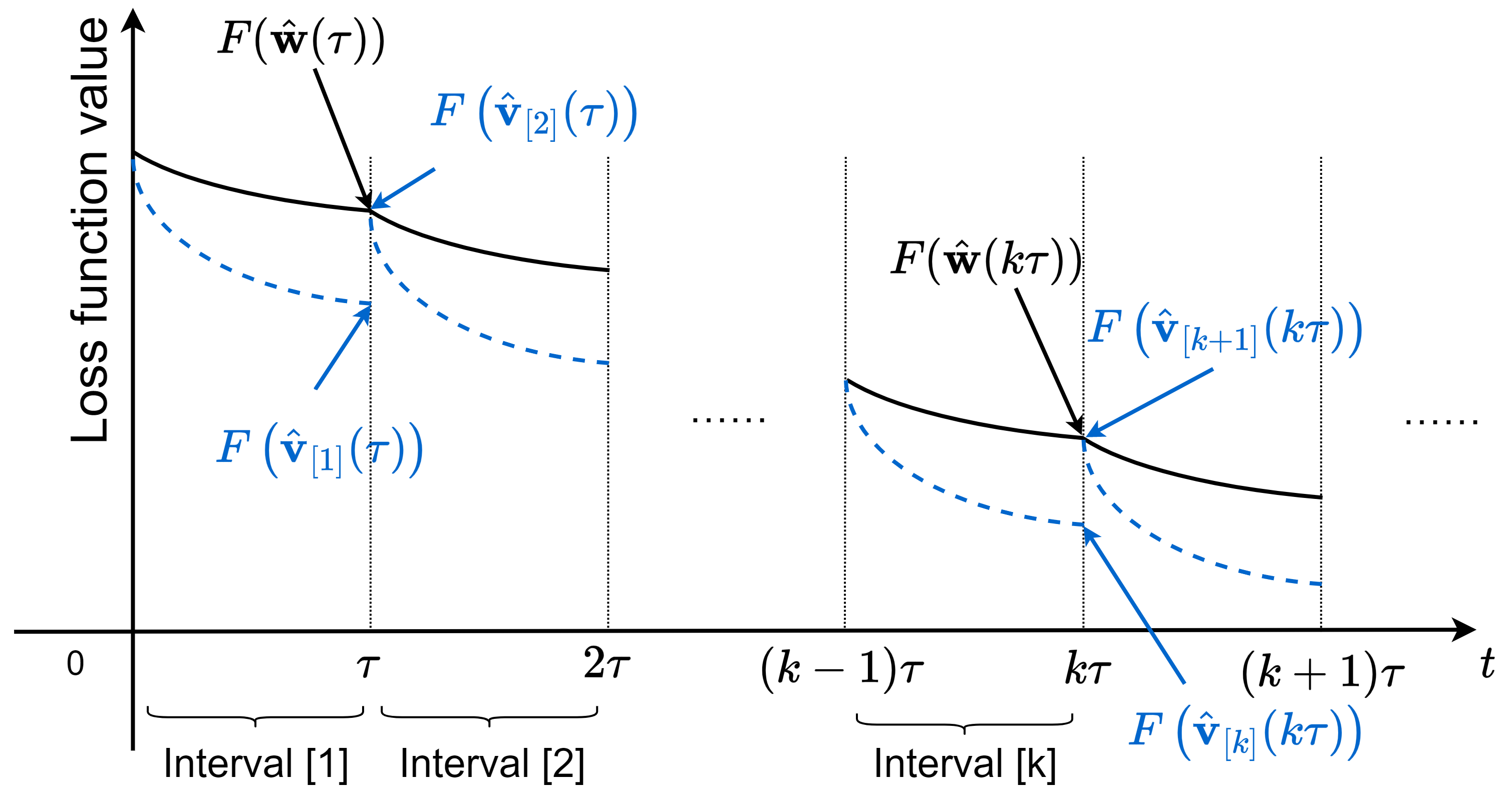
Figure 3: Illustration of definitions in different intervals.

For the purpose of the analysis, we make the following assumption to the loss function.

Assumption 1

We assume the following for all $i$:

1) $F_{i}(\mathbf{w})$ is convex

2) $F_{i}(\mathbf{w})$ is $\rho$-Lipschitz, i.e., $||F_{i}(\mathbf{w})-F_{i}(\mathbf{w}^{\prime})||\leq\rho||\mathbf{w}-\mathbf{w^{\prime}}||$ for any $\mathbf{w},\mathbf{w}^{\prime}$

3) $F_{i}(\mathbf{w})$ if $\beta$-smooth, i.e., $||\nabla F_{i}(\mathbf{w})-\nabla F_{i}(\mathbf{w}^{\prime})||\leq\beta||\mathbf{w}-\mathbf{w^{\prime}}||$ for any $\mathbf{w},\mathbf{w}^{\prime}$

4) there exists a clipping constant $C$ independent of $i,s$ such that $\|g_{i}^{s}(t)\|\leq C$

Lemma 1

$F(\mathbf{w})$ is convex,$\rho$-Lipschitz, and $\beta$-smooth Proof. Straight forwardly from Assumption 1, the definition of $F(\mathbf{w})$, and triangle inequality.

We also define the following metric to capture the divergence between the gradient of a local loss function and the gradient of the global loss function. This divergence is affected by how the data is distributed across different nodes.

Definition 2

For any $i$ and $\mathbf{w}$, we define $\xi_{i}$ as an upper bound of $||\nabla F_{i}(\mathbf{w})-\nabla F(\mathbf{w})||$, i.e.,

$$\left\|\nabla F_{i}(\mathbf{w})-\nabla F(\mathbf{w})\right\|\leq\xi_{i}$$ (9)

We also define $\xi\triangleq\frac{\sum_{i}D_{i}\xi_{i}}{D}$.

IV-A1 Main Result

The following theorem provides an upper bound on the difference between $\mathbf{w}(t)$ and $\mathbf{v}_{[k]}(t)$ when $t$ belongs to the interval $[k]$.

Theorem 1

For any interval $[k]$ and $t\in[k]$, we have

$$\mathbb{E}\left\|\hat{\mathbf{w}}(t)-\hat{\mathbf{v}}_{[k]}(t)\right\|\leqslant h(t-(k-1)\tau)$$ (10)

where

$$h(x)\triangleq\frac{\xi+\frac{2\sqrt{d}\sigma C}{B}}{\beta}\left((\eta\beta+1)^{x}-1\right)-\eta\cdot\frac{\xi+2\sqrt{d}\sigma C}{B}\cdot x$$ (11)

Furthermore, as $F(\cdot)$ is $\rho$-Lipschiz, we have $\mathbb{E}\|F\left(\hat{\mathbf{w}}(t)-F\left(\hat{\mathbf{v}}_{[k]}(t)\right)\|\leqslant\rho h(t-(k-1)\tau)\right.$.

Proof sketch. We begin by establishing an upper bound for $\mathbb{E}\|\hat{\mathbf{w}}_{i}(t)-\hat{\mathbf{v}}_{[k]}(t)\|$ for each node $i$ using mathematical induction. Based on this, we derive Equation (10). Please refer to Appendix A-Afor a detailed explanation.

It is worth noting that $\eta>0$ and $\beta>0$ always hold; otherwise, the gradient descent process or the loss function would become trivial. Consequently, applying the Bernoulli inequality, we have $(\eta\beta+1)^{x}\geq\eta\beta x+1$, where $x=0,1,2,\dots$. By substituting this inequality into Equation (11), we can confirm that $h(x)\geq 0$.

Moreover, it is evident that $h(0)=h(1)=0$. Thus, at the start of interval $[k]$, i.e., when $t=(k-1)\tau$, the upper bound in Equation (10) becomes zero. This aligns with the definition that $\hat{\mathbf{v}}_{[k]}((k-1)\tau)=\hat{\mathbf{w}}_{[k]}((k-1)\tau)$ for any $k$.

Theorem (1) provides an upper bound on the difference between distributed and centralized gradient descent, assuming that $\hat{\mathbf{v}}_{[k]}(t)$ in centralized gradient descent synchronizes with $\hat{\mathbf{w}}(t)$ at the beginning of each $[k]$. Based on this result, we first obtain the following theorem.

Theorem 2

When all the following conditions are satisfied:

1) $\eta\leq\frac{1}{\beta}$

2) $\eta\varphi-\frac{\rho h(\tau)}{\tau\lambda^{2}}>0$

3) $F(\hat{\mathbf{v}}_{[k]}\left(k\tau\right))-F(\mathbf{w}^{*})\geq\lambda$ for all $k$

4) $\lambda\leq F(\hat{\mathbf{w}}(T))-F(\mathbf{w}^{*})<1$

for some $\lambda>0$, where we define $\varphi\triangleq\omega(1-\frac{\beta\eta}{2})$, $\omega\triangleq\min_{k}\frac{1}{\|\hat{\mathbf{v}}_{[k]}((k-1)\tau)-\mathbf{w}^{*}\|}$, then the convergence upper bound after T iterations is given by:

$$\mathbb{E}(F(\hat{\mathbf{w}}(T))-F(\mathbf{w}^{*}))<\frac{1}{T\cdot(\eta\varphi-\frac{\rho h(\tau)}{\tau\lambda^{2}})}+\frac{\sqrt{3}}{3}$$ (12)

Proof sketch. We first analyze the convergence of $F(\hat{\mathbf{v}}_{[k]}(t))$ within each interval $[k]$. Then we combine this result with the gap between $F(\hat{\mathbf{w}}(t))$ and $F(\hat{\mathbf{v}}_{[k]}(t))$ from Theorem (1) to obtain the final result. For details, see Appendix A-B. We define the Right-Hand Side(RHS) of (12) as:

$$G(\tau)\triangleq\frac{1}{T\cdot(\eta\varphi-\frac{\rho h(\tau)}{\tau\lambda^{2}})}+\frac{\sqrt{3}}{3}$$ (13)

so that we can traverse the value of $\tau$ to optimize (13) to get $\tau^{*}$.

Both the broadcast of the model from the server to the clients and the uploading of the model from the clients to the server consume communication resources.

IV-B Our Algorithm

Our goal is to adjust the value of $\tau$ in order to minimize the (13). This allows $\hat{\mathbf{W}}(T)$ to approach $\mathbf{W}^{*}$ as closely as possible, thus achieving fast convergence in resource-constrained scenarios.

As depicted in Algorithm 2, the ALI-DPFL algorithm differs from the DPFL algorithm by adding the computation of values such as $\rho$, $\beta$, and $\xi$. Additionally, it requires the calculation of $\tau^{*}$, rather than utilizes a fixed $\tau$.

Input: loss function $F(\mathbf{w})$. Parameters: learning rate $\eta$, noise multiplier for training $\sigma$, batch size $B$, optimal local iterations $\tau^{*}$, clipping bound $C$, communication resources $C_{b}$, privacy budget $P_{b}$

Output: the final trained model $\hat{\mathbf{w}}(k)$

1 Initialize $k=1$, $t=0$, $\mathbf{w}_{0}=\text{Initial()}$, $\tau^{*}=1$, $p_{b}=0$, $c_{b}=0$;

2 while $c_{b}<C_{b}\And p_{b}<P_{b}$ do

3       for $i\in[1,2,\cdots,N]$  do

4             Estimate $\rho_{i}$, $\beta_{i}$ according to Assumption 1;

5             for $j\in[1,2,\cdots,\tau^{*}]$ do

6                   $t=t+1$;

7                   Sample randomly a batch $\mathcal{B}_{i}(t)$ with probability $\frac{B}{|D_{i}|}$;

8                   for $s\in\mathcal{B}_{i}(t)$  do

9                         $g_{i}^{s}(t)\leftarrow\nabla F_{i}(\hat{\mathbf{w}}_{i}(t),s)$;

10                         $\bar{g}_{i}^{s}(t)\leftarrow g_{i}^{s}(t)/\max(1,\frac{\|g_{i}^{s}(t)\|}{C})$;

11                        

12                  $\widetilde{g}_{i}(t)\leftarrow\frac{1}{B}\left(\sum\limits_{s\in{\mathcal{B}_{i}(t)}}\bar{g}_{i}^{s}(t)+\mathcal{N}(0,\sigma^{2}{C}^{2}\mathbf{I}_{d})\right)$;

13                  

14                  $\hat{\mathbf{w}}_{i}(t+1)=\hat{\mathbf{w}}_{i}(t)-\eta\cdot\widetilde{g}_{i}(t)$;

15                   Estimate privacy consumption $p$ and $p_{b}\leftarrow p_{b}+p$;

16                  

17      $\text{Receive }\hat{\mathbf{w}}_{i}(k),\rho_{i},\beta_{i}$;

18       $k=k+1$;

19       $\hat{\mathbf{w}}(k)=\frac{\sum_{i=1}^{N}|\mathcal{D}_{i}|\hat{\mathbf{w}}_{i}(k-1)}{|\mathcal{D}|}$;

20       Estimate $\xi_{i}$ according to some (9);

21       Weighted to get $\rho$, $\beta$, $\xi$;

22       Find $\tau^{*}$: Traverse $\tau$ to minimize (13) ;

23       $\text{Broadcast }\hat{\mathbf{w}}(k),\tau^{*}\text{ to each client}$ ;

24       Estimate communication consumption $r$ and $c_{b}\leftarrow c_{b}+r$

return $\hat{\mathbf{w}}(k)$

Algorithm 2 Adaptive Local Iterations Differential Privacy Federated Learning

• Client View: Among $N$ clients, we first receive $\hat{\mathbf{w}}(t)$ and $\tau^{*}$, then estimate the values of $\rho_{i}$ and $\beta_{i}$ to be returned to the server along with the model at the end of training. We perform $\tau^{*}$ iterations on each client. To eliminate the influence of batches on this algorithm, we set the number of batch to 1.

• Clipping and noise addition: In each batch, we perform per-sample gradient clipping, followed by averaging the gradients of the entire batch and adding noise.

• Server View: After receiving the models from each client, we average the weigh and use (9) to compute $\xi_{i}$ for each client. Then, we obtain the weighted values of $\rho$, $\beta$, and $\xi$, which will be used in the calculation of $\tau^{*}$.

• Perform Estimate: We estimate the values of $\rho$, $\beta$, and $\xi$ based on Assumption 1 and (9), as follows:

  $$\rho_{i} \leftarrow\frac{\|F_{i}(\hat{\mathbf{w}}_{i}(t))-F_{i}(\hat{\mathbf{w}}(t))\|}{\|\hat{\mathbf{w}}_{i}(t)-\hat{\mathbf{w}}(t)\|}$$

  $$\beta_{i} \leftarrow\frac{\|\nabla F_{i}(\hat{\mathbf{w}}_{i}(t))-\nabla F_{i}(\hat{\mathbf{w}}(t))\|}{\|\hat{\mathbf{w}}_{i}(t)-\hat{\mathbf{w}}(t)\|}$$

  $$\xi_{i} \leftarrow\|\nabla F_{i}(\hat{\mathbf{w}}(t))-\nabla F(\hat{\mathbf{w}}(t))\|$$

• Calculate the optimal number of local iterations $\tau^{*}$: We iterate over the values of $\tau$ in the range [1, $\tau_{m}$] to find the value of $\tau$ that minimizes (13), which becomes $\tau^{*}$. In our experiments, $\tau_{m}=\min\{2\tau^{*},100\}$.

V Privacy Analysis

Each client adds Gaussian noise satisfying differential privacy to the locally trained model can defend against the attacks mentioned in the threat model above. As a result, we only assess each client’s privacy loss from the perspective of a single client. Second, because each client’s locally trained pair of data samples has the same sampling rate and noise factor in each round, each client has the same privacy loss in each round. Following that, we examine the privacy budget for the $i$-th client (the privacy loss analysis for the other clients is the same as it is).

Theorem 3

(DP Privacy Loss of Algorithm 1). After $T$ local iterations, the $i$-th client DP Privacy budget of Algorithm 1 satisfies:

$$\begin{split}(\epsilon^{i}_{T},\delta)=(\sum_{t=0}^{T}\frac{1}{\alpha-1}\sum_{k=0}^{\alpha}\left(\begin{array}[]{l}\alpha\\ i\end{array}\right)(1-q)^{\alpha-k}q^{k}\\ \exp\left(\frac{k^{2}-k}{2\sigma^{2}}\right)+\frac{\log 1/\delta}{\alpha-1},\delta)\end{split}$$ (14)

where $q=\frac{B}{|D_{i}|}$ , $\sigma$ is noise scale and any integer $\alpha\geq 2$ .

$proof.$ We perform privacy loss calculation based on RDP[18]. We first use the sampling Gaussian theorem of RDP to calculate the privacy cost of each round, then we perform the advanced combination of RDP to combine the privacy cost of multiple rounds, and finally we convert the obtained to RDP privacy to DP.

Definition 3

(RDP privacy budget of SGM[19]). Let $SG_{q,\sigma}$, be the Sampled Gaussian Mechanism for some function $f$. If $f$ has sensitivity 1, $SG_{q,\sigma}$ satisfies $(\alpha,R)$-RDP whenever

$$R\leq\frac{1}{\alpha-1}\log max(A_{\alpha}(q,\sigma),B_{\alpha}(q,\sigma))$$ (15)

where

$$\left\{\begin{array}[]{l}A_{\alpha}(q,\sigma)\triangleq\mathbb{E}_{z\sim\mu_{0}}\left[\left(\mu(z)/\mu_{0}(z)\right)^{\alpha}\right]\\ B_{\alpha}(q,\sigma)\triangleq\mathbb{E}_{z\sim\mu}\left[\left(\mu_{0}(z)/\mu(z)\right)^{\alpha}\right]\end{array}\right.$$ (16)

with $\mu_{0}\triangleq\mathcal{N}\left(0,\sigma^{2}\right),\mu_{1}\triangleq\mathcal{N}\left(1,\sigma^{2}\right)\mbox{ and }\mu\triangleq(1-q)\mu_{0}+q\mu_{1}$

Further, it holds $\forall(q,\sigma)\in(0,1],\mathbb{R}^{+*},A_{\alpha}(q,\sigma)\geq B_{\alpha}(q,\sigma)$. Thus, $SG_{q,\sigma}satisfies\left(\alpha,\frac{1}{\alpha-1}\log\left(A_{\alpha}(q,\sigma)\right)\right)$-RDP .

Finally, [19] describes a procedure to compute $A_{\alpha}(q,\sigma)$ depending on integer $\alpha$.

$$A_{\alpha}=\sum_{k=0}^{\alpha}\left(\begin{array}[]{l}\alpha\\ k\end{array}\right)(1-q)^{\alpha-k}q^{k}\exp\left(\frac{k^{2}-k}{2\sigma^{2}}\right)$$ (17)

Definition 4

(Composition of RDP[18]). For two randomized mechanisms $f,g$ such that $f$ is $(\alpha,R_{1})$-RDP and $g$ is $(\alpha,R_{2})$-RDP the composition of $f$ and $g$ which is defined as $(X,Y)$(a sequence of results), where $X\sim f$ and $Y\sim g$, satisfies $(\alpha,R_{1}+R_{2})-RDP$

From Definition 3 and Definition 4, the following Lemma 2 is obtained.

Lemma 2

. Given the sampling rate $q=\frac{B}{|D_{i}|}$ for each round of the local dataset and $\sigma$ as the noise factor, the total RDP privacy loss of the i-th client for local iterations $T$ for any integer $\alpha\geq 2$ is:

$$\epsilon^{{}^{\prime}}(\alpha)_{T}^{i}=\sum_{t=0}^{T}\frac{1}{\alpha-1}\sum_{k=0}^{\alpha}\left(\begin{array}[]{l}\alpha\\ k\end{array}\right)(1-q)^{\alpha-i}q^{k}\exp\left(\frac{k^{2}-k}{2\sigma^{2}}\right)$$ (18)

Definition 5

(Translation from RDP to DP[18]). if a randomized mechanism $f:D\rightarrow\mathbb{R}$ satisfies $(\alpha,\epsilon)$-RDP ,then it satisfies$(\epsilon+\frac{\log 1/\delta}{\alpha-1},\delta)$-DP where $0<\delta<1$.

TABLE II: Condition I. Accuracy on $R_{s}\geq R_{c}$.

	$R_{s}=R_{c}$						$R_{s}=2R_{c}$
		F-MNIST			CIFAR10			F-MNIST			CIFAR10
$\epsilon=$	1.75	1.85	2	1.75	1.85	2	1.55	1.65	1.75	1.55	1.65	1.75
ALI-DPFL	82.02	83.88	84.19	46.32	53.01	56.76	80.57	81.86	82.58	39.82	44.12	50.14
$\tau=1$	81.94	83.71	84.02	46.27	52.90	56.41	79.98	81.84	82.53	39.33	44.06	49.99
$\tau=2$	81.48	82.84	82.92	42.91	47.34	50.11	79.66	79.88	81.49	32.55	38.63	44.54
$\tau=3$	81.26	82.61	82.73	41.33	45.98	50.59	78.55	77.51	81.56	31.23	37.20	41.14
$\tau=4$	79.17	82.44	82.50	40.84	44.03	50.47	78.37	77.90	81.39	28.96	33.24	42.59
$\tau=5$	79.64	80.46	81.72	42.06	45.32	47.98	77.68	76.96	78.48	26.38	38.02	41.25

TABLE III: Condition II. Accuracy on $R_{s}=\frac{1}{2}R_{c}$.

	F-MNIST			CIFAR10
$\epsilon=$	2	2.25	2.5	2	2.25	2.5
ALI-DPFL	83.44	83.58	83.25	51.92	53.86	55.17
$\tau=1$	81.64	82.96	83.39	47.27	52.66	54.33
$\tau=2$	83.20	81.94	83.46	50.79	53.41	54.96
$\tau=3$	82.60	82.99	83.24	49.28	52.04	53.08
$\tau=4$	81.12	83.54	82.26	50.39	52.41	54.89
$\tau=5$	82.25	77.96	81.67	47.62	52.63	53.91

TABLE IV: Condition II. Accuracy on $R_{s}=\frac{1}{5}R_{c}$.

	F-MNIST			CIFAR10
$\epsilon=$	2.75	3.25	3.75	2.75	3.25	3.75
ALI-DPFL	84.07	84.31	84.58	55.54	55.67	57.25
$\tau=1$	82.14	81.99	83.70	47.20	51.00	53.37
$\tau=3$	83.60	83.57	83.75	52.85	55.60	56.84
$\tau=5$	82.45	80.70	81.72	55.14	55.17	55.21
$\tau=7$	82.29	81.16	82.87	54.30	53.94	55.42
$\tau=9$	80.78	71.13	81.36	52.92	52.80	54.76

By Lemma 2 and Definition 5, Theorem 3 is proved. In practice, given $\sigma$, $\delta$ and $q$ at each round, we select $\alpha$ from $\left\{2,3,...,64\right\}$ and determine the smallest $\epsilon_{*}$ in Theorem 1. The privacy loss is the pair $(\epsilon_{*},\delta)$.

VI EXPERIMENT

We conducted a series of comparative experiments on the FashionMnist and CIFAR10 datasets. The experiment results demonstrate that our ALI-DPFL algorithm can achieve excellent performance and improve accuracy under different ratios between communication resources and privacy budget resources.

VI-A Initialize

In our experiments, we suppose 10 clients and adopt the similar methodology as MHR et al. [20] for Non-IID partitioning of data to each client. We conduct our experiments under the following two real datasets:

FashionMNIST: FashionMNIST is a widely used image classification dataset with grayscale images of fashion items in 10 categories. It has 60,000 training samples and 10,000 testing samples, each with a size of 28×28 pixels.

CIFAR10: The CIFAR10 dataset consists of images belonging to 10 categories. Each category contains 6,000 image samples, resulting in a total of 50,000 training samples and 10,000 testing samples. The images in the dataset have a size of 32×32 pixels and contain RGB (red, green, blue) color channels.

Parameter settings: For FashionMNIST and CIFAR10, we employ the DPSGD optimizer with a base learning rate of 0.5. Additionally, we set the batch size $B$=75, noise scale $\sigma$=1.1 and cipping bound $C$=0.1.

VI-B Performance

In Equation (11), we mentioned that $\tau=1$ can make $h(x)=0$, and the convergence bound of Equation (12) is minimized. Therefore, when the number of communication rounds supported by communication resources (denoted by $R_{s}$, ”Resource of Server”) is greater than or equal to the number of communication rounds required by the privacy budget at $\tau=1$ (denoted by $R_{c}$, ”Resource of Client”), $\tau=1$ is the optimal choice. In previous convergence analysis works that focus on the relationship between accuracy and the number of local iterations [12][21][22][23], we observed their convergence bounds, finding that accuracy and the number of local iterations always appear simultaneously in the denominator, when the accuracy is fixed, the larger the number of iterations, the smaller the convergence bound. And when the total amount of resources is fixed, $\tau=1$ can maximize the number of iterations, which aligns with our viewpoint. Based on this observation, we conducted experimental design:

$\textit{Condition I}:$ When $R_{s}\geq R_{c}$, according to the analysis above, setting all values in the $\tau$-list to 1 can achieve optimal model performance. Therefore, we validate the cases of $R_{s}=R_{c}$ and $R_{s}=2R_{c}$ under three fixed $R_{s}$ conditions, and the experimental results are shown in TABLE II.

$\textit{Condition II}:$ When $R_{s}<R_{c}$, setting values in the $\tau$-list to 1 can not fully utilize local resources. Therefore, we validate the cases of $R_{s}=\frac{1}{2}R_{c}$ and $R_{s}=\frac{1}{5}R_{c}$ under three fixed $R_{s}$ conditions, and the experimental results are shown in TABLE III and IV.

In our experiment, we compared the ALI-DPFL method with the fixed $\tau$ method, and conducted experimental comparisons for four different ratios: $R_{s}=R_{c}$, $R_{s}=2R_{c}$, $R_{s}=\frac{1}{2}R_{c}$, and $R_{s}=\frac{1}{5}R_{c}$, under three conditions: $R_{s}=\{158,231,317\}$. To accommodate the four cases of $R_{s}=\mathrm{n}\cdot R_{c}$ and the three values of $R_{s}=\{158,231,317\}$, we choose the following privacy budget $\epsilon=\{1.55,1.65,1.75,1.85,2,2.25,2.5,2.75,3.25,3.75\}$ to support $\{79,122,177,231,317,457,598,775,1123,1585\}$ iterations, which can approximately meet the experimental requirements.

On the FashionMNIST and CIFAR10 datasets, when $R_{s}\geq R_{c}$, the $\tau$ list of ALI-DPFL is all 1, training models with $\tau^{*}=1$ yields the highest accuracy, which is consistent with our analysis. When $R_{s}<R_{c}$, the $\tau$ list is shown in Figure 6, and in most cases, the ALI-DPFL algorithm achieves higher accuracy than any fixed $\tau$ algorithm.

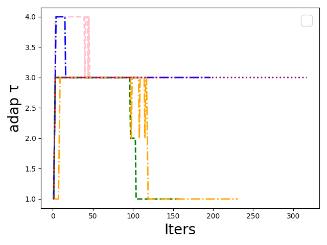
Figure 4: $\tau$ list in FashionMNIST dataset.

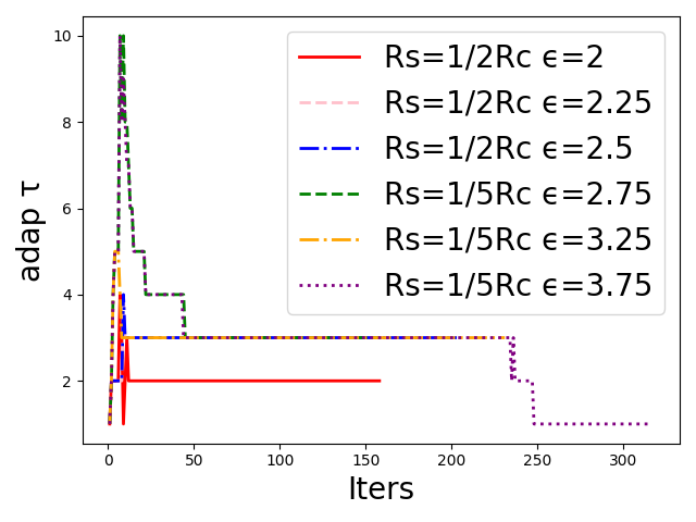
Figure 5: $\tau$ list in CIFAR10 dataset.

Figure 6: Adaptive $\tau$ value in different datasets.

VII CONCLUSION

In this paper, we present an algorithm of Differentially Private Federated Learning with Adaptive Local Iterations (ALI-DPFL), in the scenario where privacy budget and communication round are constrained. Through a theoretical convergence analysis of DPFL, we derive a convergence bound depending on the number $\tau$ of local iterations, and improve the performance of federated learning by finding the optimal $\tau$. We formally prove the privacy of the proposed algorithm with the RDP technique, and conduct extensive experiments to demonstrate that ALI-DPFL significantly outperforms existent schemes in the resource-constraint scenario.

Appendix A Appendix

A-A Proof of Theorem 1

To prove Theorem 1, we first introduce the following lemma.

Lemma 3

Referring to C.1 in [24], we have:

$$\mathbb{E}\left[\|\tilde{g}_{i}(t)-g_{i}(t)\|\right]\leq\frac{2\sqrt{d}\sigma C}{B}$$ (19)

Lemma 4

For any interval $[k]$, and $t\in[(k-1)\tau,k\tau)$, we have

$$\mathbb{E}\|\hat{\mathbf{w}}_{i}(t)-\hat{\mathbf{v}}_{[k]}(t)\|\leqslant g_{i}(t-(k-1)\tau)$$ (20)

where we define the function $g_{i}(x)$ as:

$$g_{i}(x)\triangleq\frac{\xi_{i}+\frac{2\sqrt{d}\sigma C}{B}}{\beta}((\eta\beta+1)^{x}-1)$$

Proof. We prove it by mathematical induction.

Step 1. When $x=t-(k-1)\tau=0$, i.e., $t=(k-1)\tau$, which corresponds to a communication step, we have the following conditions:

1. $\hat{\mathbf{w}}((k-1)\tau)=\hat{\mathbf{v}}_{[k]}((k-1)\tau)$,

2. $\hat{\mathbf{w}}((k-1)\tau)=\hat{\mathbf{w}}_{i}((k-1)\tau)$,

which can simply get $\hat{\mathbf{w}}_{i}((k-1)\tau)=\hat{\mathbf{v}}_{[k]}((k-1)\tau)$.

Thus, we can simplify the expressions as follows:

$$\mathbb{E}\|\hat{\mathbf{w}}_{i}((k-1)\tau)-\hat{\mathbf{v}}_{[k]}((k-1)\tau)\|=0$$

$$=\frac{\xi_{i}+\frac{2\sqrt{d}\sigma C}{B}}{\beta}((\eta\beta+1)^{0}-1)=g_{i}(0)$$

Therefore, (20) holds when $x=0$.

Step 2. Let us assume that (20) holds when $x=a$, i.e., $t=a+(k-1)\tau$, then there is

$$\mathbb{E}\|\hat{\mathbf{w}}_{i}(a+(k-1)\tau)-\hat{\mathbf{v}}_{[k]}(a+(k-1)\tau)\|$$

$$\leqslant g_{i}(a)=\frac{\xi_{i}+\frac{2\sqrt{d}\sigma C}{B}}{\beta}((\eta\beta+1)^{a}-1)$$

Step 3. When $x=a+1$, i.e. $t=a+1+(k-1)\tau$, we have:

$$\left\|\hat{\mathbf{w}}_{i}(a+1+(k-1)\tau)-\hat{\mathbf{v}}_{[k]}(a+1+(k-1)\tau)\right\|$$

$$\leqslant\left\|\hat{\mathbf{w}}_{i}(a+(k-1)\tau)-\hat{\mathbf{v}}_{[k]}(a+(k-1)\tau)\right\|$$

$$\quad+\eta\left\|\tilde{g}_{i}(a)-\tilde{g}_{[k]}(a)\right\|$$

$$=\left\|\hat{\mathbf{w}}_{i}(a+(k-1)\tau)-\hat{\mathbf{v}}_{[k]}(a+(k-1)\tau)\right\|$$

$$\quad+\eta\|\tilde{g}_{i}(a)-{g}_{i}(a)+{g}_{i}(a)-\tilde{g}_{[k]}(a)\|$$

Here we take expectation

$$\mathbb{E}\left\|\hat{\mathbf{w}}_{i}(a+1+(k-1)\tau)-\hat{\mathbf{v}}_{[k]}(a+1+(k-1)\tau)\right\|$$

$$\leq\mathbb{E}\left\|\hat{\mathbf{w}}_{i}(a+(k-1)\tau)-\hat{\mathbf{v}}_{[k]}(a+(k-1)\tau)\right\|+\eta\cdot\frac{2\sqrt{d}\sigma C}{B}$$

$$\quad+\eta\cdot\mathbb{E}\|\nabla F_{i}(\hat{\mathbf{w}}_{i}(a+(k-1)\tau))-\nabla F(\hat{\mathbf{v}}_{[k]}(a+(k-1)\tau))\|$$

Where we use triangle inequality and (19)

$$=\mathbb{E}\left\|\hat{\mathbf{w}}_{i}(a+(k-1)\tau)-\hat{\mathbf{v}}_{[k]}(a+(k-1)\tau)\right\|+\eta\cdot\frac{2\sqrt{d}\sigma C}{B}$$

$$\quad+\eta\cdot\mathbb{E}\|\nabla F_{i}(\hat{\mathbf{w}}_{i}(a+(k-1)\tau))-\nabla F_{i}(\hat{\mathbf{v}}_{[k]}(a+(k-1)\tau))$$

$$\quad+\nabla F_{i}(\hat{\mathbf{v}}_{[k]}(a+(k-1)\tau))-\nabla F(\hat{\mathbf{v}}_{[k]}(a+(k-1)\tau))\|$$

Where we add zero term

$$\leq\mathbb{E}\left\|\hat{\mathbf{w}}_{i}(a+(k-1)\tau)-\hat{\mathbf{v}}_{[k]}(a+(k-1)\tau)\right\|+\eta\cdot\frac{2\sqrt{d}\sigma C}{B}$$

$$\quad+\eta\beta\mathbb{E}\left\|\hat{\mathbf{w}}_{i}(a+(k-1)\tau)-\hat{\mathbf{v}}_{[k]}(a+(k-1)\tau)\right\|+\eta\xi_{i}$$

Where we use $$\beta$$-smooth, triangle inequality and (9)

$$\leq(1+\eta\beta)g_{i}(a+(k+1)\tau)+\eta\left(\frac{2\sqrt{d}\sigma C}{B}+\xi_{i}\right)$$

Where we use step 2.

$$=(1+\eta\beta)\frac{\xi_{i}+\frac{2\sqrt{d}\sigma C}{B}}{\beta}((\eta\beta+1)^{a}-1)+\eta\left(\frac{2\sqrt{d}\sigma C}{B}+\xi_{i}\right)$$

$$=\frac{\xi_{i}+\frac{2\sqrt{d}\sigma C}{B}}{\beta}((\eta\beta+1)^{a+1}-1)$$

Therefore, (20) holds when $x=a+1$.

Summing up, with the completion of mathematical induction, (20) holds.

Proof of Theorem 1. From (6) and (7), we have:

$$\hat{\mathbf{w}}(t)=\hat{\mathbf{w}}(t-1)-\eta\frac{\sum_{i}D_{i}\tilde{g}_{i}(t-1)}{D}$$ (21)

Then, for $t\in((k-1)\tau,k\tau]$, we have:

$$\|\hat{\mathbf{w}}(t)-\hat{\mathbf{v}}_{[k]}(t)\|$$

$$=\|\hat{\mathbf{w}}(t-1)-\eta\frac{\sum_{i}D_{i}\tilde{g}_{i}(t-1))}{D}-\hat{\mathbf{v}}_{[k]}(t-1)+\eta\tilde{g}_{[k]}(t-1)\|$$

$$\leqslant\|\hat{\mathbf{w}}(t-1)-\hat{\mathbf{v}}_{[k]}(t-1)\|$$

$$\quad+\eta\frac{\sum_{i}D_{i}(\|\tilde{g}_{i}(t-1)-\tilde{g}_{[k]}(t-1)\|)}{D}$$

Where use triangle inequality

$$\leqslant\|\hat{\mathbf{w}}(t-1)-\hat{\mathbf{v}}_{[k]}(t-1)\|$$

$$\quad+\eta\frac{\sum_{i}D_{i}(\beta\|\hat{\mathbf{w}}_{i}(t-1)-\hat{\mathbf{v}}_{[k]}(t-1)\|)}{D}$$

Where use the $$\beta$$-smooth

Expect both sides of inequality:

$$\mathbb{E}\|\hat{\mathbf{w}}(t)-\hat{\mathbf{v}}_{[k]}(t)\|-\mathbb{E}\|\hat{\mathbf{w}}(t-1)-\hat{\mathbf{v}}_{[k]}(t-1)\|$$

$$\leqslant\eta\frac{\sum_{i}D_{i}(\beta\mathbb{E}\|\hat{\mathbf{w}}_{i}(t-1)-\hat{\mathbf{v}}_{[k]}(t-1)\|)}{D}$$

$$\leqslant\eta\frac{\sum_{i}D_{i}\left(\beta g_{i}(t-(k-1)\tau-1)\right)}{D}$$

Where use the (20)

$$=\eta\beta\frac{\sum_{i}D_{i}}{D}\left(\frac{\xi_{i}+\frac{2\sqrt{d}\sigma C}{B}}{\beta}\left((\eta\beta+1)^{t-(k-1)\tau-1}-1\right)\right)$$

$$=\eta\cdot\left(\xi+\frac{2\sqrt{d}\sigma C}{B}\right)\left((\eta\beta+1)^{t-(k-1)\tau-1}-1\right)$$

Thus, we have:

$$\mathbb{E}\|\hat{\mathbf{w}}(t)-\hat{\mathbf{v}}_{[k]}(t)\|-\mathbb{E}\|\hat{\mathbf{w}}(t-1)-\hat{\mathbf{v}}_{[k]}(t-1)\|$$

$$\leqslant\eta\cdot\left(\xi+\frac{2\sqrt{d}\sigma C}{B}\right)\left((\eta\beta+1)^{t-(k-1)\tau-1}-1\right)$$

Now, let’s $\displaystyle\sum_{y=(k-1)\tau+1}^{t}$ the left of (A-A):

$$\displaystyle\sum_{y=(k-1)\tau+1}^{t}(\mathbb{E}\|\hat{\mathbf{w}}(t)-\hat{\mathbf{v}}_{[k]}(t)\|-\mathbb{E}\|\hat{\mathbf{w}}(t-1)-\hat{\mathbf{v}}_{[k]}(t-1)\|)$$

$$=\mathbb{E}\|\hat{\mathbf{w}}((k-1)\tau+1)-\hat{\mathbf{v}}_{[k]}((k-1)\tau+1)\|$$

$$\quad-\mathbb{E}\|\hat{\mathbf{w}}((k-1)\tau)-\hat{\mathbf{v}}_{[k]}((k-1)\tau)\|$$

$$\quad+\mathbb{E}\|\hat{\mathbf{w}}((k-1)\tau+2)-\hat{\mathbf{v}}_{[k]}((k-1)\tau+2)\|$$

$$\quad-\mathbb{E}\|\hat{\mathbf{w}}((k-1)\tau+1)-\hat{\mathbf{v}}_{[k]}((k-1)\tau+1)\|$$

$$\quad+\cdots$$

$$\quad+\mathbb{E}\|\hat{\mathbf{w}}(t)-\hat{\mathbf{v}}_{[k]}(t)\|$$

$$\quad-\mathbb{E}\|\hat{\mathbf{w}}(t-1)-\hat{\mathbf{v}}_{[k]}(t-1)\|$$

$$=\mathbb{E}\|\hat{\mathbf{w}}(t)-\hat{\mathbf{v}}_{[k]}(t)\|-\mathbb{E}\|\hat{\mathbf{w}}((k-1)\tau)-\hat{\mathbf{v}}_{[k]}((k-1)\tau)\|$$

$$=\mathbb{E}\|\hat{\mathbf{w}}(t)-\hat{\mathbf{v}}_{[k]}(t)\|$$

Where from the definition $$\hat{\mathbf{w}}((k-1)\tau)\triangleq\hat{\mathbf{v}}_{[k]}((k-1)\tau)$$

Follow on, let’s $\displaystyle\sum_{y=(k-1)\tau+1}^{t}$ the right of (A-A):

$$\displaystyle\sum_{y=(k-1)\tau+1}^{t}\left(\eta\left(\xi+\frac{2\sqrt{d}\sigma C}{B}\right)((\eta\beta+1)^{t-(k-1)\tau-1}-1)\right)$$

$$=\displaystyle\sum_{z=1}^{t-(k-1)\tau}\left(\eta(\xi+\frac{2\sqrt{d}\sigma C}{B})(\eta\beta+1)^{z-1}-\eta(\frac{2\sqrt{d}\sigma C}{B}+\xi)\right)$$

(exchange element $$z=y-(k-1)\tau$$)

$$=\frac{\xi+\frac{2\sqrt{d}\sigma C}{B}}{\beta}\left((\eta\beta+1)^{t-(k-1)\tau}-1\right)$$

$$\quad-\eta(\frac{\xi+2\sqrt{d}\sigma C}{B})\left(t-(k-1)\tau\right)$$

$$=h\left(t-(k-1)\tau\right)$$

Above all, we have:

$$\mathbb{E}\|\hat{\mathbf{w}}(t)-\hat{\mathbf{v}}_{[k]}(t)\|\leqslant h\left(t-(k-1)\tau\right)$$ (23)

where:

$$h(x)\triangleq\frac{\xi+\frac{2\sqrt{d}\sigma C}{B}}{\beta}\left((\eta\beta+1)^{x}-1\right)-\eta(\frac{\xi+2\sqrt{d}\sigma C}{B})x$$ (24)

Furthermore, as $F(\cdot)$ is $\rho$-Lipschiz, we have

$$\mathbb{E}\|F\left(\hat{\mathbf{w}}(t)-F\left(\hat{\mathbf{v}}_{[k]}(t)\right)\|\leqslant\rho h(t-(k-1)\tau)\right.$$ (25)

So far, we have proved the Theorem 1.

A-B Proof of Theorem 2

To prove Theorem 2, we first introduce some additional definitions and lemmas.

Definition 6

For an interval [k], we define $\theta_{[k]}(t)=F(\hat{\mathbf{v}}_{[k]}(t))-F(\mathbf{w}^{*})$, for a fixed $k$, $t$ is defined between $(k-1)\tau\leq t\leq k\tau$.

According to the convergence lower bound of gradient descent given in Theorem 3.14 of [25], we always have

$$\theta_{[k]}(t)>0$$ (26)

for any finite $t$ and $k$.

Lemma 5

When $\eta\leqslant\frac{1}{\beta}$, for any $k$, and $t\in[(k-1)\tau,k\tau]$, we have that $\|\hat{\mathbf{v}}_{[k]}(t)-\mathbf{w}^{*}\|$ does not increase with t, where $\mathbf{w}^{*}$ is the optimal parameter defined in (2).
Proof.

$$\left\|\hat{\mathbf{v}}_{[k]}(t+1)-\mathbf{w}^{*}\right\|^{2}$$

$$=\left\|(\hat{\mathbf{v}}_{[k]}(t)-\mathbf{w}^{*})-\eta\tilde{g}_{[k]}(t)\right\|^{2}$$

$$=\left\|\hat{\mathbf{v}}_{[k]}(t)-\mathbf{w}^{*}\right\|^{2}-2\eta(\tilde{g}_{[k]}(t))^{\mathrm{T}}\left(\hat{\mathbf{v}}_{[k]}(t)-\mathbf{w}^{*}\right)$$

$$\quad+\eta^{2}\left\|\tilde{g}_{[k]}(t)\right\|^{2}$$

Because $F$ is $\beta$-smooth, from (26) and Lemma 3.5 of [25], we have

$$0<\theta_{[k]}(t)\leqslant\left(\tilde{g}_{[k]}(t)\right)^{\mathrm{T}}\left(\hat{\mathbf{v}}_{[k]}(t)-\mathbf{w}^{*}\right)-\frac{\|\tilde{g}_{[k]}(t)\|^{2}}{2\beta}$$

Therefore,

$$\left\|\hat{\mathbf{v}}_{[k]}(t+1)-\mathbf{w}^{*}\right\|^{2}$$

$$<\left\|\hat{\mathbf{v}}_{[k]}(t)-\mathbf{w}^{*}\right\|^{2}-\eta(\frac{1}{\beta}-\eta)\|\tilde{g}_{[k]}(t)\|^{2}$$

$$\leqslant\left\|\hat{\mathbf{v}}_{[k]}(t)-\mathbf{w}^{*}\right\|^{2}$$

(since $$\eta\leqslant\frac{1}{\beta}$$)

Lemma 6

For any $k$, when $\eta\leqslant\frac{1}{\beta}$ and $t\in[(k-1)\tau,k\tau)$, we have

$$F(\hat{\mathbf{v}}_{[k]}(t+1))-F(\hat{\mathbf{v}}_{[k]}(t)) \leqslant\eta(\frac{\beta\eta}{2}-1)\left\|\tilde{g}_{[k]}(t)\right\|^{2}$$ (27)

Proof.

Because $F$ is $\beta$-smooth, from Lemma 3.4 of [25], we have

$$F(\mathbf{x})\leqslant F(\mathbf{y})+\nabla F(\mathbf{y})^{T}(\mathbf{x}-\mathbf{y})+\frac{\beta}{2}\|\mathbf{x}-\mathbf{y}\|^{2}$$

for arbitrary $\mathbf{x}$ and $\mathbf{y}$. Thus,

$$F(\hat{\mathbf{v}}_{[k]}(t+1))-F(\hat{\mathbf{v}}_{[k]}(t))$$

$$\leqslant\tilde{g}_{[k]}(t)^{T}(\hat{\mathbf{v}}_{[k]}(t+1)-\hat{\mathbf{v}}_{[k]}(t))+\frac{\beta}{2}\|\hat{\mathbf{v}}_{[k]}(t+1)-\hat{\mathbf{v}}_{[k]}(t)\|^{2}$$

$$\leqslant-\eta\tilde{g}_{[k]}(t)^{T}\tilde{g}_{[k]}(t)+\frac{\beta\eta^{2}}{2}\|\tilde{g}_{[k]}(t)\|^{2}$$

(both from gradient decent (8))

$$\leqslant\eta(\frac{\beta\eta}{2}-1)\left\|\tilde{g}_{[k]}(t)\right\|^{2}$$

Lemma 7

For any k, when $\eta\leq\frac{1}{\beta}$ and $t\in[(k-1)\tau,k\tau)$, we have

$$\frac{1}{\theta_{[k]}(t+1)}-\frac{1}{\theta_{[k]}(t)}\geq\omega\eta(1-\frac{\beta\eta}{2})$$ (28)

where $\omega=\min_{k}\frac{1}{\|\hat{\mathbf{v}}_{[k]}((k-1)\tau)-\mathbf{w}^{*}\|^{2}}$

Proof. By definition, we have:

$$\theta_{[k]}(t)=F(\hat{\mathbf{v}}_{[k]}(t))-F(\mathbf{w}^{*})$$

$$\theta_{[k]}(t+1)=F(\hat{\mathbf{v}}_{[k]}(t+1))-F(\mathbf{w}^{*})$$

Substituting this into (27) yields

$$\theta_{[k]}(t+1)\leqslant\theta_{[k]}(t)-\eta(1-\frac{\beta\eta}{2})\|\tilde{g}_{[k]}(t)\|^{2}$$ (29)

The convexity condition gives

$$\theta_{[k]}(t)=F(\hat{\mathbf{v}}_{[k]}(t))-F(\mathbf{w}^{*})$$

$$\leqslant\tilde{g}_{[k]}(t)^{\mathrm{T}}\left(\hat{\mathbf{v}}_{[k]}(t)-\mathbf{w}^{*}\right)$$

$$\leqslant\|\tilde{g}_{[k]}(t)\|\cdot\|\hat{\mathbf{v}}_{[k]}(t)-\mathbf{w}^{*}\|$$

(from the Cauchy-Schwarz inequality.)

Hence,

$$\frac{\theta_{[k]}(t)}{\|\hat{\mathbf{v}}_{[k]}(t)-\mathbf{w}^{*}\|}\leqslant\|\tilde{g}_{[k]}(t)\|$$ (30)

Substituting (30) into (29), we get

$$\theta_{[k]}(t+1)\leqslant\theta_{[k]}(t)-\eta(1-\frac{\beta\eta}{2})\frac{(\theta_{[k]}(t))^{2}}{\|\hat{\mathbf{v}}_{[k]}(t)-\mathbf{w}^{*}\|^{2}}$$

we defined $\omega=\min_{k}\frac{1}{\|\hat{\mathbf{v}}_{[k]}((k-1)\tau)-\mathbf{w}^{*}\|^{2}}$, so we have

$$-\omega\geq\frac{-1}{\|\hat{\mathbf{v}}_{[k]}((k-1)\tau)-\mathbf{w}^{*}\|^{2}}\geq\frac{-1}{\|\hat{\mathbf{v}}_{[k]}(t)-\mathbf{w}^{*}\|^{2}}$$

then we get

$$\theta_{[k]}(t+1)\leqslant\theta_{[k]}(t)-\omega\eta(1-\frac{\beta\eta}{2})(\theta_{[k]}(t))^{2}$$

As $\theta_{[k]}(t+1)\theta_{[k]}(t)>0$ according to (26), dividing both sides by $\theta_{[k]}(t+1)\theta_{[k]}(t)$, we obtain

$$\frac{1}{\theta_{[k]}(t)}\leqslant\frac{1}{\theta_{[k]}(t+1)}-\omega\eta(1-\frac{\beta\eta}{2})\frac{\theta_{[k]}(t)}{\theta_{[k]}(t+1)}$$

We have $0<\theta_{[k]}(t+1)\leqslant\theta_{[k]}(t)$ from (26) and (29), thus $\frac{\theta_{[k]}(t)}{\theta_{[k]}(t+1)}\geq 1$. Hence,

$$\frac{1}{\theta_{[k]}(t+1)}-\frac{1}{\theta_{[k]}(t)}\geq\omega\eta(1-\frac{\beta\eta}{2})\frac{\theta_{[k]}(t)}{\theta_{[k]}(t+1)}\geq\omega\eta(1-\frac{\beta\eta}{2})$$

We are ready to prove Theorem 2.

Proof of Theorem 2. Using Lemma 7 and consider $t\in[(k-1)\tau,k\tau]$, we have

$$\frac{1}{\theta_{[k]}\left(k\tau\right)}-\frac{1}{\theta_{[k]}(k-1)\tau}$$

$$=\sum_{t=(k-1)\tau}^{k\tau-1}\left(\frac{1}{\theta_{[k]}(t+1)}-\frac{1}{\theta_{[k]}(t)}\right)$$

$$\geq\tau\omega\eta(1-\frac{\beta\eta}{2})$$

Summing up the above for all $k=1,2,\dots,K$ yields

$$\sum_{k=1}^{K}\left[\frac{1}{\theta_{[k]}\left(k\tau\right)}-\frac{1}{\theta_{[k]}(k-1)\tau}\right]$$

$$\geq\sum_{k=1}^{K}\tau\omega\eta(1-\frac{\beta\eta}{2})=K\tau\omega\eta(1-\frac{\beta\eta}{2})$$

Rewriting the left-hand side and noting that $T=K\tau$ yields

$$\frac{1}{\theta_{[K]}(T)}-\frac{1}{\theta_{[1]}(0)}-\sum_{k=1}^{K}\left[\frac{1}{\theta_{[k+1]}\left(k\tau\right)}-\frac{1}{\theta_{[k]}(k\tau)}\right]$$

$$\geq T\omega\eta\left(1-\frac{\beta\eta}{2}\right)$$

Which is equivalent to

$$\frac{1}{\theta_{[K]}(T)}-\frac{1}{\theta_{[1]}(0)}$$

$$\geq T\omega\eta\left(1-\frac{\beta\eta}{2}\right)+\sum_{k=1}^{K}\left[\frac{1}{\theta_{[k+1]}\left(k\tau\right)}-\frac{1}{\theta_{[k]}(k\tau)}\right]$$

Each term in the sum in right-hand side of (A-B) can further expressed as

$$\frac{1}{\theta_{[k+1]}\left(k\tau\right)}-\frac{1}{\theta_{[k]}\left(k\tau\right)}$$

$$=\frac{\theta_{[k]}\left(k\tau\right)-\theta_{[k+1]}\left(k\tau\right)}{\theta_{[k]}\left(k\tau\right)\theta_{[k+1]}\left(k\tau\right)}$$

$$=\frac{F(\hat{\mathbf{v}}_{[k]}\left(k\tau\right))-F(\hat{\mathbf{v}}_{[k+1]}\left(k\tau\right))}{\theta_{[k]}\left(k\tau\right)\theta_{[k+1]}\left(k\tau\right)}$$

$$=\frac{-1}{\theta_{[k]}\left(k\tau\right)\theta_{[k+1]}\left(k\tau\right)}\cdot\left[F(\hat{\mathbf{v}}_{[k+1]}\left(k\tau\right))-F(\hat{\mathbf{v}}_{[k]}\left(k\tau\right))\right]$$

Expect both sides of the equation, we have:

$$\mathbb{E}\left(\frac{1}{\theta_{[k+1]}\left(k\tau\right)}-\frac{1}{\theta_{[k]}\left(k\tau\right)}\right)$$

$$\geq\frac{-1}{\lambda^{2}}\mathbb{E}\left(F(\hat{\mathbf{v}}_{[k+1]}\left(k\tau\right))-F(\hat{\mathbf{v}}_{[k]}\left(k\tau\right))\right)$$

$$\geq\frac{-\rho h(\tau)}{\lambda^{2}}$$

The proof of the second-to-last inequality is as follows:

From the lemma 6 we have:$F\left(\hat{\mathbf{v}}_{[k]}(t)\right)\geq F\left(\hat{\mathbf{v}}_{[k]}(t+1)\right)$ for any $t\in[(k-1)\tau,k\tau]$, so $\theta_{[k]}(t)=F(\hat{\mathbf{v}}_{[k]}(t))-F(\mathbf{w}^{*})\geq F(\hat{\mathbf{v}}_{[k]}\left(k\tau\right))-F(\mathbf{w}^{*})\geq\lambda$. Hence we have $\theta_{[k]}\left(k\tau\right)\theta_{[k+1]}\left(k\tau\right)\geq\lambda^{2}$. we get:

$$\frac{1}{\theta_{[k]}\left(k\tau\right)\theta_{[k+1]}\left(k\tau\right)}\leqslant\frac{1}{\lambda^{2}}$$ (33)

The proof of the last inequality is as follows: According to definition $\hat{\mathbf{v}}_{[k+1]}(k\tau)-\hat{\mathbf{w}}(k\tau)$ we have $F(\hat{\mathbf{v}}_{[k+1]}(k\tau))-F(\hat{\mathbf{w}}(k\tau))$, and we have:

$$\mathbb{E}\left(F(\hat{\mathbf{w}}(t))-F(\hat{\mathbf{v}}_{k}(t))\right)\leqslant\mathbb{E}\left(\|F(\hat{\mathbf{w}}(t))-F(\hat{\mathbf{v}}_{k}(t))\|\right)$$

$$\leqslant\rho\mathbb{E}\|\hat{\mathbf{w}}(t)-\hat{\mathbf{v}}_{[k]}(t)\|\leqslant\rho h\left(t-(k-1)\tau\right)$$

(use the $$\rho$$-Lipschitz and (23).)

Expect both sides of (A-B), substituting the (A-B) into it, we have:

$$\mathbb{E}\left(\frac{1}{\theta_{[K]}(T)}\right)-\mathbb{E}\left(\frac{1}{\theta_{[1]}(0)}\right)$$

$$\geq T\omega\eta\left(1-\frac{\beta\eta}{2}\right)-(K-1)\frac{\rho h(\tau)}{\lambda^{2}}$$ (34)

Using the third term from Theorem 2 we get (33), using the same argument and fourth term from Theorem 2, we have

$$\frac{-1}{\left(F(\hat{\mathbf{w}}(t))-F(\mathbf{w}^{*})\right)\cdot\theta_{[k]}\left(k\tau\right)}\geq\frac{-1}{\lambda^{2}}$$ (35)

Then we have:

$$\mathbb{E}\left(\frac{1}{F(\hat{\mathbf{w}}(T))-F(\mathbf{w}^{*})}\right)-\mathbb{E}\left(\frac{1}{\theta_{[K]}(T)}\right)$$

$$=\mathbb{E}\left(\frac{\theta_{[K]}(T)-\left(F(\hat{\mathbf{w}}(T))-F(\mathbf{w}^{*})\right)}{\left(F(\hat{\mathbf{w}}(T))-F(\mathbf{w}^{*})\right)\cdot\theta_{[K]}(T)}\right)$$

$$=\mathbb{E}\left(\frac{F(\hat{\mathbf{v}}_{[K]}(T))-F(\hat{\mathbf{w}}(T))}{\left(F(\hat{\mathbf{w}}(T))-F(\mathbf{w}^{*})\right)\cdot\theta{[K]}(T)}\right)$$

$$\geq-\frac{1}{\lambda^{2}}\mathbb{E}\left(F(\hat{\mathbf{v}}_{[K]}(T))-F(\hat{\mathbf{w}}(T))\right)\geq-\frac{\rho h(\tau)}{\lambda^{2}}$$

The last inequality is proved as follows:

$$-\mathbb{E}\left(F(\hat{\mathbf{w}}(T))-F(\hat{\mathbf{v}}_{[K]}(T))\right)$$

$$\geq-\mathbb{E}\left(\|F(\hat{\mathbf{w}}(T))-F(\hat{\mathbf{v}}_{[K]}(T))\|\right)\geq-\rho h(\tau)$$

From (23)

Namely, we have:

$$\mathbb{E}\left(\frac{1}{F(\hat{\mathbf{w}}(T))-F(\mathbf{w}^{*})}\right)-\mathbb{E}\left(\frac{1}{\theta_{[K]}(T)}\right)\geq-\frac{\rho h(\tau)}{\lambda^{2}}$$ (36)

According to (A-B) and (36), we have:

$$\mathbb{E}\left(\frac{1}{F(\hat{\mathbf{w}}(T))-F(\mathbf{w}^{*})}\right)-\mathbb{E}\left(\frac{1}{\theta_{[1]}(0)}\right)$$

$$\geq T\omega\eta\left(1-\frac{\beta\eta}{2}\right)-K\frac{\rho h(\tau)}{\lambda^{2}}$$

$$=T\omega\eta\left(1-\frac{\beta\eta}{2}\right)-\frac{T\rho h(\tau)}{\tau\lambda^{2}}$$

$$=T\left[\omega\eta\left(1-\frac{\beta\eta}{2}\right)-\frac{\rho h(\tau)}{\tau\lambda^{2}}\right]$$

Hence, we have:

$$\mathbb{E}\left(\frac{1}{F(\hat{\mathbf{w}}(T))-F(\mathbf{w}^{*})}\right)$$

$$\geq\mathbb{E}\left(\frac{1}{F(\hat{\mathbf{w}}(T))-F(\mathbf{w}^{*})}\right)-\mathbb{E}\left(\frac{1}{\theta_{[1]}(0)}\right)$$

$$\geq T\left[\omega\eta\left(1-\frac{\beta\eta}{2}\right)-\frac{\rho h(\tau)}{\tau\lambda^{2}}\right]$$

$$=T\left(\eta\varphi-\frac{\rho h(\tau)}{\tau\lambda^{2}}\right)$$

$$>0$$

where $\varphi\triangleq\omega(1-\frac{\beta\eta}{2})$, and we assume $\eta\varphi-\frac{\rho h(\tau)}{\tau\lambda^{2}}>0$.

We use Jensen inequality and make $f(x)=\frac{1}{x^{3}}$, when $0<F(\hat{\mathbf{w}}(T))-F(\mathbf{w}^{*})<1$, we can have:

$$\frac{1}{\mathbb{E}\left(\left[F(\hat{\mathbf{w}}(T))-F(\mathbf{w}^{*})\right]^{3}\right)}$$

$$\geq\mathbb{E}\left(\frac{1}{\left[F(\hat{\mathbf{w}}(T))-F(\mathbf{w}^{*})\right]^{3}}\right)$$

$$>\mathbb{E}\left(\frac{1}{F(\hat{\mathbf{w}}(T))-F(\mathbf{w}^{*})}\right)$$

$$\geq T\left(\eta\varphi-\frac{\rho h(\tau)}{\tau\lambda^{2}}\right)$$

Then, we get:

$$\mathbb{E}\left(\left[F(\hat{\mathbf{w}}(T))-F(\mathbf{w}^{*})\right]^{3}\right)<\frac{1}{T\left(\eta\varphi-\frac{\rho h(\tau)}{\tau\lambda^{2}}\right)}$$ (37)

As we all know, when $0<x<1$, the maximum difference between $y=x$ and $y=x^{3}$ is $\frac{\sqrt{3}}{3}$, so we have:

$$\mathbb{E}\left(F(\hat{\mathbf{w}}(T))-F(\mathbf{w}^{*})\right) \leqslant\mathbb{E}\left(\left[F(\hat{\mathbf{w}}(T))-F(\mathbf{w}^{*})\right]^{3}\right)+\frac{\sqrt{3}}{3}$$

$$<\frac{1}{T\left(\eta\varphi-\frac{\rho h(\tau)}{\tau\lambda^{2}}\right)}+\frac{\sqrt{3}}{3}$$

References

- [1] B. McMahan, E. Moore, D. Ramage, S. Hampson, and B. A. y Arcas, “Communication-efficient learning of deep networks from decentralized data,” pp. 1273–1282, 2017.
- [2] L. Zhu, Z. Liu, and S. Han, “Deep leakage from gradients,” in Advances in Neural Information Processing Systems 32: Annual Conference on Neural Information Processing Systems 2019, NeurIPS 2019, December 8-14, 2019, Vancouver, BC, Canada, H. M. Wallach, H. Larochelle, A. Beygelzimer, F. d’Alché-Buc, E. B. Fox, and R. Garnett, Eds., 2019, pp. 14 747–14 756.
- [3] C. Song, T. Ristenpart, and V. Shmatikov, “Machine learning models that remember too much,” in Proceedings of the 2017 ACM SIGSAC Conference on Computer and Communications Security, CCS 2017, Dallas, TX, USA, October 30 - November 03, 2017, B. Thuraisingham, D. Evans, T. Malkin, and D. Xu, Eds. ACM, 2017, pp. 587–601.
- [4] L. Melis, C. Song, E. D. Cristofaro, and V. Shmatikov, “Exploiting unintended feature leakage in collaborative learning,” in 2019 IEEE Symposium on Security and Privacy, SP 2019, San Francisco, CA, USA, May 19-23, 2019. IEEE, 2019, pp. 691–706.
- [5] A. Koskela and A. Honkela, “Learning rate adaptation for differentially private stochastic gradient descent,” 2018.
- [6] R. Shokri and V. Shmatikov, “Privacy-preserving deep learning,” Allerton Conference on Communication, Control, and Computing, 2015.
- [7] B. Jayaraman and D. Evans, “Evaluating differentially private machine learning in practice,” Feb 2019.
- [8] L. Xiang, J. Yang, and B. Li, “Differentially-private deep learning from an optimization perspective,” International Conference on Computer Communications, 2019.
- [9] S. Wang, T. Tuor, T. Salonidis, K. K. Leung, C. Makaya, T. He, and K. Chan, “Adaptive federated learning in resource constrained edge computing systems,” IEEE J. Sel. Areas Commun., vol. 37, no. 6, pp. 1205–1221, 2019.
- [10] T. Li, A. K. Sahu, M. Zaheer, M. Sanjabi, A. Talwalkar, and V. Smith, “Federated optimization in heterogeneous networks,” in Proceedings of Machine Learning and Systems 2020, MLSys 2020, Austin, TX, USA, March 2-4, 2020, I. S. Dhillon, D. S. Papailiopoulos, and V. Sze, Eds. mlsys.org, 2020.
- [11] J. Wang, Q. Liu, H. Liang, G. Joshi, and H. V. Poor, “Tackling the objective inconsistency problem in heterogeneous federated optimization,” in Advances in Neural Information Processing Systems 33: Annual Conference on Neural Information Processing Systems 2020, NeurIPS 2020, December 6-12, 2020, virtual, H. Larochelle, M. Ranzato, R. Hadsell, M. Balcan, and H. Lin, Eds., 2020.
- [12] X. Li, K. Huang, W. Yang, S. Wang, and Z. Zhang, “On the convergence of fedavg on non-iid data,” CoRR, vol. abs/1907.02189, 2019.
- [13] K. Wei, J. Li, M. Ding, C. Ma, H. H. Yang, F. Farhad, S. Jin, T. Q. S. Quek, and H. V. Poor, “Federated learning with differential privacy: Algorithms and performance analysis,” IEEE Transactions on Information Forensics and Security, 2019.
- [14] X. Shen, Y. Liu, and Z. Zhang, “Performance-enhanced federated learning with differential privacy for internet of things,” IEEE Internet Things J., vol. 9, no. 23, pp. 24 079–24 094, 2022.
- [15] J. Fu, Z. Chen, and X. Han, “Adap DP-FL: differentially private federated learning with adaptive noise,” in IEEE International Conference on Trust, Security and Privacy in Computing and Communications, TrustCom 2022, Wuhan, China, December 9-11, 2022. IEEE, 2022, pp. 656–663.
- [16] X. Ma, J. Zhang, S. Guo, and W. Xu, “Layer-wised model aggregation for personalized federated learning,” in IEEE/CVF Conference on Computer Vision and Pattern Recognition, CVPR 2022, New Orleans, LA, USA, June 18-24, 2022. IEEE, 2022, pp. 10 082–10 091.
- [17] C. Dwork, A. Roth et al., “The algorithmic foundations of differential privacy,” Foundations and Trends® in Theoretical Computer Science, vol. 9, no. 3–4, pp. 211–407, 2014.
- [18] I. Mironov, “Rényi differential privacy,” ieee computer security foundations symposium, 2017.
- [19] I. Mironov, K. Talwar, and L. Zhang, “Rényi differential privacy of the sampled gaussian mechanism.” arXiv: Learning, 2019.
- [20] H. B. McMahan, D. Ramage, K. Talwar, and L. Zhang, “Learning differentially private recurrent language models,” Learning, 2017.
- [21] H. Yu, S. Yang, and S. Zhu, “Parallel restarted SGD with faster convergence and less communication: Demystifying why model averaging works for deep learning,” pp. 5693–5700, 2019.
- [22] A. Khaled, K. Mishchenko, and P. Richtárik, “Tighter theory for local SGD on identical and heterogeneous data,” in The 23rd International Conference on Artificial Intelligence and Statistics, AISTATS 2020, 26-28 August 2020, Online [Palermo, Sicily, Italy], ser. Proceedings of Machine Learning Research, S. Chiappa and R. Calandra, Eds., vol. 108. PMLR, 2020, pp. 4519–4529.
- [23] S. P. Karimireddy, S. Kale, M. Mohri, S. J. Reddi, S. U. Stich, and A. T. Suresh, “SCAFFOLD: stochastic controlled averaging for federated learning,” vol. 119, pp. 5132–5143, 2020.
- [24] M. Noble, A. Bellet, and A. Dieuleveut, “Differentially private federated learning on heterogeneous data,” vol. 151, pp. 10 110–10 145, 2022.
- [25] S. Bubeck, “Convex optimization: Algorithms and complexity,” Found. Trends Mach. Learn., vol. 8, no. 3-4, pp. 231–357, 2015.