A Bifurcation Lemma for Invariant Subspaces

Abstract.

The Bifurcation from a Simple Eigenvalue (BSE) Theorem is the foundation of steady-state bifurcation theory for one-parameter families of functions. When eigenvalues of multiplicity greater than one are caused by symmetry, the Equivariant Branching Lemma (EBL) can often be applied to predict the branching of solutions. The EBL can be interpreted as the application of the BSE Theorem to a fixed point subspace. There are functions which have invariant linear subspaces that are not caused by symmetry. For example, networks of identical coupled cells often have such invariant subspaces. We present a generalization of the EBL, where the BSE Theorem is applied to nested invariant subspaces. We call this the Bifurcation Lemma for Invariant Subspaces (BLIS). We give several examples of bifurcations and determine if BSE, EBL, or BLIS apply. We extend our previous automated bifurcation analysis algorithms to use the BLIS to simplify and improve the detection of branches created at bifurcations.

1. Introduction

We present a Bifurcation Lemma for Invariant Subspaces (BLIS). The BLIS proves the existence of bifurcating solution branches of a nonlinear equation $F(s,x)=0$ with a single parameter $s$. It applies the Bifurcation from a Simple Eigenvalue (BSE) Theorem of Crandall and Rabinowitz [3] to nested invariant subspaces. The BSE Theorem is a fundamental result well known to researchers in partial differential equations (PDE). The equally fundamental Equivariant Branching Lemma (EBL) [2, 7, 19] is a powerful tool for the study of bifurcations in symmetric dynamical systems. While symmetry in systems leads to invariant fixed point subspaces [9], the structure of some systems, especially coupled networks, causes additional invariant subspaces [8, 11, 12, 14, 18]. In [11], we call these anomalous invariant subspaces. The BLIS can be thought of as extending the EBL from fixed point subspaces of symmetric systems to all invariant subspaces. The BLIS also extends recent work about bifurcations from the fully synchronous state in networks [4], [8, Section 18.3].

The BLIS predicts the branching of solutions in a wide variety of applications, including all branching predicted by the EBL. The BLIS lends itself to implementation as a numerical algorithm, and provides a bridge between bifurcation theory in PDE and dynamical systems. Figure 1 shows the relationship between BLIS, BSE, and EBL, and references our example applications.

In Section 2 we give some definitions and introduce notation, and then state and prove the BLIS and some related propositions. In Section 3 we present numerous examples of applications of the BLIS. We consider one-dimensional systems, coupled cell networks, and PDE. Lastly, in Section 4 we give some details concerning the algorithms and numerical implementation we used to generate the bifurcation diagrams in the coupled network examples. Algorithms for finding invariant subspaces for small networks are developed in [1, 10, 14, 18], with implementations found at [13, 17]. Our code for branch following uses the BLIS to improve the Newton method implementation of [12]. It is freely available at [15].

Figure 1. The relationship between the Bifurcation Lemma for Invariant Subspaces, Bifurcation from a Simple Eigenvalue, and the Equivariant Bifurcation Lemma. The numbers indicate examples.

2. The Main Results

In this section, we give some background and state the BSE Theorem of Crandall and Rabinowitz [3]. We then use the BSE Theorem to prove the BLIS.

Definition 2.1.

Let $F:I\times X\to X$, where $I$ is an open interval and $X$ is a Banach space. A subspace $W$ of $X$ is $F$-invariant if $F(s,W)\subseteq W$ for all $s\in I$.

This extends the standard definition that $W$ is an $F$-invariant subspace for $F:X\to X$ provided $F(W)\subseteq W$.

Example 2.2.

The trivial subspace $\{0\}\subseteq X$ is $F$-invariant if and only if $F(s,0)=0$ for all $s\in I$. Also, the full subspace $X$ is $F$-invariant for any $F:I\times X\to X$.

We often get $F$-invariant subspaces when there is a symmetry in the system. We recall some definitions involving group actions as they relate to invariant subspaces. Assume a compact Lie group $\Gamma$ acts linearly on a Banach space $X$ by the function $(\gamma,x)\mapsto\gamma x:\Gamma\times X\to X$. We say that $F:I\times X\to X$ is $\Gamma$-equivariant if $F(s,\gamma x)=\gamma F(s,x)$ for all $(s,x)\in I\times X$, $\gamma\in\Gamma$. The stabilizer of $x$, or the isotropy subgroup of $\Gamma$ with respect to $x\in X$, is $\Gamma_{x}:=\{\gamma\in\Gamma:\gamma x=x\}$. An isotropy subgroup of $\Gamma$ is $\Sigma=\Gamma_{x}$ for some $x$. A subgroup of $\Gamma$ is not necessarily an isotropy subgroup of the group action. For every subgroup $\Sigma$ of $\Gamma$, the fixed point subspace of $\Sigma$ is

$$\operatorname{Fix}(\Sigma):=\{x\in X:\sigma x=x\text{ for all }\sigma\in\Sigma\}.$$

The point stabilizer of a set $U\subseteq X$ is

$$\text{pStab}(U):=\{\gamma\in\Gamma:\gamma x=x\mbox{ for all }x\in U\}.$$

The group action on $X$ extends to an action on subsets of $X$. If $W$ is an $F$-invariant subspace, then $\gamma W$ is also an $F$-invariant subspace for all $\gamma\in\Gamma$. The $\Gamma$-orbit of an $F$-invariant subspace $W$ is $\{\gamma W:\gamma\in\Gamma\}$.

Proposition 2.3.

Given a subgroup $\Sigma$ of a compact Lie group $\Gamma$ that acts linearly on a Banach space, $\operatorname{Fix}(\Sigma)$ is an $F$-invariant subspace if $F$ is $\Gamma$-equivariant.

Proof.

First of all, $\operatorname{Fix}(\Sigma)$ is a subspace of $X$ because $\Gamma$ acts linearly. Assume $x\in\operatorname{Fix}(\Sigma)$. Then $F(s,x)=F(s,\sigma x)=\sigma F(s,x)$ for all $\sigma\in\Sigma$. Thus $F(s,x)\in\operatorname{Fix}(\Sigma)$. ∎

Example 2.4.

Let $F:C^{\infty}\to C^{\infty}$ be defined by $F(u)=u^{\prime\prime}$, where $C^{\infty}$ is the space of infinitely differentiable real-valued functions on $\mathbb{R}$. The group $\mathbb{Z}_{2}=\{1,\gamma\}$ acts on $C^{\infty}$ by $(\gamma u)(t)=u(-t)$. Note that $F$ is $\mathbb{Z}_{2}$-equivariant because $F(\gamma u)(t)=u^{\prime\prime}(-t)=(\gamma F(u))(t)$. The $F$-invariant fixed point subspace $\operatorname{Fix}(\mathbb{Z}_{2})$ is the subspace of even functions.

Recall that a simple $C^{1}$-curve is the image of an injective $C^{1}$-function $p:(a,b)\to I\times X$ with non-vanishing derivative. Note that a simple $C^{1}$-curve does not cross itself, and it has no cusps or corners.

Definition 2.5.

Let $F:I\times X\to X$ be as in the previous definition. A solution branch of $F$, or simply a branch, is a simple $C^{1}$-curve that is a subset of $F^{-1}(\{0\})$. A $W$-branch is a solution branch contained in $I\times W$, where $W$ is an $F$-invariant subspace of $X$.

Example 2.6.

The function $F:\mathbb{R}\times\mathbb{R}\to\mathbb{R}$ defined by $F(s,x)=sx$ has two solution branches, with equations $s=0$ and $x=0$. The L-shaped curve $\{(s,0)\mid s\geq 0\}\cup\{(0,x)\mid x\geq 0\}$ is not a solution branch because it has a corner at $(0,0)$.

Definition 2.7.

A point $p$ in a solution branch of $F$ is a bifurcation point if every neighborhood of $p$ in $I\times X$ contains a zero of $F$ that is not in the solution branch.

Typically, a bifurcation point is the intersection of two or more branches. In the most recent example, $(0,0)$ is a bifurcation point. Note that a fold point, sometimes called a saddle-node bifurcation, is not a bifurcation point by this definition, which follows [3]. This definition also ignores Hopf bifurcations.

The following proposition is a consequence of the Implicit Function Theorem, and it gives conditions for which a solution $(s^{*},x^{*})$ to $F(s,x)=0$ can be extended to a solution branch locally. We call this curve of solutions the mother branch because we anticipate that the hypotheses of Theorem 2.11 hold.

Proposition 2.8.

Let $I$ be an open interval, $X$ be a Banach space, and $F:I\times X\to X$ be a $C^{2}$-function. Suppose $W_{m}$ is an $F$-invariant subspace of $X$, $(s^{*},x^{*})\in I\times W_{m}$ satisfies $F(s^{*},x^{*})=0$, and $D_{2}F(s^{*},x^{*})|_{W_{m}}$ is nonsingular. Then there exists a neighborhood $U$ of $(s^{*},x^{*})$ in $I\times X$, and a $C^{2}$-function $b_{m}:I_{m}\to W_{m}$ defined on an open interval containing $s^{*}$ such that $b_{m}(s^{*})=x^{*}$ and

$$F^{-1}(\{0\})\cap(I\times W_{m})\cap U=C_{m},$$

where

(1) $$C_{m}:=\{(s,b_{m}(s))\mid s\in I_{m}\}.$$

We call $b_{m}$ the mother branch function and its graph $C_{m}$ the mother branch.

Proof.

This is the Implicit Function Theorem applied to the restriction $F_{m}:I\times W_{m}\to W_{m}$ of $F$ to $I\times W_{m}$. The only subtlety is that $(I\times W_{m})\cap U$ is a neighborhood of $(t^{*},x^{*})$ in $I\times W_{m}$. ∎

Remark 2.9.

If $W_{m}=\{0\}$ is an invariant subspace, then $D_{2}F(s^{*},x^{*})|_{W_{m}}$ is vacuously nonsingular. Here the mother branch function is $b_{m}(s)=0$ for all $s\in I$, and the mother branch is called the trivial branch.

The BLIS describes a bifurcation of the mother branch of Proposition 2.8 at $(s^{*},x^{*})$. This is a bifurcation from a simple eigenvalue for the restricted function $F_{d}:I\times W_{d}\to W_{d}$, where $W_{m}\subsetneq W_{d}$. To this end, we first give a slight modification of the BSE Theorem [3, Theorem 1.7]. Motivated by Definition 2.1, we assume $F:I_{m}\times X\to X$, while [3] assumes $F:(-1,1)\times X\to Y$. In our theorem, the bifurcation is at $(s^{*},0)$, whereas [3] assumes the bifurcation point is $(0,0)$.

Theorem 2.10 (BSE, Theorem 1.7 of [3]).

Let $X$ be a Banach space and $I_{m}$ an open interval containing $s^{*}$. Let $\tilde{F}:I_{m}\times X\to X$ be a $C^{2}$-function with these properties:

(a) $\tilde{F}(s,0)=0$ for $s\in I_{m}$.

(b) The partial derivatives $D_{1}\tilde{F}$, $D_{2}\tilde{F}$, $D_{1}D_{2}\tilde{F}$, and $D_{2}^{2}\tilde{F}$ exist and are continuous.

(c) $N(D_{2}\tilde{F}(s^{*},0))$ is one-dimensional, and $R(D_{2}\tilde{F}(s^{*},0))$ has codimension 1.

(d) $D_{1}D_{2}\tilde{F}(s^{*},0)(x_{0})\not\in R(D_{2}\tilde{F}(s^{*},0))$, where $N(D_{2}\tilde{F}(s^{*},0))=\operatorname{Span}(\{x_{0}\}).$

If $Z$ is any complement of $\operatorname{Span}(\{x_{0}\})$ in $X$, then there is a neighborhood $U$ of $(s^{*},0)$ in $\mathbb{R}\times X$, an interval $(-a,a)$, and $C^{1}$-functions $\varphi:(-a,a)\to\mathbb{R}$, $\psi:(-a,a)\to Z$ such that $\varphi(0)=s^{*}$, $\psi(0)=0$ and

$$\tilde{F}^{-1}(\{0\})\cap U=\{(\varphi(\alpha),\alpha x_{0}+\alpha\psi(\alpha)):|\alpha|<a\}\cup\{(s,0):(s,0)\in U\}.$$

Proof.

First, we scale the parameter $s\in I_{m}$ to $t\in(-1,1)$. Choose $\varepsilon>0$ such that $(s^{*}-\varepsilon,s^{*}+\varepsilon)\subseteq I_{m}$. Let $F:(-1,1)\times X\to X$ be defined by $F(t,x)=\tilde{F}(s^{*}+\varepsilon t,x)$. This function satisfies the hypotheses of [3, Theorem 1.7]. Our Hypothesis (a) implies that $F(t,x)=0$ for $|t|<1$, which is Hypothesis (a) in [3, Theorem 1.7]. Hypothesis (b) in [3, Theorem 1.7] does not require $F_{xx}=D_{2}^{2}F$ to be continuous, and the conclusion is that $\varphi$ and $\psi$ are continuous. In a remark after the theorem they state that if $F_{xx}$ is continuous, then $\varphi$ and $\psi$ are $C^{1}$, and this is the result stated in Theorem 2.10. Hypotheses (c) and (d) in their version and our version are analogous, with $t=0$ in [3, Theorem 1.7] translated to $s=s^{*}$. The conclusions are similarly analogous, with the difference that $\varphi(0)=0$ for [3, Theorem 1.7], whereas $\varphi(0)=s^{*}$ for us. ∎

We now present our main result, which applies the BSE to nested invariant subspaces. Recall from Proposition 2.8 that the mother branch includes $\{(s,b_{m}(s)):s\in I_{m}\}$, with $b_{m}(s)\in W_{m}$ and $F(s,b_{m}(s))=0$ for $s\in I_{m}$, and $b_{m}(s^{*})=x^{*}$.

Theorem 2.11 (Bifurcation Lemma for Invariant Subspaces).

Assume that the hypotheses of Proposition 2.8 hold. Let $b_{m}$ and $C_{m}$ be the mother branch function and mother branch. Assume $W_{m}\subsetneq W_{d}\subseteq X$ be nested $F$-invariant subspaces. Let $F_{d}:I\times W_{d}\to W_{d}$ be the restriction of $F$. Assume $J:I_{m}\to L(W_{d})$, $J(s):=D_{2}F_{d}(s,b_{m}(s))$ satisfies the following conditions:

(a) $N(J(s^{*}))$ is one-dimensional, and $R(J(s^{*}))$ has codimension one.

(b) $J^{\prime}(s^{*})(x_{0})\notin R(J(s^{*}))$, where $N(J(s^{*}))=\operatorname{Span}(\{x_{0}\})$.

If $Z$ is any complement of $\operatorname{Span}(\{x_{0}\})$ in $W_{d}$, then there is a neighborhood $U$ of $(s^{*},x^{*})$ in $I\times X$ and $C^{1}$-functions $\varphi:(-a,a)\to\mathbb{R}$ and $\psi:(-a,a)\to W_{d}$ with $\varphi(0)=s^{*}$ and $\psi(0)=0$ such that

$$F^{-1}(\{0\})\cap(I\times W_{d})\cap U=C_{m}\cup C_{d},$$

where

$$C_{d}:=\{(\varphi(\alpha),b_{m}(\varphi(\alpha))+\alpha x_{0}+\alpha\psi(\alpha)):|\alpha|<a\}$$

is the so-called daughter branch. Furthermore, $C_{m}\cap C_{d}=\{(s^{*},x^{*})\}$. That is, there are exactly two branches in $(I\times W_{d})\cap U$ that contain $(s^{*},x^{*})$; the mother branch $C_{m}$ and the daughter branch $C_{d}$.

Proof.

Since $W_{d}$ is $F$-invariant, the restriction $F_{d}:I\times W_{d}\to W_{d}$ is well-defined. We will show that the hypotheses of Theorem 2.10 apply to the function $\tilde{F}:I_{m}\times W_{d}\to W_{d}$ defined by

$$\tilde{F}(s,x)=F_{d}(s,b_{m}(s)+x).$$

Condition (a) holds, since $\tilde{F}(s,0)=F_{d}(s,b_{m}(s))=0$, by the definition of the mother function $b_{m}$. The restriction to $F_{d}$ is allowed since $b_{m}(s)\in W_{m}\subseteq W_{d}$. Condition (b) holds: $\tilde{F}$ is $C^{2}$ since $F$ is $C^{2}$ and $b_{m}$ is $C^{2}$. Conditions (c) and (d) require the computation of $D_{2}\tilde{F}(s^{*},0)$ and $D_{1}D_{2}\tilde{F}(s^{*},0)$. The Jacobian is

$$D_{2}\tilde{F}(s,x)=D_{2}F_{d}(s,b_{m}(s)+x),$$

and the stability of the solution at any $s$ on the mother branch is determined by

(2) $$J(s):=D_{2}F_{d}(s,b_{m}(s))=D_{2}\tilde{F}(s,0).$$

While $J(s)$ is defined in terms of the first expression in Equation (2), we will use the second form of the expression for the remainder of this proof. Condition (a) of Theorem 2.11 concerns

$$J(s^{*})=D_{2}\tilde{F}(s^{*},0)$$

and is equivalent to Condition (c) of Theorem 2.10. Condition (b) of Theorem 2.11 concerns

$$J^{\prime}(s)=D_{1}D_{2}\tilde{F}(s,0),$$

and is equivalent to Condition (d) of Theorem 2.10.

Thus, Theorem 2.10 holds for the function $\tilde{F}$, and for the functions $\varphi$ and $\psi$ defined in that theorem,

$$\tilde{F}(\varphi(\alpha),\alpha x_{0}+\alpha\psi(\alpha))=0,$$

for $|\alpha|<a$. By the definition of $\tilde{F}$ in terms of $F$,

$$\tilde{F}(\varphi(\alpha),b_{m}(\varphi(\alpha))+\alpha x_{0}+\alpha\psi(\alpha))=0,$$

for $|\alpha|<a$, and the daughter branch is given parametrically as described in Theorem 2.11. Finally, the point on the daughter branch $C_{d}$ when $\alpha=0$ is $(\varphi(0),b_{m}(\varphi(0)))=(s^{*},x^{*})$. There is no other point on the daughter branch in $I\times W_{m}$, since $b_{m}(s)\in W_{m}$, and $x_{0}\not\in W_{m}$, and $\psi(\alpha)$ is in $Z$. Thus, the only point of intersection of $C_{m}$ and $C_{d}$ is $(s^{*},x^{*})$. ∎

Remark 2.12.

We give several observations.

1. Condition (b) in Theorem 2.11 is difficult to check in many applications. This nondegeneracy condition implies that a simple eigenvalue of $J(s)$ crosses 0 with nonzero speed at $s=s^{*}$. This is generically true, and it leads to an informal statement of the BLIS.

   Suppose $W_{m}\subsetneq W_{d}$ are invariant subspaces of $F:\mathbb{R}\times X\to X$, with $F(s^{*},x^{*})=0$ for $x^{*}\in W_{m}$. Let $K=N(D_{2}F(s^{*},x^{*}))$. If

   $$K\cap W_{m}=\{0\}\text{ and }\dim(K\cap W_{d})=1,$$

   then generically $F(s,x)=0$ has exactly two solution branches in $\mathbb{R}\times W_{d}$ that contain $(s^{*},x^{*})$; the mother branch which is in $\mathbb{R}\times W_{m}$, and the daughter branch.

2. Every EBL bifurcation is a BLIS bifurcation. That is, our Theorem 2.11 implies the results usually obtained by an equivariant Lyapunov-Schmidt reduction followed by an application of the EBL [2, 9, 19]:

   Assume that a compact Lie group $\Gamma$ acts on a Banach space $X$, that $F:I\times X\to X$ is $\Gamma$-equivariant, and that $\Sigma_{m}<\Sigma_{d}\leq\Gamma$. Let $x^{*}\in\operatorname{Fix}(\Sigma_{m})$ satisfy $F(s^{*},x^{*})=0$ and let $K=N(D_{2}F(s^{*},x^{*}))$. If

   $$K\cap\operatorname{Fix}(\Sigma_{m})=\{0\}\text{ and }\dim(K\cap\operatorname{Fix}(\Sigma_{d}))=1,$$

   then generically a branch of solutions in $I\times\operatorname{Fix}(\Sigma_{d})$ bifurcates from the mother branch, which is in $I\times\operatorname{Fix}(\Sigma_{m})$, at $(s^{*},x^{*})$.

3. Our Theorem 2.11 is a generalization of [4, Theorem 8.2], also found at [8, Theorem 18.15]. We state their theorem, indicating the mother and daughter subspaces:

   Let $X$ be the finite dimensional phase space of a network with the admissible map $F:\mathbb{R}\times X\to X$, defined in [4]. Let $W_{m}=\Delta$ be the space of fully synchronous states, and let $W_{d}=\Delta_{\bowtie}$ be the synchrony subspace for some balanced coloring $\bowtie$. Let $x^{*}\in\Delta$, $s^{*}\in\mathbb{R}$, and let $K=N(D_{2}F(s^{*},x^{*}))$. If

   $$K\cap\Delta=\{0\}\text{ and }\dim(K\cap\Delta_{\bowtie})=1,$$

   then generically a unique branch of equilibria with synchrony pattern ${\bowtie}$ bifurcates from $(s^{*},x^{*})$.

4. There might be many other branches bifurcating from $(s^{*},x^{*})$. When we restrict to branches in $I\times W_{d}$, however, there are exactly two branches (the mother and daughter branches).

5. Note that

   $$N(J(s^{*})):=N(D_{2}F_{d}(s^{*},x^{*}))=N(D_{2}F(s^{*},x^{*}))\cap W_{d}.$$

   As in Part (1) of this remark, let $K=N(D_{2}F(s^{*},x^{*}))$. One of the hypotheses in Proposition 2.8 is equivalent to $K\cap W_{m}=\{0\}$. Condition (a) of Theorem 2.11 implies that $\dim(K\cap W_{d})=1$.

6. If $W_{d}$ is finite dimensional, then the two parts of Condition (a) of Theorem 2.11 are equivalent. That is, we only need to check that $N(J(s^{*}))$ is one-dimensional.

7. Rather than having one daughter branch that crosses the mother branch at the bifurcation point, we often consider two daughter branches $C_{d}^{+}$ and $C_{d}^{-}$, born at the bifurcation, defined by

   $$C_{d}^{\pm}:=\{(\varphi(\alpha),b_{m}(\varphi(\alpha)+\alpha x_{0}+\alpha\psi(\alpha)):0<\pm\alpha<a\}.$$

   Note that $0<\alpha<a$ for the parametric curve $C_{d}^{+}$ while $-a<\alpha<0$ for $C_{d}^{-}$. Neither of these branches include $(s^{*},x^{*})$, and

   $$C_{m}\cup C_{d}=C_{m}\dot{\cup}C_{d}^{+}\dot{\cup}C_{d}^{-}.$$

   The MATLAB^® code, described in Section 4 and freely available at [15], follows the branches $C_{d}^{+}$ and $C_{d}^{-}$ separately, starting from their birth at $(s^{*},x^{*})$. At a pitchfork bifurcation where the two daughter branches are conjugate by a symmetry of the system, the code only follows $C_{d}^{+}$.

3. Applications of the BLIS

We consider several examples of bifurcations and classify them as BSE, EBL, or BLIS, as indicated in Figure 1.

3.1. One-Dimensional Examples

We consider some applications of BSE, EBL, and BLIS in the case where $X=\mathbb{R}$. We will write examples of ODES, $\dot{x}=F(s,x)$, and look for the equilibrium solutions which satisfy $F(s,x)=0$, for functions $F:\mathbb{R}\to\mathbb{R}$. In such cases, $J(s)$ in the statement of Theorem 2.11 is a $1\times 1$ matrix.

Example 3.1.

The ODE

$$\dot{x}=F(s,x):=sx-x^{3}$$

has a pitchfork bifurcation at $(s,x)=(0,0)$. In this case, $W_{m}=\{0\}\subseteq W_{d}=\mathbb{R}$. Factoring $F$ shows that the mother branch has the equation $x=0$, and the daughter branch has the equation $s=x^{2}$.

The mother branch function is $b_{m}(s)=0$ for all $s$, and $J(s)=s\equiv[s]\in\mathbb{R}^{1\times 1}$. The bifurcation point is $s^{*}=0$, and $J(0)=0$, and $J^{\prime}(0)=1$. The system has the symmetry $F(s,-x)=-F(s,x)$, so both $W_{m}$ and $W_{d}$ are fixed point subspaces. The bifurcation is BSE, EBL, and BLIS. See Figure 2(a).

Example 3.2.

The ODE

$$\dot{x}=F(s,x):=sx-x^{2}$$

has a so-called transcritical bifurcation at $(s,x)=(0,0)$. In this case, $W_{m}=\{0\}\subseteq W_{d}=\mathbb{R}$. Factoring $F$ shows that the mother branch has the equation $x=0$, and the daughter branch has the equation $s=x$.

The mother branch function is $b_{m}(s)=0$ for all $s$, and $J(s)=[s]\in\mathbb{R}^{1\times 1}$. The bifurcation point is $s^{*}=0$, and $J(0)=[0]$, and $J^{\prime}(0)=[1]$. The trivial subspace is $F$-invariant since $F(s,0)=0$ for all $s$, The bifurcation is BSE and BLIS. See Figure 2(b).

Example 3.3.

The ODE

$$\dot{x}=F(s,x):=s^{2}-x^{2}$$

has a different kind of transcritical bifurcation at $(s,x)=(0,0)$. In this case, the only $F$-invariant subspace is $\mathbb{R}$, so this is not a BLIS bifurcation. The function $F$ has no symmetry, so this is not an EBL bifurcation. Factoring $F$ shows that there are two branches, $x=s$ and $s=-x$. Choose one of these branches, $x=b_{m}(s):=-s$ and define $\tilde{F}(s,x)=F(s,x-b_{m}(s))=s^{2}-(x+s)^{2}=2sx-x^{2}$. The BSE Theorem 2.10 applies to $\tilde{F}$ with $s^{*}=0$. The relevant calculations are that $D_{2}\tilde{F}(s,x)=2s-2x$, so $D_{2}\tilde{F}(0,0)=0$ and $D_{1}D_{2}F(s,x)=2$. The critical eigenvector is $x_{0}=1$, so $\operatorname{Span}(\{x_{0}\})=\mathbb{R}$. It is clear from factoring $\tilde{F}$ that the two branches of $\tilde{F}(s,x)=0$ are $x=2s$ and $x=0$, so

$$\tilde{F}^{-1}(\{0\})=\{(\alpha/2,\alpha):\alpha\in\mathbb{R}\}\cup\{(s,0):s\in\mathbb{R}\}.$$

Theorem 2.10 holds with $\phi(\alpha)=\alpha/2$. Thus, the branch $x=-s$ has a BSE bifurcation at $(0,0)$ for the original function $F$. A similar argument shows that the branch $x=s$ also has a BSE bifurcation at $(0,0)$ for $F$. Note that this example does not occur generically in one-parameter families. If a small term $\varepsilon$ is added, then the system becomes $\dot{x}=F(s,\varepsilon,x):=s^{2}+\varepsilon-x^{2}$, which has a qualitatively different bifurcation diagram of $x$ vs. $s$ for fixed $\varepsilon>0$, $\varepsilon=0$, or $\varepsilon<0$. In contrast, the transcritical bifurcation in Example 3.2 is generic for the class of systems with $F(s,0)=0$, which is a natural constraint for some models. See Figure 2(c).

Example 3.4.

The ODE

$$\dot{x}=F(s,x):=s-x^{2}$$

has the equilibrium solutions

$$F^{-1}(\{0\})=\{(\alpha^{2},\alpha):\alpha\in\mathbb{R}\}.$$

The point $(s,x)=(0,0)$ is a fold point, We do not call this a saddle-node bifurcation, following our Definition 2.7. Since there is only one solution branch and no branching of solutions, neither the BSE nor the BLIS apply. See Figure 2(d).

Figure 2. The $x$ vs. $s$ bifurcation diagrams of the ODEs featured in Examples 3.1(a), 3.2(b), 3.3(c), 3.4(d), and 3.5(e). In each case the dot is at $(s,x)=(0,0)$, and the solid lines represent a branch of stable equilibrium solutions to $\dot{x}=F(s,x)$. The dashed lines represent a branch of unstable equilibrium solutions.

Example 3.5.

Consider the ODE

$$\dot{x}=F(s,x):=s^{2}x-x^{3}=x(s+x)(s-x).$$

The mother branch function is $b_{m}(s)=0$, and the stability of the trivial branch is determined by $J(s)=s^{2}$. Condition (a) of Theorem 2.11 holds, with $(s^{*},x^{*})=(0,0)$, $W_{m}=\{0\}$, $W_{d}=\mathbb{R}$, and the critical eigenvector $x_{0}=1$. However the nondegeneracy Condition (b) of Theorem 2.11 does not hold, since $J^{\prime}(s)=2s$ and thus $J^{\prime}(0)(1)=0\in R(J(0))$. Similarly, the BSE does not hold for this example, since Condition (d) of Theorem 2.10 is false. The function $F$ does have symmetry, but the EBL does not hold. This nongeneric example is one of the exceptions referred to in Remark 2.12(1). The BLIS says that generically there are exactly two solution branches in $\mathbb{R}\times X$ that contain $(s^{*},x^{*})$. Similar examples of $F:\mathbb{R}\times X\to X$ for which Condition (a) of the BLIS holds, but Condition (b) does not hold, can be manufactured for any $X$. See Figure 2(e).

3.2. Network Examples

We apply the BLIS to systems of networks of $n$ coupled cells defined by $\dot{x}=F(s,x)$ for $F:\mathbb{R}\times(\mathbb{R}^{k})^{n}\to(\mathbb{R}^{k})^{n}$. The ODE for each cell with phase space $x_{i}\in\mathbb{R}^{k}$ is

(3) $${\dot{x}}_{i}=F(s,x)_{i}:=f(s,x_{i})+H\sum_{j=1}^{n}M_{i,j}x_{j}=f(s,x_{i})+H(Mx)_{i},$$

where $f:\mathbb{R}\times\mathbb{R}^{k}\to\mathbb{R}^{k}$ describes the internal dynamics of each identical cell, $H\in\mathbb{R}^{k\times k}$ is the coupling matrix, and $M\in\mathbb{R}^{n\times n}$ is the weighted adjacency matrix of the network. Note that we multiply a real matrix $M\in\mathbb{R}^{n\times n}$ with a matrix $x\in(\mathbb{R}^{k})^{n\times 1}$ whose entries come from $\mathbb{R}^{k}$, resulting in a matrix $Mx\in(\mathbb{R}^{k})^{n\times 1}$, which we identify with $(\mathbb{R}^{k})^{n}$.

The invariant subspaces of this ODE are the $M$-invariant polydiagonal subspaces described in [18]. We will now apply the BLIS to the bifurcations that occur in these systems. The result is that the $n\times n$ matrix $M$ on the whole space is replaced by a $d\times d$ matrix when the system is restricted to a $d$-dimensional invariant subspace. Even if the matrix $M$ is symmetric, the new matrix need not be symmetric. We can think of any matrix $M$ as the adjacency matrix of a weighted digraph with $n$ vertices, and then the new $d\times d$ matrix is the weighted adjacency matrix of the weighted quotient digraph with $d$ vertices.

A definition of polydiagonal subspaces that includes both synchrony and anti-synchrony subspaces is found in [18]. Here we provide an equivalent, alternate definition that lends itself well to numerical computation, and is used in our MATLAB^® program [15]. Note that our terminology differs from that of [8].

Definition 3.6.

A polydiagonal basis matrix is a matrix $B\in\{1,0,-1\}^{n\times d}$ that satisfies the following three conditions:

1. $\text{rank}\,(B)=d$;

2. every row of $B$ has at most one non-zero entry;

3. $B^{T}$ is in reduced row-echelon form.

If, in addition, every row of $B$ has an entry of 1, then $B$ is called a synchrony basis matrix. Otherwise, $B$ is called an anti-synchrony basis matrix.

Thus, a synchrony basis matrix only has elements 0 and 1, and every row has a single 1. An anti-synchrony basis matrix has a row of all 0’s or a row with a single $-1$.

Definition 3.7.

A nontrivial subspace of $\mathbb{R}^{n}$ is a polydiagonal subspace, a synchrony subspace, or an anti-synchrony subspace if it is the column space of a polydiagonal, a synchrony, or an anti-synchrony basis matrix, respectively. Furthermore, the trivial subspace $\{0\}$ is both a polydiagonal subspace and an anti-synchrony subspace.

Note that Condition (3) implies that a nontrivial polydiagonal subspace is the column subspace of a unique polydiagonal basis matrix.

Example 3.8.

The matrix $B:=\left[\begin{smallmatrix}1&0&1\\ 0&1&0\end{smallmatrix}\right]^{T}$ is the synchrony basis matrix for $\{(a,b,a):a,b\in\mathbb{R}\}\subseteq\mathbb{R}^{3}$. The matrix $B:=\left[\begin{smallmatrix}1&0&0&-1\\ 0&1&0&0\end{smallmatrix}\right]^{T}$ is the anti-synchrony basis matrix for $\{(a,b,0,-a):a,b\in\mathbb{R}\}\subseteq\mathbb{R}^{4}$.

Let $B\in\mathbb{R}^{n\times d}$ be a polydiagonal basis matrix. Then $\operatorname{Col}(B)$ is $M$-invariant if and only if $\operatorname{Col}(MB)\subseteq\operatorname{Col}(B)$. See [14] for an efficient way to find the $M$-invariant synchrony subspaces of $\mathbb{R}^{n}$. Note that the columns of $B$ are orthogonal due to Condition (2), and $B^{T}B$ is a diagonal $d\times d$ matrix, with $(B^{T}B)_{\ell,\ell}$ equal to the number of nonzero components in the $\ell$th column of $B$. Condition (1) implies that $(B^{T}B)_{\ell,\ell}>0$. The Moore-Penrose inverse (pseudoinverse)

$$B^{+}=(B^{T}B)^{-1}B^{T}\in\mathbb{R}^{d\times n}$$

of $B$ is easily computed since $B^{T}B$ is diagonal and nonsingular. The pseudoinverse satisfies $B^{+}B=I_{d}$ and $BB^{+}$ is the projection of $\mathbb{R}^{n}$ onto $\operatorname{Col}(B)$.

Example 3.9.

Let $B=\left[\begin{smallmatrix}1&0&0&-1\\ 0&1&0&0\end{smallmatrix}\right]^{T}$. Then $B^{T}B=\left[\begin{smallmatrix}2&0\\ 0&1\end{smallmatrix}\right]$, so

$$B^{+}=\begin{bmatrix}2&0\\ 0&1\end{bmatrix}^{-1}\begin{bmatrix}1&0&0&-1\\ 0&1&0&0\end{bmatrix}=\begin{bmatrix}0.5&0&0&-0.5\\ 0&1&0&0\end{bmatrix}$$

is the pseudoinverse of $B$.

We now consider the dynamically invariant subspaces of System (3), which are precisely the $F$-invariant subspaces. Recall that the state of that system is $x=(x_{1},\ldots,x_{n})\in(\mathbb{R}^{k})^{n}$. If $M$ and $H\neq 0$ are fixed, then the nontrivial subspaces of $(\mathbb{R}^{k})^{n}$ that are $F$-invariant for all odd $f$ are precisely the subspaces of the form

$$W_{B}=\{By:y\in(\mathbb{R}^{k})^{d}\}\subseteq(\mathbb{R}^{k})^{n}$$

for some polydiagonal basis matrix $B\in\mathbb{R}^{n\times d}$ such that $\operatorname{Col}(B)$ is $M$-invariant. If $f$ is odd, then $\{0\}\subseteq(\mathbb{R}^{k})^{n}$ is also $F$-invariant. Note that $By\in(\mathbb{R}^{k})^{d\times 1}\equiv(\mathbb{R}^{k})^{d}$ is a product similar to $Mx$ in System (3). If $k=1$, then $W_{B}=\operatorname{Col}(B)$. If $k>1$, then $W_{B}=\mathbb{R}^{k}\otimes\operatorname{Col}(B)$, which is the tensor product of $\mathbb{R}^{k}$ with the polydiagonal subspace $\operatorname{Col}(B)$ [18].

Example 3.10.

Let $B=\left[\begin{smallmatrix}1&0&0&-1\\ 0&1&0&0\end{smallmatrix}\right]^{T}$ and $k=3$, so that $y=(y_{1},y_{2})\in(\mathbb{R}^{3})^{2}$. We find that

$$By=\left[\begin{matrix}1&0\\ 0&1\\ 0&0\\ -1&0\end{matrix}\right]\left[\begin{matrix}y_{1}\\ y_{2}\end{matrix}\right]=\left[\begin{matrix}y_{1}\\ y_{2}\\ 0\\ -y_{1}\end{matrix}\right]\equiv(y_{1},y_{2},0,-y_{1}),$$

so $W_{B}=\{(y_{1},y_{2},0,-y_{1}):y_{1},y_{2}\in\mathbb{R}^{3}\}\subseteq(\mathbb{R}^{3})^{4}$. A typical element of $W_{B}$ is $(y_{1},y_{2},0,-y_{1})$, which we can abbreviate to $(a,b,0,-a)$, as in Figure 3.

We now describe how to restrict the System (3) to an invariant subspace $W_{B}$. To simplify the exposition we first consider a network of uncoupled cells.

Proposition 3.11.

Let $B\in\mathbb{R}^{n\times d}$ be a polydiagonal basis matrix, $f:\mathbb{R}^{k}\to\mathbb{R}^{k}$, and $F:(\mathbb{R}^{k})^{n}\to(\mathbb{R}^{k})^{n}$ defined by $F(x)_{i}:=f(x_{i})$. If $f$ is odd or $B$ is a synchrony basis matrix, then $F_{B}:(\mathbb{R}^{k})^{d}\to(\mathbb{R}^{k})^{d}$ defined by $F_{B}(y):=B^{+}F(By)$ satisfies

$$F_{B}(y)_{\ell}=f(y_{\ell}).$$

Proof.

Let

$$N:=\{i\mid(\exists\ell)\text{ }B_{i,\ell}\neq 0\}$$

be the set of indices $i$ such that the $i$th row of $B$ has a nonzero element. Define $g:N\to\{1,\ldots,d\}$ and $\sigma:N\to\{1,-1\}$ such that

$$B_{i,\ell}=\begin{cases}\sigma(i)&\text{if }\ell=g(i)\\ 0&\text{otherwise.}\end{cases}$$

If $i\not\in N$, then $(By)_{i}=0$. If $i\in N$, then $(By)_{i}=\sum_{\ell=1}^{n}B_{i,\ell}y_{\ell}=\sigma(i)y_{g(i)}$ and $F(By)_{i}=f((By)_{i})=f(\sigma(i)y_{g(i)})$.

If $f$ is odd, then $F(By)_{i}=f(0)=0$ for $i\not\in N$ and $F(By)_{i}=f(\sigma(i)y_{g(i)})=\sigma(i)f(y_{g(i)})$ for $i\in N$. If $B$ is a synchrony basis matrix, then $\sigma(i)=1$ for all $i\in N=\{1,\ldots,n\}$. In either case,

$$F(By)_{i}=\begin{cases}\sigma(i)f(y_{g(i)})&\text{if }i\in N\\ 0&\text{if }i\not\in N.\end{cases}$$

Let $h(\ell):=(B^{+}B)_{\ell,\ell}$ be the number of nonzero elements in the $\ell$th column of $B$. Note that $h(\ell)$ is the size of the set $g^{-1}(\ell)$. The pseudoinverse of $B$ has components

$$B^{+}_{\ell,i}=\begin{cases}\frac{\sigma(i)}{h(\ell)}&\text{if }\ell=g(i)\\ 0&\text{otherwise.}\end{cases}$$

Then

$$F_{B}(y)_{\ell}=\sum_{i=1}^{n}B^{+}_{\ell,i}F(By)_{i}=\sum_{i\in g^{-1}(\ell)}\frac{\sigma(i)}{h(\ell)}\sigma(i)f(y_{g(i)})=h(\ell)\frac{f(y_{\ell})}{h(\ell)}=f(y_{\ell})$$

since the sum has $h(\ell)$ nonzero terms, all equal to $f(y_{\ell})/h(\ell)$. ∎

We now use Proposition 3.11 to write $F_{B}$ in terms of $y\in\mathbb{R}^{k}$.

Proposition 3.12.

Let $B\in\mathbb{R}^{n\times d}$ be a polydiagonal basis matrix, $\operatorname{Col}(B)$ be an $M$-invariant polydiagonal subspace, $H\in\mathbb{R}^{k\times k}$, $f:\mathbb{R}^{k}\to\mathbb{R}^{k}$, and $F:(\mathbb{R}^{k})^{n}\to(\mathbb{R}^{k})^{n}$ be defined by

(4) $$F(x)_{i}:=f(x_{i})+H\sum_{j=1}^{n}M_{i,j}x_{j}.$$

Assume that $f$ is odd or $B$ is a synchrony basis matrix. The function $F_{B}:\mathbb{R}\times(\mathbb{R}^{k})^{d}\to(\mathbb{R}^{k})^{d}$ defined by $F_{B}(s,y)=B^{+}F(s,By)$ satisfies

(5) $$F_{B}(s,y)_{\ell}=f(s,y_{\ell})+H\sum_{m=1}^{d}(B^{+}MB)_{\ell,m}y_{m}.$$

Proof.

The internal dynamics $f$ is handled in Proposition 3.11, and the inclusion of the parameter $s$ in both $f$ and $F$ has no effect on the result. Recall that $x=By$ means that $x_{j}=(By)_{j}=\sum_{m=1}^{d}B_{j,m}y_{m}$. Thus,

$$F_{B}(s,y)_{\ell} =\sum_{i=1}^{n}B^{+}_{\ell,i}F(s,By)_{i}$$

$$=f(s,y_{\ell})+\sum_{i=1}^{n}B^{+}_{\ell,i}\left(H\sum_{j=1}^{n}M_{i,j}(By)_{j}\right)$$

$$=f(s,y_{\ell})+H\sum_{i=1}^{n}\sum_{j=1}^{n}\sum_{m=1}^{d}B^{+}_{\ell,i}M_{i,j}B_{j,m}y_{m}$$

$$=f(s,y_{\ell})+H\sum_{m=1}^{d}(B^{+}MB)_{\ell,m}y_{m}.$$

∎

Remark 3.13.

Proposition 3.11 is the motivation for Properties (1) and (2) in the definition of a polydiagonal basis matrix. With a different basis there might be terms like $\frac{1}{2}f(2w_{\ell})$ which would not give a useful result.

Note the similarity of Equations (4) and (5). The internal dynamics $f:\mathbb{R}\times\mathbb{R}^{k}\to\mathbb{R}^{k}$ is the same in both equations, but $M\in\mathbb{R}^{n\times n}$ in Equation (4) is replaced by $B^{+}MB\in\mathbb{R}^{d\times d}$ in Equation (5). We interpret $M$ as the adjacency matrix of a weighted digraph with $n$ vertices, and $B^{+}MB$ is the adjacency matrix of the weighted quotient digraph with $d$ vertices. See Figure 3. Note that a graph (which is by definition unweighted, undirected, and has no loops) can have a weighted quotient digraph which is weighted, directed, and has loops.

While the proofs of Propositions 3.11 and 3.12 are complicated, the result is obvious when the $n$ component equations of $F(s,x)$ are restricted to a polydiagonal subspace $W_{B}$. It is clear that only $d=\dim(W_{B})$ equations are essential and the rest hold automatically, as demonstrated in the next example.

Example 3.14.

Let

$$M=\begin{bmatrix}0&1&1&1\\ 1&0&0&-1\\ 1&0&0&1\\ 1&-1&1&0\end{bmatrix},\text{ and }B=\begin{bmatrix}1&0\\ 0&1\\ 0&0\\ -1&0\end{bmatrix},\text{ so }MB=\begin{bmatrix}-1&1\\ 2&0\\ 0&0\\ 1&-1\end{bmatrix}$$

Note that $\operatorname{Col}(B)=\operatorname{Col}(MB)$, so $W_{B}$ is $M$-invariant. System (3) is $\dot{x}=F(s,x)$, where

$$F(s,x)_{1} =f(s,x_{1})+H(x_{2}+x_{3}+x_{4})$$

$$F(s,x)_{2} =f(s,x_{2})+H(x_{1}-x_{4})$$

$$F(s,x)_{3} =f(s,x_{3})+H(x_{1}+x_{4})$$

$$F(s,x)_{4} =f(s,x_{4})+H(x_{1}-x_{2}+x_{3}).$$

Assume $f$ is odd. It follows that $W_{B}$ is an $F$-invariant subspace, and the ODE can be restricted to $W_{B}$ by setting $x_{3}=0$, and $x_{4}=-x_{1}$. We find that $F(s,x)_{4}=-F(s,x)_{1}$ and $F(s,x)_{3}=0$, so only the first and second components are needed. Proposition 3.12 formalizes this procedure. Computing $B^{+}MB=\left[\begin{smallmatrix}-1&1\\ 2&0\end{smallmatrix}\right]$ yields the adjacency matrix of the weighted quotient digraph, and System (3) restricted to $W_{B}$ is $\dot{y}=F_{B}(s,y)$, where

$$F_{B}(s,y)_{1} =f(s,y_{1})+H(-y_{1}+y_{2})$$

$$F_{B}(s,y)_{2} =f(s,y_{2})+H(2y_{1}).$$

See Figure 3.

(a)	(b)	(c)

Figure 3. For the matrices $M$ and $B$ defined in Example 3.14, this figure shows (a) the weighted digraph whose adjacency matrix is $M$, (b) a typical element of the $F$-invariant subspace $W_{B}$, and (c) the weighted quotient digraph with the adjacency matrix $B^{+}MB$. The weights of the arrows in the digraphs are all 1 unless indicated.

We have investigated System (3) for all of the connected graphs with 4 or fewer vertices, with $M$ set to the graph Laplacian matrix. Among these examples only the diamond graph has a bifurcation that is BLIS but neither BSE nor EBL.

Example 3.15.

Let $G$ be the 4-vertex diamond graph, shown in Figure 4. The graph Laplacian matrix of $G$ is

(6) $$L=\begin{bmatrix}\phantom{-}2&-1&\phantom{-}0&-1\\ -1&\phantom{-}3&-1&-1\\ \phantom{-}0&-1&\phantom{-}2&-1\\ -1&-1&-1&\phantom{-}3\end{bmatrix}.$$

The lattice of $L$-invariant subspaces are shown in Figure 4.

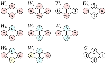
Figure 4. The $L$-invariant subspaces for the Laplacian matrix $L$ of the diamond graph $G$. A typical element of each invariant subspace is shown on the left, with the exception of $W_{0}=\{0\}\subseteq\mathbb{R}^{4}$, $W_{10}=\mathbb{R}^{4}$, and a reflection of $W_{5}$. The lattice of group orbits of $L$-invariant subspaces is shown on the right. The boxes indicate invariant subspaces that are not fixed point subspaces of the $\operatorname{Aut}(G)\times\mathbb{Z}_{2}$ action. The dashed arrows connect invariant subspaces with the same point stabilizer.

Assume that the state space of each cell has dimension $k=1$, and the internal dynamics is $f(s,x_{i})=sx_{i}+x_{i}^{3}$. We set $M=L$, and $H=[-1]\equiv-1$. Note that we identify the $1\times 1$ matrix $[-1]$ with a real number. Thus, System (3) becomes

(7) $$F_{i}(s,x)=sx_{i}+x_{i}^{3}-(Lx)_{i},\quad i\in\{1,2,3,4\}.$$

Thus we have a function $F:\mathbb{R}\times\mathbb{R}^{4}\to\mathbb{R}^{4}$ whose component functions are Equation (7). We search for solutions to $F(s,x)=0$, and we want to understand the bifurcations. As proved in [18], the $F$-invariant subspaces are the $L$-invariant subspaces. These are shown in Figure 4 .

The eigenvalues of $L$ are $\lambda=0$ with eigenvector $(1,1,1,1)$, $\lambda=2$ with eigenvector $(1,0,-1,0)$, and $\lambda=4$ with an eigenspace spanned by $(1,-1,1,-1)$ and $(0,1,0,-1)$.

The vector field $F$ is $\operatorname{Aut}(G)\times\mathbb{Z}_{2}$-equivariant, where $\operatorname{Aut}(G)=\langle(1\,3),(2\,4)\rangle\cong\mathbb{Z}_{2}\times\mathbb{Z}_{2}$ is the symmetry group of the graph $G$. The extra $\mathbb{Z}_{2}$ symmetry holds because $F(s,-x)=-F(s,x)$, that is, $F$ is odd. The vector field $F$ describes a coupled cell network which has more structure than symmetry alone. For example, the multiplicity 2 eigenvalue $\lambda=4$ is not caused by symmetry since all of the irreducible representations of $\mathbb{Z}_{2}\times\mathbb{Z}_{2}\times\mathbb{Z}_{2}$ are one-dimensional [11].

As described in Section 4, we have written a MATLAB^® program that computes the bifurcation diagrams of a large class of coupled cell networks systems. We solve Equation (7) on the diamond graph with the results shown in Figure 5. Our program computes one element in each group orbit of branches that is connected to the trivial branch, by recursively following daughter branches of BLIS bifurcations. The bifurcation points are indicated by the circles. If branches cross in this view but there is no circle, then the branches do not cross in $\mathbb{R}\times\mathbb{R}^{4}$ and there is not a bifurcation. We focus on the three highlighted bifurcation points of Figure 5 in the next three examples.

Figure 5. The complete bifurcation diagram of Equation (7). The invariant subspace of each branch is indicated. The invariant subspaces are described in Figure 4. This figure shows the bifurcation points that spawn BLIS branches that are neither BSE nor EBL branches, at $s=-2$ (Example 3.16), $s=2.5$ (Example 3.18), and $s=4$ (Example 3.17).

Example 3.16.

Figure 6. BLIS bifurcations $W_{1}\to W_{5}$ and $W_{1}\to W_{6}$ at $s=-2$, listed as Example 3.16(a) in Figure 1. There are also two pitchfork bifurcations shown that are BSE, EBL, and BLIS: $W_{6}\to W_{9}$ and $W_{5}\to W_{10}$, which are listed as Example 3.16(b) in Figure 1. Only one of the two branches is plotted in each case to avoid clutter. Note that this figure plots a different function of $x\in\mathbb{R}^{4}$ vs. $s$ than the one plotted in Figure 5. Plotting $x_{4}$ shows that only one of the $W_{6}$ branches has a bifurcation. See Example 3.16.

Continuing the example of the diamond graph, the solution branch in $W_{1}$ that bifurcates from the origin at $s=0$ undergoes two secondary bifurcations, at $s=-1$ and $s=-2$, as seen in Figure 5. In this example, we focus on the secondary bifurcation at $s=-2$, and the tertiary bifurcations of these daughters, as seen in the detailed bifurcation diagram in Figure 6. The bifurcation of the $W_{1}$ branch at $s=-2$ is a BLIS bifurcation that is neither an EBL nor a BSE bifurcation. This bifurcation is also described by [4, Theorem 8.2]. It is indicated in Figure 1 as 3.16(a). The daughters are two secondary branches in $W_{1}$ and $W_{5}$, and each of these branches undergoes a tertiary bifurcation which is a standard pitchfork bifurcation described by the BSE, EBL and BLIS. These pitchfork bifurcations are indicated in Figure 1 as 3.16(b).

Note that $W_{1}$ is not a fixed point subspace of the $\operatorname{Aut}(G)\times\mathbb{Z}_{2}$ action. The synchrony basis matrix for $W_{1}$ is $B_{1}:=[1\,1\,1\,1]^{T}$ with pseudoinverse $B_{1}^{+}=\frac{1}{4}[1\,1\,1\,1]$. Thus $B_{1}^{+}LB_{1}=0$ for the Laplacian matrix (6), and Theorem 3.12 says that $F(s,x)=0$ restricted to $W_{1}$ is

$$F_{B_{1}}(s,y)=sy+y^{3}=0.$$

This has three solutions, $y=0$ and $y=\pm\sqrt{-s}$. The solution $y=0$ is in $W_{0}$. The latter solutions are in $W_{1}$ but not in $W_{0}$. For $y=\sqrt{-s}$, the mother branch function $b_{m}:\mathbb{R}\to\mathbb{R}^{4}$ is $b_{m}(s)=\sqrt{-s}(1,1,1,1)$. We find that $D_{2}F_{B_{1}}(s,y)=s+3y^{2}$, and thus $D_{2}F_{B_{1}}(s,b_{m}(s))=-2s$. This eigenvalue of this matrix does not change sign, and Proposition 2.8 applies. The eigenvalues of $D_{2}F(s,b_{m}(s))$ are $-2s$, $1-s$, and $2-s$ (with multiplicity 2). We focus on the two BLIS bifurcations at $s=-2$ which have daughter branches in $W_{5}$ and $W_{6}$, respectively.

The synchrony basis matrix of $W_{5}$ is $B_{5}:=\left[\begin{smallmatrix}1&0&1&1\\ 0&1&0&0\end{smallmatrix}\right]^{T}$, and $B_{5}^{+}LB_{5}=\left[\begin{smallmatrix}1&-1\\ -3&3\end{smallmatrix}\right]$. Note that $B_{5}^{+}LB_{5}$ is the Laplacian matrix of the quotient digraph, which has an arrow with weight 1 from cell 2 to cell 1, and an arrow with weight 3 from cell 1 to cell 2. By Proposition 3.12, the system $F(s,x)=0$ restricted to $W_{5}$ is

(8) $$F_{B_{5}}(s,y)=(sy_{1}+y_{1}^{3}-(y_{1}-y_{2}),sy_{2}+y_{2}^{3}-3(y_{2}-y_{1}))=0.$$

The Jacobian matrix of $F_{B_{5}}$ is

$$D_{2}F_{B_{5}}(s,y)=\begin{bmatrix}s+3y_{1}^{2}-1&1\\ 3&s+3y_{2}^{2}-3\end{bmatrix},$$

and the Jacobian matrix evaluated at the mother branch is

$$J(s):=D_{2}F_{B_{5}}(s,b_{m}(s))=\begin{bmatrix}-2s-1&1\\ 3&-2s-3\end{bmatrix}.$$

The eigenvalues of $J(s)$ are $-2s$ and $-2(s+2)$. Thus there is a bifurcation at $s^{*}=2$ and the two components of Theorem 2.11 are

$$J(-2)=\begin{bmatrix}3&1\\ 3&1\end{bmatrix},\quad J^{\prime}(-2)=\begin{bmatrix}-2&0\\ 0&-2\end{bmatrix}.$$

We see that $N(J(-2))=\operatorname{Span}(\{(1,-3)\})$ is one-dimensional, and the $J^{\prime}(-2)(1,-3)=(-2,6)$ is not in $R(J(-2))=\operatorname{Span}(\{(1,1)\})$, so the hypotheses of Theorem 2.11 hold. There is exactly one daughter branch in $W_{5}$ bifurcating from the mother branch at $s=-2$.

Similarly, the synchrony basis matrix of $W_{6}$ is $B_{6}:=\left[\begin{smallmatrix}1&0&1&0\\ 0&1&0&1\end{smallmatrix}\right]^{T}$. The system $F(s,x)=0$ restricted to $W_{6}$ is

(9) $$F_{B_{6}}(s,y)=(sy_{1}+y_{1}^{3}-2(y_{1}-y_{2}),sy_{2}+y_{2}^{3}-2(y_{2}-y_{1}))=0.$$

The Jacobian matrix of $F_{B_{5}}$ is

$$D_{2}F_{B_{6}}(s,y)=\begin{bmatrix}s+3y_{1}^{2}-2&2\\ 2&s+3y_{2}^{2}-2\end{bmatrix},$$

and the Jacobian matrix evaluated at the mother branch is

$$J(s):=D_{2}F_{B_{6}}(s,b_{m}(s))=\begin{bmatrix}-2s-2&2\\ 2&-2s-2\end{bmatrix}.$$

The eigenvalues of $J(s)$ are $-2s$ and $-2(s+2)$. Thus there is a bifurcation at $s^{*}=2$ and the two components of Theorem 2.11 are

$$J(-2)=\begin{bmatrix}2&2\\ 2&2\end{bmatrix},\quad J^{\prime}(-2)=\begin{bmatrix}-2&0\\ 0&-2\end{bmatrix}.$$

We see that $N(J(-2))=\operatorname{Span}(\{(1,-1)\})$ is one-dimensional, and the $J^{\prime}(-2)(1,-1)=(-2,2)$ is not in $R(J(-2))=\operatorname{Span}(\{(1,1)\})$, so the hypotheses of Theorem 2.11 hold. There is exactly one daughter branch in $W_{6}$ bifurcating from the mother branch at $s=-2$.

Figure 6 shows these two bifurcations. Note that the restricted system (9) has a symmetry $(y_{1},y_{2})\mapsto(y_{2},y_{1})$ and consequently the bifurcation $W_{1}\to W_{6}$ is a pitchfork bifurcation within the restricted system (9). Within the full system in $\mathbb{R}\times\mathbb{R}^{4}$ there is no such symmetry, so our MATLAB^® code follows both branches. The lower $W_{6}$ branch in Figure 6 undergoes a bifurcation at $s\approx-2.4$, whereas the upper branch has no bifurcation. There is apparently no symmetry of the restricted system (8), and the bifurcation $W_{1}\to W_{6}$ is transcritical as expected.

Example 3.17.

The trivial branch in System (7) for the diamond graph has a double 0 eigenvalue at $s=4$. There is not a BSE at $(s,x)=(4,0)$ in Figure 5. The irreducible representations of $\operatorname{Aut}(G)\times\mathbb{Z}_{2}$ are all one-dimensional, so there is not an EBL bifurcation at that point. However, there are 3 BLIS branches that bifurcate from this point. The critical eigenspace of $D_{2}F(4,0)$ is the eigenspace of $L$ with eigenvalue $\lambda=4$, which is $E:=\operatorname{Span}(\{(1,-1,1,-1),(0,1,0,-1)\})$. We can use a shortcut to avoid calculations like those in Example 3.16, following Remark 2.12 (1) and (5). For each of the invariant subspaces $W_{i}$, there is a BLIS bifurcation from $W_{0}$ to $W_{i}$ if the intersection $E\cap W_{i}$ is one-dimensional. Consulting Figure 4, we see that $E\cap W_{2}=W_{2}$, $E\cap W_{3}=W_{3}$, and $E\cap W_{5}=\operatorname{Span}(\{(1,-3,1,1)\})$ are all one-dimensional, and $E\cap W_{1}=E\cap W_{4}=\{0\}$. It is the case that $E\cap W_{6}=W_{2}$ is one-dimensional, so the BLIS theorem says that there is a daughter branch in $W_{6}$, but this branch is also in $W_{2}$. Thus, we do not need to consider the invariant subspaces that contain $W_{2}$, $W_{3}$, and $W_{5}$ and we have found all the BLIS bifurcations: $W_{0}\to W_{2}$, $W_{0}\to W_{3}$, $W_{0}\to W_{5}$. These three bifurcating branches are seen in Figure 5.

Example 3.18.

The BLIS bifurcation of the mother branch $W_{5}$ to the daughter branch $W_{8}$ at $s=2.5$ is a BSE, but not an EBL bifurcation. For this bifurcation, we will not verify Condition (b) in Theorem 2.11 which is generically true, but focus on Condition (a). The system $F(s,x)=0$ restricted to $W_{5}$ was shown in Equation (8). We cannot easily solve that system to find the mother branch function $b_{m}(s)$ in closed form, but our MATLAB^® program finds numerical solutions. The program also gives a numerical approximation of the bifurcation point, and we can verify by hand that $F_{B_{5}}(\frac{5}{2},(\frac{1}{\sqrt{2}},-\sqrt{2}))=(0,0)$. Furthermore, $D_{2}F_{B_{5}}(\frac{5}{2},(\frac{1}{\sqrt{2}},-\sqrt{2}))$ is nonsingular, so the hypotheses of Proposition 2.8 hold. The system $F(s,x)=0$ restricted to $W_{8}$ is $F_{B_{8}}(s,y)=0$, where

$$F_{B_{8}}(s,y)=(sy_{1}+y_{1}^{3}-(2y_{1}-y_{2}-y_{3}),sy_{2}+y_{2}^{3}-(3y_{2}-2y_{1}-y_{3}),sy_{3}+y_{3}^{3}-(3y_{3}-2y_{1}-y_{2})).$$

The Jacobian matrix of $F_{B_{8}}$ is

$$D_{2}F_{B_{8}}(s,y)=\begin{bmatrix}s+3y_{1}^{2}-2&1&1\\ 2&s+3y_{2}^{2}-3&1\\ 2&1&s+3y_{3}^{2}-3\end{bmatrix}.$$

While we cannot find the mother branch function $b_{m}$, or $J(s)=D_{2}F_{B_{8}}(s,b_{m}(s))$, the Jacobian matrix evaluated at the bifurcation point is

$$\textstyle J(\frac{5}{2})=D_{2}F_{B_{8}}(\frac{5}{2},(\frac{1}{\sqrt{2}},-\sqrt{2},\frac{1}{\sqrt{2}})=\begin{bmatrix}2&1&1\\ 2&\frac{11}{2}&1\\ 2&1&1\end{bmatrix}.$$

This matrix has a simple zero eigenvalue with an eigenvector of $(1,0,-2)$. Thus, Condition (a) of Theorem 2.11 is satisfied. While we cannot prove that Condition (b) in the theorem holds, it is true generically, and our MATLAB^® program does not check it. The program follows the daughter branches in $W_{8}$, suggesting that Condition (b) is true. This BLIS bifurcation is also a BSE, since the $4\times 4$ Jacobian matrix evaluated at the bifurcation point has a simple 0 eigenvalue. There is no symmetry, so this is not an EBL bifurcation.

3.3. PDE Examples

Consider the PDE

(10) $$\Delta u+su+N(u)=0$$

for $u:\Omega\to\mathbb{R}$ with $0\,$-Dirichlet boundary conditions, where $\Omega$ is a region in $\mathbb{R}^{n}$, and $N:\mathbb{R}\to\mathbb{R}$ is a nonlinearity which satisfies $N(0)=N^{\prime}(0)=0$. We seek zeros of the function $F:\mathbb{R}\times H\to H$ defined by

$$F(s,u)=u+\Delta^{-1}(su+N(u)),$$

where $H$ is the Sobolev space $H_{0}^{1,2}(\Omega)$. We usually choose the subcritical, superlinear nonlinearity $N(u)=u^{3}$, as in [12, 16]. In this case and others, regularity theory [6] gives that a zero of $F$ is twice differentiable and hence a classical solution to the PDE.

The eigenvalue equation associated with PDE (10) is $\Delta u+\lambda u=0$, on the same region with $0\,$-Dirichlet boundary conditions. It is well-known [5] that the eigenvalues are real and satisfy $0<\lambda_{1}<\lambda_{2}\leq\lambda_{3}\cdots\to\infty$ . All BSE, EBL, and BLIS bifurcations from the trivial solution are described by Theorem 2.11 with $W_{m}=\{0\}$. For the current function $F$, the operator $J(s)=D_{2}F(s,0)$ defined in Theorem 2.11 has eigenvalues $\{1-s/\lambda_{i}\mid i\in\mathbb{N}\}$. We expect that the branch of trivial solutions has a bifurcation of some sort at $(s,u)=(\lambda_{i},0)$. Suppose we find an invariant subspace $W_{d}\subseteq H$ such that $N(J(\lambda_{i}))=\operatorname{Span}(\{x_{0}\})$, in the notation of Theorem 2.11. We see that all of the conditions of the Theorem hold. The second part of Condition (a) holds because $H$ is a Hilbert space and $\Delta^{-1}$ is self-adjoint. Thus, the range of $J(\lambda_{i})$ is the orthogonal complement of the null space, which has codimension one. Condition (b) holds because $J^{\prime}(s)=\Delta^{-1}$, and therefore $J^{\prime}(\lambda_{i})(x_{0})=x_{0}/\lambda_{i}\not\in R(J(\lambda_{i}))$.

Example 3.19.

Consider PDE (10). Since $\lambda_{1}$ is simple, the BSE and the BLIS apply at the point $(s,u)=(\lambda_{1},0)$. There is a unique branch of nontrivial solutions that bifurcates from this point. An explicit example is the PDE

$$\Delta u+su+u^{2}=0,$$

for which there is a transcritical bifurcation, and for which the EBL does not apply. Note the similarity to Example 3.2.

Example 3.20.

Consider PDE (10) with $N$ odd. Then $F(s,-u)=-F(s,u)$, and the bifurcation at $(s,u)=(\lambda_{1},0)$ is a pitchfork bifurcation. In this case, the BSE, EBL, and BLIS all apply. An explicit example is the PDE

$$\Delta u+su+u^{3}=0.$$

Note the similarity to Example 3.1.

Example 3.21.

Consider PDE (10) with the square domain, $\Omega=(0,1)^{2}$. The eigenvalues and eigenfunctions of the Laplacian can be explicitly computed as

$$\psi_{n,m}(x,y)=\sin(n\pi x)\sin(m\pi y),\quad\lambda_{n,m}=(n^{2}+m^{2})\pi^{2},$$

with $n,m\in\mathbb{N}$. Note that $0<\lambda_{1,1}<\lambda_{1,2}=\lambda_{2,1}$. The EBL applies to the bifurcation at $(s,u)=(\lambda_{1,2},0)$, but BSE does not apply. The group $\operatorname{Aut}(\Omega)$ is the symmetry of the square, and that group acts on $H$. The fixed point subspaces $\{u\in H:u(x,y)=u(y,x)\}$ and $\{u\in H:u(x,y)=u(1-x,y)\}$ are $F$-invariant and the BLIS applies.

Figure 7. The critical eigenspace $V$ at the bifurcation point $(s^{*},0)$ in Example 3.22, where $s^{*}=10\pi^{2}$. The diagonal lines are intersections of two fixed point subspaces with $V$ and lead to EBL bifurcations. The horizontal dashed line is the intersection of $W_{d}$ with $V$ and leads to a BLIS bifurcation. The vertical dashed line leads to another similar BLIS bifurcation. The three line types correspond to the three group orbits of bifurcating solutions.

Example 3.22.

Consider bifurcation point $(s,u)=(\lambda_{1,3},0)$ for PDE (10) with the square domain, $\Omega=(0,1)^{2}$, with eigenvalues and eigenfunction listed in Example 3.21. The eigenvalue $\lambda_{1,3}=\lambda_{3,1}$ is not simple so BSE does not apply. The EBL predicts two group orbits of daughter branches, and the BLIS predicts these two as well as a third group orbit of bifurcating solutions. These are shown in Figure 1 as 3.22(a) and (b), respectively.

The bifurcation of the trivial solution at $s=\lambda_{1,3}$ has a 2-dimensional critical eigenspace

$$V=N(D_{2}F(\lambda_{1,3},0))=\operatorname{Span}(\{\psi_{1,3},\psi_{3,1}\}).$$

Figure 7 shows the eigenfunctions in $V$ that give rise to 8 solution branches, in three group orbits, that bifurcate from the trivial solution at $s=\lambda_{3,1}=10\pi^{2}$. We count this as 8 solution branches following Remark 2.12(7).

The function $F$ is $\mathbb{D}_{4}\times\mathbb{Z}_{2}$-equivariant, where the symmetry group $\mathbb{D}_{4}$ of the square acts on $H$ in the natural way and $\mathbb{Z}_{2}$ acts as $u\mapsto-u$. The $\mathbb{D}_{4}\times\mathbb{Z}_{2}$ action on $V$, modulo the kernel of the action, is isomorphic to $\mathbb{D}_{2}$, and is generated by $(\psi_{1,3},\psi_{3,1})\mapsto(\psi_{3,1},\psi_{1,3})$ and $(\psi_{1,3},\psi_{3,1})\mapsto-(\psi_{1,3},\psi_{3,1})$. The EBL says that $\operatorname{Span}(\{\psi_{1,3}+\psi_{3,1}\})$ and $\operatorname{Span}(\{\psi_{1,3}-\psi_{3,1}\})$, the diagonals in Figure 7, give rise to branches in two fixed-point subspaces in $H$. The bifurcating solutions are either even or odd in each of the reflection lines of the square.

The BLIS shows that there is a bifurcating branch in $\mathbb{R}\times W_{d}$, where

$$W_{d}:=\{u\in H\mid\ u(x,1-y)=u(x,y)\text{ for }(x,y)\in(0,1)\times(0,1)\text{ and }$$

$$u(x,\textstyle\frac{2}{3}-y)=-u(x,y)\text{ for }(x,y)\in(0,1)\times(0,\textstyle\frac{2}{3})\}.$$

The intersection of $W_{d}$ with $V$ is $\operatorname{Span}(\{\psi_{1,3}\})$, depicted by the horizontal dashed line in Figure 7. The stability of the trivial branch is determined by $J(s)=D_{2}F_{d}(s,0)$, which has a simple eigenvalue equal to $1-s/\lambda_{1,3}$ with the critical eigenvector $\psi_{1,3}$. The symmetry of the square implies that there is another invariant subspace that intersects $V$ in $\operatorname{Span}(\{\psi_{3,1}\})$, leading to another BLIS bifurcation. See [16] for numerical results of these bifurcating branches, as well as other nearby primary and secondary solution branches.

Example 3.23.

In [12] we investigate the PDE $\Delta u+su+u^{3}=0$ on the cube $(0,\pi)^{3}$ with $0\,$-Dirichlet boundary conditions. Here the eigenvalues of the Laplacian are $\lambda_{\ell,m,n}=\ell^{2}+m^{2}+n^{2}$, with eigenfunctions $\psi_{\ell,m,n}(x,y,z)=\sin(\ell x)\sin(my)\sin(nz)$. There are 99 group orbits of fixed point subspaces of the symmetry group of the cube acting on the function space $H$. These are called symmetry types, denoted $S_{0}$ through $S_{98}$. The paper features the bifurcation of the trivial branch at $s^{*}=\lambda_{1,2,3}=14$, for which $J(s^{*})$ has a 6-dimensional critical eigenspace.

1. This bifurcation has 4 group orbits of EBL branches, indicated in [12, Figures 23 and 25]. These have symmetry types $S_{11}$, $S_{12}$, $S_{22}$, and $S_{23}$.

2. There are also 2 additional BLIS branches that are not EBL branches. The invariant subspaces are spaces of functions with odd reflection symmetry at $z=\pi/3$ and $z=2\pi/3$. These are shown in [12, Figure 25] with symmetry type $S_{52}$, with critical eigenfunction $\psi_{1,2,3}$, and the third solution with symmetry type $S_{44}$, with critical eigenfunction $\psi_{1,2,3}+\psi_{2,1,3}$. Thus there are 6 group orbits of BLIS branches that bifurcate from $(s,u)=(14,0)$.

3. In addition, there are 13 group orbits of solution branches that are not BLIS branches.

The branches in Parts (a) and (b) are simple to follow, since the critical eigenvector is determined by Theorem 2.11. Following BLIS branches is like shooting fish in a barrel. In contrast, the 13 group orbits of non BLIS branches are found by a random search of the 6-dimensional critical eigenspace. Many hours of computing time were required to find them, and it is possible that some eluded detection. We are reasonably confident we have found all of the branches, with the help of index theory as described in [12].

4. Numerical Implementation

We wrote a MATLAB^® program, available at the GitHub repository [15]. It approximates solutions to the system of $n$ equations

(11) $$F(s,x)_{i}:=f(s,x_{i})-(Mx)_{i}=0,\quad i\in\{1,2,\ldots,n\}$$

for the components of $x\in\mathbb{R}^{n}$. These are equilibrium solutions of Equation (4), with $k=1$ (so $x_{i}\in\mathbb{R}$) and the $1\times 1$ coupling matrix $H=-1$. The input data for the program includes the weighted adjacency matrix $M\in\mathbb{R}^{n\times n}$, the nonlinearity $f:\mathbb{R}^{2}\rightarrow\mathbb{R}$, the permutations that commute with $M$, the $M$-invariant polydiagonal subspaces, and the containment lattice of the $M$-invariant subspaces.

Figures 5 and 6 show bifurcation diagrams with $M$ chosen to be the Laplacian matrix in Equation (6). We made text files which input the information shown in Figure 4. We chose

(12) $$f(s,x)=sx+x^{3},$$

to yield Equation (7). Other choices of $f$, predefined in our MATLAB^® code, are

$$f(s,x)=sx+\alpha x^{2}-x^{3}\text{ and }f(s,x)=sx+x^{3}-\beta x^{5},$$

where $\alpha$ and $\beta$ are parameters which cannot be scaled away. We do not require that $f$ is odd in the second variable, but the program treats $f$ odd and $f$ not odd differently. The $M$-invariant synchrony subspaces are $F$-invariant for all $f$. The $M$-invariant anti-synchrony subspaces are $F$-invariant if $f$ is odd (see [18]).

We frequently assume $f$ satisfies $f(s,0)=0$, $D_{1}f(s,x)=x$, and $D_{2}f(s,0)=s$ for all $s$, as in the above examples. This has the advantage that the stability of the trivial branch is easy to compute. For the trivial branch, with $b_{m}(s)=0$ and $W_{d}=\mathbb{R}^{n}$, the stability matrix $J(s)=sI_{n}-M$ is easily analyzed based on the eigenvalues of $M$ (see Equation (2)). Our program works for any smooth $f$, although if $f(s,0)\neq 0$, then an approximate solution must be supplied to the program as a starting point for the first branch. For example we have tested

$$f(s,x)=(s^{2}-1)x\pm x^{3},\quad f(s,x)=sx+x^{3}+1.$$

We now describe the general algorithms that, when implemented, can generate numerical bifurcation results for networks such as those displayed in Figures 5 and 6. There are four essential processes involved:

1. Compute the lattice of invariant subspaces.

2. Follow branches, given a starting point, the invariant subspace, and initial direction.

3. Detect bifurcation points, which are the starting points of daughter branches.

4. Use BLIS to find the invariant subspace and initial direction of each daughter branch.

For the first process, we start with the matrix $M$ in (11) (typically the graph Laplacian). The algorithm described in [18] and implemented on that article’s GitHub repository [17] finds all of the $M$-invariant polydiagonal subspaces and the lattice showing which subspaces are contained in which others. For example, the information in Figure 4 can be computed with this program.

The weighted analytic matrix $M$, invariant subspaces, lattice of inclusion, and $\operatorname{Aut}(G)$ information is passed to the MATLAB^® program by four text files, as described in the user’s manual available at [15].

Given these four text files as inputs, the MATLAB^® code posted on the current paper’s GitHub repository [15] computes the bifurcation diagrams showing all of the solutions to Equation (11) that are within the strip $s_{\text{min}}\leq s\leq s_{\text{max}}$ and connected by a series of BLIS bifurcations to the starting solution, usually $x=0$, $s=s_{\text{min}}$. The input parameters are changed by editing the MATLAB^® code.

Branch following is achieved by employing a new version of the so-called tGNGA (tangent gradient Newton Galerkin Algorithm) described in [12]. The added feature is that the computations are done within the invariant subspace. That is, we solve Equation (5) (with $H=-1$) rather than Equation (11). This speeds up the computations greatly, especially in examples where $n$ is large and $d$ is small.

The input to the tGNGA is the invariant subspace $W_{m}$ of the branch, a single point $(\tilde{s},\tilde{x})\in\mathbb{R}\times W_{m}$, and a tangent vector to the branch in $(\tilde{s},\tilde{x})\in\mathbb{R}\times W_{m}$. Typically, the first branch has $\tilde{x}=0$ and $W_{m}=\{0\}$. After that, the initial point is a bifurcation point on a previously computed branch.

The branch following algorithm needs to stop the branch at a bifurcation point when it is the daughter branch. If the branch continues past the bifurcation point, then it can potentially continue past another bifurcation point and cause an infinite loop in the MATLAB^® program.

Detecting bifurcation points on a mother branch in $\mathbb{R}\times W_{m}$ is done using the BLIS. The Morse Index, which is a non-negative integer, is an important feature in our GNGA [11, 12, 16]. It is replaced by a vector of non-negative integers in our new code. Let $\mathcal{D}$ be the set of $F$-invariant subspaces of System (11) that contain $W_{m}$. As described in [18], $\mathcal{D}$ is different depending on whether or not $f$ is odd. These are the possible daughter subspaces. At each computed point on the mother branch, the eigenvalues of the Jacobian, restricted to each $W\in\mathcal{D}$, are computed, and a list of the number of eigenvalues with negative real part is recorded. This is the signature list. Recall that the matrix $M$ in Equation (11) need not be symmetric, so the eigenvalues of the Jacobian are not necessarily real. If any of the numbers on the signature list changes between two points, the secant method is used to find the point where an eigenvalue has zero real part. At a fold point, the signature of the Jacobian, restricted to $W_{m}$, changes by 1 and this is not a bifurcation point. If any other number on the signature list changes by 1, the point where the corresponding eigenvalue is 0 is a BLIS bifurcation point, and the corresponding critical eigenvector is computed.

The invariant subspace of the daughter branch is the smallest $W\in\mathcal{D}$ that contains the critical eigenvector. Care must be taken to follow only one daughter branch if several of them are related by the $\operatorname{Aut}(G)\times\mathbb{Z}_{2}$ symmetry. Then the bifurcation point, the invariant subspace, and the critical eigenvector are put into a queue to start the daughter branch with the tGNGA. We do not check Condition (b) in Theorem 2.11. This condition is generically true, and it is observed to be true in all of the bifurcations we have computed. In this way, we follow one branch in each group orbit of branches that are connected to the first branch (usually the trivial branch) by a sequence of BLIS bifurcations.

5. Conclusion

We have presented the Bifurcation Lemma for Invariant Subspaces (BLIS), which describes most generic bifurcations of solutions to $F(s,x)=0$, for $F:\mathbb{R}\times X\to X$. The space $X$ can be the Euclidean space $\mathbb{R}^{n}$, or more generally a Banach space. Thus, the theory applies to PDE. The theory of Bifurcation from Simple Eigenvalues (BSE) describes the simplest case. The BLIS is BSE applied to nested invariant subspaces of $F$. The BLIS allows the analysis of some bifurcations with multiple 0 eigenvalues. The Equivariant Branching Lemma (EBL) has been a powerful tool for describing bifurcations where high multiplicity of a zero eigenvalue is caused by the symmetry of the system. The EBL is a special case of the BLIS. Many coupled cell networks have invariant subspaces beyond those caused by symmetry, and the BLIS can describe bifurcations in such systems. We have written a freely available MATLAB^® program that computes the solution branches in a class of coupled cell networks.

While the BLIS does not describe all steady state bifurcations, in many examples most or all of the bifurcating branches are predicted by this simple theorem which is easy to apply.

References

- [1] Manuela A. D. Aguiar and Ana Paula S. Dias. The lattice of synchrony subspaces of a coupled cell network: characterization and computation algorithm. J. Nonlinear Sci., 24(6):949–996, 2014.
- [2] G. Cicogna. Symmetry breakdown from bifurcation. Lett. Nuovo Cimento (2), 31(17):600–602, 1981.
- [3] Michael G. Crandall and Paul H. Rabinowitz. Bifurcation from simple eigenvalues. J. Functional Analysis, 8:321–340, 1971.
- [4] Alessio Franci, Martin Golubitsky, Ian Stewart, Anastasia Bizyaeva, and Naomi E. Leonard. Breaking indecision in multiagent, multioption dynamics. SIAM Journal on Applied Dynamical Systems, 22(3):1780–1817, 2023.
- [5] D. Gilbarg and N.S. Trudinger. Elliptic Partial Differential Equations of Second Order. Classics in Mathematics. Springer Berlin Heidelberg, 2001.
- [6] David Gilbarg and Neil S. Trudinger. Generalized Solutions and Regularity, pages 177–218. Springer Berlin Heidelberg, Berlin, Heidelberg, 2001.
- [7] Martin Golubitsky and David G. Schaeffer. Singularities and groups in bifurcation theory. Volume I, volume 51 of Appl. Math. Sci. Springer, Cham, 1985.
- [8] Martin Golubitsky and Ian Stewart. Dynamics and Bifurcation in Networks: Theory and Applications of Coupled Differential Equations. Society for Industrial and Applied Mathematics, Philadelphia, PA, 2023.
- [9] Martin Golubitsky, Ian Stewart, and David G. Schaeffer. Singularities and groups in bifurcation theory. Vol. II, volume 69 of Applied Mathematical Sciences. Springer-Verlag, New York, 1988.
- [10] Hiroko Kamei and Peter J. A. Cock. Computation of balanced equivalence relations and their lattice for a coupled cell network. SIAM J. Appl. Dyn. Syst., 12(1):352–382, 2013.
- [11] John M. Neuberger, Nándor Sieben, and James W. Swift. Automated bifurcation analysis for nonlinear elliptic partial difference equations on graphs. Internat. J. Bifur. Chaos Appl. Sci. Engrg., 19(8):2531–2556, 2009.
- [12] John M. Neuberger, Nándor Sieben, and James W. Swift. Newton’s method and symmetry for semilinear elliptic PDE on the cube. SIAM J. Appl. Dyn. Syst., 12(3):1237–1279, 2013.
- [13] John M. Neuberger, Nándor Sieben, and James W. Swift. Invariant Synchrony Subspaces of Sets of Matrices (companion web site), 2019. https://jan.ucc.nau.edu/ns46/invariant.
- [14] John M. Neuberger, Nándor Sieben, and James W. Swift. Invariant synchrony subspaces of sets of matrices. SIAM J. Appl. Dyn. Syst., 19(2):964–993, 2020.
- [15] John M. Neuberger, Nándor Sieben, and James W. Swift. Github repository, https://github.com/jwswift/BLIS/, 2023.
- [16] John M. Neuberger and James W. Swift. Newton’s method and Morse index for semilinear elliptic PDEs. Internat. J. Bifur. Chaos Appl. Sci. Engrg., 11(3):801–820, 2001.
- [17] Eddie Nijholt, Nándor Sieben, and James W. Swift. Github repository, https://github.com/jwswift/Anti-Synchrony-Subspaces/, 2022.
- [18] Eddie Nijholt, Nándor Sieben, and James W. Swift. Invariant synchrony and anti-synchrony subspaces of weighted networks. J. Nonlinear Sci., 33(4):38, 2023. Id/No 63.
- [19] A. Vanderbauwhede. Local bifurcation and symmetry, volume 75 of Research Notes in Mathematics. Pitman (Advanced Publishing Program), Boston, MA, 1982.