In this paper, we describe an algorithm for approximating functions of the form $f(x)={\langle\sigma(\mu),x^{\mu}\rangle}$ over $[0,1]\subset\mathbb{R}$, where $\sigma(\mu)$ is some distribution supported on $[a,b]$, with $0<a<b<\infty$. One example from this class of functions is $x^{c}(\log{x})^{m}=(-1)^{m}{\langle\delta^{(m)}(\mu-c),x^{\mu}\rangle}$, where $a\leq c\leq b$ and $m\geq 0$ is an integer. Given the desired accuracy $\epsilon$ and the values of $a$ and $b$, our method determines a priori a collection of non-integer powers $t_{1}$, $t_{2}$, …, $t_{N}$, so that the functions are approximated by series of the form $f(x)\approx\sum_{j=1}^{N}c_{j}x^{t_{j}}$, and a set of collocation points $x_{1}$, $x_{2}$, …, $x_{N}$, such that the expansion coefficients can be found by collocating the function at these points. We prove that our method has a small uniform approximation error which is proportional to $\epsilon$ multiplied by some small constants. We demonstrate the performance of our algorithm with several numerical experiments, and show that the number of singular powers and collocation points grows as $N=O(\log{\frac{1}{\epsilon}})$.

On the Approximation of Singular Functions by Series of Non-integer Powers

Mohan Zhao$\mbox{}^{\dagger\,\diamond}$ and Kirill Serkh$\mbox{}^{\ddagger\,\diamond}$

University of Toronto NA Technical Report

v2,

$\mbox{}^{\diamond}$This author’s work was supported in part by the NSERC Discovery Grants RGPIN-2020-06022 and DGECR-2020-00356.

$\mbox{}^{\dagger}$ Dept. of Computer Science, University of Toronto, Toronto, ON M5S 2E4

Corresponding author. Email: mohan.zhao@mail.utoronto.ca

$\mbox{}^{\ddagger}$ Dept. of Math. and Computer Science, University of Toronto, Toronto, ON M5S 2E4

Email: kserkh@math.toronto.edu

Keywords: approximation theory, singular functions, singular value decompositions, corners, endpoint singularities, Laplace transforms, partial differential equations

1 Introduction

The approximation of functions with singularities is a central topic in approximation theory. One motivating application is the efficient representation of solutions to partial differential equations (PDEs) on nonsmooth geometries or with discontinuous data, which are known to be characterized by branch-point singularities. Substantial progress has been made in this area, with perhaps the most common approach being rational approximation (as well as variations of rational approximation). Alternative approaches include approximation schemes for smooth functions on the real line, applied after a change of variables to ensure a rapid function decay and the translation of singularities to infinity, and schemes that make use of basis functions obtained through the discretization of certain integral operators. If the dominant characteristics of the functions to be approximated are known a priori, a class of methods called expert-driven approximation can also be used.

Rational approximation is a classical and well-established method for approximating functions with singularities, using rational basis functions determined by their poles and residues, in the form $\sum_{j=1}^{m}\frac{a_{j}}{z-z_{j}}$, or by their weights in barycentric representations $\sum_{j=1}^{m}\frac{w_{j}f_{j}}{z-z_{j}}/\sum_{j=1}^{m}\frac{w_{j}}{z-z_{j}}$. In 1964, Newman proved that there exists an $n$-th order rational approximation to the function $f(x)=|x|$ on $[-1,1]$, converging at a rate of $O(\exp(-C\sqrt{n}))$ [24] (the polynomial approximation to $|x|$ on $[-1,1]$ can only achieve a convergence rate no better than $O(n^{-1})$). Furthermore, he observed that the same approximation also applies to the functions $f(x)=\sqrt{x}$ and $f(x)=x^{\alpha}$ on $[0,1]$, where $\alpha>0$. Notably, Newman’s approximation utilizes poles that are clustered exponentially and symmetrically around zero along the imaginary axis.

Numerous papers have been published on rational approximation methods for functions with singularities since Newman’s discovery (see, for example, [10], [30], [21], [7]). The best possible rational approximation is the so-called minimax approximation, which minimizes the maximum uniform approximation error between the function and its rational approximation. However, this minimax approximation is not easy to find and is not necessarily unique in the complex plane [13]. In practice, it turns out that the poles of the rational approximation can often be determined a priori, similar to those employed in Newman’s method, to achieve a root-exponential convergence rate. One such method is Stenger’s approximation [31], which involves interpolating the functions at a set of preassigned points exponentially clustered near the endpoints of the interval, in a rational basis with poles that are exponentially clustered at the endpoints.

While Stenger’s method uses explicit formulas for the rational approximations, the residues can also be found numerically. In fact, if the poles are determined a priori, one can oversample the function and use the least-squares method to determine the residues which minimize the maximum approximation error. A class of methods utilizing this technique is known as lightning methods, which have been designed to approximate solutions of Laplace ([12], [11]) and Helmholtz ([11]) equations on two-dimensional domains with corners. Lightning methods employ rational functions with preassigned poles that cluster exponentially around the corner singularities along rays terminating at the singularities. It was proved in [12] that any set of $n$ complex poles exhibiting exponential clustering, with spacing scaling as $O(n^{-1/2})$, can achieve root-exponential rates of convergence $O(\exp(-C\sqrt{n}))$. On more general geometries, the adaptive Antoulas-Anderson (AAA) algorithm [23] is an efficient and flexible nonlinear method that was developed to be domain-independent. The AAA method employs rational barycentric representations in the real or complex plane, incrementally increases the approximation order during iterations, and dynamically selects poles using a greedy algorithm. To determine the weights in the rational barycentric representations, the algorithm likewise solves a least-squares problem at each iteration.

While all of the aforementioned methods can achieve root-exponential rates of convergence, Trefethen et al. ([34]) made a key observation that the constant $C$ in the rates of convergence $O(\exp(-C\sqrt{n}))$ can be improved for most rational approximation methods by employing poles with tapered exponential clustering around singularities, such that the clustering density on a logarithmic scale tapers off linearly to zero near the singularities.

Rational approximation can also be applied after a change of variables. An approach referred to as reciprocal-log approximation [22] uses approximations of the form $r(\log{z})$, where $r(s)$ is an $n$-th degree rational function with poles determined a priori, either lying on a parabolic contour or confluent at the same point in the complex plane. Similarly to lightning methods, the coefficients are determined through a linear least-squares problem using collocation points that cluster exponentially around $z=0$. This method converges at a rate of $O(\exp(-Cn))$ or $O(\exp(-Cn/\log{n}))$ for functions with branch-point singularities, depending on the form of the approximation and the function’s behaviour in the complex plane.

An alternative approach is to use a combination of a change of variables and an approximation scheme that converges rapidly for smooth functions on the real line. By applying smooth transformations to functions with singularities at the endpoints of some finite intervals on the real line, they can be transformed into rapidly decaying functions, with the singularities mapped to the point at infinity. After this transformation, such functions can be approximated accurately using the Sinc approximation, by an $n$-term truncated Sinc expansion. Two primary approaches of this type have been developed: the SE-Sinc and DE-Sinc approximations (see, for example, [32], [25] and [20]). The SE-Sinc approximation combines the single-exponential transformation with the Sinc approximation, resulting in a convergence rate of $O(\exp(-C\sqrt{n}))$, while the DE-Sinc approximation combines the double-exponential transformation with the Sinc approximation, to further improve the convergence rate to $O(\exp(-Cn/\log{n}))$.

While the aforementioned methods require no special knowledge of the singularities being approximated, a class of methods known as expert-driven approximation can be used to leverage such information. For example, one can leverage knowledge of the leading terms in the asymptotic expansion of the singularity to achieve a smaller approximation error. This information is often available in the solutions of boundary value problems for PDEs on domain with corners—as revealed by Lehman ([18]) and Wasow ([35]), the solutions of the Dirichlet problem for linear second order elliptic PDEs have singular expansions in terms of the form $r^{\alpha}(r^{q}\log{r})^{m}\varphi(\theta)$, $\varphi$ is a smooth function, $r$ is the radial distance from the singularity, $\alpha\in\mathbb{R}$, $\alpha\geq\frac{1}{2}$, $q,m\in\mathbb{Z}$, $q\geq 1$ and $m\geq 0$. Many well-developed methods fall under the category of expert-driven approximation, such as the method of auxiliary mapping (see, for example, [19], [1]), in which an analytic change of variables is used to lessen the singular behaviour of the function, and enriched approximation methods (see, for example, [15]), in which singular basis functions are used to augment a conventional basis. Some examples of enriched approximation methods include extended/generalized finite element methods (see, for example, [26], [8], [9]), enriched spectral and pseudo-spectral methods (see, for example, [5], [12], [27]), and integral equation methods using singular basis functions (see, for example, [28] and [29]).

Based on the idea that the functions we are interested in approximating often belong to the range of certain integral operators, a much different class of approaches can also be used. One such method was proposed by Beylkin and Monzón [4], and involves representing a function by a linear combination of exponential terms with complex-valued exponents and coefficients. This method is motivated by the observation that many functions admit representations by exponential integrals over contours in the complex plane, which can then be discretized by quadrature. Instead of starting with a contour integral, the existence of such representations is only assumed implicitly, and the exponents (which they also call nodes) are obtained by finding the roots of a c-eigenpolynomial corresponding to a Hankel matrix, constructed from uniform samples of the function over the interval, while the coefficients (or weights) are determined via a Vandermonde system. This method can be highly effective for representing functions, though we note that their primary focus is on minimizing the error at the sample points, and for singular functions, they only emphasize the error on a subinterval which excludes the singularities.

In this paper, we present a method for approximating functions with an endpoint singularity over $[0,1]\subset\mathbb{R}$ or, more generally, a curve $\Gamma\subset\mathbb{C}$, where the functions have the form $f(x)=\int_{a}^{b}x^{\mu}\sigma(\mu)\,d\mu$, where $0<a<b<\infty$, $x\in[0,1]$ or $x\in\Gamma$, and $\sigma(\mu)$ is some signed Radon measure over $[a,b]$ or some distribution supported on $[a,b]$. Some examples of such functions are $x^{c}=\int_{a}^{b}x^{\mu}\delta(\mu-c)\,d\mu$ and $x^{c}(\log{x})^{m}=(-1)^{m}\int_{a}^{b}x^{\mu}\delta^{(m)}(\mu-c)\,d\mu$, where $a\leq c\leq b$, $m\in\mathbb{Z}$ and $m\geq 0$. Our method represents these functions as expansions of the form $\widehat{f}_{N}(x)=\sum_{j=1}^{N}\widehat{c}_{j}x^{t_{j}}$, so that ${\lVert f-\widehat{f}_{N}\rVert}_{L^{\infty}[0,1]}\approx\epsilon$, where the singular powers $t_{1}$, $t_{2}$, …, $t_{N}$ are determined a priori based on the desired approximation accuracy $\epsilon$ and the values of $a$ and $b$. The coefficients of the expansion are determined by numerically solving a Vandermonde-like collocation problem

$$\begin{pmatrix}x^{t_{1}}_{1}&x^{t_{2}}_{1}&\ \ldots&\ x^{t_{N}}_{1}\\ x^{t_{1}}_{2}&x^{t_{2}}_{2}&\ \ldots&\ x^{t_{N}}_{2}\\ \vdots&\vdots&\ \ddots&\vdots\\ x^{t_{1}}_{N}&x^{t_{2}}_{N}&\ \ldots&\ x^{t_{N}}_{N}\end{pmatrix}\begin{pmatrix}c_{1}\\ c_{2}\\ \vdots\\ c_{N}\end{pmatrix}=\begin{pmatrix}f(x_{1})\\ f(x_{2})\\ \vdots\\ f(x_{N})\end{pmatrix}$$ (1)

for $f(x)$ at the points $x_{1}$, $x_{2}$, …, $x_{N}$, where the collocation points are likewise determined a priori by $\epsilon$, $a$ and $b$. We show that these collocation points cluster tapered-exponentially near the singularities at $x=0$. We also show numerically that, in order to obtain a uniform approximation error of $\epsilon$, the number of basis functions and collocation points grows as $N=O(\log{\frac{1}{\epsilon}})$.

Notice that our method focuses on functions $f(x)$ that are in the range of the truncated Laplace transform after the change of variable $x=e^{-s}$, with $f(e^{-s})=\int_{a}^{b}e^{-s\mu}\sigma{(\mu)}\,d\mu$. The reciprocal-log approximation shares a similar idea. It specializes in approximating functions with branch-point singularities, such as $x^{\mu}$ on $[0,1]$, which are transformed into decaying exponential terms $e^{-s\mu}$ when the same change of variable is applied. Their approach leverages the fact that certain rational approximations can be obtained to approximate these exponential terms with an exponential rate of convergence. Consequently, $x^{\mu}$ can be approximated with an exponential rate of convergence using a rational approximation $r(s)$ with the change of variable $s=-\log{x}$. In contrast, our method relies on the discretization of the integral representation of $f(e^{-s})$ through the use of the singular value decomposition of the truncated Laplace transform. This procedure yields the quadrature nodes that enable us to approximate $f(x)$ using singular powers. The methodology in [4] also bears certain similarities with our method, in that they assume implicit integral representations of the functions, with decaying exponential kernels. However, rather than directly discretizing the integrals, they identify the exponential terms and coefficients for approximation through an analysis of the singular value decomposition of some Hankel matrix constructed from the function values.

In contrast to rational approximation which converges only at a root-exponential rate, our method converges exponentially. When compared to the DE-Sinc approximation method which requires a large number of collocation points placed at the both endpoints after applying the smooth transformation (even when singularities only happen at only one endpoint), and reciprocal-log approximation which uses many collocation points together with least squares, our method has a small number both of basis functions and collocation points, such that the coefficients can be determined via a square, low-dimensional Vandermonde-like system. Unlike the method proposed by Beylkin and Monzón [4], which only ensures an accurate approximation at equidistant points, our method ensures a small uniform error over the entire interval. Compared to expert-driven approximation, our method does not require any prior knowledge of the singularity types, besides the values of $a$ and $b$, and the resulting basis functions depend only on these values, together with the precision $\epsilon$.

The structure of this paper is as follows. Section 2 reviews the truncated Laplace transform and the truncated singular value decomposition. Section 3 demonstrates some numerical findings about the singular value decomposition of the truncated Laplace transform. Section 4 develops the main analytical tools of this paper. Section 5 describes some numerical experiments which provide conditions for the practical use of the theorems in Section 4. Section 6 shows that functions of the form $f(x)=\int_{a}^{b}x^{\mu}\sigma(\mu)\,d\mu$ can be approximated uniformly by expansions in singular powers. Section 7 shows that the coefficients of such expansions can be obtained numerically by solving a Vandermonde-like system, and provides a bound for the uniform approximation error. Section 8 illustrates that the previous results can be extended to the case where the measure is replaced by a distribution. Section 9 shows that, in practice, the algorithm can be applied using a smaller number of basis functions and collocation points than stated in Section 7. Finally, Section 10 presents several numerical experiments to demonstrate the performance of our algorithm.

2 Mathematical Preliminaries

In this section, we provide some mathematical preliminaries.

2.1 The Truncated Laplace Transform

Throughout this paper, we utilize the analytical and numerical properties of the truncated Laplace transform, which have been previously presented in [16]. Here, we briefly review the key properties.

For a function $f(x)\in L^{2}[a,b]$, where $0<a<b<\infty$, the truncated Laplace transform $\mathcal{L}_{a,b}$ is a linear mapping $L^{2}[a,b]\rightarrow L^{2}[0,\infty)$, defined by the formula

$$(\mathcal{L}_{a,b}(f))(x)=\int_{a}^{b}e^{-xt}f(t)\,dt.$$ (2)

We introduce the operator $T_{\gamma}\colon L^{2}[0,1]\rightarrow L^{2}[0,\infty)$, defined by the formula

$$(T_{\gamma}(f))(x)=\int_{0}^{1}e^{-x(t+\frac{1}{\gamma-1})}f(t)\,dt,$$ (3)

so that $T_{\gamma}$ is the truncated Laplace transform shifted from $L^{2}[a,b]$ to $L^{2}[0,1]$, where $\gamma=\frac{b}{a}$. It is clear that $\mathcal{L}_{a,b}$ and $T_{\gamma}$ are compact operators (see, for example [3]).

As pointed out in [16], the singular value decomposition of the operator $T_{\gamma}$ consists of an orthonormal sequence of right singular functions $\{u_{i}\}_{i=0,1,\ldots,\infty}\in L^{2}[0,1]$, an orthonormal sequence of left singular functions $\{v_{i}\}_{i=0,1,\ldots,\infty}\in L^{2}[0,\infty)$, and a discrete sequence of singular values $\{\alpha_{i}\}_{i=0,1,\ldots,\infty}\in\mathbb{R}$. The operator $T_{\gamma}$ can be rewritten as

$$(T_{\gamma}(f))(x)=\sum_{i=0}^{\infty}\alpha_{i}\Bigl{(}\int_{0}^{1}u_{i}(t)f(t)\,dt\Bigr{)}v_{i}(x),$$ (4)

for any function $f(x)\in L^{2}[0,1]$. Note that

$$T_{\gamma}(u_{i}) =\alpha_{i}v_{i},$$ (5)

and

$$T^{*}_{\gamma}(v_{i}) =\alpha_{i}u_{i},$$ (6)

for all $i=0$, $1$, …, where $T^{*}_{\gamma}$ is the adjoint of $T_{\gamma}$, defined by

$$(T^{*}_{\gamma}(g))(t)=\int_{0}^{\infty}e^{-x(t+\frac{1}{\gamma-1})}g(x)\,dx.$$ (7)

Furthermore, for all $i=0$, $1$, …,

$$\alpha_{i}>\alpha_{i+1}\geq 0,$$ (8)

and $\{\alpha_{i}\}_{i=0,1,\ldots,\infty}$ decays exponentially fast in $n$.

Assume that the left singular functions of $\mathcal{L}_{a,b}$ are denoted by $\widetilde{v}_{0}$, $\widetilde{v}_{1}$, …, and that the right singular functions of $\mathcal{L}_{a,b}$ are denoted by $\widetilde{u}_{0}$, $\widetilde{u}_{1}$, $\ldots$ . Then, the relations between the singular functions of $\mathcal{L}_{a,b}$ and those of $T_{\gamma}$ are given by the formulas

$$u_{i}(t) =\sqrt{b-a}\ \widetilde{u}_{i}(a+(b-a)t),$$ (9)

and

$$v_{i}(x) =\frac{1}{\sqrt{b-a}}\ \widetilde{v}_{i}(\frac{x}{b-a}),$$ (10)

for all $i=0$, $1$, $\ldots$ . It is observed in [16] that $\widetilde{v}_{0}$, $\widetilde{v}_{1}$, $\ldots$ are the eigenfunctions of the $4$th order differential operator $\widehat{D}_{\omega}$, defined by

$$\Bigl{(}\widehat{D}_{\omega}(f)\Bigr{)}(\omega)=-\frac{\text{d}^{2}}{\text{d}{\omega}^{2}}\biggl{(}{\omega}^{2}\frac{\text{d}^{2}}{\text{d}{\omega}^{2}}f(\omega)\biggr{)}+(a^{2}+b^{2})\frac{\text{d}}{\text{d}{\omega}}\bigg{(}{\omega}^{2}\frac{\text{d}}{\text{d}{\omega}}f(\omega)\biggr{)}+(-a^{2}b^{2}{\omega}^{2}+2a^{2})f(\omega),$$ (11)

where $f\in C^{4}[0,\infty)\cap L^{2}[0,\infty)$, and that $\widetilde{u}_{0}$, $\widetilde{u}_{1}$, $\ldots$ are the eigenfunctions of the $2$nd order differential operator $\widetilde{D}_{t}$, defined by

$$\Bigl{(}\widetilde{D}_{t}(f)\Bigr{)}(t)=\frac{\text{d}}{\text{d}{t}}\biggl{(}(t^{2}-a^{2})(b^{2}-t^{2})\frac{\text{d}}{\text{d}t}f(t)\biggr{)}-2(t^{2}-a^{2})f(t),$$ (12)

where $f\in C^{2}[a,b]$. Thus, $\widetilde{v}_{i}$, for all $i=0$, $1$, …, can be evaluated by finding the solution to the differential equation

$$-\frac{\text{d}^{2}}{\text{d}{\omega}^{2}}\biggl{(}{\omega}^{2}\frac{\text{d}^{2}}{\text{d}{\omega}^{2}}\widetilde{v}_{i}(\omega)\biggr{)}+(a^{2}+b^{2})\frac{\text{d}}{\text{d}{\omega}}\bigg{(}{\omega}^{2}\frac{\text{d}}{\text{d}{\omega}}\widetilde{v}_{i}(\omega)\biggr{)}+(-a^{2}b^{2}{\omega}^{2}+2a^{2})\widetilde{v}_{i}(\omega)=\widehat{\chi}_{i}\widetilde{v}_{i}(\omega),$$ (13)

where $\widehat{\chi}_{i}$ is the $i$th eigenvalue of the differential operator $\widehat{D}_{\omega}$. Similarly, $\widetilde{u}_{i}$, for all $i=0$, $1$, …, can be evaluated by finding the solution to the differential equation

$$\frac{\text{d}}{\text{d}{t}}\biggl{(}(t^{2}-a^{2})(b^{2}-t^{2})\frac{\text{d}}{\text{d}t}\widetilde{u}_{i}(t)\biggr{)}-2(t^{2}-a^{2})\widetilde{u}_{i}(t)=\widetilde{\chi}_{i}\widetilde{u}_{i}(t),$$ (14)

where $\widetilde{\chi}_{i}$ is the $i$th eigenvalue of the differential operator $\widetilde{D}_{t}$.

A procedure for the evaluation of the singular functions and singular values of the operator $T_{\gamma}$, as well as the roots of the singular functions, is described comprehensively in [16] and [17].

2.2 The Truncated Singular Decomposition (TSVD)

The singular value decomposition (SVD) of a matrix $A\in\mathbb{R}^{m\times n}$ is defined by

$$A=U\Sigma V^{T},$$ (15)

where the left and right matrices $U\in\mathbb{R}^{m\times m}$ and $V\in\mathbb{R}^{n\times n}$ are orthogonal, and the matrix $\Sigma\in\mathbb{R}^{m\times n}$ is a diagonal matrix with the singular values of $A$ on the diagonal, in descending order, so that

$$\Sigma=\text{diag}(\sigma_{1},\sigma_{2},\ldots,\sigma_{\min\{m,n\}}).$$ (16)

Let $r\leq\min\{m,n\}$ denote the rank of $A$, which is equal to the number of nonzero entries on the diagonal, and suppose that $k\leq r$. The $k$-truncated singular value decomposition ($k$-TSVD) of $A$ is defined as

$$A_{k}=U\Sigma_{k}V^{T},$$ (17)

where

$$\Sigma_{k}=\text{diag}(\sigma_{1},\ldots,\sigma_{k},0,\ldots,0)\in\mathbb{R}^{m\times n}.$$ (18)

The pseudo-inverse of $A_{k}$ is defined by

$$A_{k}^{\dagger}=V\Sigma_{k}^{\dagger}U^{T}\in\mathbb{R}^{n\times m},$$ (19)

where

$$\Sigma_{k}^{\dagger}=\text{diag}({\sigma_{1}}^{-1},\ldots,{\sigma_{k}}^{-1},0,\ldots,0)\in\mathbb{R}^{n\times m}.$$ (20)

The following theorem bounds the sizes of the solution and residual, when a perturbed linear system is solved using the TSVD. It follows the same reasoning as the proof of Theorem 3.4 in [14], and can be viewed as a more explicit version of Lemma 3.3 in [6].

Theorem 2.1.

Suppose that $A\in\mathbb{R}^{m\times n}$, where $m\geq n$, and let $\sigma_{1}\geq\sigma_{2}\geq\cdots\geq\sigma_{n}$ be the singular values of $A$. Suppose that $x\in\mathbb{R}^{n}$ satisfies

$$Ax=b.$$ (21)

Let $\epsilon>0$, and suppose that

$$\widehat{x}_{k}=(A+E)^{\dagger}_{k}(b+e),$$ (22)

where $(A+E)^{\dagger}_{k}$ is the pseudo-inverse of the $k$-TSVD of $A+E$, so that

$$\widehat{\sigma}_{k}\geq\epsilon\geq\widehat{\sigma}_{k+1},$$ (23)

where $\widehat{\sigma}_{k}$ and $\widehat{\sigma}_{k+1}$ are the $k$th and $(k+1)$th largest singular values of $A+E$, and where $E\in\mathbb{R}^{m\times n}$ and $e\in\mathbb{R}^{m}$, with ${\lVert E\rVert}_{2}<\epsilon/2$. Then

$${\lVert\widehat{x}_{k}\rVert}_{2}\leq\frac{1}{\widehat{\sigma}_{k}}(2\epsilon{\lVert x\rVert}_{2}+{\lVert e\rVert}_{2})+{\lVert x\rVert}_{2}.$$ (24)

and

$${\lVert A\widehat{x}_{k}-b\rVert}_{2}\leq 5\epsilon{\lVert x\rVert}_{2}+\frac{3}{2}{\lVert e\rVert}_{2}.$$ (25)

Proof. Let $\sigma_{1}\geq\sigma_{2}\geq\cdots\geq\sigma_{n}$ denote the singular values of $A$, and let $A_{k}$ be the $k$-TSVD of $A$. We observe that $A_{k}x=b-(A-A_{k})x$. Letting $r_{k}=(A-A_{k})x$ denote the residual, we see that ${\lVert r_{k}\rVert}_{2}\leq\sigma_{k+1}{\lVert x\rVert}_{2}$ and that $b-A_{k}x=r_{k}$. Let $x_{k}=A_{k}^{\dagger}b$. Clearly, $b-Ax_{k}=r_{k}$ and ${\lVert x_{k}\rVert}_{2}\leq{\lVert x\rVert}_{2}$.

Let $\widehat{A}:=A+E$. We see that

$$\widehat{x}_{k} =\widehat{A}_{k}^{\dagger}(b+e)$$

$$=\widehat{A}_{k}^{\dagger}(Ax_{k}+r_{k}+e)$$

$$=\widehat{A}_{k}^{\dagger}(\widehat{A}x_{k}-Ex_{k}+r_{k}+e)$$

$$=\widehat{A}_{k}^{\dagger}(-Ex_{k}+r_{k}+e)+\widehat{A}_{k}^{\dagger}\widehat{A}x_{k}$$

$$=\widehat{A}_{k}^{\dagger}(-Ex_{k}+r_{k}+e)+\widehat{A}_{k}^{\dagger}\widehat{A}_{k}x_{k}.$$ (26)

Taking norms on both sides and observing that $\widehat{A}_{k}^{\dagger}\widehat{A}_{k}$ is an orthogonal projection,

$${\lVert\widehat{x}_{k}\rVert}_{2} \leq{\lVert\widehat{A}_{k}^{\dagger}\rVert}_{2}({\lVert E\rVert}_{2}{\lVert x_{k}\rVert}_{2}+{\lVert e\rVert}_{2}+{\lVert r_{k}\rVert}_{2})+{\lVert x_{k}\rVert}_{2}$$

$$\leq{\lVert\widehat{A}_{k}^{\dagger}\rVert}_{2}({\lVert E\rVert}_{2}{\lVert x_{k}\rVert}_{2}+{\lVert e\rVert}_{2}+\sigma_{k+1}{\lVert x\rVert}_{2})+{\lVert x_{k}\rVert}_{2}.$$ (27)

Letting $\widehat{\sigma}_{1}\geq\widehat{\sigma}_{2}\geq\cdots\geq\widehat{\sigma}_{n}$ denote the singular values of $A+E$, we have by the Bauer-Fike Theorem (see [2]) that ${\lvert\widehat{\sigma}_{j}-\sigma_{j}\rvert}\leq{\lVert E\rVert}_{2}$ for $j=1$, $2$, …, $n$. Since $\widehat{\sigma}_{k}\geq\epsilon\geq\widehat{\sigma}_{k+1}$ and ${\lVert E\rVert}_{2}<\epsilon/2$, we see that $\sigma_{k+1}<3\epsilon/2$. Therefore,

$${\lVert\widehat{x}_{k}\rVert}_{2} \leq\frac{1}{\widehat{\sigma}_{k}}\bigl{(}\frac{\epsilon}{2}{\lVert x\rVert}_{2}+{\lVert e\rVert}_{2}+\frac{3\epsilon}{2}{\lVert x\rVert}_{2}\bigr{)}+{\lVert x\rVert}_{2}$$

$$=\frac{1}{\widehat{\sigma}_{k}}(2\epsilon{\lVert x\rVert}_{2}+{\lVert e\rVert}_{2})+{\lVert x\rVert}_{2}.$$ (28)

To bound the residual, we observe that

$$A\widehat{x}_{k}-b =A\widehat{x}_{k}-Ax_{k}-r_{k}$$

$$=A(\widehat{x}_{k}-x_{k})-r_{k}$$

$$=\widehat{A}(\widehat{x}_{k}-x_{k})-E(\widehat{x}_{k}-x_{k})-r_{k}.$$ (29)

From Equation 26, we have that

$$\widehat{x}_{k}-x_{k}=\widehat{A}_{k}^{\dagger}(-Ex_{k}+r_{k}+e)-(I-\widehat{A}_{k}^{\dagger}\widehat{A}_{k})x_{k}.$$ (30)

Combining these two formulas,

$$A\widehat{x}_{k}-b=\widehat{A}\widehat{A}_{k}^{\dagger}(-Ex_{k}+r_{k}+e)-\widehat{A}(I-\widehat{A}_{k}^{\dagger}\widehat{A}_{k})x_{k}-E(\widehat{x}_{k}-x_{k})-r_{k}$$

$$=\widehat{A}_{k}\widehat{A}_{k}^{\dagger}(-Ex_{k}+r_{k}+e)-\widehat{A}(I-\widehat{A}_{k}^{\dagger}\widehat{A}_{k})x_{k}-E(\widehat{x}_{k}-x_{k})-r_{k}$$

$$=\widehat{A}_{k}\widehat{A}_{k}^{\dagger}(-Ex_{k}+e)-\widehat{A}(I-\widehat{A}_{k}^{\dagger}\widehat{A}_{k})x_{k}-E(\widehat{x}_{k}-x_{k})-(I-\widehat{A}_{k}\widehat{A}_{k}^{\dagger})r_{k}.$$ (31)

Since $\widehat{A}(I-\widehat{A}_{k}^{\dagger}\widehat{A}_{k})=(\widehat{A}-\widehat{A}_{k})(I-\widehat{A}_{k}^{\dagger}\widehat{A}_{k})$, we see that

$$A\widehat{x}_{k}-b=\widehat{A}_{k}\widehat{A}_{k}^{\dagger}(-Ex_{k}+e)-(\widehat{A}-\widehat{A}_{k})(I-\widehat{A}_{k}^{\dagger}\widehat{A}_{k})x_{k}-E(\widehat{x}_{k}-x_{k})-(I-\widehat{A}_{k}\widehat{A}_{k}^{\dagger})r_{k}.$$ (32)

Taking norms on both sides and observing that $\widehat{A}_{k}\widehat{A}_{k}^{\dagger}$ and $(I-\widehat{A}_{k}^{\dagger}\widehat{A}_{k})$ are orthogonal projections,

$${\lVert A\widehat{x}_{k}-b\rVert}_{2} \leq 2{\lVert E\rVert}_{2}{\lVert x_{k}\rVert}_{2}+{\lVert e\rVert}_{2}+\widehat{\sigma}_{k+1}{\lVert x_{k}\rVert}_{2}+{\lVert E\rVert}_{2}{\lVert\widehat{x}_{k}\rVert}_{2}+{\lVert r_{k}\rVert}_{2}$$

$$\leq\frac{7}{2}\epsilon{\lVert x\rVert}_{2}+{\lVert e\rVert}_{2}+\frac{1}{2}\epsilon{\lVert\widehat{x}_{k}\rVert}_{2}$$

$$\leq 5\epsilon{\lVert x\rVert}_{2}+\frac{3}{2}{\lVert e\rVert}_{2}.$$ (33)

$\blacksquare$

3 Numerical Apparatus

In this section, we present several numerical experiments to examine some numerical properties of the singular value decomposition of the shifted truncated Laplace transform, $T_{\gamma}$. These findings are critical in the later proofs. We make the following observations:

1. The straight lines displayed in Figure 1 indicate that the singular values of $T_{\gamma}$ decay exponentially.

2. Figure 2(a) and Figure 3(a) show that the $L^{\infty}$ norms of both the left and right singular functions remain small, even for large values of $\gamma$.

3. Suppose that $x_{1}$, $x_{2}$, …, $x_{n}$ are the roots of $v_{n}(x)$, and that $t_{1}$, $t_{2}$, …, $t_{n}$ are the roots of $u_{n}(t)$. Let the weights ${w}_{1}$, ${w}_{2}$, …, ${w}_{n}$ and $\widetilde{w}_{1}$, $\widetilde{w}_{2}$, …, $\widetilde{w}_{n}$ satisfy

   $$\int_{0}^{\infty}v_{i}(x)\,dx=\sum_{k=1}^{n}{w}_{k}v_{i}(x_{k}),$$ (34)

   and

   $$\int_{0}^{1}u_{i}(t)\,dt=\sum_{k=1}^{n}\widetilde{w}_{k}u_{i}(t_{k}),$$ (35)

   for all $i=0$, $1$, …, $n-1$. Then the weights are all positive.

4. Figure 2(b) and Figure 3(b) show that the sizes of weights defined in Equation 34 and Equation 35 are small.

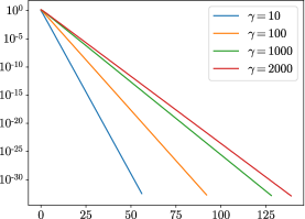
Figure 1: The singular values $\alpha_{n}$ of $T_{\gamma}$, as a function of $n$

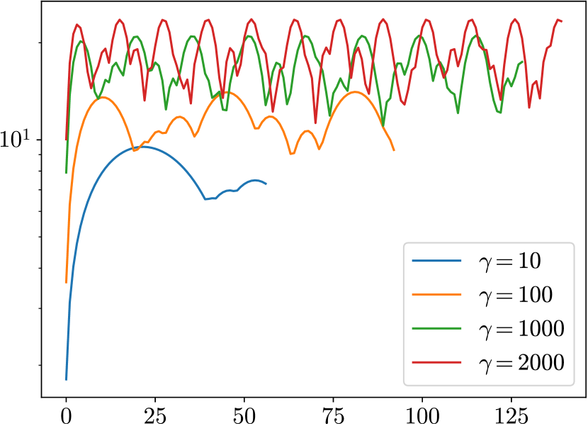
(a) ${\lVert u_{n}\rVert}_{L^{\infty}[a,b]}$, as a function of $n$

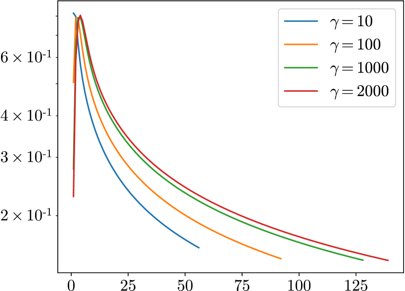
(b) ${\lVert\widetilde{w}\rVert}_{2}$ corresponding to $n$

Figure 2:

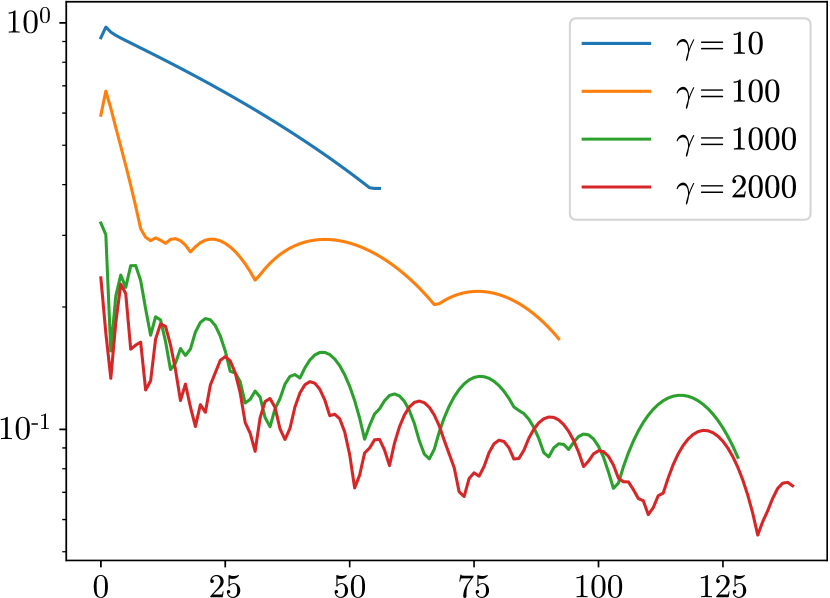
(a) ${\lVert v_{n}\rVert}_{L^{\infty}[0,\infty)}$, as a function of $n$

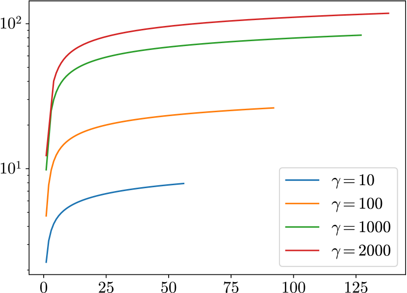
(b) $\max_{j}{\sqrt{w_{j}}}$ corresponding to $n$

Figure 3:

4 Analytical Apparatus

In this section, we present the principal analytical tools of this paper.

The following theorem states that the product of any two functions in the range of the operator $T_{\gamma}$, introduced in Section 2.1, can be expressed as a function in the range of $T_{\gamma}$, after a change of variable.

Theorem 4.1.

Suppose that the functions $p$, $q$ $\in L^{2}[0,\infty)$ are defined by

$$p(x)=\int_{0}^{1}e^{-x(t+\frac{1}{\gamma-1})}\eta(t)\,dt,$$ (36)

and

$$q(x)=\int_{0}^{1}e^{-x(t+\frac{1}{\gamma-1})}\varphi(t)\,dt,$$ (37)

respectively, for some $\eta$, $\varphi$ $\in L^{2}[0,1]$, and some $\gamma>1$. Then, there exists a $\sigma\in L^{2}[0,1]$, such that

$$p(x)\cdot q(x)=\int_{0}^{1}e^{-x(2t+\frac{2}{\gamma-1})}\sigma(t)\,dt.$$ (38)

Proof. For any $p$ and $q$ defined by Equation 36 and Equation 37, we have

$$p(x)\cdot q(x) =\int_{0}^{1}e^{-x(t+\frac{1}{\gamma-1})}\eta(t)\,dt\int_{0}^{1}e^{-x(s+\frac{1}{\gamma-1})}\varphi(s)\,ds$$

$$=\int_{0}^{1}\int_{0}^{1}e^{-x(t+s+\frac{2}{\gamma-1})}\eta(t)\varphi(s)\,ds\,dt.$$ (39)

Defining a new variable $u=t+s$ and changing the range of integration, Section 4 becomes

$$p(x)\cdot q(x)=\int_{0}^{1}e^{-x(u+\frac{2}{\gamma-1})}\int_{0}^{u}\eta(u-s)\varphi(s)\,ds\,du$$

$$\hskip 99.58464pt+\int_{1}^{2}e^{-x(u+\frac{2}{\gamma-1})}\int_{u-1}^{1}\eta(u-s)\varphi(s)\,ds\,du.$$ (40)

Letting $v=\frac{u}{2}$, we have

$$p(x)\cdot q(x)=\int_{0}^{\frac{1}{2}}e^{-x(2v+\frac{2}{\gamma-1})}\int_{0}^{2v}\eta(2v-s)\varphi(s)\,ds\,2dv$$

$$\hskip 99.58464pt+\int_{\frac{1}{2}}^{1}e^{-x(2v+\frac{2}{\gamma-1})}\int_{2v-1}^{1}\eta(2v-s)\varphi(s)\,ds\,2dv$$

$$\hskip 39.83385pt=\int_{0}^{1}e^{-x(2v+\frac{2}{\gamma-1})}\sigma(v)\,dv,$$ (41)

where

$$\sigma(v) =2\int_{0}^{2v}\eta(2v-s)\varphi(s)\,ds,$$ (42)

for $v\in[0,\frac{1}{2}]$, and

$$\sigma(v) =2\int_{2v-1}^{1}\eta(2v-s)\varphi(s)\,ds,$$ (43)

for $v\in[\frac{1}{2},1]$. $\blacksquare$

Observation 4.1.

Suppose we have nodes $x_{1}$, $x_{2}$, …, $x_{n}$ and weights $w_{1}$, $w_{2}$, …, $w_{n}$, such that

$$\Bigl{|}\int_{0}^{\infty}\int_{0}^{1}e^{-x(t+\frac{1}{\gamma-1})}\eta(t)\,dt\,dx-\sum_{j=1}^{n}w_{j}\int_{0}^{1}e^{-x_{j}(t+\frac{1}{\gamma-1})}\eta(t)\,dt\Bigr{|}\leq\epsilon{\lVert\eta\rVert}_{L^{2}[0,1]},$$ (44)

for any $\eta$ $\in L^{2}[0,1]$. Notice that

$$\hskip 42.67912pt\int_{0}^{\infty}p(x)\cdot q(x)\,dx$$

$$\hskip 28.45274pt=\int_{0}^{\infty}p(\frac{u}{2})\cdot q(\frac{{u}}{2})\cdot\frac{1}{2}\,du$$

$$\hskip 28.45274pt=\int_{0}^{\infty}\frac{1}{2}\int_{0}^{1}e^{-u(t+\frac{1}{\gamma-1})}\sigma(t)\,dt\,du.$$ (45)

Thus,

$$\Bigl{|}\int_{0}^{\infty}p(x)\cdot q(x)\,dx-\sum_{j=1}^{n}\frac{w_{j}}{2}\cdot p(\frac{x_{j}}{2})\cdot q(\frac{x_{j}}{2})\Bigr{|}\leq\frac{1}{2}\epsilon{\lVert\sigma\rVert}_{L^{2}[0,1]}\leq\epsilon{\lVert\eta\rVert}_{L^{2}[0,1]}{\lVert\varphi\rVert}_{L^{2}[0,1]}.$$ (46)

The following theorem shows that the product of any two functions in the range of $T^{*}_{\gamma}$, can be expressed as a function in the range of $T^{*}_{\gamma}$.

Theorem 4.2.

Suppose that the functions $p,q\in L^{2}[0,1]$ are defined by

$$p(t)=\int_{0}^{\infty}e^{-x(t+\frac{1}{\gamma-1})}\eta(x)\,dx,$$ (47)

and

$$q(t)=\int_{0}^{\infty}e^{-x(t+\frac{1}{\gamma-1})}\varphi(x)\,dx,$$ (48)

respectively, for some $\eta$, $\varphi\in L^{2}[0,\infty)$, and some $\gamma>1$. Then, there exists a $\sigma\in L^{2}[0,\infty)$, such that

$$p(t)\cdot q(t)=\int_{0}^{\infty}e^{-x(t+\frac{1}{\gamma-1})}\sigma(x)\,dx.$$ (49)

Proof. For any $p$ and $q$ defined by Equation 47 and Equation 48, we have

$$p(t)\cdot q(t) =\int_{0}^{\infty}e^{-\omega(t+\frac{1}{\gamma-1})}\eta(\omega)\,d\omega\int_{0}^{\infty}e^{-x(t+\frac{1}{\gamma-1})}\varphi(x)\,dx$$

$$=\int_{0}^{\infty}\int_{0}^{\infty}e^{-(\omega+x)(t+\frac{1}{\gamma-1})}\eta(\omega)\varphi(x)\,dx\,d\omega.$$ (50)

Defining $u=\omega+x$ and changing the range of integration, 7 becomes

$$p(t)\cdot q(t) =\int_{0}^{\infty}e^{-u(t+\frac{1}{\gamma-1})}\int_{0}^{u}\eta(\omega)\varphi(u-\omega)\,d\omega\,du$$

$$=\int_{0}^{\infty}e^{-u(t+\frac{1}{\gamma-1})}\sigma(u)\,du,$$ (51)

where

$$\sigma(u)=\int_{0}^{u}\eta(\omega)\varphi(u-\omega)\,d\omega,$$ (52)

for $u\in[0,\infty)$. $\blacksquare$

Observation 4.2.

Suppose we have nodes $t_{1}$, $t_{2}$, …, $t_{n}$ and weights $w_{1}$, $w_{2}$, …, $w_{n}$, such that

$$\Bigl{|}\int_{0}^{1}\int_{0}^{\infty}e^{-x(t+\frac{1}{\gamma-1})}\eta(x)\,dx\,dt-\sum_{j=1}^{n}w_{j}\int_{0}^{\infty}e^{-x(t_{j}+\frac{1}{\gamma-1})}\eta(x)\,dx\Bigr{|}\leq\epsilon{\lVert\eta\rVert}_{L^{2}[0,\infty)},$$ (53)

for any $\eta$ $\in L^{2}[0,\infty)$. Since $p(t)\cdot q(t)$ is in the range of $T^{*}_{\gamma}$, we have

$$\Bigl{|}\int_{0}^{1}p(t)\cdot q(t)\,dt-\sum_{j=1}^{n}w_{j}\cdot p(t_{j})\cdot q({t_{j}})\Bigr{|}\leq\epsilon{\lVert\sigma\rVert}_{L^{2}[0,\infty)}\leq\epsilon{\lVert\eta\rVert}_{L^{2}[0,\infty)}{\lVert\varphi\rVert}_{L^{2}[0,\infty)}.$$ (54)

Leveraging the multiplication rule established earlier, we demonstrate that the following quadrature rule accurately integrates the products of the kernel of $T_{\gamma}$ and the right singular functions of $T_{\gamma}$.

Corollary 4.3.

Suppose that we have a quadrature rule to integrate $\alpha_{i}u_{i}\cdot\alpha_{j}u_{j}$ to within an error of $\epsilon$, for all $i,j=0$, $1$, …, $n-1$. Suppose further that $t_{1}$, $t_{2}$, …, $t_{m}$ are the quadrature nodes, and $w_{1}$, $w_{2}$, …, $w_{m}$ are the quadrature weights. Then, the error of the quadrature rule applied to functions of the form $f(t)=e^{-x(t+\frac{1}{\gamma-1})}u_{i}(t)$, with $x\in[0,\infty)$, is roughly equal to

$$\frac{\epsilon}{\alpha_{i}}\sum_{j=0}^{n-1}{\lVert v_{j}\rVert}_{L^{\infty}[0,\infty)}+\alpha_{n}\cdot{\lVert v_{n}\rVert}_{L^{\infty}[0,\infty)}\cdot{\lVert u_{n}\rVert}_{L^{\infty}[0,1]}\cdot{\lVert u_{i}\rVert}_{L^{\infty}[0,1]}\cdot\sum_{k=1}^{m}|w_{k}|.$$ (55)

Proof. Since $e^{-x(t+\frac{1}{\gamma-1})}$ can be written as

$$e^{-x(t+\frac{1}{\gamma-1})}=\sum_{i=0}^{\infty}v_{i}(x)\alpha_{i}u_{i}(t),$$ (56)

we have

$$\int_{0}^{1}e^{-x(t+\frac{1}{\gamma-1})}u_{i}(t)\,dt-\sum_{k=1}^{m}w_{k}e^{-x(t_{k}+\frac{1}{\gamma-1})}u_{i}(t_{k})$$

$$=\int_{0}^{1}\Bigl{(}\sum_{j=0}^{\infty}v_{j}(x)\alpha_{j}u_{j}(t)\Bigr{)}u_{i}(t)\,dt-\sum_{k=1}^{m}w_{k}\Bigl{(}\sum_{j=0}^{\infty}v_{j}(x)\alpha_{j}u_{j}(t_{k})\Bigr{)}u_{i}(t_{k})$$

$$=\int_{0}^{1}v_{i}(x)\alpha_{i}u^{2}_{i}(t)\,dt-\sum_{k=1}^{m}w_{k}\Bigl{(}\sum_{j=0}^{\infty}v_{j}(x)\alpha_{j}u_{j}(t_{k})\Bigr{)}u_{i}(t_{k})$$

$$=\int_{0}^{1}v_{i}(x)\alpha_{i}u^{2}_{i}(t)\,dt-\Bigl{(}\sum_{j=0}^{n-1}\int_{0}^{1}v_{j}(x)\alpha_{j}u_{j}(t)u_{i}(t)\,dt+\sum_{j=0}^{n-1}v_{j}(x)\alpha_{j}\Bigl{(}\frac{\epsilon}{\alpha_{i}\alpha_{j}}\Bigr{)}$$

$$\hskip 14.22636pt+\sum_{j=n}^{\infty}\sum_{k=1}^{m}w_{k}v_{j}(x)\alpha_{j}u_{j}(t_{k})u_{i}(t_{k})\Bigr{)}$$

$$=-\Bigl{(}\sum_{j=0}^{n-1}v_{j}(x)\alpha_{j}\Bigl{(}\frac{\epsilon}{\alpha_{i}\alpha_{j}}\Bigr{)}+\sum_{j=n}^{\infty}\sum_{k=1}^{m}w_{k}v_{j}(x)\alpha_{j}u_{j}(t_{k})u_{i}(t_{k})\Bigr{)}$$

$$=-\Bigl{(}\sum_{j=0}^{n-1}v_{j}(x)\frac{\epsilon}{\alpha_{i}}+\sum_{j=n}^{\infty}\sum_{k=1}^{m}w_{k}v_{j}(x)\alpha_{j}u_{j}(t_{k})u_{i}(t_{k})\Bigr{)}.$$ (57)

Since $\{\alpha_{i}\}_{i=0,1,\ldots,\infty}$ decays exponentially, we have

$$\Bigl{|}\int_{0}^{1}e^{-x(t+\frac{1}{\gamma-1})}u_{i}(t)\,dt-\sum_{k=1}^{m}w_{k}e^{-x(t_{k}+\frac{1}{\gamma-1})}u_{i}(t_{k})\Bigr{|}$$

$$\approx\Bigl{|}\sum_{j=0}^{n-1}v_{j}(x)\frac{\epsilon}{\alpha_{i}}+\sum_{k=1}^{m}w_{k}v_{n}(x)\alpha_{n}u_{n}(t_{k})u_{i}(t_{k})\Bigr{|}$$

$$\leq\frac{\epsilon}{\alpha_{i}}\sum_{j=0}^{n-1}{\lVert v_{j}\rVert}_{L^{\infty}[0,\infty)}+\sum_{k=1}^{m}|w_{k}|\cdot\alpha_{n}\cdot{\lVert v_{n}\rVert}_{L^{\infty}[0,\infty)}\cdot|u_{n}(t_{k})|\cdot|u_{i}(t_{k})|$$

$$\leq\frac{\epsilon}{\alpha_{i}}\sum_{j=0}^{n-1}{\lVert v_{j}\rVert}_{L^{\infty}[0,\infty)}+\alpha_{n}\cdot{\lVert v_{n}\rVert}_{L^{\infty}[0,\infty)}\cdot{\lVert u_{n}\rVert}_{L^{\infty}[0,1]}\cdot{\lVert u_{i}\rVert}_{L^{\infty}[0,1]}\cdot\sum_{k=1}^{m}|w_{k}|.$$ (58)

$\blacksquare$

Suppose that $x_{1}$, $x_{2}$, …, $x_{m}$ and $w_{1}$, $w_{2}$, …, $w_{m}$ are the nodes and weights of a quadrature rule which integrates $\alpha_{i}v_{i}\cdot\alpha_{j}v_{j}$, to within an error of $\epsilon$, for all $i,j=0$, $1$, …, $n-1$. The following theorem shows that, if the left singular functions $\{v_{i}\}_{i=0,1,\ldots,n-1}$ of the operator $T_{\gamma}$, are used as interpolation basis, then, the interpolation matrix for the nodes $x_{1}$, $x_{2}$, …, $x_{m}$ is well conditioned, provided that the maximum error $\epsilon$ of integrating $\alpha_{i}v_{i}\cdot\alpha_{j}v_{j}$, for $i,j=0$, $1$, …, $n-1$, is sufficiently small.

Theorem 4.4.

Suppose that we have an $m$-point quadrature rule which integrates $\alpha_{i}v_{i}\cdot\alpha_{j}v_{j}$, to within an error of $\epsilon$, for all $i,j$ $=0$, $1$, …, $n-1$. Suppose further that $x_{1}$, $x_{2}$, …, $x_{m}$ are the quadrature nodes, and $w_{1}$, $w_{2}$, …, $w_{m}$ are the quadrature weights. Let the matrix $A\in\mathbb{R}^{m\times n}$ be given by the formula

$$A=\begin{pmatrix}v_{0}(x_{1})&v_{1}(x_{1})&\ \ldots&\ v_{n-1}(x_{1})\\ v_{0}(x_{2})&v_{1}(x_{2})&\ \ldots&\ v_{n-1}(x_{2})\\ \vdots&\vdots&\ \ddots&\vdots\\ v_{0}(x_{m})&v_{1}(x_{m})&\ \ldots&\ v_{n-1}(x_{m})\end{pmatrix},$$ (59)

and let the matrix $W$ be the diagonal matrix with diagonal entries $w_{1}$, $w_{2}$, …, $w_{m}$. We define the matrix $E=[e_{jk}]$ such that

$$E=I-A^{T}WA.$$ (60)

Then,

$$|e_{jk}|\leq\frac{\epsilon}{\alpha_{j-1}\alpha_{k-1}}.$$ (61)

Proof. From Equation 60, we have

$$e_{jk}=\delta_{jk}-\sum_{l=1}^{m}w_{l}v_{j-1}(x_{l})v_{k-1}(x_{l}),$$ (62)

where $\delta_{jk}=1$ if $j=k$, and $\delta_{jk}=0$ otherwise. Then,

$$|e_{jk}|=\Bigl{|}\delta_{jk}-\sum_{l=1}^{m}w_{l}\alpha_{j-1}v_{j-1}(x_{l})\cdot\alpha_{k-1}v_{k-1}(x_{l})\frac{1}{\alpha_{j-1}\alpha_{k-1}}\Bigr{|}$$

$$\hskip 2.84526pt\leq\Bigl{|}\delta_{jk}-\frac{1}{\alpha_{j-1}\alpha_{k-1}}\int_{0}^{\infty}\alpha_{j-1}v_{j-1}(x)\cdot\alpha_{k-1}v_{k-1}(x)\,dx\Bigr{|}+\frac{\epsilon}{\alpha_{j-1}\alpha_{k-1}}$$

$$\hskip 2.84526pt=\frac{\epsilon}{\alpha_{j-1}\alpha_{k-1}}.$$ (63)

$\blacksquare$

The following corollary establishes an upper bound on the norm of the pseudo-inverse $A^{\dagger}$ of the matrix $A$ defined in Equation 59.

Corollary 4.5.

Suppose that we have a collection of quadrature nodes $x_{1}$, $x_{2}$, …, $x_{m}$ and positive quadrature weights $w_{1}$, $w_{2}$, …, $w_{m}$, which integrates $\alpha_{i}v_{i}\cdot\alpha_{j}v_{j}$ to within an error of $\epsilon\leq\frac{\alpha_{n}^{2}}{2\sqrt{n}}$, for all $i,j$ $=0$, $1$, …, $n-1$. Let $A\in\mathbb{R}^{m\times n}$ be the matrix defined in Equation 59. Then,

$${\lVert A^{\dagger}\rVert}_{2} <\sqrt{2}\max_{1\leq i\leq m}\sqrt{w_{i}},$$ (64)

where $A^{\dagger}\in\mathbb{R}^{n\times m}$ is the pseudo-inverse of $A$.

Proof. Recalling that $w_{1}$, $w_{2}$, …, $w_{m}$ are positive, we let $W^{\frac{1}{2}}$ denote a diagonal matrix with entries $\sqrt{w_{1}}$, $\sqrt{w_{2}}$, …, $\sqrt{w_{m}}$. We define $B$ such that $B=W^{\frac{1}{2}}A$. It follows from Equation 60 that $B^{T}B=I-E$. Since $e_{jk}<\frac{\epsilon}{\alpha_{n}^{2}}$, for all $j,k=1$, $2$, …, $n$, we have ${\lVert E\rVert}_{2}<\frac{\epsilon}{\alpha_{n}^{2}}\sqrt{n}$. Let $\widetilde{\sigma}_{1}$, $\widetilde{\sigma}_{2}$, …, $\widetilde{\sigma}_{n}$ denote the singular values of $B^{T}B$. Then, it can be shown that (see Theorem IIIa in [2])

$$|\widetilde{\sigma}_{j}-1|\leq{\lVert E\rVert}_{2}<\frac{\epsilon}{\alpha_{n}^{2}}\sqrt{n},$$ (65)

for all $j=1$, $2$, …, $n$. This means that

$$1-\frac{\epsilon}{\alpha_{n}^{2}}\sqrt{n}<\widetilde{\sigma}_{j}<1+\frac{\epsilon}{\alpha_{n}^{2}}\sqrt{n}.$$ (66)

Letting $k=\min\{n,m\}$ and $\sigma_{1}$, $\sigma_{2}$, …, $\sigma_{k}$ be the singular values of $B$, we have

$$\sqrt{1-\frac{\epsilon}{\alpha_{n}^{2}}\sqrt{n}}<{\sigma}_{j}<\sqrt{1+\frac{\epsilon}{\alpha_{n}^{2}}\sqrt{n}}.$$ (67)

Letting $B^{\dagger}$ be the pseudo-inverse of $B$, such that $B^{\dagger}B=I$, since $B=W^{\frac{1}{2}}A$, we have that $A^{\dagger}=B^{\dagger}W^{\frac{1}{2}}$. Thus,

$${\lVert A^{\dagger}\rVert}_{2} \leq{\lVert B^{\dagger}\rVert}_{2}{\lVert W^{\frac{1}{2}}\rVert}_{2}$$

$$<\frac{1}{\sqrt{1-\frac{\epsilon}{\alpha_{n}^{2}}\sqrt{n}}}\cdot\max_{1\leq i\leq m}\sqrt{w_{i}}.$$ (68)

If we have $\epsilon\leq\frac{\alpha_{n}^{2}}{2\sqrt{n}}$, then 10 implies that

$${\lVert A^{\dagger}\rVert}_{2} <\sqrt{2}\max_{1\leq i\leq m}\sqrt{w_{i}}.$$ (69)

$\blacksquare$

5 Selecting the Quadrature Nodes and Weights

In this section, we discuss how to construct the quadrature rules described in the conditions of the theorems presented in Section 4.

Suppose that the nodes $t_{1}$, $t_{2}$, …, $t_{m}$ are the roots of $u_{m}(t)$, and that the weights $\widetilde{w}_{1}$, $\widetilde{w}_{2}$, …, $\widetilde{w}_{m}$ satisfy

$$\int_{0}^{1}u_{i}(t)\,dt=\sum_{k=1}^{m}\widetilde{w}_{k}u_{i}(t_{k}),$$ (70)

for all $i=0$, $1$, …, $m-1$. Then,

$$\Bigl{|}\int_{0}^{1}\alpha_{i}u_{i}(t)dt-\sum_{k=1}^{m}\widetilde{w}_{k}\alpha_{i}u_{i}(t_{k})\Bigr{|}\leq\mathds{1}_{\{i\geq m\}}\alpha_{i}{\lVert u_{i}\rVert}_{L^{\infty}[0,1]}(1+{\lVert\widetilde{w}\rVert}_{1})\lesssim\alpha_{m},$$ (71)

from which it follows that

$$\Bigl{|}\int_{0}^{1}\int_{0}^{\infty}e^{-x(t+\frac{1}{\gamma-1})}\eta(x)\,dx\,dt-\sum_{j=1}^{n}\widetilde{w}_{k}\int_{0}^{\infty}e^{-x(t_{k}+\frac{1}{\gamma-1})}\eta(x)\,dx\Bigr{|}\lesssim\alpha_{m}{\lVert\eta\rVert}_{L^{2}[0,\infty)}.$$ (72)

4.2 implies that

$$E_{1}:=\max_{0\leq i,j\leq n-1}{\Bigl{|}\int_{0}^{1}\alpha_{i}u_{i}(t)\cdot\alpha_{j}u_{j}(t)\,dt-\sum_{k=1}^{m}\widetilde{w}_{k}\alpha_{i}u_{i}(t_{k})\cdot\alpha_{j}u_{j}(t_{k})\Bigr{|}}\lesssim\alpha_{m}.$$ (73)

If $E_{1}\leq\alpha^{2}_{n}$, then Corollary 4.3 guarantees that such a quadrature rule integrates the functions $f(t)=e^{-x(t+\frac{1}{\gamma-1})}u_{i}(t)$, for $i=0$, $1$, …, $n-1$, to an error of approximately the same size as $\alpha_{n}$. Since the singular values $\alpha_{i}$ decay exponentially, we see that $E_{1}\lesssim\alpha_{m}\leq\alpha^{2}_{n}$ when $m\approx 2n$. In practice, however, it is unnecessary to take $m$ to be so large. Numerical experiments for $\gamma=10$, $50$ and $250$ demonstrate that, by choosing $m=n$, the error of the quadrature rule applied to $\alpha_{i}u_{i}\cdot\alpha_{j}u_{j}$, for all $i,j=0$, $1$, …, $n-1$, turns out to be smaller than $\alpha^{2}_{n}$, as shown in Figures 4(a), 5(a) and 6(a). Thus, it follows from Corollary 4.3 that the error of the quadrature rule applied to $f(t)=e^{-x(t+\frac{1}{\gamma-1})}u_{i}(t)$, for $i=0$, $1$, …, $n-1$, is approximately $\alpha_{n}$.

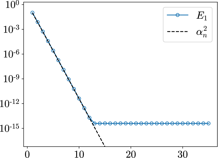
(a) A comparison between $E_{1}$ and $\alpha^{2}_{n}$, as a function of $n$.

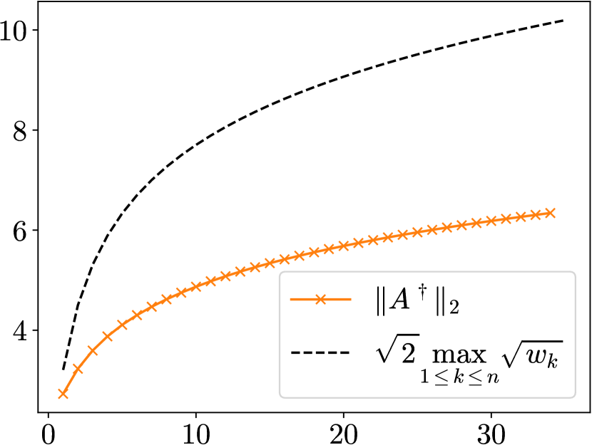
(b) A comparison between ${\lVert A^{\dagger}\rVert}_{2}$ and $\sqrt{2}\max_{k}\sqrt{w_{k}}$, as a function of $n$.

Figure 4: $\gamma=10$

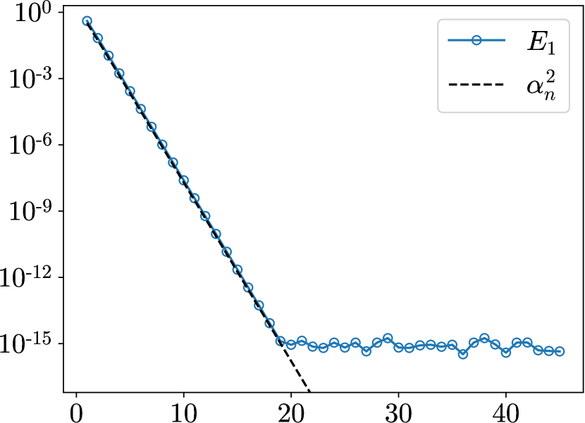
(a) A comparison between $E_{1}$ and $\alpha^{2}_{n}$, as a function of $n$.

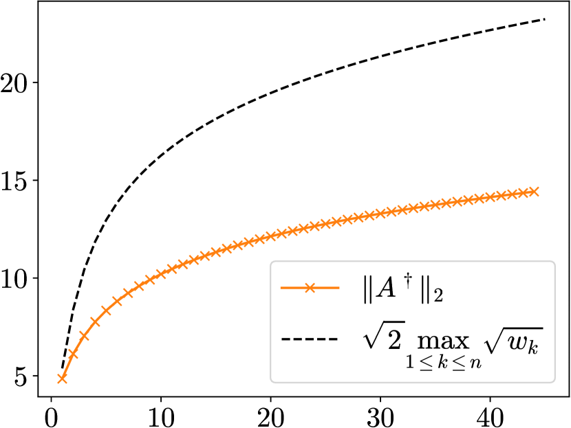
(b) A comparison between ${\lVert A^{\dagger}\rVert}_{2}$ and $\sqrt{2}\max_{k}\sqrt{w_{k}}$, as a function of $n$.

Figure 5: $\gamma=50$

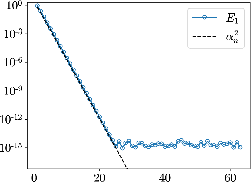
(a) A comparison between $E_{1}$ and $\alpha^{2}_{n}$, as a function of $n$.

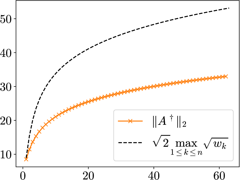
(b) A comparison between ${\lVert A^{\dagger}\rVert}_{2}$ and $\sqrt{2}\max_{k}\sqrt{w_{k}}$, as a function of $n$.

Figure 6: $\gamma=250$

Suppose now that the nodes $x_{1}$, $x_{2}$, …, $x_{m}$ are the roots of $v_{m}(x)$, and the weights $w_{1}$, $w_{2}$, …, $w_{m}$ satisfy

$$\int_{0}^{\infty}v_{i}(x)\,dx=\sum_{k=1}^{m}{w}_{k}v_{i}(x_{k}),$$ (74)

for all $i=0$, $1$, …, $m-1$. Since

$$\Bigl{|}\int_{0}^{\infty}\alpha_{i}v_{i}(t)dx-\sum_{k=1}^{m}{w}_{k}\alpha_{i}v_{i}(x_{k})\Bigr{|}\leq\mathds{1}_{\{i\geq m\}}\alpha_{i}({\lVert v_{i}\rVert}_{L^{1}[0,\infty)}+{\lVert v_{i}\rVert}_{L^{\infty}[0,\infty)}{\lVert w\rVert}_{1})\lesssim\alpha_{m},$$ (75)

it follows that

$$\Bigl{|}\int_{0}^{\infty}\int_{0}^{1}e^{-x(t+\frac{1}{\gamma-1})}\eta(t)\,dt\,dx-\sum_{j=1}^{n}w_{k}\int_{0}^{1}e^{-x_{k}(t+\frac{1}{\gamma-1})}\eta(t)\,dt\Bigr{|}\lesssim\alpha_{m}{\lVert\eta\rVert}_{L^{2}[0,1]}.$$ (76)

4.1 implies that

$$E_{2}:=\max_{0\leq i,j\leq n-1}\Bigl{|}\int_{0}^{\infty}\alpha_{i}v_{i}(x)\cdot\alpha_{j}v_{j}(x)\,dx-\sum_{k=1}^{m}\frac{{w}_{k}}{2}\alpha_{i}v_{i}(\frac{x_{k}}{2})\cdot\alpha_{j}v_{j}(\frac{x_{k}}{2})\Bigr{|}\lesssim\alpha_{m}.$$ (77)

If $E_{2}\leq\frac{\alpha^{2}_{n}}{a\sqrt{n}}$, then Corollary 4.5 guarantees that the norm of $A^{\dagger}\in\mathbb{R}^{n\times m}$ achieves the bound specified in Equation 64. We see that $E_{2}\lesssim\alpha_{m}\leq\frac{\alpha^{2}_{n}}{a\sqrt{n}}$ when $m\approx 2n$. However, instead of choosing $m$ to be so large, we can once again take $m=n$ and use the nodes $x_{k}$ rather than $x_{k}/2$. Unlike the error of the quadrature rule in Equation 70 applied to $\alpha_{i}u_{i}\cdot\alpha_{j}u_{j}$, for $i,j=0$, $1$, …, $n-1$, which is, in practice, less than $\alpha^{2}_{n}$, the error of the quadrature rule in Equation 74 applied to $\alpha_{i}v_{i}\cdot\alpha_{j}v_{j}$, for $i,j=0$, $1$, …, $n-1$, lies somewhere between $\alpha^{2}_{n}$ and $\alpha_{n}$. However, we observe that the special structure of $A\in\mathbb{R}^{n\times n}$ allows the norm of $A^{\dagger}$ to still attain the bound specified in Equation 64. The results for $\gamma=10$, $50$ and $250$ are shown in Figures 4(b), 5(b) and 6(b), respectively.

Remark 5.1.

It is worth emphasizing that the choice of quadrature nodes is not unique. Any set of quadrature nodes with corresponding weights that satisfy Equation 70 or Equation 74 can be employed for our purposes. In this paper, we choose the roots of $u_{m}$ and $v_{m}$ to be the quadrature nodes, since the associated weights are positive and reasonably small, which we have shown in Section 3.

6 Approximation by Singular Powers

In this section, we present a method for approximating a function of the form

$$f(x)=\int_{a}^{b}x^{\mu}\sigma(\mu)\,d\mu,\qquad x\in[0,1],$$ (78)

for some signed Radon measure $\sigma(\mu)$, using a basis of $\{x^{t_{j}}\}_{j=1}^{N}$ for some specially chosen points $t_{1}$, $t_{2}$, …, $t_{N}\in[a,b]$. Our approach involves approximating $f$ by the left singular functions of $T_{\gamma}$, and then discretizing the integral representation of these left singular functions in the form of $\{x^{t_{j}}\}_{j=1}^{N}$.

In the following theorem, we establish the existence of such an approximation, and quantify its approximation error.

Theorem 6.1.

Let $f$ be a function of the form Equation 78. Suppose that $\widetilde{t}_{1}$, $\widetilde{t}_{2}$, …, $\widetilde{t}_{N}$ and $\widetilde{w}_{1}$, $\widetilde{w}_{2}$, …, $\widetilde{w}_{N}$ are the quadrature nodes and weights of a quadrature rule such that $E_{1}\leq\alpha^{2}_{n}$, where $E_{1}$ is defined in Equation 73. Let $t_{j}=a+(b-a)\widetilde{t}_{j}$, for all $j=1$, $2$, …, $N$. Then, there exists a vector $c\in\mathbb{R}^{N}$ such that the function

$${f}_{N}(x)=\sum_{j=1}^{N}c_{j}x^{t_{j}},$$ (79)

satisfies

$${\lVert f-f_{N}\rVert}_{L^{\infty}[0,1]}\leq\alpha_{n}\cdot{\lVert\sigma\rVert}_{L^{1}[a,b]}\cdot\bigl{(}{\lVert u_{n}\rVert}_{L^{\infty}[0,1]}\cdot{\lVert v_{n}\rVert}_{L^{\infty}[0,\infty)}$$

$$\hskip 113.81102pt+{n}\max_{0\leq i\leq n-1}{\lVert u_{i}\rVert}_{L^{\infty}[0,1]}\cdot\frac{\max_{0\leq i\leq n-1}\widetilde{E}_{i}}{\alpha_{n}}\bigr{)},$$ (80)

where

$$\widetilde{E}_{i}\leq\alpha_{n}\sum_{j=0}^{n-1}{\lVert v_{j}\rVert}_{L^{\infty}[0,\infty)}+\alpha_{n}\cdot{\lVert v_{n}\rVert}_{L^{\infty}[0,\infty)}\cdot{\lVert u_{n}\rVert}_{L^{\infty}[0,1]}\cdot{\lVert u_{i}\rVert}_{L^{\infty}[0,1]}\cdot\sum_{l=1}^{N}|\widetilde{w}_{l}|\approx\alpha_{n},$$ (81)

and the norm of the coefficient vector $c$ is bounded by

$${\lVert{{c}}\rVert}_{2}\leq\sqrt{\sum_{j=1}^{N}|\widetilde{w}_{j}|^{2}}\cdot\sqrt{N}{n}\cdot|{\sigma}|\cdot\bigl{(}\max_{0\leq i\leq n-1}{\lVert u_{i}\rVert}_{L^{\infty}[0,1]}\bigr{)}^{2}.$$ (82)

Proof. Substituting $\omega=-\log{x}$ into Equation 78, we have

$$f(e^{-\omega}) =\int_{a}^{b}e^{-\omega\mu}\sigma(\mu)\,d\mu,$$

$$=\int_{0}^{1}e^{-\widetilde{\omega}(\bar{\mu}+\frac{1}{\gamma-1})}{(b-a)}\sigma((b-a)\bar{\mu}+a)\,d\bar{\mu},\qquad\widetilde{\omega}\in[0,\infty),$$ (83)

where $\bar{\mu}=\frac{\mu-a}{b-a}$, and $\widetilde{\omega}=(b-a)\omega$. Since $\{\alpha_{i}\}_{i=0,1,\ldots,\infty}$ decays exponentially, we truncate the SVD of the operator $T_{\gamma}$ after $n$ terms and obtain

$$e^{-\omega(t+\frac{1}{\gamma-1})} =\sum_{i=0}^{\infty}v_{i}(\omega)\alpha_{i}u_{i}(t)\approx\sum_{i=0}^{n-1}v_{i}(\omega)\alpha_{i}u_{i}(t).$$ (84)

Then, we construct the approximation $\widetilde{f}$ to $f$, defined by

$$\widetilde{f}(e^{-{\widetilde{\omega}}})=\sum_{i=0}^{n-1}\alpha_{i}\biggl{(}\int_{0}^{1}u_{i}(\bar{\mu}){(b-a)}\sigma((b-a)\bar{\mu}+a)\,d\bar{\mu}\biggr{)}v_{i}(\widetilde{\omega}).$$ (85)

Thus,

$$\widetilde{f}(x) =\sum_{i=0}^{n-1}\alpha_{i}\biggl{(}\int_{0}^{1}u_{i}(\bar{\mu}){(b-a)}\sigma((b-a)\bar{\mu}+a)\,d\bar{\mu}\biggr{)}v_{i}(-(b-a)\log x)$$

$$=\sum_{i=0}^{n-1}\widetilde{c}_{i}\alpha_{i}v_{i}(-(b-a)\log x),$$ (86)

for $x\in[0,1]$, where

$$\widetilde{c}_{i}=\int_{0}^{1}u_{i}(\bar{\mu})(b-a)\sigma((b-a)\bar{\mu}+a)\,d\bar{\mu},$$ (87)

for $i=0$, $1$, …, $n-1$. We observe that

$$|\widetilde{c_{i}}|\leq|{\sigma}|\cdot{\lVert u_{i}\rVert}_{L^{\infty}[0,1]},$$ (88)

and

$${\lVert\widetilde{c}\rVert}_{2}\leq\sqrt{n}|{\sigma}|\cdot\max_{0\leq i\leq n-1}{\lVert u_{i}\rVert}_{L^{\infty}[0,1]}.$$ (89)

Thus,

$${\lVert f-\widetilde{f}\rVert}_{L^{\infty}[0,1]} ={\biggl{\lVert}\sum_{i=n}^{\infty}\widetilde{c}_{i}{\alpha}_{i}v_{i}(-(b-a)\log{x})\biggr{\rVert}}_{L^{\infty}[0,1]}$$

$$\approx{\bigl{\lVert}\widetilde{c}_{n}{\alpha}_{n}v_{n}(-(b-a)\log{x})\bigr{\rVert}}_{L^{\infty}[0,1]}$$

$$\leq\alpha_{n}\cdot|{\sigma}|\cdot{\lVert u_{n}\rVert}_{L^{\infty}[0,1]}\cdot{\lVert v_{n}\rVert}_{L^{\infty}[0,\infty)}.$$ (90)

According to Equation 5, we have

$$\alpha_{i}v_{i}(\omega)=\int_{0}^{1}e^{-\omega(t+\frac{1}{\gamma-1})}u_{i}(t)\,dt.$$ (91)

Since

$$E_{1}=\max_{0\leq i,j\leq n-1}\Bigl{|}\int_{0}^{1}\alpha_{i}u_{i}(t)\alpha_{j}u_{j}(t)\,dt-\sum_{l=1}^{N}\widetilde{w}_{l}\alpha_{i}u_{i}(\widetilde{t}_{l})\alpha_{j}u_{j}(\widetilde{t}_{l})\Bigr{|}\leq{\alpha_{n}}^{2},$$ (92)

for all $i,j$ $=0$, $1$, …, $n-1$, it follows from Corollary 4.3 that

$$\widetilde{E}_{i}:=\Bigl{|}\int_{0}^{1}e^{-\omega(t+\frac{1}{\gamma-1})}u_{i}(t)\,dt-\sum_{l=1}^{N}\widetilde{w}_{l}e^{-\omega(\widetilde{t}_{l}+\frac{1}{\gamma-1})}u_{i}(\widetilde{t}_{l})\Bigr{|}$$

$$\leq\alpha_{n}\sum_{j=0}^{n-1}{\lVert v_{j}\rVert}_{L^{\infty}[0,\infty)}+\alpha_{n}\cdot{\lVert v_{n}\rVert}_{L^{\infty}[0,\infty)}\cdot{\lVert u_{n}\rVert}_{L^{\infty}[0,1]}\cdot{\lVert u_{i}\rVert}_{L^{\infty}[0,1]}\cdot\sum_{l=1}^{N}|\widetilde{w}_{l}|.$$ (93)

Since $\sum_{l=1}^{N}|\widetilde{w}_{l}|$, ${\lVert v_{j}\rVert}_{L^{\infty}[0,\infty)}$ and ${\lVert u_{j}\rVert}_{L^{\infty}[0,1]}$ are small, for all $j=0$, $1$, …, $n-1$, as shown in Section 3, the discretization error, $\widetilde{E}_{i}$, is approximately of the size $\alpha_{n}$.

Recalling Section 6, we have

$$\widetilde{f}(x)=\sum_{i=0}^{n-1}\widetilde{c}_{i}\alpha_{i}v_{i}(-(b-a)\log x),$$ (94)

so

$$\Bigl{|}\widetilde{f}(e^{-\frac{\widetilde{\omega}}{b-a}})-\sum_{i=0}^{n-1}\widetilde{c}_{i}\sum_{j=1}^{N}\widetilde{w}_{j}e^{-\widetilde{\omega}(\widetilde{t}_{j}+\frac{1}{\gamma-1})}u_{i}(\widetilde{t}_{j})\Bigr{|}\leq\sum_{i=0}^{n-1}{\lvert\widetilde{c}_{i}\rvert}\widetilde{E}_{i},$$ (95)

which means that

$$\Bigl{|}\widetilde{f}(e^{-\frac{\widetilde{\omega}}{b-a}})-\sum_{i=0}^{n-1}\widetilde{c}_{i}\sum_{j=1}^{N}\widetilde{w}_{j}e^{-\widetilde{\omega}\bar{t}_{j}}u_{i}(\bar{t}_{j}-\frac{1}{\gamma-1})\Bigr{|}\leq\sum_{i=0}^{n-1}{\lvert\widetilde{c}_{i}\rvert}\widetilde{E}_{i},$$ (96)

where $\widetilde{\omega}=-(b-a)\log x$ and $\bar{t}_{j}=\widetilde{t}_{j}+\frac{1}{\gamma-1}$, for all $j=1$, $2$, …, $N$. Substituting $e^{-\frac{\widetilde{\omega}}{b-a}}=x$ into Equation 96, we define the approximation $f_{N}$ to $\widetilde{f}$,

$$f_{N}(x)=\sum_{i=0}^{n-1}\widetilde{c}_{i}\sum_{j=1}^{N}\widetilde{w}_{j}u_{i}(\bar{t}_{j}-\frac{1}{\gamma-1})x^{(b-a)\bar{t}_{j}},$$

$$\hskip 17.07164pt:=\sum_{j=1}^{N}{{c}}_{j}x^{(b-a)\bar{t}_{j}},\qquad x\in[0,1],$$ (97)

where ${{c}}_{j}=\widetilde{w}_{j}\sum_{i=0}^{n-1}\widetilde{c}_{i}u_{i}(\bar{t}_{j}-\frac{1}{\gamma-1})$, for $j=1$, $2$, …, $N$. Letting $t_{j}=(b-a)\bar{t}_{j}$, we have $t_{j}=(b-a)\widetilde{t}_{j}+a$, for $j=1$, $2$, …, $N$. Section 6 and Equation 89 imply that

$${\lVert{{c}}\rVert}_{2} \leq\sqrt{\sum_{j=1}^{N}|\widetilde{w}_{j}|^{2}}\cdot\sqrt{N}\sqrt{n}\cdot{\lVert\widetilde{c}\rVert}_{2}\max_{0\leq i\leq n-1}{\lVert u_{i}\rVert}_{L^{\infty}[0,1]}$$

$$\leq\sqrt{\sum_{j=1}^{N}|\widetilde{w}_{j}|^{2}}\cdot\sqrt{N}{n}\cdot|{\sigma}|\cdot\bigl{(}\max_{0\leq i\leq n-1}{\lVert u_{i}\rVert}_{L^{\infty}[0,1]}\bigr{)}^{2}.$$ (98)

The approximation error of $f_{N}$ to $\widetilde{f}$ can be bounded by

$${\lVert\widetilde{f}-{f}_{N}\rVert}_{L^{\infty}[0,1]}\leq{\sum_{i=0}^{n-1}{\lvert\widetilde{c}_{i}\rvert}\max_{0\leq i\leq n-1}\widetilde{E}_{i}}$$

$$\hskip 45.5244pt\leq\sqrt{n}{\lVert\widetilde{c}\rVert}_{2}\max_{0\leq i\leq n-1}\widetilde{E}_{i}$$

$$\hskip 45.5244pt\leq{n}|{\sigma}|\cdot\max_{0\leq i\leq n-1}{\lVert u_{i}\rVert}_{L^{\infty}[0,1]}\cdot\max_{0\leq i\leq n-1}\widetilde{E}_{i}.$$ (99)

Thus, we obtain the bound on the approximation error of $f_{N}$ to $f$ as

$${\lVert f-f_{N}\rVert}_{L^{\infty}[0,1]}\leq{\lVert f-\widetilde{f}\rVert}_{L^{\infty}[0,1]}+{\lVert\widetilde{f}-f_{N}\rVert}_{L^{\infty}[0,1]}$$

$$\hskip 51.21495pt\leq\alpha_{n}\cdot|{\sigma}|\cdot\bigl{(}{\lVert u_{n}\rVert}_{L^{\infty}[0,1]}\cdot{\lVert v_{n}\rVert}_{L^{\infty}[0,\infty)}$$

$$\hskip 113.81102pt+{n}\max_{0\leq i\leq n-1}{\lVert u_{i}\rVert}_{L^{\infty}[0,1]}\cdot\frac{\max_{0\leq i\leq n-1}\widetilde{E}_{i}}{\alpha_{n}}\bigr{)}.$$ (100)

$\blacksquare$

7 Numerical Algorithm and Error Analysis

In the previous section, we have shown that, given any function $f$ of the form Equation 78 and any quadrature rule such that $E_{1}\leq{\alpha_{n}}^{2}$, where $E_{1}$ is defined in Equation 73, there exists a coefficient vector $c\in\mathbb{R}^{N}$ such that, letting $t_{1}$, $t_{2}$, …, $t_{N}$ denote the quadrature nodes shifted to the interval $[a,b]$,

$${f}_{N}(x)=\sum_{j=1}^{N}c_{j}x^{t_{j}}$$ (101)

is uniformly close to $f$, to within an error given by Theorem 6.1.

In this section, we show that, by choosing a quadrature rule with quadrature nodes $s_{1}$, $s_{2}$, …, $s_{N}$ such that $E_{2}\leq\frac{{\alpha_{n}}^{2}}{2\sqrt{n}}$, where $E_{2}$ is defined in Equation 77, and letting

$$x_{j}=e^{-\frac{s_{j}}{b-a}},$$ (102)

for $j=1$, $2$, …, $N$, we can construct an approximation

$$\widehat{f}_{N}(x)=\sum_{j=1}^{N}\widehat{c}_{j}x^{t_{j}}$$ (103)

which is also uniformly close to $f$, by numerically solving a linear system

$$Vc=F,$$ (104)

for the coefficient vector $\widehat{c}\in\mathbb{R}^{N}$, where

$$V=\begin{pmatrix}x^{t_{1}}_{1}&x^{t_{2}}_{1}&\ \ldots&\ x^{t_{N}}_{1}\\ x^{t_{1}}_{2}&x^{t_{2}}_{2}&\ \ldots&\ x^{t_{N}}_{2}\\ \vdots&\vdots&\ \ddots&\vdots\\ x^{t_{1}}_{N}&x^{t_{2}}_{N}&\ \ldots&\ x^{t_{N}}_{N}\end{pmatrix}\in\mathbb{R}^{N\times N},$$ (105)

and

$$F=({f}(x_{1}),{f}(x_{2}),\ldots,{f}(x_{N}))^{T}\in\mathbb{R}^{N}.$$ (106)

The uniform approximation error of $\widehat{f}_{N}$ to $f$ over $[0,1]$ is bounded in Theorem 7.3. Recall that $E_{1}\leq\alpha^{2}_{n}$ and $E_{2}\leq\frac{{\alpha_{n}}^{2}}{2\sqrt{n}}$ when $N\approx 2n$ and the quadrature nodes are chosen to be the roots of $u_{N}(t)$ and $v_{N}(x)$ (see Section 5).

In the following lemma, we establish upper bounds on the norm and the residual of the perturbed TSVD solution $\widehat{c}$ to the linear system in Equation 104, in terms of the norm of the coefficient vector $c$ in Equation 101.

Lemma 7.1.

Let $V\in\mathbb{R}^{N\times N}$, $F\in\mathbb{R}^{N}$, and $\epsilon>0$. Suppose that

$$\widehat{c}_{k}=(V+\delta V)_{k}^{\dagger}(F+\delta F),$$ (107)

where $(V+\delta V)_{k}^{\dagger}$ is the pseudo-inverse of the $k$-TSVD of $V+\delta V$, so that

$$\widehat{\alpha}_{k}\geq\epsilon\geq\widehat{\alpha}_{k+1},$$ (108)

where $\widehat{\alpha}_{k}$ and $\widehat{\alpha}_{k+1}$ denote the $k$th and $(k+1)$th largest singular values of $V+\delta V$, where $\delta V\in\mathbb{R}^{N\times N}$ and $\delta F\in\mathbb{R}^{N}$, with

$${\lVert\delta V\rVert}_{2}\leq\epsilon_{0}\cdot\mu_{1}<\frac{\epsilon}{2},$$ (109)

and

$${\lVert\delta F\rVert}_{2}\leq\epsilon_{0}\cdot\mu_{2}.$$ (110)

Suppose further that

$$Vc=F+\Delta F,$$ (111)

for some $\Delta F\in\mathbb{R}^{N}$ and $c\in\mathbb{R}^{N}$. Then,

$${\lVert\widehat{c}_{k}\rVert}_{2}\leq\frac{1}{\widehat{\alpha}_{k}}(2\epsilon+\widehat{\alpha}_{k}){\lVert c\rVert}_{2}+\frac{1}{\widehat{\alpha}_{k}}({\lVert\Delta F\rVert}_{2}+\epsilon_{0}\cdot\mu_{2}),$$ (112)

and

$${\lVert V\widehat{c}_{k}-(F+\Delta F)\rVert}_{2} \leq 5\epsilon{\lVert c\rVert}_{2}+\frac{3}{2}{\lVert\Delta F\rVert}_{2}+\frac{3}{2}\epsilon_{0}\cdot\mu_{2}.$$ (113)

Proof. By Equation 107, we have

$$(V+\delta V)_{k}\widehat{c}_{k}=F+\delta F =F+\Delta F-\Delta F+\delta F=F+\Delta F+e,$$ (114)

where $e:=-\Delta F+\delta F$. Thus, Theorem 2.1 implies that

$${\lVert\widehat{c}_{k}\rVert}_{2} \leq\frac{1}{\widehat{\alpha}_{k}}(2\epsilon+\widehat{\alpha}_{k}){\lVert c\rVert}_{2}+\frac{1}{\widehat{\alpha}_{k}}{\lVert-\Delta F+\delta F\rVert}_{2}$$

$$\leq\frac{1}{\widehat{\alpha}_{k}}(2\epsilon+\widehat{\alpha}_{k}){\lVert c\rVert}_{2}+\frac{1}{\widehat{\alpha}_{k}}({\lVert\Delta F\rVert}_{2}+\epsilon_{0}\cdot\mu_{2}),$$ (115)

and that

$${\lVert V\widehat{c}_{k}-(F+\Delta F)\rVert}_{2} \leq 5\epsilon{\lVert c\rVert}_{2}+\frac{3}{2}{\lVert\Delta F\rVert}_{2}+\frac{3}{2}\epsilon_{0}\cdot\mu_{2}.$$ (116)

$\blacksquare$

The following observation bounds the backward error, ${\lVert V\widehat{c}_{k}-F\rVert}_{2}$, where $\widehat{c}_{k}$ is the TSVD solution to the perturbed linear system, defined in Equation 107.

Observation 7.1.

According to Lemma 7.1, the TSVD solution $\widehat{c}_{k}$ to the perturbed linear system is bounded by the norm of $c$, as described in Equation 112, where $c$ is the exact solution to the linear system $V{c}=F+\Delta F$, and satisfies Equation 82. Thus, the resulting backward error is bounded by

$${\lVert V\widehat{c}_{k}-F\rVert}_{2}={\bigl{\lVert}V\widehat{c}_{k}-\bigl{(}F+\Delta F\bigr{)}+\Delta F\bigr{\rVert}}_{2}$$

$$\hskip 19.91692pt\leq{\bigl{\lVert}V\widehat{c}_{k}-\bigl{(}F+\Delta F\bigr{)}\bigr{\rVert}}_{2}+{\lVert\Delta F\rVert}_{2}$$

$$\hskip 19.91692pt\leq 5\epsilon{\lVert c\rVert}_{2}+\frac{5}{2}{\lVert\Delta F\rVert}_{2}+\frac{3}{2}\epsilon_{0}\cdot\mu_{2}.$$ (117)

Although the interpolation matrix $V$ in the basis of $\{x^{{t}_{j}}\}_{j=1}^{N}$ tends to be ill-conditioned, resulting in a loss of stability in the solution to the linear system in Equation 104, we have shown in Lemma 7.1 and 7.1 that, when the TSVD is used to solve the linear system in Equation 104, the backward error, ${\lVert V\widehat{c}_{k}-F\rVert}_{2}$, which measures the discrepancy between $f$ and $\widehat{f}_{N}$ at the collocation points, is nonetheless small. The following lemma bounds the $L^{\infty}$-norm of a function of the form Equation 78, in terms of its values at the collocation points $\{x_{j}\}_{j=1}^{N}$. The constant appearing in this bound serves the same role as the Lebesgue constant for polynomial interpolation.

Lemma 7.2.

Suppose that $s_{1}$, $s_{2}$, …, $s_{N}$ and $w_{1}$, $w_{2}$, …, $w_{N}$ are the nodes and weights of a quadrature rule such that $E_{2}\leq\frac{{\alpha_{n}}^{2}}{2\sqrt{n}}$, where $E_{2}$ is defined in Equation 77, and that the collocation points $X:=(x_{j})_{j=1}^{N}$ are defined by the formula $x_{j}=e^{-\frac{s_{j}}{b-a}}$, for $j=1$, $2$, …, $N$. Let $f(x)$ be a function of the form Equation 78, for some signed Radon measure $\sigma$, and let $f(X)\in\mathbb{R}^{N}$ be the vector of values of $f(x)$ sampled at $X$. Then,

$${\lVert f\rVert}_{L^{\infty}[0,1]}\leq\sqrt{2n}\cdot\max_{1\leq j\leq N}\sqrt{w_{j}}\cdot\max_{0\leq i\leq n-1}{\lVert v_{i}\rVert}_{L^{\infty}[0,\infty)}\cdot{\lVert f(X)\rVert}_{2}$$

$$+\bigl{(}\alpha_{n}\cdot|{\sigma}|\cdot{\lVert u_{n}\rVert}_{L^{\infty}[0,1]}\cdot{\lVert v_{n}\rVert}_{L^{\infty}[0,\infty)}\bigr{)}$$

$$\hskip 56.9055pt\cdot\bigl{(}1+\sqrt{2n}\cdot\sqrt{N}\cdot\max_{1\leq j\leq N}\sqrt{w_{j}}\cdot\max_{0\leq i\leq n-1}{\lVert v_{i}\rVert}_{L^{\infty}[0,\infty)}\bigr{)}.$$ (118)

Proof. Recall from the proof of Theorem 6.1 that $f(x)$ can be approximated by

$$\widetilde{f}(x) =\sum_{i=0}^{n-1}\widetilde{c}_{i}\alpha_{i}v_{i}(-(b-a)\log x),$$ (119)

such that

$${\lVert f-\widetilde{f}\rVert}_{L^{\infty}[0,1]}\leq\alpha_{n}\cdot|{\sigma}|\cdot{\lVert u_{n}\rVert}_{L^{\infty}[0,1]}\cdot{\lVert v_{n}\rVert}_{L^{\infty}[0,\infty)},$$ (120)

where $\widetilde{c}_{i}$, for $i=0$, $1$, …, $n-1$, is given by Equation 87. Letting $\widetilde{f}(X)=\bigl{(}\widetilde{f}(x_{1})$, $\widetilde{f}(x_{2})$, …, $\widetilde{f}(x_{N})\bigr{)}^{T}$, since Corollary 4.5 implies that ${\lVert A^{\dagger}\rVert}_{2}<\sqrt{2}\max_{1\leq j\leq N}\sqrt{w_{j}}$, where the matrix $A^{\dagger}\in\mathbb{R}^{n\times N}$ is the pseudo-inverse of $A$, the coefficient vector $\widetilde{c}$ in Equation 119 can be found stably by the formula

$$(\widetilde{c}_{i}\alpha_{i})=A^{\dagger}\widetilde{f}(X).$$ (121)

From Equation 119, we have

$${\lVert\widetilde{f}\rVert}_{L^{\infty}[0,1]}={\biggl{\lVert}\sum_{i=0}^{n-1}\widetilde{c}_{i}{\alpha}_{i}v_{i}(-(b-a)\log{x})\biggr{\rVert}}_{L^{\infty}[0,1]}$$

$$\hskip 39.83385pt\leq\sqrt{n}\cdot{\lVert(\widetilde{c}_{i}\alpha_{i})\rVert}_{2}\max_{0\leq i\leq n-1}{\lVert v_{i}\rVert}_{L^{\infty}[0,\infty)}$$

$$\hskip 39.83385pt\leq\sqrt{n}\cdot{\lVert A^{\dagger}\rVert}_{2}\cdot{\lVert\widetilde{f}(X)\rVert}_{2}\max_{0\leq i\leq n-1}{\lVert v_{i}\rVert}_{L^{\infty}[0,\infty)}$$

$$\hskip 39.83385pt\leq\sqrt{n}\cdot\sqrt{2}\cdot\max_{1\leq j\leq N}\sqrt{w_{j}}\cdot{\lVert\widetilde{f}(X)\rVert}_{2}\max_{0\leq i\leq n-1}{\lVert v_{i}\rVert}_{L^{\infty}[0,\infty)}.$$ (122)

Since

$$\bigl{|}f(x_{j})-\widetilde{f}(x_{j})\bigr{|}\leq{\lVert f-\widetilde{f}\rVert}_{L^{\infty}[0,1]},$$ (123)

for all $j=1$, $2$, …, $N-1$, we have

$${\lVert\widetilde{f}(X)\rVert}_{2}\leq\sqrt{N}{\lVert f-\widetilde{f}\rVert}_{L^{\infty}[0,1]}+{\lVert{f}(X)\rVert}_{2}.$$ (124)

It follows that

$${\lVert f\rVert}_{L^{\infty}[0,1]}\leq{\lVert f-\widetilde{f}\rVert}_{L^{\infty}[0,1]}+{\lVert\widetilde{f}\rVert}_{L^{\infty}[0,1]}$$

$$\leq{\lVert f-\widetilde{f}\rVert}_{L^{\infty}[0,1]}+\sqrt{n}\cdot\sqrt{2}\cdot\max_{1\leq j\leq N}\sqrt{w_{j}}\cdot{\lVert\widetilde{f}(X)\rVert}_{2}\max_{0\leq i\leq n-1}{\lVert v_{i}\rVert}_{L^{\infty}[0,\infty)}$$

$$\leq{\lVert f-\widetilde{f}\rVert}_{L^{\infty}[0,1]}+\sqrt{n}\cdot\sqrt{2}\cdot\max_{1\leq j\leq N}\sqrt{w_{j}}$$

$$\hskip 51.21495pt\cdot(\sqrt{N}{\lVert f-\widetilde{f}\rVert}_{L^{\infty}[0,1]}+{\lVert{f}(X)\rVert}_{2})\cdot\max_{0\leq i\leq n-1}{\lVert v_{i}\rVert}_{L^{\infty}[0,\infty)}$$

$$\leq\sqrt{2n}\cdot\max_{1\leq j\leq N}\sqrt{w_{j}}\cdot\max_{0\leq i\leq n-1}{\lVert v_{i}\rVert}_{L^{\infty}[0,\infty)}\cdot{\lVert f(X)\rVert}_{2}$$

$$\hskip 2.84526pt+\bigl{(}\alpha_{n}\cdot|{\sigma}|\cdot{\lVert u_{n}\rVert}_{L^{\infty}[0,1]}\cdot{\lVert v_{n}\rVert}_{L^{\infty}[0,\infty)}\bigr{)}$$

$$\hskip 59.75078pt\cdot\bigl{(}1+\sqrt{2n}\cdot\sqrt{N}\cdot\max_{1\leq j\leq N}\sqrt{w_{j}}\cdot\max_{0\leq i\leq n-1}{\lVert v_{i}\rVert}_{L^{\infty}[0,\infty)}\bigr{)}.$$ (125)

$\blacksquare$

The following theorem provides an upper bound on the global approximation error of $\widehat{f}_{N}$ to $f$, when the coefficient vector in the approximation is computed by solving $Vc=F$ using the TSVD.

Theorem 7.3.

Let $f(x)$ be a function of the form Equation 78, for some signed Radon measure $\sigma(\mu)$. Suppose that $\widetilde{t}_{1}$, $\widetilde{t}_{2}$, …, $\widetilde{t}_{N}$ are the nodes of a quadrature rule such that $E_{1}\leq\alpha^{2}_{n}$, and that $s_{1}$, $s_{2}$, …, $s_{N}$ are the nodes of a quadrature rule such that $E_{2}\leq\frac{{\alpha_{n}}^{2}}{2\sqrt{n}}$, where $E_{1}$ and $E_{2}$ are defined in Equation 73 and Equation 77, respectively. Let $t_{j}=(b-a)\widetilde{t}_{j}+a$, for $j=1$, $2$, …, $N$, and let $x_{1}$, $x_{2}$, …, $x_{N}$ be the collocation points defined by the formula $x_{j}=e^{-\frac{s_{j}}{b-a}}$. Suppose that $V\in\mathbb{R}^{N\times N}$ is defined in Equation 105 and $F\in\mathbb{R}^{N}$ is defined in Equation 106, and let $\epsilon>0$. Suppose further that

$$\widehat{c}_{k}=(V+\delta V)_{k}^{\dagger}(F+\delta F),$$ (126)

where $(V+\delta V)_{k}^{\dagger}$ is the pseudo-inverse of the $k$-TSVD of $V+\delta V$, so that

$$\widehat{\alpha}_{k}\geq\epsilon\geq\widehat{\alpha}_{k+1},$$ (127)

where $\widehat{\alpha}_{k}$ and $\widehat{\alpha}_{k+1}$ denote the $k$th and $(k+1)$th largest singular values of $V+\delta V$, where $\delta V\in\mathbb{R}^{N\times N}$ and $\delta F\in\mathbb{R}^{N}$, with

$${\lVert\delta V\rVert}_{2}\leq\epsilon_{0}\cdot\mu_{1}<\frac{\epsilon}{2},$$ (128)

and

$${\lVert\delta F\rVert}_{2}\leq\epsilon_{0}\cdot\mu_{2}.$$ (129)

Let

$$\widehat{f}_{N}(x)=\sum_{j=1}^{N}\widehat{c}_{k,j}x^{t_{j}},$$ (130)

with $\widehat{c}_{k}$ defined in Equation 126. Then,

$${\lVert f-\widehat{f}_{N}\rVert}_{L^{\infty}[0,1]}\lesssim{(}\epsilon+\alpha_{n}+\frac{{\alpha_{n}}^{2}}{\widehat{\alpha}_{k}}{)}\cdot|{\sigma}|+\epsilon_{0}\mu_{2}+\frac{\alpha_{n}}{\widehat{\alpha}_{k}}\epsilon_{0}\mu_{2}.$$ (131)

Proof. We observe that

$$\widehat{f}_{N}(x)=\int_{a}^{b}x^{\mu}\,\widehat{\sigma}_{N}(\mu)\,d\mu,$$ (132)

for the signed Radon measure

$$\widehat{\sigma}_{N}(t)=\sum_{j=1}^{N}\widehat{c}_{k,j}\delta(t-t_{j}),$$ (133)

where $\delta(t)$ is the Dirac delta function. Therefore, $f(x)-\widehat{f}_{N}(x)$ can be rewritten as

$$f(x)-\widehat{f}_{N}(x)=\int_{a}^{b}x^{\mu}\bigl{(}\sigma(\mu)-\widehat{\sigma}_{N}(\mu)\bigr{)}\,d\mu,$$ (134)

where $\sigma(\mu)$ is defined in Equation 78. By Theorem 6.1, there exists a vector $c\in\mathbb{R}^{N}$, such that

$${f}_{N}(x)=\sum_{j=1}^{N}c_{j}x^{t_{j}}$$ (135)

is uniformly close to $f$, with an error bounded by Theorem 6.1. Let $X:=(x_{j})_{j=1}^{N}$ and $\Delta F:=f(X)-f_{N}(X)$. Notice that

$${\lVert\Delta F\rVert}_{2}\leq\sqrt{N}\cdot{\lVert f-f_{N}\rVert}_{L^{\infty}[0,1]}$$

$$\leq\alpha_{n}\cdot|{\sigma}|\cdot\sqrt{N}\Bigl{(}{\lVert u_{n}\rVert}_{L^{\infty}[0,1]}\cdot{\lVert v_{n}\rVert}_{L^{\infty}[0,\infty)}$$

$$\hskip 85.35826pt+n\cdot\max_{0\leq i\leq n-1}{\lVert u_{i}\rVert}_{L^{\infty}[0,1]}\cdot\frac{\max_{0\leq i\leq n-1}\widetilde{E}_{i}}{\alpha_{n}}\Bigr{)}.$$ (136)

By 7.1, we have

$${\lVert f(X)-\widehat{f}_{N}(X)\rVert}_{2}$$

$$={\lVert V\widehat{c}_{k}-F\rVert}_{2}$$

$$\leq 5\epsilon{\lVert c\rVert}_{2}+\frac{5}{2}{\lVert\Delta F\rVert}_{2}+\frac{3}{2}\epsilon_{0}\cdot\mu_{2}$$

$$\leq 5\epsilon\sqrt{\sum_{j=1}^{N}|\widetilde{w}_{j}|^{2}}\cdot\sqrt{N}{n}\cdot|{\sigma}|\cdot\bigl{(}\max_{0\leq i\leq n-1}{\lVert u_{i}\rVert}_{L^{\infty}[0,1]}\bigr{)}^{2}$$

$$\hskip 28.45274pt+\frac{5}{2}\alpha_{n}\cdot|{\sigma}|\cdot\sqrt{N}\ \Bigl{(}{\lVert u_{n}\rVert}_{L^{\infty}[0,1]}\cdot{\lVert v_{n}\rVert}_{L^{\infty}[0,\infty)}$$

$$\hskip 79.66771pt+n\cdot\max_{0\leq i\leq n-1}{\lVert u_{i}\rVert}_{L^{\infty}[0,1]}\cdot\frac{\max_{0\leq i\leq n-1}\widetilde{E}_{i}}{\alpha_{n}}\Bigr{)}+\frac{3}{2}\epsilon_{0}\cdot\mu_{2},$$ (137)

where $\widetilde{w}_{1}$, $\widetilde{w}_{2}$, …, $\widetilde{w}_{N}$ are the quadrature weights such that $E_{1}\leq\alpha^{2}_{n}$. Since, as shown in Section 3, $\sqrt{\sum_{j=1}^{N}|\widetilde{w}_{j}|^{2}}$, ${\lVert u_{i}\rVert}_{L^{\infty}[0,1]}$ and ${\lVert v_{i}\rVert}_{L^{\infty}[0,\infty)}$ are all reasonably small, for $i=0$, $1$, …, $n-1$, we have

$${\lVert f(X)-\widehat{f}_{N}(X)\rVert}_{2}\lesssim\epsilon|{\sigma}|+\alpha_{n}|{\sigma}|+\epsilon_{0}\mu_{2}.$$ (138)

It follows from Lemma 7.2 that the uniform error of the approximation of $\widehat{f}_{N}$ to $f$ is roughly bounded as

$$\hskip 8.53581pt{\lVert f-\widehat{f}_{N}\rVert}_{L^{\infty}[0,1]}$$

$$\leq\sqrt{2n}\cdot\max_{1\leq j\leq N}\sqrt{w_{j}}\cdot\max_{0\leq i\leq n-1}{\lVert v_{i}\rVert}_{L^{\infty}[0,\infty)}\cdot{\lVert f(X)-\widehat{f}_{N}(X)\rVert}_{2}$$

$$\hskip 28.45274pt+\bigl{(}\alpha_{n}\cdot|{\sigma-\widehat{\sigma}_{N}}|\cdot{\lVert u_{n}\rVert}_{L^{\infty}[0,1]}\cdot{\lVert v_{n}\rVert}_{L^{\infty}[0,\infty)}\bigr{)}$$

$$\hskip 79.66771pt\cdot\bigl{(}1+\sqrt{2n}\cdot\sqrt{N}\cdot\max_{1\leq j\leq N}\sqrt{w_{j}}\cdot\max_{0\leq i\leq n-1}{\lVert v_{i}\rVert}_{L^{\infty}[0,\infty)}\bigr{)}$$

$$\lesssim{\lVert f(X)-\widehat{f}_{N}(X)\rVert}_{2}+\alpha_{n}|{\sigma-\widehat{\sigma}_{N}}|$$

$$\lesssim\epsilon|{\sigma}|+\alpha_{n}|{\sigma}|+\epsilon_{0}\mu_{2}+\alpha_{n}|{\sigma-\widehat{\sigma}_{N}}|.$$ (139)

Since ${\lvert\sigma-\widehat{\sigma}_{N}\rvert}\leq{\lvert\sigma\rvert}+{\lvert\widehat{\sigma}_{N}\rvert}$ and ${\lvert\widehat{\sigma}_{N}\rvert}\leq{\lVert\widehat{c}_{k}\rVert}_{1}$, we have

$${\lVert f-\widehat{f}_{N}\rVert}_{L^{\infty}[0,1]}\lesssim{(}\epsilon+\alpha_{n})\cdot|{\sigma}|+\epsilon_{0}\mu_{2}+\alpha_{n}\cdot|\sigma|+\alpha_{n}\cdot{\lVert\widehat{c}_{k}\rVert}_{1}$$

$$\hskip 56.9055pt\leq{(}\epsilon+\alpha_{n})\cdot|{\sigma}|+\epsilon_{0}\mu_{2}+\alpha_{n}\cdot|\sigma|+\alpha_{n}\cdot\sqrt{N}{\lVert\widehat{c}_{k}\rVert}_{2}.$$ (140)

By ignoring the small terms in Equation 82 and 14, Section 7 becomes

$${\lVert\widehat{c}_{k}\rVert}_{2} \leq\frac{1}{\widehat{\alpha}_{k}}(2\epsilon+\widehat{\alpha}_{k}){\lVert c\rVert}_{2}+\frac{1}{\widehat{\alpha}_{k}}({\lVert\Delta F\rVert}_{2}+\epsilon_{0}\cdot\mu_{2})$$

$$\approx\frac{1}{\widehat{\alpha}_{k}}(2\epsilon+\widehat{\alpha}_{k}){\lvert\sigma\rvert}+\frac{1}{\widehat{\alpha}_{k}}(\alpha_{n}{\lvert\sigma\rvert}+\epsilon_{0}\cdot\mu_{2}).$$ (141)

Thus, 14 and 14 imply that

$${\lVert f-\widehat{f}_{N}\rVert}_{L^{\infty}[0,1]}\lesssim{(}\epsilon+\alpha_{n})\cdot|{\sigma}|+\epsilon_{0}\mu_{2}+\alpha_{n}\cdot|\sigma|+\alpha_{n}\cdot\sqrt{N}{\lVert\widehat{c}_{k}\rVert}_{2}$$

$$\hskip 45.5244pt\approx{(}\epsilon+\alpha_{n})\cdot|{\sigma}|+\epsilon_{0}\mu_{2}+\alpha_{n}\cdot{\lVert\widehat{c}_{k}\rVert}_{2}$$

$$\hskip 45.5244pt\approx{(}\epsilon+\alpha_{n}+\frac{{\alpha_{n}}\epsilon}{\widehat{\alpha}_{k}}+\frac{\alpha^{2}_{n}}{\widehat{\alpha}_{k}}{)}\cdot|{\sigma}|+\epsilon_{0}\mu_{2}+\frac{\alpha_{n}}{\widehat{\alpha}_{k}}\epsilon_{0}\mu_{2}.$$ (142)

Since $\widehat{\alpha}_{k}\geq\epsilon$, 14 becomes

$${\lVert f-\widehat{f}_{N}\rVert}_{L^{\infty}[0,1]}\lesssim{(}\epsilon+\alpha_{n}+\frac{{\alpha_{n}}^{2}}{\widehat{\alpha}_{k}}{)}\cdot|{\sigma}|+\epsilon_{0}\mu_{2}+\frac{\alpha_{n}}{\widehat{\alpha}_{k}}\epsilon_{0}\mu_{2}.$$ (143)

$\blacksquare$

Neglecting all the insignificant terms, the accuracy of the approximation depends on $\alpha_{n}$, $\epsilon$, $\widehat{\alpha}_{k}$ and $|{\sigma}|$, as well as the machine precision $\epsilon_{0}$. If we choose $\epsilon\approx\alpha_{n}$ in Equation 131, then $\frac{\alpha_{n}}{\widehat{\alpha}_{k}}\leq\frac{\alpha_{n}}{\epsilon}\approx 1$ and, accordingly,

$${\lVert f-\widehat{f}_{N}\rVert}_{L^{\infty}[0,1]} \lesssim(\epsilon+\alpha_{n})\cdot{\lvert\sigma\rvert}+\epsilon_{0}\mu_{2}$$

$$\approx\alpha_{n}{\lvert\sigma\rvert}+\epsilon_{0}\mu_{2}.$$ (144)

Thus, the approximation error can achieve a bound that is roughly proportional to $\alpha_{n}{\lvert\sigma\rvert}$. Otherwise, if $\epsilon$ is significantly smaller than $\alpha_{n}$, then the error will exceed $\alpha_{n}|\sigma|$ because of the term $\frac{{\alpha_{n}}^{2}}{\widehat{\alpha}_{k}}$.

8 Extension from Measures to Distributions

In Section 7, we presented an algorithm for approximating functions of the form

$$f(x)=\int_{a}^{b}x^{\mu}\sigma(\mu)\,d\mu,\qquad x\in[0,1],$$ (145)

where $\sigma$ is a signed Radon measure, and derived an estimate for the uniform error of the approximation in Theorem 7.3. In this section, we observe that this same algorithm can be applied more generally to functions of the form

$$f(x)={\langle\sigma(\mu),x^{\mu}\rangle},$$ (146)

where $\sigma\in\mathcal{D}^{\prime}(\mathbbm{R})$ is a distribution supported on the interval $[a,b]$. Since every distribution with compact support has a finite order, it follows that $\sigma\in C^{m}([a,b])^{*}$ for some order $m\geq 0$.

Recall that

$${\lvert{\langle\sigma,\varphi\rangle}\rvert}\leq{\lVert\sigma\rVert}_{C^{m}([a,b])^{*}}\cdot{\lVert\varphi\rVert}_{C^{m}([a,b])},$$ (147)

where

$${\lVert\varphi\rVert}_{C^{m}([a,b])}=\sum_{n=0}^{m}\sup_{x\in[a,b]}{\lvert\varphi^{(n)}\rvert},$$ (148)

and

$${\lVert\sigma\rVert}_{C^{m}([a,b])^{*}}=\sup_{\begin{subarray}{c}\varphi\in C^{m}([a,b])\\ {\lVert\varphi\rVert}_{C^{m}([a,b])}=1\end{subarray}}{\lvert\sigma(\varphi)\rvert}.$$ (149)

We can use the algorithm of Section 7 to approximate a function of the form Equation 146, where the approximation error is bounded by the following theorem, which generalizes Theorem 7.3.

Theorem 8.1.

Let $f(x)$ be a function of the form Equation 146, Suppose that $\widetilde{t}_{1}$, $\widetilde{t}_{2}$, …, $\widetilde{t}_{N}$ are the nodes of a quadrature rule such that $E_{1}\leq\alpha^{2}_{n}$, and that $s_{1}$, $s_{2}$, …, $s_{N}$ are the nodes of a quadrature rule such that $E_{2}\leq\frac{{\alpha_{n}}^{2}}{2\sqrt{n}}$, where $E_{1}$ and $E_{2}$ are defined in Equation 73 and Equation 77, respectively. Let $t_{j}=(b-a)\widetilde{t}_{j}+a$, for $j=1$, $2$, …, $N$, and let $x_{1}$, $x_{2}$, …, $x_{N}$ be the collocation points defined by the formula $x_{j}=e^{-\frac{s_{j}}{b-a}}$. Suppose that $V\in\mathbb{R}^{N\times N}$ is defined in Equation 105 and $F\in\mathbb{R}^{N}$ is defined in Equation 106, and let $\epsilon>0$. Suppose further that

$$\widehat{c}_{k}=(V+\delta V)_{k}^{\dagger}(F+\delta F),$$ (150)

where $(V+\delta V)_{k}^{\dagger}$ is the pseudo-inverse of the $k$-TSVD of $V+\delta V$, so that

$$\widehat{\alpha}_{k}\geq\epsilon\geq\widehat{\alpha}_{k+1},$$ (151)

where $\widehat{\alpha}_{k}$ and $\widehat{\alpha}_{k+1}$ denote the $k$th and $(k+1)$th largest singular values of $V+\delta V$, where $\delta V\in\mathbb{R}^{N\times N}$ and $\delta F\in\mathbb{R}^{N}$, with

$${\lVert\delta V\rVert}_{2}\leq\epsilon_{0}\cdot\mu_{1}<\frac{\epsilon}{2},$$ (152)

and

$${\lVert\delta F\rVert}_{2}\leq\epsilon_{0}\cdot\mu_{2}.$$ (153)

Let

$$\widehat{f}_{N}(x)=\sum_{j=1}^{N}\widehat{c}_{k,j}x^{t_{j}},$$ (154)

with $\widehat{c}_{k}$ defined in Equation 150. Then,

$${\lVert f-\widehat{f}_{N}\rVert}_{L^{\infty}[0,1]}\lesssim{(}\epsilon+\alpha_{n}+\frac{{\alpha_{n}}^{2}}{\widehat{\alpha}_{k}}{)}\cdot{\lVert\sigma\rVert}_{C^{m}([a,b])^{*}}\cdot\max_{0\leq i\leq n-1}{\bigl{\lVert}u_{i}\bigl{(}\tfrac{t-a}{b-a}\bigr{)}\bigr{\rVert}}_{C^{m}([a,b])}$$

$$\hskip 156.49014pt+\epsilon_{0}\mu_{2}+\frac{\alpha_{n}}{\widehat{\alpha}_{k}}\epsilon_{0}\mu_{2}$$ (155)

Proof. Since the proof closely resembles the one of Theorem 7.3, we omit it here. The only difference is that ${\lvert\sigma\rvert}$ in Equation 131 is replaced by ${\lVert\sigma\rVert}_{C^{m}([a,b])^{*}}\cdot\max_{0\leq i\leq n-1}{\bigl{\lVert}u_{i}\bigl{(}\frac{t-a}{b-a}\bigr{)}\bigr{\rVert}}_{C^{m}([a,b])}$, due to the fact that

$${\lvert{\langle\sigma,u_{i}\bigl{(}\tfrac{t-a}{b-a}\bigr{)}\rangle}\rvert}\leq{\lVert\sigma\rVert}_{C^{m}([a,b])^{*}}\cdot{\bigl{\lVert}u_{i}\bigl{(}\tfrac{t-a}{b-a}\bigr{)}\bigr{\rVert}}_{C^{m}([a,b])},$$ (156)

where the term ${\bigl{\lVert}u_{i}\bigl{(}\frac{t-a}{b-a}\bigr{)}\bigr{\rVert}}_{C^{m}([a,b])}$ is not negligible, for $m\geq 1$. $\blacksquare$

Note that, when $\sigma$ is a signed Radon measure, the corresponding distribution has order zero, and ${\lVert\sigma\rVert}_{C([a,b])^{*}}={\lvert\sigma\rvert}$. Thus, in this case, the above bound on ${\lVert f-\widehat{f}_{N}\rVert}_{L^{\infty}[0,1]}$ is exactly the same as the bound described in Equation 131.

9 Practical Numerical Algorithm

In the previous section, we prove that, given any two $N$-point quadrature rules for which $E_{1}\leq\alpha^{2}_{n}$ and $E_{2}\leq\frac{\alpha^{2}_{n}}{a\sqrt{n}}$, where $E_{1}$ and $E_{2}$ are defined in Equation 73 and Equation 77, respectively, one can numerically approximate $f$ by $\widehat{f}_{N}$ uniformly to precision $\alpha_{n}$. We can construct such quadrature rules by selecting the roots of of $u_{N}(t)$ and $v_{N}(x)$ for $N\approx 2n$, as shown in Section 5. However, experiments in Section 5 show that, by taking $N=n$ and using the nodes $x_{k}$ instead of $x_{k}/2$, we can obtain the same result in practice. Since the function $f(t)=e^{-x(t+\frac{1}{\gamma-1})}u_{i}(t)$ can be integrated to precision $\alpha^{2}_{n}$ using only $N=n$ points, and the interpolation matrix $A\in\mathbb{R}^{N\times n}$ defined in Equation 59 is well conditioned also for $N=n$, we can achieve the same uniform approximation error of $\widehat{f}_{N}$ to $f$ as described in Equation 131 in Theorem 7.3, for $N=n$.

Previously, we assumed $\epsilon\approx\alpha_{n}$. When $N=n$, we instead choose $\epsilon$ as follows. First, we observe ${\lVert V^{-1}\rVert}_{2}\leq\frac{1}{\alpha_{n}}$, as shown in Figure 7. Letting $\widetilde{\alpha}_{n}$ denote the $n$-th singular value of $V$ and assuming that $\delta V$ satisfies ${\lVert\delta V\rVert}_{2}\leq\frac{\widetilde{\alpha}_{n}}{2}$, we have

$${\lVert(V+\delta V)^{-1}\rVert}_{2}\leq\frac{1}{\widetilde{\alpha}_{n}-{\lVert\delta V\rVert}_{2}}\leq\frac{2}{\widetilde{\alpha}_{n}}=2{\lVert V^{-1}\rVert}_{2}.$$ (157)

Thus, ${\lVert(V+\delta V)^{-1}\rVert}_{2}\lesssim\frac{1}{\alpha_{n}}$, which is equivalent to $\frac{1}{\widehat{\alpha}_{n}}\lesssim\frac{1}{\alpha_{n}}$. We have then that $\frac{\alpha_{n}}{\widehat{\alpha}_{k}}\lesssim 1$, and therefore, as long as $\epsilon$ is not larger than $\alpha_{n}$, the resulting approximation error is bounded by

$${\lVert f-\widehat{f}_{N}\rVert}_{L^{\infty}[0,1]} \lesssim(\epsilon+\alpha_{n})\cdot{\lvert\sigma\rvert}+\epsilon_{0}\mu_{2}$$

$$\lesssim\alpha_{n}{\lvert\sigma\rvert}+\epsilon_{0}\mu_{2}.$$ (158)

In practice, we take $\epsilon=\epsilon_{0}$.

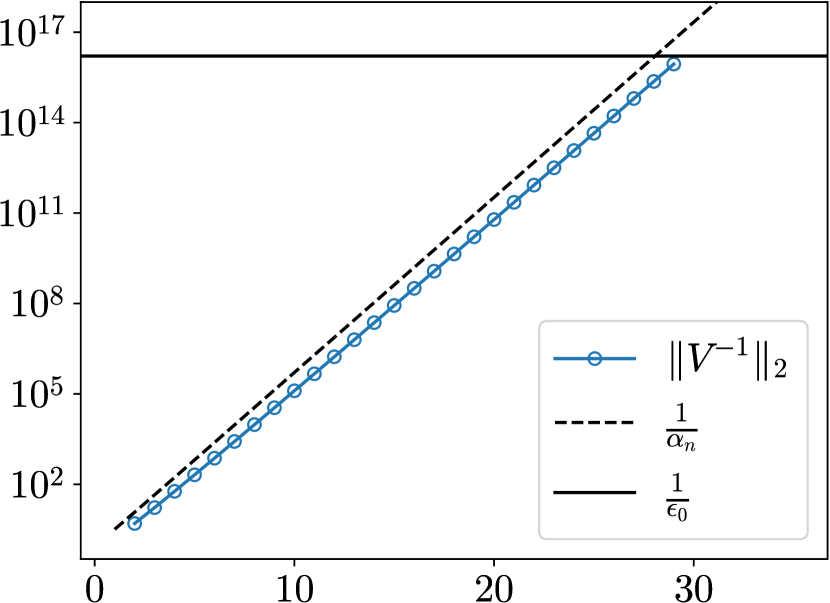
(a) $\gamma=10$: $a=1$, $b=10$

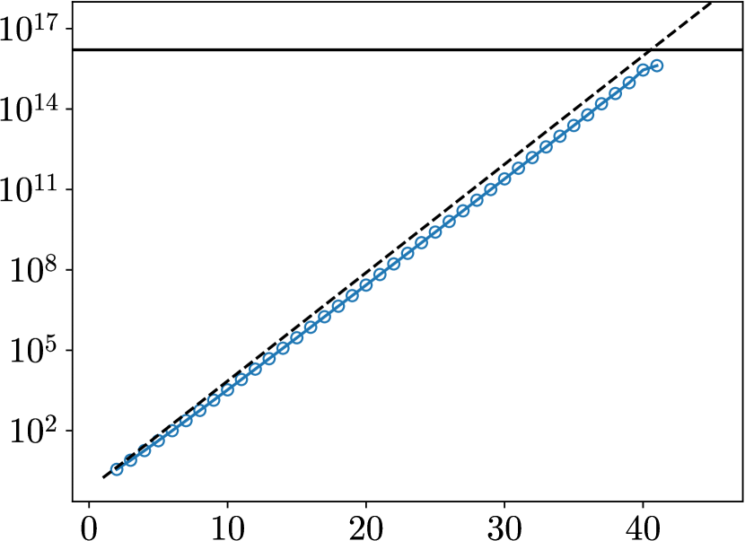
(b) $\gamma=50$: $a=1$, $b=50$

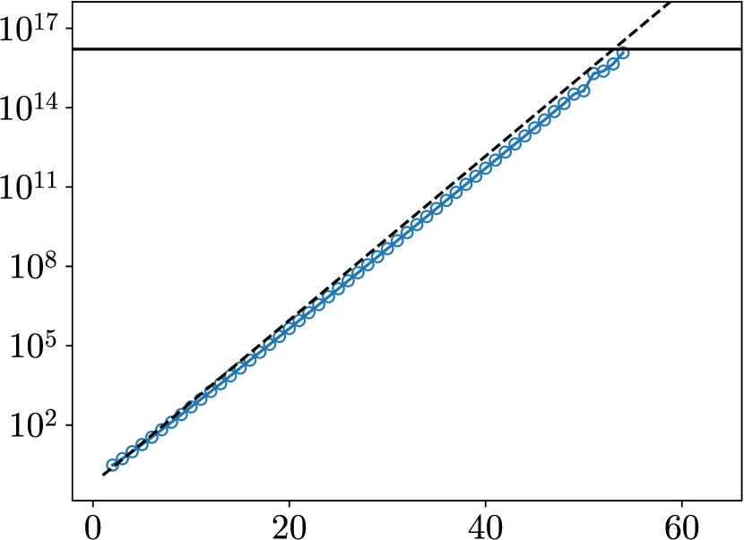
(c) $\gamma=250$: $a=1$, $b=250$

Figure 7: A comparison between ${\lVert V^{-1}\rVert}_{2}$ and $\frac{1}{\alpha_{n}}$, as a function of $n$, for $\gamma=10$, $50$, $250$.

10 Numerical Experiments

In this section, we demonstrate the performance of our algorithm with several numerical experiments. Our algorithm was implemented in Fortran 77, and compiled using the GFortran Compiler, version 12.2.0, with -O3 flag. All experiments were conducted on a laptop with 32 GB of RAM and an Intel $12$nd Gen Core i7-1270P CPU. A demo of our approximation scheme is provided in https://doi.org/10.5281/zenodo.8323315.

10.1 Approximation Over Varying Values of $n$

In this subsection, we approximate functions of the form $f(x)=\int_{a}^{b}x^{\mu}\sigma(\mu)\,d\mu$, $x\in[0,1]$, for the following cases of $\sigma(\mu)$:

$$\sigma_{1}(\mu) =\frac{1}{\mu},$$ (159)

$$\sigma_{2}(\mu) =\sin(12\mu),$$ (160)

$$\sigma_{3}(\mu) =e^{-10\mu},$$ (161)

$$\sigma_{4}(\mu) =\mu\sin(\mu).$$ (162)

We apply our algorithm with $N=n$ and $\epsilon=\epsilon_{0}$, where $\epsilon$ is the truncation point of the TSVD, as described in Theorem 7.3. We estimate $\|f-\widehat{f}_{N}\|_{L^{\infty}[0,1]}$, by evaluating $f$ and $\widehat{f}_{N}$ at $2000$ uniformly distributed points over $[0,1]$, and finding the maximum error between $f$ and $\widehat{f}_{N}$ at those points. We repeat the experiments for $\gamma=10$, $50$, $250$, and plot ${\|f-\widehat{f}_{N}\|_{L^{\infty}[0,1]}}/{|\sigma|}$. The results are displayed in Figures 8, 9 and 10.

It is evident that ${\|f-\widehat{f}_{N}\|_{L^{\infty}[0,1]}}/{|\sigma|}$ remains bounded by $\alpha_{n}$, as shown in Section 9, until it reaches a stabilized level that is close to machine precision multiplied by some small constant. Since $\{\alpha_{i}\}_{i=0,1,\ldots,\infty}$ decays exponentially, the approximation exhibits an exponential rate of convergence in $N$.

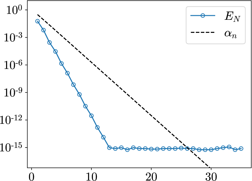
(a) $f(x)=\int_{1}^{10}x^{\mu}\sigma_{1}(\mu)\,d\mu$

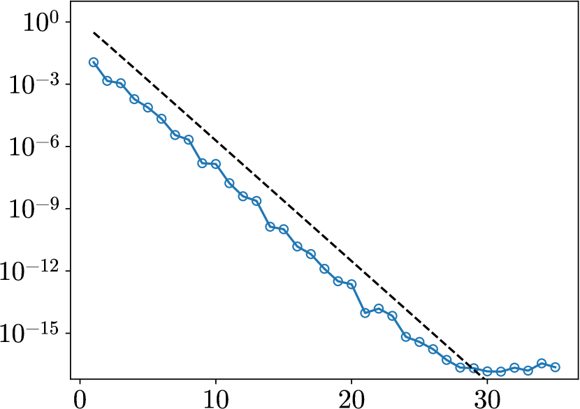
(b) $f(x)=\int_{1}^{10}x^{\mu}\sigma_{2}(\mu)\,d\mu$

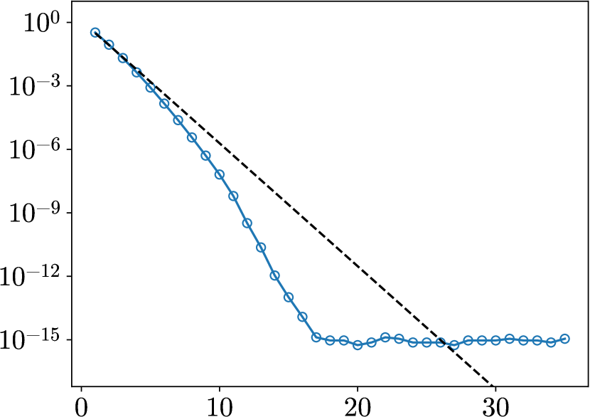
(c) $f(x)=\int_{1}^{10}x^{\mu}\sigma_{3}(\mu)\,d\mu$

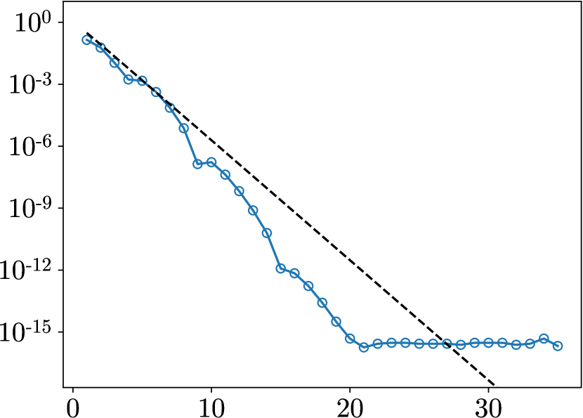
(d) $f(x)=\int_{1}^{10}x^{\mu}\sigma_{4}(\mu)\,d\mu$

Figure 8: The $L^{\infty}$ approximation error over $[0,1]$, $E_{N}:=\frac{\|f-\widehat{f}_{N}\|_{L^{\infty}[0,1]}}{|\sigma|}$, as a function of $n$, for $\gamma=10$.

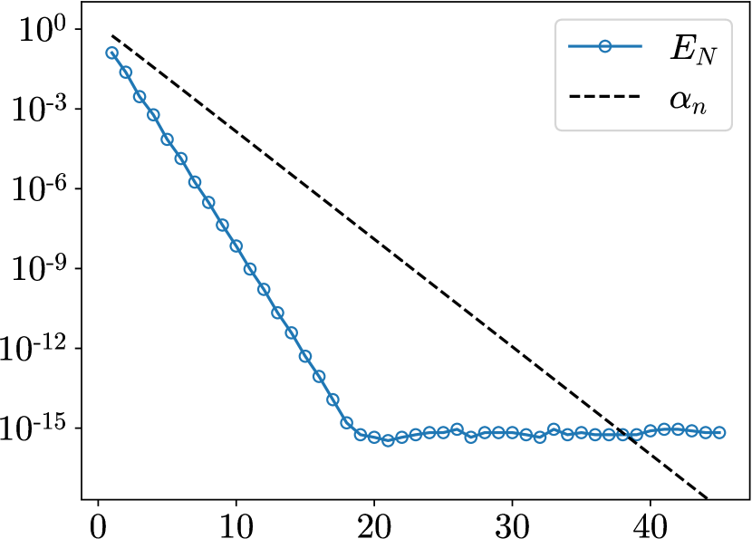
(a) $f(x)=\int_{1}^{50}x^{\mu}\sigma_{1}(\mu)\,d\mu$

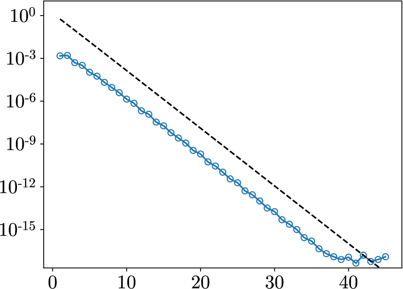
(b) $f(x)=\int_{1}^{50}x^{\mu}\sigma_{2}(\mu)\,d\mu$

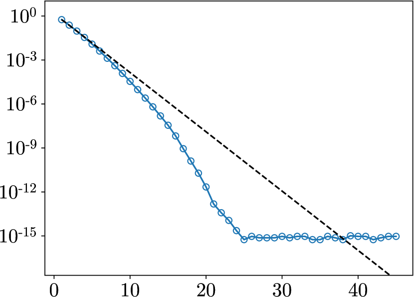
(c) $f(x)=\int_{1}^{50}x^{\mu}\sigma_{3}(\mu)\,d\mu$

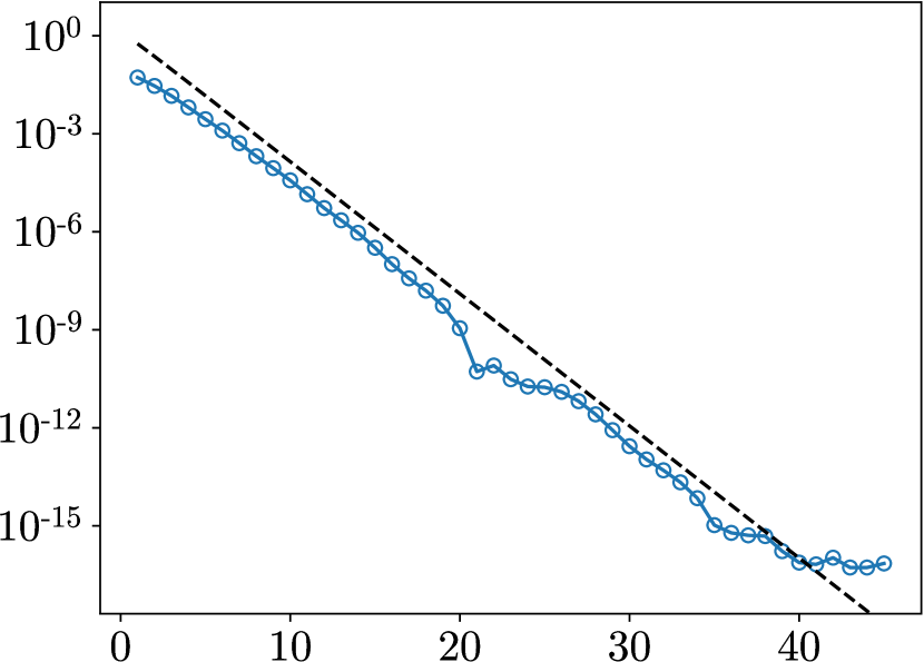
(d) $f(x)=\int_{1}^{50}x^{\mu}\sigma_{4}(\mu)\,d\mu$

Figure 9: The $L^{\infty}$ approximation error over $[0,1]$, $E_{N}:=\frac{\|f-\widehat{f}_{N}\|_{L^{\infty}[0,1]}}{|\sigma|}$, as a function of $n$, for $\gamma=50$.

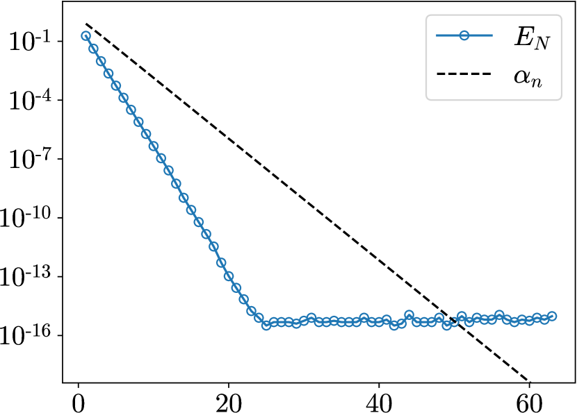
(a) $f(x)=\int_{1}^{250}x^{\mu}\sigma_{1}(\mu)\,d\mu$

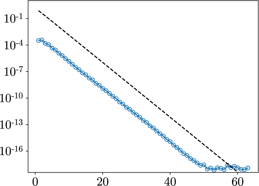
(b) $f(x)=\int_{1}^{250}x^{\mu}\sigma_{2}(\mu)\,d\mu$

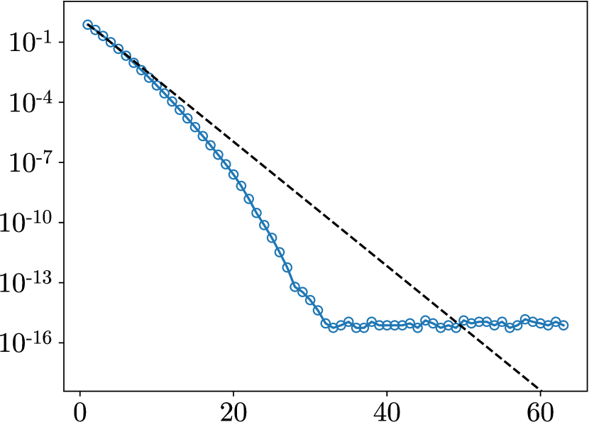
(c) $f(x)=\int_{1}^{250}x^{\mu}\sigma_{3}(\mu)\,d\mu$

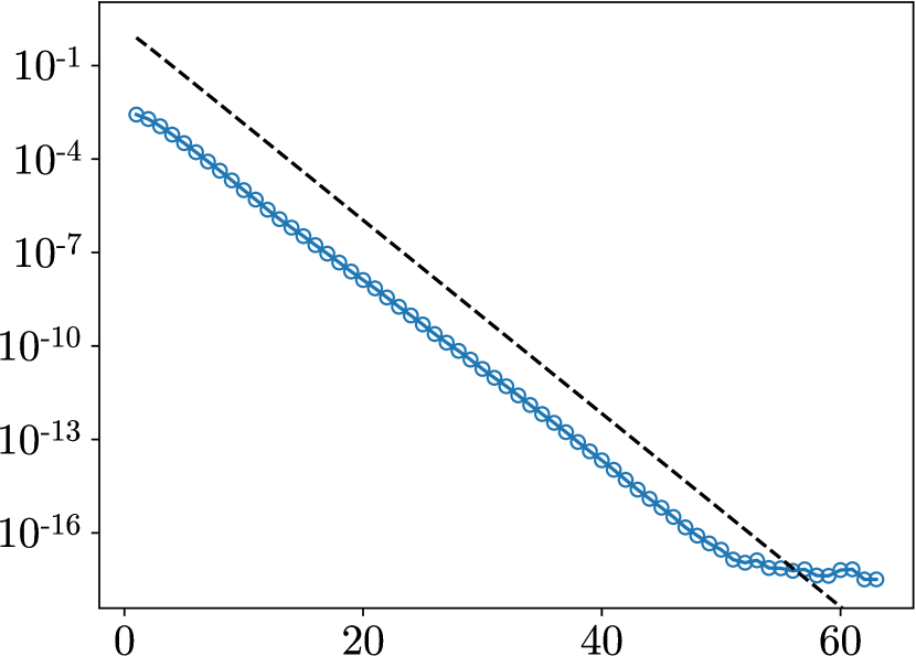
(d) $f(x)=\int_{1}^{250}x^{\mu}\sigma_{4}(\mu)\,d\mu$

Figure 10: The $L^{\infty}$ approximation error over $[0,1]$, $E_{N}:=\frac{\|f-\widehat{f}_{N}\|_{L^{\infty}[0,1]}}{|\sigma|}$, as a function of $n$, for $\gamma=250$.

10.2 Approximation of Non-integer Powers

In this subsection, our goal is to approximate functions of the form $f(x)=\int_{a}^{b}x^{\mu}\sigma(\mu)\,d\mu$, $x\in[0,1]$, with

$$\sigma_{5}(\mu)=\delta(\mu-c),$$ (163)

where $c\in[a,b]$. The resulting function is $f(x)=x^{c}$.

We fix $N=n$, where $\alpha_{n}\approx\epsilon_{0}$, and approximate such functions for $1000$ values of $c$ distributed logarithmically in the interval $[\frac{a}{1.5},1.5b]$. We set $\epsilon=\epsilon_{0}$, and evaluate $f$ and $\widehat{f}_{N}$ at $1000$ uniformly distributed points over $[0,1]$ to estimate ${\|f-\widehat{f}_{N}\|_{L^{\infty}[0,1]}}/{{\lvert\sigma\rvert}}$. The results for $\gamma=10,50,250$ are displayed in Figure 11. It can be observed that the approximation error remains accurate up to machine precision multiplied by some small constants, for values of $c$ within the interval $[a,b]$, and grows significantly, for values of $c$ outside $[a,b]$.

We further investigate the approximation error over varying values of $n$, for $c=a$, $\frac{a+b}{2}$, $b$ and $\gamma=10$, $50$, $250$, as shown in Figure 12. The approximation error is bounded by $\alpha_{n}$ multiplied by some small constants, until it stabilizes at a level around machine precision.

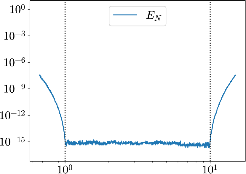
(a) $n=28$, $\gamma=10$: $a=1$, $b=10$

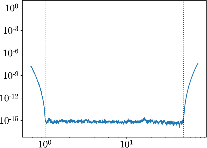
(b) $n=38$, $\gamma=50$: $a=1$, $b=50$

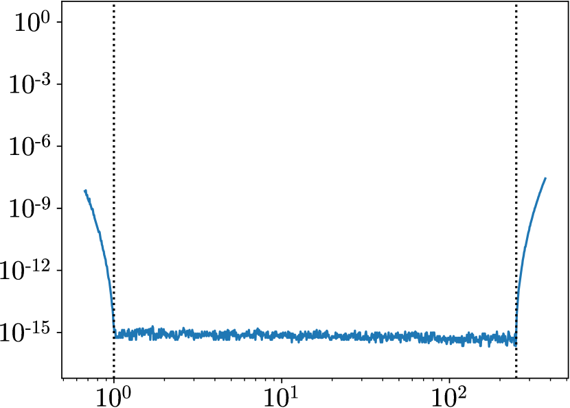
(c) $n=50$, $\gamma=250$: $a=1$, $b=250$

Figure 11: The $L^{\infty}$ approximation error of $f(x)=\int_{a}^{b}x^{\mu}\sigma_{5}(\mu)\,d\mu=x^{c}$ over $[0,1]$, $E_{N}:=\frac{\|f-\widehat{f}_{N}\|_{L^{\infty}[0,1]}}{|\sigma|}$, as a function of $c$, for a fixed $n$ such that $\alpha_{n}\approx\epsilon_{0}$, and for $\gamma=10$, $50$, $250$.

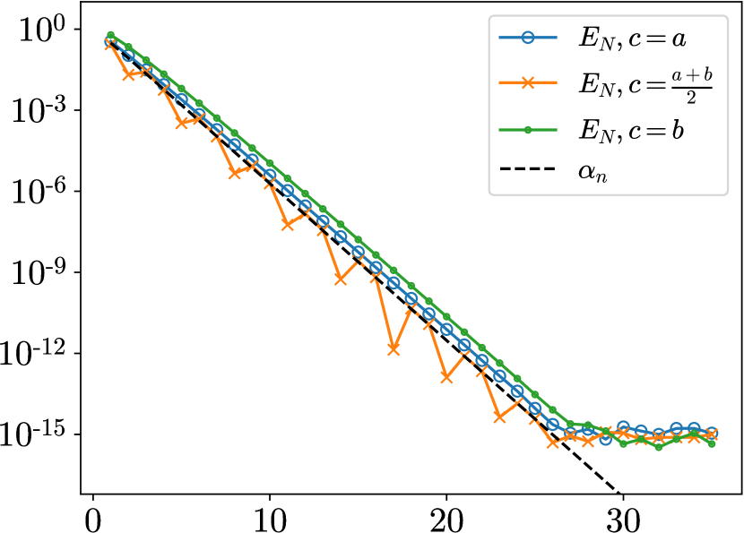
(a) $\gamma=10$: $a=1$, $b=10$

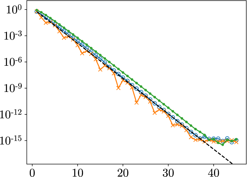
(b) $\gamma=50$: $a=1$, $b=50$

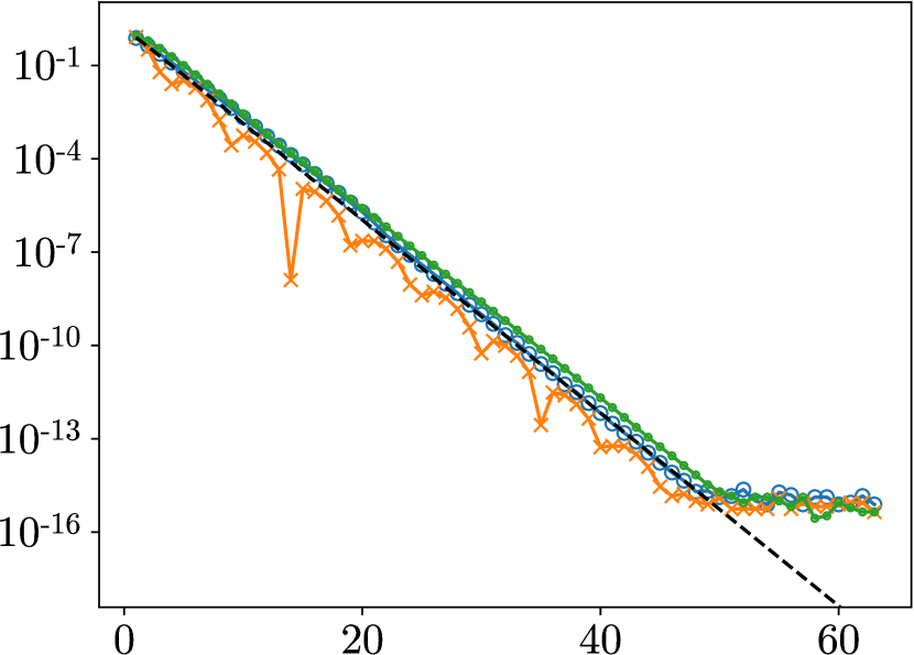
(c) $\gamma=250$: $a=1$, $b=250$

Figure 12: The $L^{\infty}$ approximation error of $f(x)=\int_{a}^{b}x^{\mu}\sigma_{5}(\mu)\,d\mu=x^{c}$ over $[0,1]$, $E_{N}:=\frac{\|f-\widehat{f}_{N}\|_{L^{\infty}[0,1]}}{|\sigma|}$, as a function of $n$, for $c=a$, $\frac{a+b}{2}$, $b$, and $\gamma=10$, $50$, $250$.

10.3 Approximation in the Case of Distributions

In this subsection, we assume $\sigma\in\mathcal{D}^{\prime}(\mathbbm{R})$ has the form

$$\sigma_{6}(\mu) =(-1)^{k}\delta^{(k)}(\mu-c),$$ (164)

where $k\geq 0$ is an integer, $c\in[a,b]$, and $\delta(t)$ is the Dirac delta function. The resulting function is $f(x)=x^{c}(\log{x})^{k}$. We apply our algorithm with $N=n$ and $\epsilon=\epsilon_{0}$, and evaluate $f$ and $\widehat{f}_{N}$ at $2000$ uniformly distributed points in $[0,1]$ to estimate ${\|f-\widehat{f}_{N}\|_{L^{\infty}[0,1]}}/{{\lvert\sigma\rvert}}$. The results for $k=1$, $2$, …, $6$, $c=a$, $\frac{a+b}{2}$, $b$, and $\gamma=10$, $50$, $250$ are shown in Figures 13, 14 and 15.

In contrast to the previous cases where $\sigma$ is a signed Radon measure, the approximation error can increase significantly with $k$. However, the approximation error is still bounded by $(\epsilon+\alpha_{n})\cdot\max_{0\leq i\leq n-1}{\bigl{\lVert}u_{i}\bigl{(}\tfrac{t-a}{b-a}\bigr{)}\bigr{\rVert}}_{C^{k}([a,b])}$, as stated in Theorem 8.1. Furthermore, we observe that the error grows with $k$, and when $c=a$, the error is closely aligned with the estimated bound, since the function is more singular for smaller $c$ and the approximation error tends to be larger.

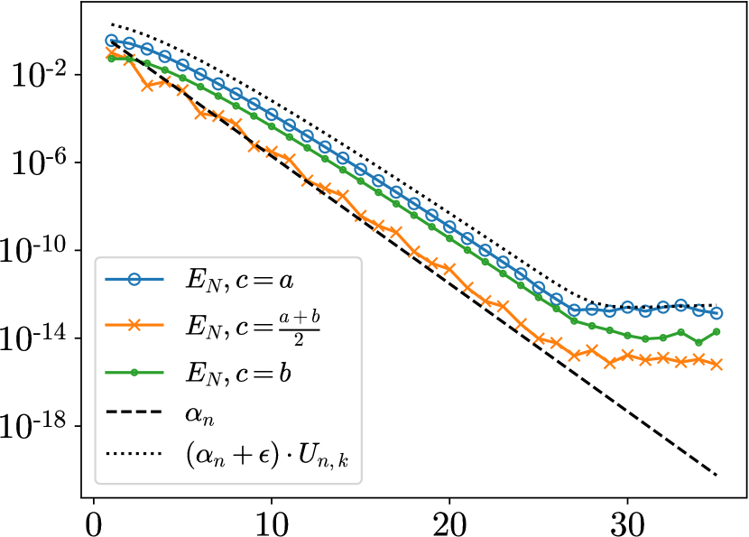
(a) $k=1$

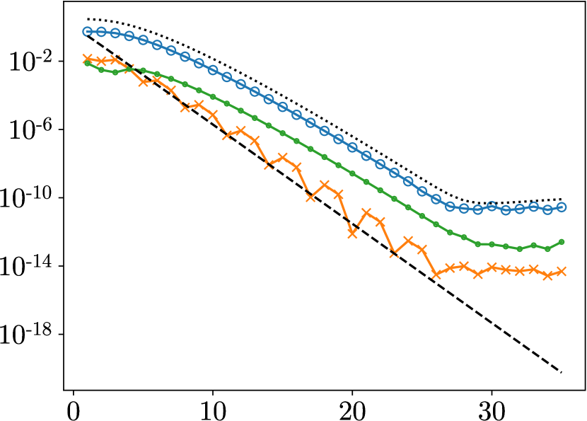
(b) $k=2$

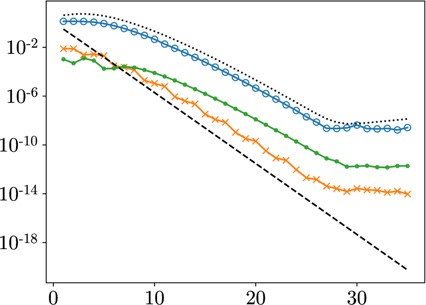
(c) $k=3$

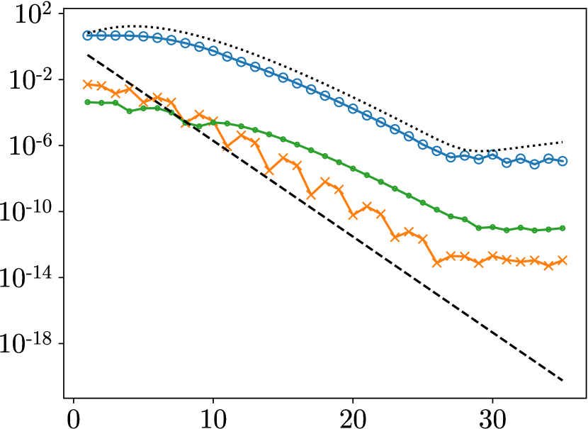
(d) $k=4$

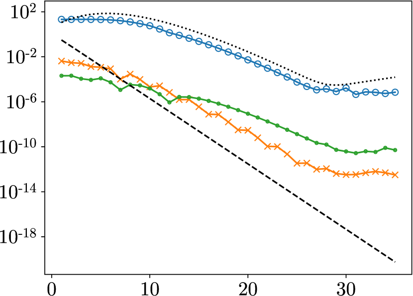
(e) $k=5$

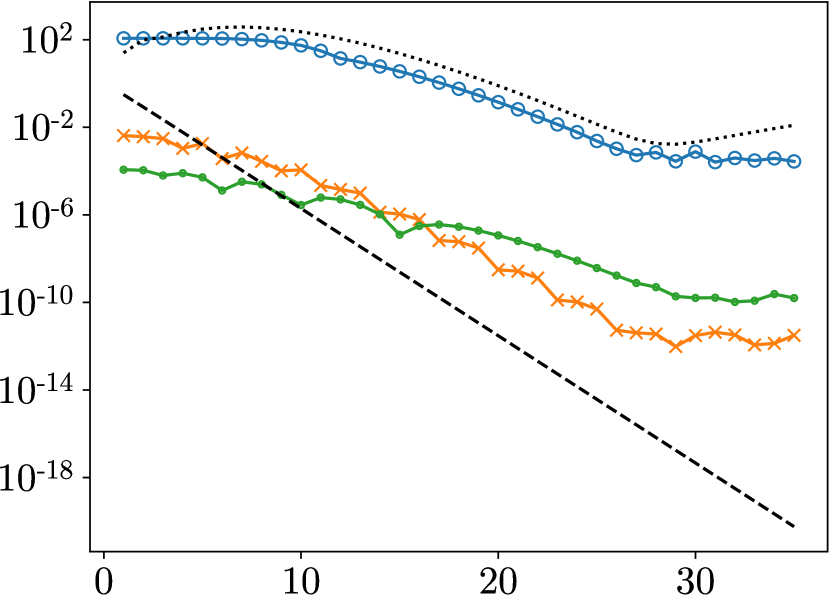
(f) $k=6$

Figure 13: The $L^{\infty}$ approximation error of $f(x)=\int_{1}^{10}x^{\mu}\sigma_{6}(\mu)\,d\mu=x^{c}(\log{x})^{k}$ over $[0,1]$, $E_{N}:=\frac{\|f-\widehat{f}_{N}\|_{L^{\infty}[0,1]}}{|\sigma|}$, as a function of $n$, for $c=a$, $\frac{a+b}{2}$, $b$, $k=1$, …, $6$, and $\gamma=10$. $U_{n,k}:=\max_{0\leq i\leq n-1}{\bigl{\lVert}u_{i}\bigl{(}\tfrac{t-a}{b-a}\bigr{)}\bigr{\rVert}}_{C^{k}([a,b])}$.

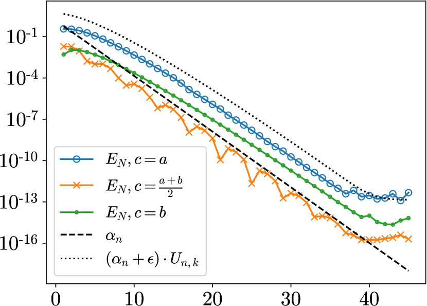
(a) $k=1$

(b) $k=2$

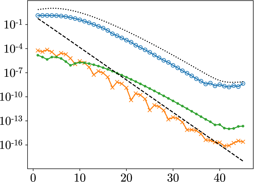
(c) $k=3$

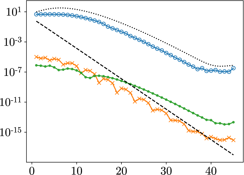
(d) $k=4$

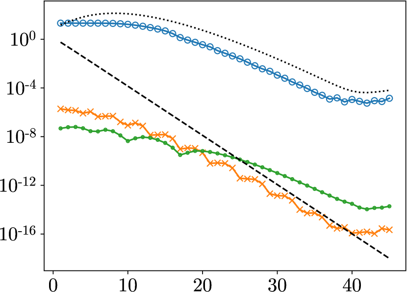
(e) $k=5$

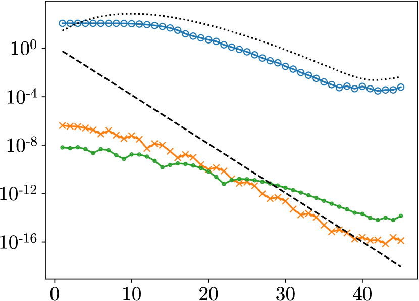
(f) $k=6$

Figure 14: The $L^{\infty}$ approximation error of $f(x)=\int_{1}^{50}x^{\mu}\sigma_{6}(\mu)\,d\mu=x^{c}(\log{x})^{k}$ over $[0,1]$, $E_{N}:=\frac{\|f-\widehat{f}_{N}\|_{L^{\infty}[0,1]}}{|\sigma|}$, as a function of $n$, for $c=a$, $\frac{a+b}{2}$, $b$, $k=1$, …, $6$, and $\gamma=50$. $U_{n,k}:=\max_{0\leq i\leq n-1}{\bigl{\lVert}u_{i}\bigl{(}\tfrac{t-a}{b-a}\bigr{)}\bigr{\rVert}}_{C^{k}([a,b])}$.

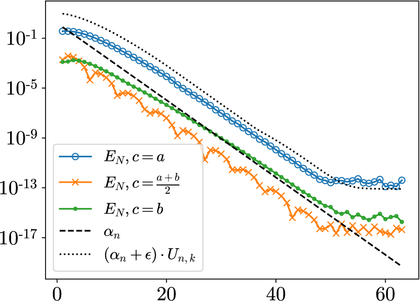
(a) $k=1$

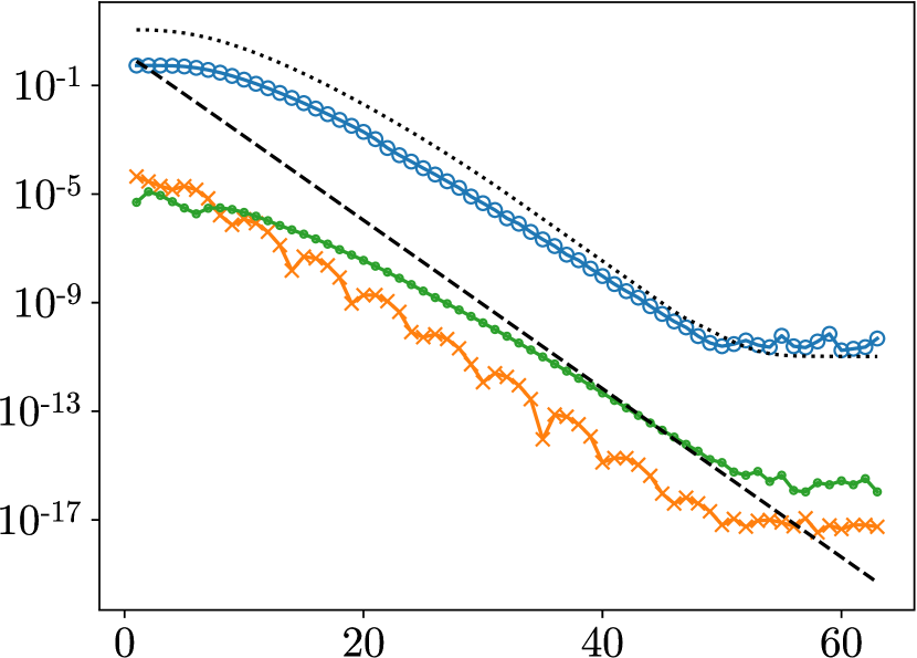
(b) $k=2$

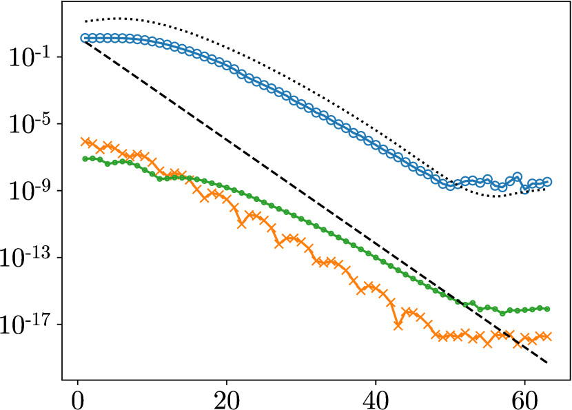
(c) $k=3$

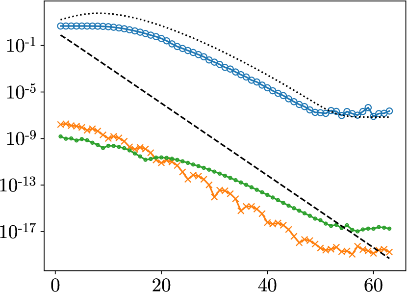
(d) $k=4$

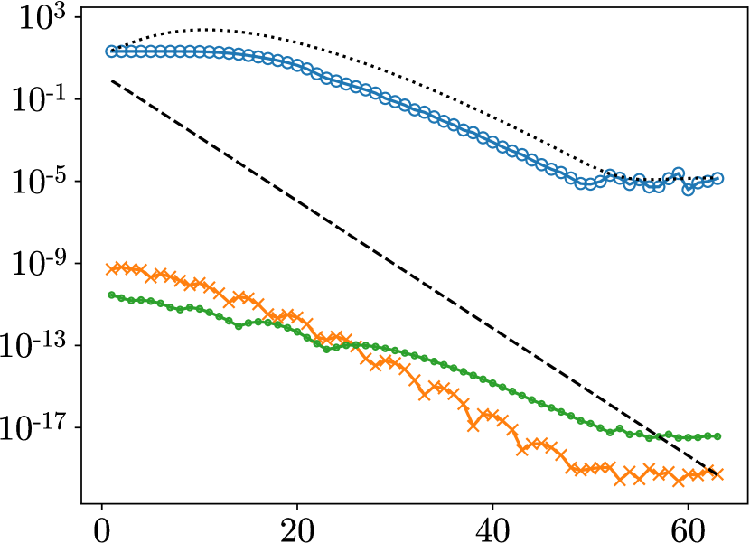
(e) $k=5$

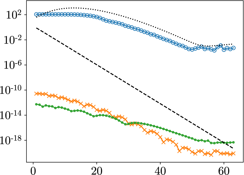
(f) $k=6$

Figure 15: The $L^{\infty}$ approximation error of $f(x)=\int_{1}^{250}x^{\mu}\sigma_{6}(\mu)\,d\mu=x^{c}(\log{x})^{k}$ over $[0,1]$, $E_{N}:=\frac{\|f-\widehat{f}_{N}\|_{L^{\infty}[0,1]}}{|\sigma|}$, as a function of $n$, for $c=a$, $\frac{a+b}{2}$, $b$, $k=1$, …, $6$, and $\gamma=250$. $U_{n,k}:=\max_{0\leq i\leq n-1}{\bigl{\lVert}u_{i}\bigl{(}\tfrac{t-a}{b-a}\bigr{)}\bigr{\rVert}}_{C^{k}([a,b])}$.

10.4 Approximation Over a Simple Arc in the Complex Plane

In this subsection, we investigate the performance of our algorithm on simple and smooth arcs in the complex plane. Suppose that $\widetilde{\gamma}\colon[0,1]\rightarrow\mathbb{C}$, and let $\Gamma=\widetilde{\gamma}([0,1])$. We replace the interpolation matrix V in Equation 105 by a modified interpolation matrix $V_{\Gamma}$, defined by

$$V_{\Gamma}=\begin{pmatrix}\widetilde{\gamma}(x_{1})^{t_{1}}&\widetilde{\gamma}(x_{1})^{t_{2}}&\ \ldots&\ \widetilde{\gamma}(x_{1})^{t_{N}}\\ \widetilde{\gamma}(x_{2})^{t_{1}}&\widetilde{\gamma}(x_{2})^{t_{2}}&\ \ldots&\ \widetilde{\gamma}(x_{2})^{t_{N}}\\ \vdots&\vdots&\ \ddots&\vdots\\ \widetilde{\gamma}(x_{N})^{t_{1}}&\widetilde{\gamma}(x_{N})^{t_{2}}&\ \ldots&\ \widetilde{\gamma}(x_{N})^{t_{N}}\end{pmatrix}\in\mathbb{C}^{N\times N}.$$ (165)

Specifically, we consider the arcs $\widetilde{\gamma}(t)=t+\alpha i(t^{2}-t)$, for $\alpha=0.8$, $1.6$ and $2.4$, which are plotted in Figure 16. Our goal is to approximate functions of the form

$$f_{\Gamma}(t):=\int_{a}^{b}\widetilde{\gamma}(t)^{\mu}\sigma(\mu)\,d\mu,$$ (166)

over the arcs $\widetilde{\gamma}(t)$, where $t\in[0,1]$. We apply the algorithm with $N=n$ and $\epsilon=\epsilon_{0}$ to the functions $f_{\Gamma}(t)$ where $\sigma(\mu)$ has the forms $\sigma_{3}(\mu)$ and $\sigma_{4}(\mu)$, as defined in Equation 161 and Equation 162, respectively. The experiments are repeated for $\gamma=10,50,250$, and the results are displayed in Figures 17, 18 and 19.

We also investigate the approximation errors for non-integer powers $f_{\Gamma}(t)=\widetilde{\gamma}(t)^{c}$ over the arcs $\widetilde{\gamma}(t)$, where $c\in[\frac{a}{1.5},1.5b]$, following the same procedure as the one described in Section 10.2. The results are displayed in Figure 20.

By analyzing the approximation errors over $\widetilde{\gamma}(t)$, for different values of $\alpha$, we observe that the approximation error grows with $\alpha$, and depends on the specific functions being approximated. Generally, when $\gamma$ is small, the approximation error grows only slightly as the arc becomes more curved, while for large $\gamma$, it is possible for the approximation error to grow significantly larger than $\alpha_{n}$. When the arc is slightly curved, the approximation performs similarly to the cases where $\widetilde{\gamma}(t)=[0,1]$, with the error bounded by $\alpha_{n}$.

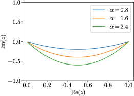
Figure 16: $\widetilde{\gamma}(t)=t+\alpha i(t^{2}-t)$.

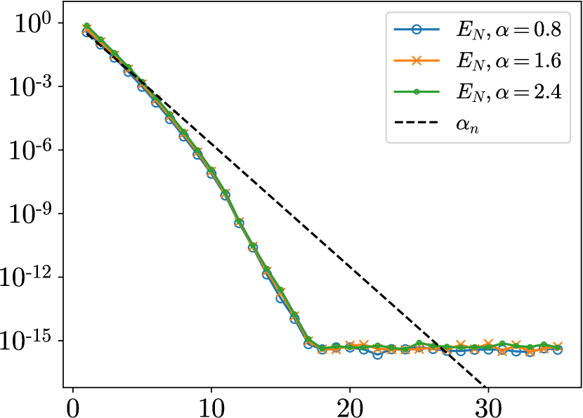
(a) $f_{\Gamma}(t)=\int_{1}^{10}\widetilde{\gamma}(t)^{\mu}\sigma_{3}(\mu)\,d\mu$

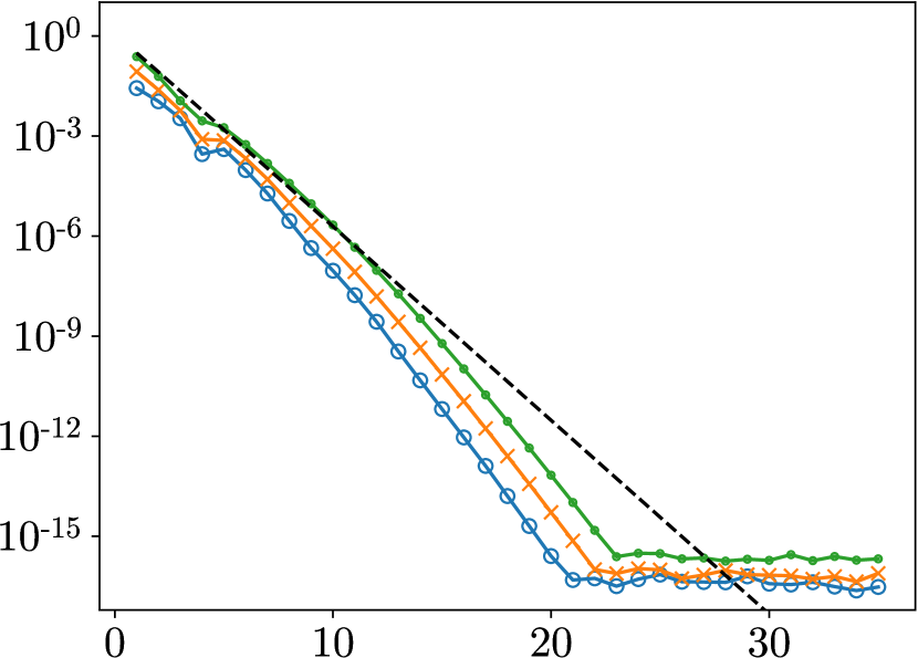
(b) $f_{\Gamma}(t)=\int_{1}^{10}\widetilde{\gamma}(t)^{\mu}\sigma_{4}(\mu)\,d\mu$

Figure 17: The $L^{\infty}$ approximation error over $\widetilde{\gamma}(t)$, $E_{N}:=\frac{\|f_{\Gamma}-\widehat{f}_{N}\|_{L^{\infty}[0,1]}}{|\sigma|}$, as a function of $n$, for $\alpha=0.8$, $1.6$, $2.4$, and $\gamma=10$.

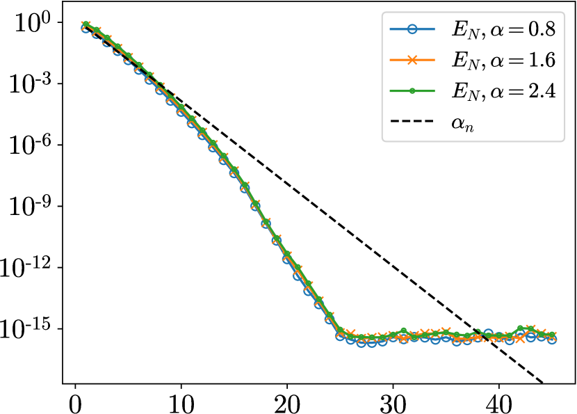
(a) $f_{\Gamma}(t)=\int_{1}^{50}\widetilde{\gamma}(t)^{\mu}\sigma_{3}(\mu)\,d\mu$

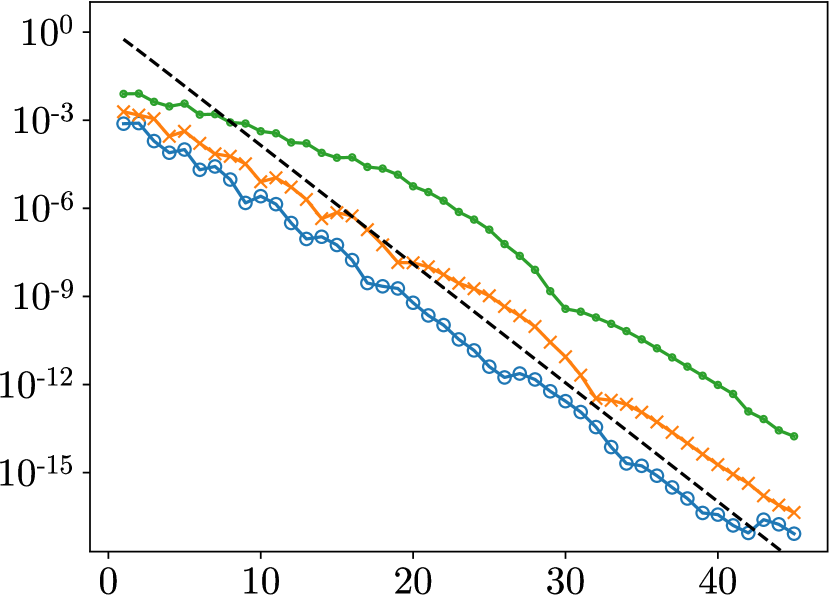
(b) $f_{\Gamma}(t)=\int_{1}^{50}\widetilde{\gamma}(t)^{\mu}\sigma_{4}(\mu)\,d\mu$

Figure 18: The $L^{\infty}$ approximation error over $\widetilde{\gamma}(t)$, $E_{N}:=\frac{\|f_{\Gamma}-\widehat{f}_{N}\|_{L^{\infty}[0,1]}}{|\sigma|}$, as a function of $n$, for $\alpha=0.8$, $1.6$, $2.4$, and $\gamma=50$.

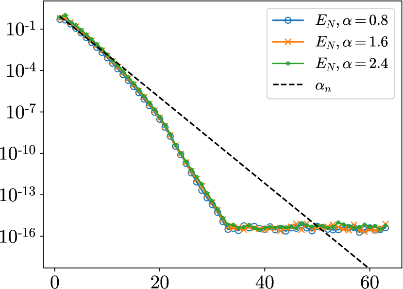
(a) $f_{\Gamma}(t)=\int_{1}^{250}\widetilde{\gamma}(t)^{\mu}\sigma_{3}(\mu)\,d\mu$

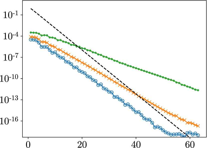
(b) $f_{\Gamma}(t)=\int_{1}^{250}\widetilde{\gamma}(t)^{\mu}\sigma_{4}(\mu)\,d\mu$

Figure 19: The $L^{\infty}$ approximation error over $\widetilde{\gamma}(t)$, $E_{N}:=\frac{\|f_{\Gamma}-\widehat{f}_{N}\|_{L^{\infty}[0,1]}}{|\sigma|}$, as a function of $n$, for $\alpha=0.8$, $1.6$, $2.4$, and $\gamma=250$.

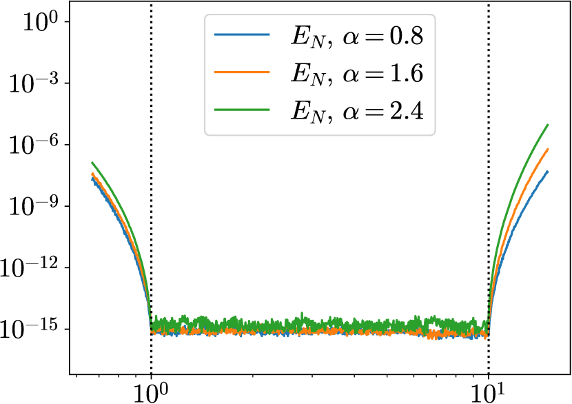
(a) $n=32$, $\gamma=10$: $a=1$, $b=10$

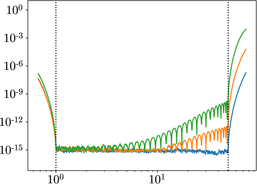
(b) $n=42$, $\gamma=50$: $a=1$, $b=50$

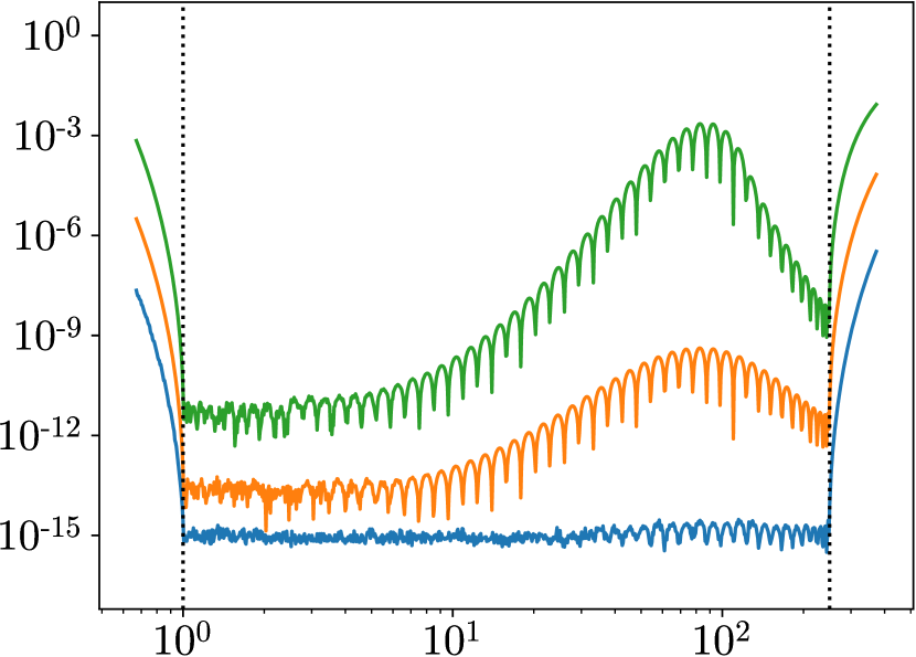
(c) $n=55$, $\gamma=250$: $a=1$, $b=250$

Figure 20: The $L^{\infty}$ approximation error of $f_{\Gamma}(t)=\int_{a}^{b}\widetilde{\gamma}(t)^{\mu}\sigma_{5}(\mu)\,d\mu=\widetilde{\gamma}(t)^{c}$ over $\widetilde{\gamma}(t)$, $E_{N}:=\frac{\|f_{\Gamma}-\widehat{f}_{N}\|_{L^{\infty}[0,1]}}{|\sigma|}$, as a function of $c$, for a fixed $n$ such that $\alpha_{n}\approx\epsilon_{0}$, $\alpha=0.8$, $1.6$, $2.4$, and $\gamma=10$, $50$, $250$.

10.5 Tapered Exponential Clustering of the Collocation Points

We observe that the collection of collocation points $\{x_{j}\}_{j=1}^{N}$ generated by our algorithm exhibits a tapered exponential clustering around the singularity at $x=0$. Specifically, the density of $\{x_{j}\}_{j=1}^{N}$ over $[0,1]$ tapers in the direction of $x=0$, when viewed on a logarithmic scale. This observation is demonstrated in Figure 21, for $\gamma=10$, $50$, $250$, and for $n$ ranging from $1$ to the value of $n$ where $\alpha_{n}\approx\epsilon_{0}$.

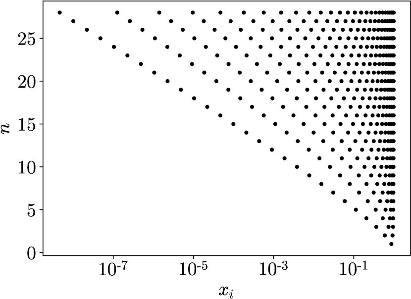
(a) $\gamma=10$: $a=1$, $b=10$

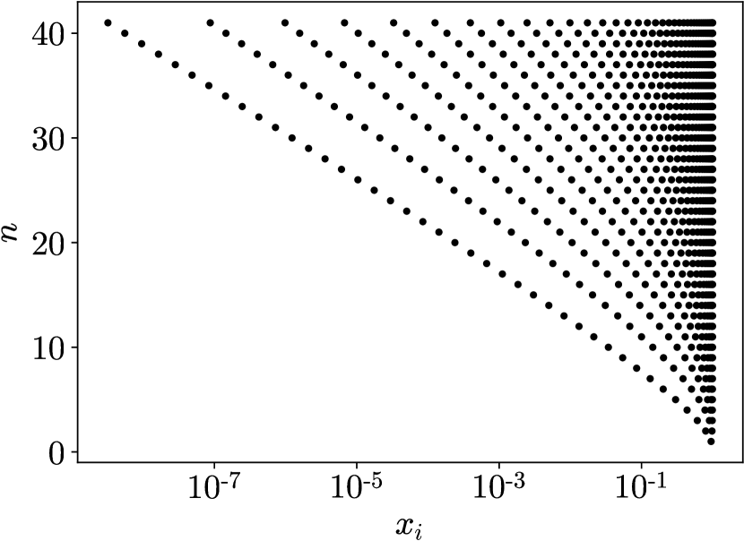
(b) $\gamma=50$: $a=1$, $b=50$

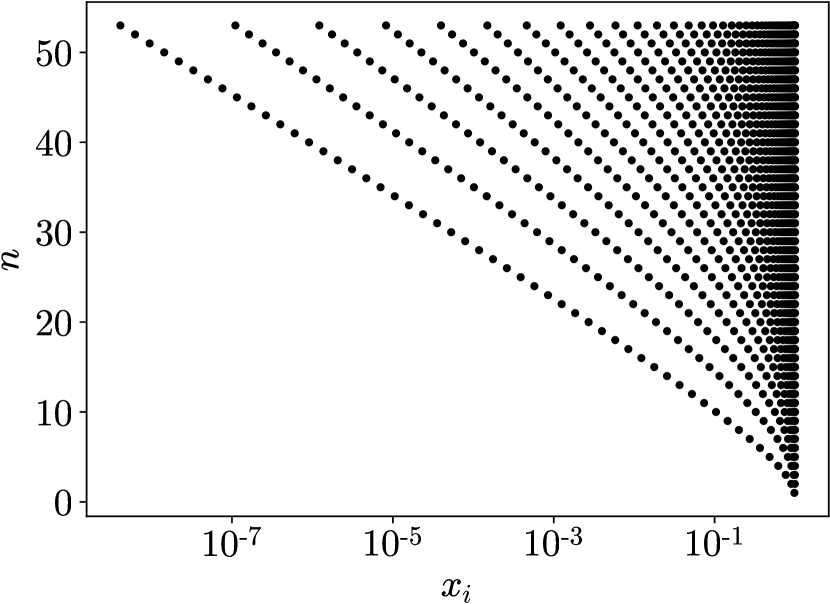
(c) $\gamma=250$: $a=1$, $b=250$

Figure 21: The distribution of collocation points $\{x_{j}\}_{j=1}^{N}$ over $[0,1]$, for values of $n$ such that $\alpha_{n}\gtrsim\epsilon_{0}$, and $\gamma=10$, $50$, $250$.

11 Conclusion

In this paper, we introduce an approach to approximate functions of the form $f(x)=\int_{a}^{b}x^{\mu}\sigma(\mu)\,d\mu$ over the interval $[0,1]$, by expansions in a small number of singular powers $x^{t_{1}}$, $x^{t_{2}}$, …, $x^{t_{N}}$, where $0<a<b<\infty$ and $\sigma(\mu)$ is some signed Radon measure or some distribution supported on $[a,b]$. Given any desired accuracy $\epsilon$, our method guarantees that the uniform approximation error over the entire interval $[0,1]$ is bounded by $\epsilon$ multiplied by certain small constants. Additionally, the number of basis functions $N$ grows asymptotically as $O(\log{\frac{1}{\epsilon}})$, and the expansion coefficients can be found by collocating the function at specially chosen collocation points $x_{1}$, $x_{2}$, …, $x_{N}$ and solving an $N\times N$ linear system numerically. In practice, when $\frac{b}{a}=10$ and $\sigma$ is a signed Radon measure, our method requires only approximately $N=30$ basis functions and collocation points in order to achieve machine precision accuracy. Numerical experiments demonstrate that our method can also be used for approximation over simple smooth arcs in the complex plane. A key feature of our method is that both the basis functions and the collocation points are determined a priori by only the values of $a$, $b$, and $\epsilon$. This sets it apart from expert-driven approximation methods, and from other methods that rely on careful selection of parameters to determine the basis functions. For example, the basis functions used in rational and reciprocal-log approximation are defined by the locations of poles, and the SE-Sinc and DE-Sinc approximations depend on the choices of smooth transformations. Compared to the DE-Sinc approximation, which achieves nearly-exponential rates of convergence at the cost of doubly-exponentially clustered collocation points, our method uses collocation points which exhibit only tapered exponential clustering. Compared to reciprocal-log approximation, which requires the least-squares solution of an overdetermined linear system with many collocation points, our method involves the solution of a small square linear system to determine the expansion coefficients.

Since our method approximates singular functions accurately by expansions in singular powers, it can be used with existing finite element methods or integral equation methods to approximate the solutions of PDEs on nonsmooth geometries or with discontinuous data. Typically, the leading singular terms of the asymptotic expansions of solutions near corners are derived from the angles at the corners, and are added to the basis functions of finite element methods to enhance the convergence rates (see, for example, [33], [8], [26]). Now, with only the knowledge that the singular solutions are of the form Equation 78, we can enhance the convergence rates of finite element methods without knowledge of the angles at the corners, by adding all of the singular powers obtained from our method to the basis functions. Likewise, the singular powers obtained from our method can be used in integral equation methods for PDEs. In integral equation methods, boundary value problems for PDEs are reformulated as integral equations for boundary charge and dipole densities which represent their solutions. Previously, singular asymptotic expansions of the densities, determined by the angles at the corners, were used to construct special quadrature rules to solve these integral equations (see, for example, [28], [29]). Using only the fact that the singular densities are of the form Equation 78, quadrature rules can instead be developed for only the singular powers obtained from our method, independent of the angles at the corners.

References

- [1] Babuška, I., B. Andersson, B. Guo, J. M. Melenk, and H. S. Oh. “Finite element method for solving problems with singular solutions.” J. Comput. Appl. Math. 74 (1996): 51–70.
- [2] Bauer, F.L., and C.T. Fike. “Norms and exclusion theorems.” Numer. Math. 2.1 (1960): 137–141.
- [3] Bertero, M., P. Boccacci, and E.R. Pike. “On the recovery and resolution of exponential relaxation rates from experimental data: a singular-value analysis of the Laplace transform inversion in the presence of noise.” P. Roy. Soc. A-Math. Phy. 383 (1982): 15–29.
- [4] Beylkin, G., and L. Monzón. “On approximation of functions by exponential sums.” Appl. Comput. Harmon. A. 19.1 (2005): 1063–5203.
- [5] Chen, S., and J. Shen. “Enriched spectral methods and applications to problems with weakly singular solutions.” J. Sci. Comput. 77 (2018): 1468–1489.
- [6] Coppé, V., D. Huybrechs, R. Matthysen, and M. Webb. “The AZ algorithm for least squares systems with a known incomplete generalized inverse.” SIAM J. Matrix Anal. A. 41.3 (2020): 1237–1259.
- [7] Filip, S., Y. Nakatsukasa, L. N. Trefethen, and B. Beckermann. “Rational minimax approximation via adaptive barycentric representations.” SIAM J. Sci. Comput. 40.4 (2018): A2427–A2455.
- [8] Fix, G. J., S. Gulati, and G. I. Wakoff. “On the use of singular functions with finite element approximations.” J. Comput. Phys. 13.2 (1973): 209–228.
- [9] Fries, T.-P., and T. Belytschko. “The extended/generalized finite element method: an overview of the method and its applications.” Int. J. Numer. Methods Eng. 84.3 (2010): 253–304.
- [10] Gončar, A. A. “On the rapidity of rational approximation of continuous functions with characteristic singularities.” Math. USSR-Sb. 2.4 (1967): 561–568.
- [11] Gopal, A., and L. N. Trefethen. “New Laplace and Helmholtz solvers.” Proc. Natl. Acad. Sci. 116.21 (2019): 10223–10225.
- [12] Gopal, A., and L. N. Trefethen. “Solving Laplace Problems with corner singularities via rational functions.” SIAM J. Numer. Anal. 57.5 (2019): 2074–2094.
- [13] Gutknecht, M. H., and L. N. Trefethen. “Nonuniqueness of best rational Chebyshev approximations on the unit disk.” J. Approx. Theory 39.3 (1983): 275–288.
- [14] Hansen, P.C. “The truncated SVD as a method for regularization.” BIT. 27.4 (1987): 534–553.
- [15] Herremans, A., and D. Huybrechs. “Efficient function approximation in enriched approximation spaces.” ArXiv 2023.
- [16] Lederman, R.R., and V. Rokhlin. “On the analytical and numerical properties of the truncated Laplace transform I.” SIAM J. Numer. Anal. 53.3 (2015): 1214–1235.
- [17] Lederman, R.R., and V. Rokhlin. “On the analytical and numerical properties of the truncated Laplace transform. Part II.” SIAM J. Numer. Anal. 54.2 (2016): 665–687.
- [18] Lehman, R. S. “Developments at an Analytic Corner of Solutions of Elliptic Partial Differential Equations.” J. Math. Mech. 8.5 (1959): 727–760.
- [19] Lucas, T. R., and H. S. Oh. “The method of auxiliary mapping for the finite element solutions of elliptic problems containing singularities.” J. Comput. Phys. 108.2 (1993): 327–342.
- [20] Mori, M. “ Discovery of the Double Exponential Transformation and Its Developments.” Publ. Res. Inst. Math. Sci. 41 (2005): 897–935.
- [21] Nakatsukasa, Y., and L. N. Trefethen. “An algorithm for real and complex rational minimax approximation.” SIAM J. Sci. Comput. 42.5 (2020): A3157–A3179.
- [22] Nakatsukasa, Y., and L. N. Trefethen. “Reciprocal-log approximation and planar PDE solvers.” SIAM J. Numer. Anal. 59.6 (2021): 2801–2822.
- [23] Nakatsukasa, Y., O. Sète, and L. N. Trefethen. “The AAA algorithm for rational approximation.” SIAM J. Sci. Comput. 40.3 (2018): A1494–A1522.
- [24] Newman, D. J. “Rational approximation to .” Mich. Math. J. 11.1 (1964): 11–14.
- [25] Okayama, T., T. Matsuo, and M. Sugihara. “Sinc-collocation methods for weakly singular Fredholm integral equations of the second kind.” J. Comput. Appl. Math. 234.4 (2010): 1211–1227.
- [26] Olson, L. G., G. C. Georgiou, and W. W. Schultz. “An efficient finite element method for treating singularities in Laplace’s Equation.” J. Comput. Phys. 96.2 (1991): 391–410.
- [27] Roache, P. J. “A pseudo-spectral FFT technique for non-periodic problems.” J. Comput. Phys. 27.2 (1978): 204–220.
- [28] Serkh, K. “On the Solution of Elliptic Partial Differential Equations on Regions with Corners.” J. Comput. Phys. 305 (2016): 150–171.
- [29] Serkh, K., and V. Rokhlin. “On the solution of the Helmholtz equation on regions with corners.” Proc. Natl. Acad. Sci. 113.33 (2016): 9171–9176.
- [30] Stahl, H. “Best uniform rational approximation of on .” Acta. Math. 190 (2003): 241–306.
- [31] Stenger, F. “Explicit nearly optimal linear rational approximation with preassigned poles.” Math. Comput. 47.175 (1986): 225–252.
- [32] Stenger, F. “Numerical Methods Based on Sinc and Analytic Functions in numerical Analysis.” SSCM Springer-Verlag, 1993.
- [33] Tong, P., and T. H. H. Pian. “On the convergence of the finite element method for problems with singularity.” Int. J. Solids Struct. 9.3 (1973): 313–321.
- [34] Trefethen, L. N., Y. Nakatsukasa, and J. A. C. Weideman. “Exponential node clustering at singularities for rational approximation, quadrature, and PDEs.” Numer. Math. 147.1 (2021): 227–254.
- [35] Wasow, W. “Asymptotic development of the solution of Dirichlet’s problem at analytic corners.” Duke Math. J. 24.1 (1957): 47–56.