STAEformer: Spatio-Temporal Adaptive Embedding Makes Vanilla Transformer SOTA for Traffic Forecasting

Abstract.

With the rapid development of the Intelligent Transportation System (ITS), accurate traffic forecasting has emerged as a critical challenge. The key bottleneck lies in capturing the intricate spatio-temporal traffic patterns. In recent years, numerous neural networks with complicated architectures have been proposed to address this issue. However, the advancements in network architectures have encountered diminishing performance gains. In this study, we present a novel component called spatio-temporal adaptive embedding that can yield outstanding results with vanilla transformers. Our proposed Spatio-Temporal Adaptive Embedding transformer (STAEformer) achieves state-of-the-art performance on six real-world traffic forecasting datasets. Further experiments demonstrate that spatio-temporal adaptive embedding plays a crucial role in traffic forecasting by effectively capturing intrinsic spatio-temporal relations and chronological information in traffic time series.

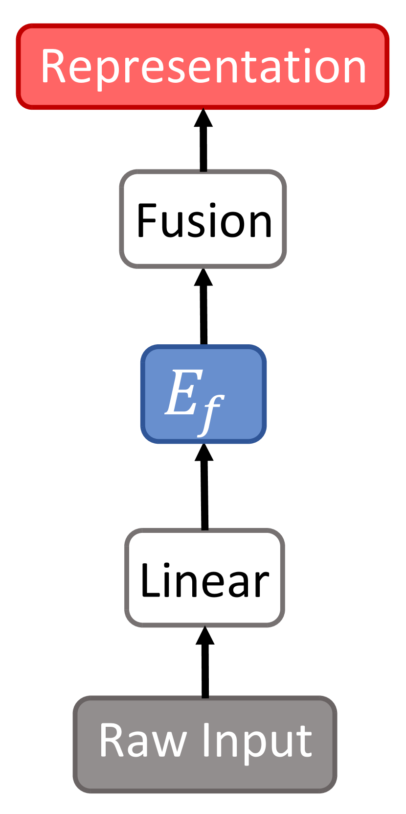
(a) STGNNs

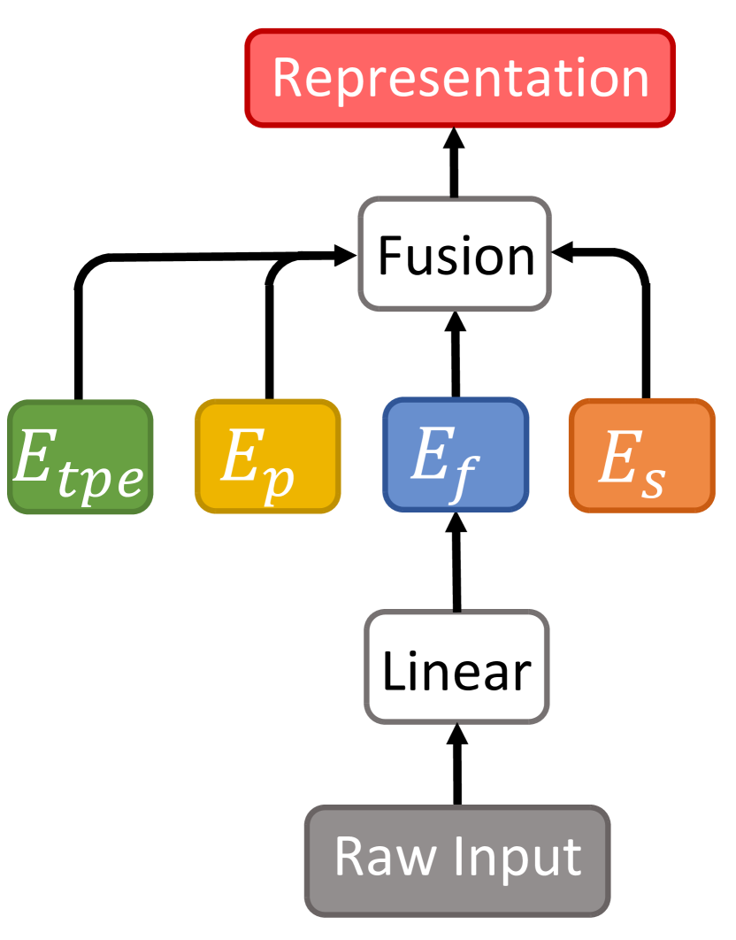
(b) Transformer-
based Models

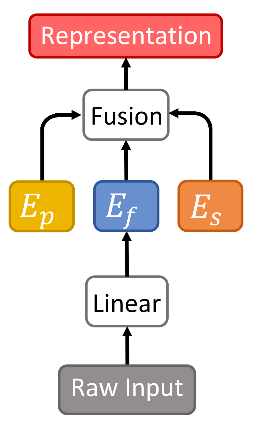
(c) Spatial Temporal Identity

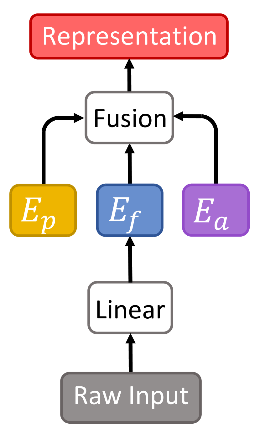
(d) Ours

Figure 1. Input Embeddings in Different Traffic Models.

1. Introduction

Traffic forecasting (Jiang et al., 2021) aims to predict the future traffic time series in road networks based on historical observations. In recent years, the success of deep learning models has been notable, primarily attributable to their ability to capture the inherent spatio-temporal dependencies in the traffic system. Among them, Spatio-Temporal Graph Neural Networks (STGNNs) (Yu et al., 2018; Li et al., 2018) and Transformer-based models (Guo et al., 2019; Zheng et al., 2020; Xu et al., 2020; Jiang et al., 2023a) become very popular for their outstanding performance. Researchers have devoted considerable effort to developing fancy and complicated models for traffic forecasting, such as novel graph convolutions (Cao et al., 2020; Song et al., 2020; Li and Zhu, 2021; Diao et al., 2019; Ye et al., 2021; Han et al., 2021; Wang et al., 2020; Zhao et al., 2019; Chen et al., 2021; Guo et al., 2021; Wang et al., 2022; Fang et al., 2021; Lu et al., 2020), learning graph structures (Wu et al., 2019; Jiang et al., 2023b; Shang et al., 2021; Wu et al., 2020; Zhang et al., 2020), efficient attention mechanisms (Cirstea et al., 2022; Zhou et al., 2021; Wu et al., 2021; Liu et al., 2021; Zhou et al., 2022), and other methods (Pan et al., 2019; Shao et al., 2022c; Lee et al., 2022; Cirstea et al., 2021; Pan et al., 2021; Shao et al., 2022a). Nonetheless, the advancements in network architectures have encountered diminishing performance gains, prompting a shift in focus from complicated model designs towards effective representation techniques for the data itself.

In light of this, in this study, we focus on input embedding, a widely-used, simple, yet powerful representation technique, that is often overlooked by many researchers in terms of its effectiveness. Specifically, it adds an embedding layer on the input, providing multiple types of embeddings for the model backbone. Figure 1 presents a comparative analysis of the utilized embeddings by previous models. STGNNs mainly use feature embedding $E_{f}$, i.e. a transformation to project the raw input into hidden space. Transformer-based models require additional knowledge such as temporal positional encoding $E_{tpe}$ and periodicity (daily, weekly, monthly) embedding $E_{p}$ due to the attention mechanism’s inability to preserve the positional information of the time series. Recent models, including PDFormer (Jiang et al., 2023a), GMAN (Zheng et al., 2020) and STID (Shao et al., 2022b), apply spatial embedding $E_{s}$. Notably, STID (Shao et al., 2022b) is among the few studies that explore these embeddings. It employs spatial embedding and temporal periodicity embedding with a simple Multi-layer Perceptron (MLP) and achieves remarkable performance.

To further enhance the representation effectiveness, we propose a novel spatio-temporal adaptive embedding $E_{a}$ and apply it on the vanilla Transformer (Vaswani et al., 2017) along with $E_{p}$ and $E_{f}$, which is shown in Figure 1(d). In detail, the raw input goes through an embedding layer to obtain the input embedding, which is fed into temporal and spatial transformer layers followed by a regression layer to make predictions. Our proposed model, named Spatio-Temporal Adaptive Embedding transformer (STAEformer), has a far more concise architecture but achieves the state-of-the-art (SOTA) performance. In our model, $E_{a}$ plays a crucial role by effectively capturing intrinsic spatio-temporal relations and chronological information in traffic time series. Experiments and analyses on six real-world traffic datasets prove that our proposed $E_{a}$ can make vanilla transformer SOTA for traffic forecasting.

2. Problem Definition

Given the traffic series $X_{t-T+1:t}$ in the previous $T$ time frames, traffic forecasting aims to infer the traffic data in the future $T^{\prime}$ frames by training a model $\mathbb{F(\cdot)}$ with parameters $\theta$, which can be formulated as:

(1) $$\xrightarrow[\theta]{\mathbb{F(\cdot)}}[X_{t+1},\dots,X_{t+T^{\prime}}]$$

where each frame $X_{i}\in\mathbb{R}^{N\times d}$, $N$ is the number of spatial nodes. $d$ is the dimension of the input feature which equals 1 in our case, standing for traffic volume.

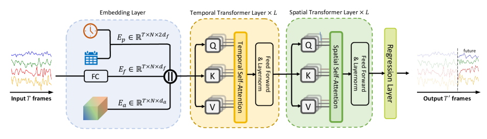
Figure 2. The Architecture of Spatio-Temporal Adaptive Embedding transformer (STAEformer).

3. Methodology

As shown in Figure 2, our model consists of an embedding layer, vanilla transformers applied along temporal axis as the temporal transformer layer and along spatial axis as the spatial transformer layer, then a regression layer. The embedding layer obtains the hidden representation fused by the feature embedding, the periodicity embedding, and the spatio-temporal adaptive embedding. The spatio-temporal transformer layers capture traffic relations, followed by a regression layer making the prediction.

3.1. Embedding Layer

To keep the native information in the raw data, we utilize a fully connected layer to obtain the feature embedding ${E_{f}}\in\mathbb{R}^{T\times N\times d_{f}}$:

(2) $$E_{f}=FC(X_{t-T+1:t})$$

where $d_{f}$ is the dimension of the feature embedding, and $FC(\cdot)$ indicates a fully connected layer.

We denote the learnable day-of-week embedding dict as $T_{w}\in\mathbb{R}^{N_{w}\times d_{f}}$, and the timestamps-of-day embedding dict as $T_{d}\in\mathbb{R}^{N_{d}\times d_{f}}$, where $N_{w}$ = 7 denotes the number of days in a week. In our case, $N_{d}$ = 288 is the number of timestamps in each day. Denoting $W^{t}\in\mathbb{R}^{T}$, $D^{t}\in\mathbb{R}^{T}$ as the day-of-week data and the timestamp-of-day data for the traffic time series in $t$-$T$+1:$t$, we use them as indices to extract the corresponding day-of-week embedding $E_{w}^{t}\in\mathbb{R}^{T\times d_{f}}$ and timestamp-of-day embedding $E^{t}_{d}\in\mathbb{R}^{T\times d_{f}}$ from the embedding dicts. By concatenating and broadcasting them, we get the periodicity embedding $E_{p}\in\mathbb{R}^{T\times N\times 2d_{f}}$ for the traffic time series.

On one hand, it’s intuitive that the temporal relation is not only decided by periodicity but also affected by the chronological order in the traffic time series. For example, a time frame in traffic time series should be more similar to the time frames nearby. On the other hand, the time series from different sensors tend to have different temporal patterns. Thus, instead of adopting a pre-defined or dynamic adjacency matrix for spatial relation modeling, we designed a spatio-temporal adaptive embedding $E_{a}\in\mathbb{R}^{T\times N\times d_{a}}$ to capture intricate spatio-temporal relation in a uniform way. In particular, $E_{a}$ is shared across different traffic time series.

By concatenating the embeddings above, we obtain the hidden spatio-temporal representation $Z\in\mathbb{R}^{T\times N\times d_{h}}$ as follows:

(3) $$Z=E_{f}||E_{p}||E_{a}$$

where the hidden dimension $d_{h}$ equals $3d_{f}+d_{a}$.

3.2. Transformer and Regression Layer

We apply vanilla transformers along temporal and spatial axes to capture intricate traffic relations.

Table 1. Performance on METR-LA and PEMS-BAY.

Datasets		Metric	HI	GWNet	DCRNN	AGCRN	STGCN	GTS	MTGNN	STNorm	GMAN	PDFormer	STID	STAEformer
METR-LA	Horizon 3 (15 min)	MAE	6.80	2.69	2.67	2.85	2.75	2.75	2.69	2.81	2.80	2.83	2.82	2.65
		RMSE	14.21	5.15	5.16	5.53	5.29	5.27	5.16	5.57	5.55	5.45	5.53	5.11
		MAPE	16.72%	6.99%	6.86%	7.63%	7.10%	7.12%	6.89%	7.40%	7.41%	7.77%	7.75%	6.85%
	Horizon 6 (30 min)	MAE	6.80	3.08	3.12	3.20	3.15	3.14	3.05	3.18	3.12	3.20	3.19	2.97
		RMSE	14.21	6.20	6.27	6.52	6.35	6.33	6.13	6.59	6.49	6.46	6.57	6.00
		MAPE	16.72%	8.47%	8.42%	9.00%	8.62%	8.62%	8.16%	8.47%	8.73%	9.19%	9.39%	8.13%
	Horizon 12 (60 min)	MAE	6.80	3.51	3.54	3.59	3.60	3.59	3.47	3.57	3.44	3.62	3.55	3.34
		RMSE	14.20	7.28	7.47	7.45	7.43	7.44	7.21	7.51	7.35	7.47	7.55	7.02
		MAPE	10.15%	9.96%	10.32%	10.47%	10.35%	10.25%	9.70%	10.24%	10.07%	10.91%	10.95%	9.70%
PEMS-BAY	Horizon 3 (15 min)	MAE	3.06	1.30	1.31	1.35	1.36	1.37	1.33	1.33	1.35	1.32	1.31	1.31
		RMSE	7.05	2.73	2.76	2.88	2.88	2.92	2.80	2.82	2.90	2.83	2.79	2.78
		MAPE	6.85%	2.71%	2.73%	2.91%	2.86%	2.85%	2.81%	2.76%	2.87%	2.78%	2.78%	2.76%
	Horizon 6 (30 min)	MAE	3.06	1.63	1.65	1.67	1.70	1.72	1.66	1.65	1.65	1.64	1.64	1.62
		RMSE	7.04	3.73	3.75	3.82	3.84	3.86	3.77	3.77	3.82	3.79	3.73	3.68
		MAPE	6.84%	3.73%	3.71%	3.81%	3.79%	3.88%	3.75%	3.66%	3.74%	3.71%	3.73%	3.62%
	Horizon 12 (60 min)	MAE	3.05	1.99	1.97	1.94	2.02	2.06	1.95	1.92	1.92	1.91	1.91	1.88
		RMSE	7.03	4.60	4.60	4.50	4.63	4.60	4.50	4.45	4.49	4.43	4.42	4.34
		MAPE	6.83%	4.71%	4.68%	4.55%	4.72%	4.88%	4.62%	4.46%	4.52%	4.51%	4.55%	4.41%

Given hidden spatio-temporal representation $Z\in\mathbb{R}^{T\times N\times d_{h}}$ with $T$ frames and $N$ spatial nodes, we obtain the query, key and value matrices through temporal transformer layers as:

(4) $$Q^{(te)}=ZW_{Q}^{(te)}\ ,\ K^{(te)}=ZW_{K}^{(te)}\ ,\ V^{(te)}=ZW_{V}^{(te)}$$

where $W_{Q}^{(te)},\ W_{K}^{(te)},\ W_{V}^{(te)}\ \in\mathbb{R}^{d_{h}\times d_{h}}$ are learable parameters. Then we calculate the self-attention score as:

(5) $$A^{(te)}=Softmax\left(\frac{Q^{(te)}{K^{(te)}}^{\top}}{\sqrt{d_{h}}}\right)$$

where $A^{(te)}\in\mathbb{R}^{N\times T\times T}$ captures the temporal relations in different spatial nodes. Finally, we obtain the output of temporal transformer $Z^{(te)}\in\mathbb{R}^{T\times N\times d_{h}}$ as:

(6) $$Z^{(te)}=A^{(te)}V^{(te)}.$$

Similarly, the spatial transformer layer performs as:

(7) $$Z^{(sp)}=SelfAttention(Z^{(te)})$$

where $SelfAttention$ follows Equation 4, 5, 6, and $Z^{(sp)}\in\mathbb{R}^{T\times N\times d_{h}}$ is the output of the spatial transformer. Notably, we also apply layer normalization, residual connection and multi-head mechanism.

Finally, we leverage the output of the spatio-temporal transformer layers $Z^{\prime}\in\mathbb{R}^{T\times N\times d_{h}}$ to generate predictions. The regression layer can be formulated as:

(8) $$\hat{Y}=FC(Z^{\prime})$$

where $\hat{Y}\in\mathbb{R}^{T^{\prime}\times N\times d}$ is the prediction, $T^{\prime}$ is the horizon of prediction. $d$ is the dimension of the output features which equals 1 in our case. Thus, the fully-connected layer regresses the dimension from $T\times d_{h}$ in $Z^{\prime}$ to $T^{\prime}\times(d=1)$ in $\hat{Y}$.

Table 2. Summary of Datasets.

Dataset	#Sensors (N)	#Timesteps	Time Range
METR-LA	207	34,272	03/2012 - 06/2012
PEMS-BAY	325	52,116	01/2017 - 05/2017
PEMS03	358	26,209	05/2012 - 07/2012
PEMS04	307	16,992	01/2018 - 02/2018
PEMS07	883	28,224	05/2017 - 08/2017
PEMS08	170	17,856	07/2016 - 08/2016

Table 3. Performance on PEMS03, 04, 07, and 08.

Dataset	PEMS03			PEMS04			PEMS07			PEMS08
Metric	MAE	RMSE	MAPE	MAE	RMSE	MAPE	MAE	RMSE	MAPE	MAE	RMSE	MAPE
HI	32.62	49.89	30.60%	42.35	61.66	29.92%	49.03	71.18	22.75%	36.66	50.45	21.63%
GWNet	14.59	25.24	15.52%	18.53	29.92	12.89%	20.47	33.47	8.61%	14.40	23.39	9.21%
DCRNN	15.54	27.18	15.62%	19.63	31.26	13.59%	21.16	34.14	9.02%	15.22	24.17	10.21%
AGCRN	15.24	26.65	15.89%	19.38	31.25	13.40%	20.57	34.40	8.74%	15.32	24.41	10.03%
STGCN	15.83	27.51	16.13%	19.57	31.38	13.44%	21.74	35.27	9.24%	16.08	25.39	10.60%
GTS	15.41	26.15	15.39%	20.96	32.95	14.66%	22.15	35.10	9.38%	16.49	26.08	10.54%
MTGNN	14.85	25.23	14.55%	19.17	31.70	13.37%	20.89	34.06	9.00%	15.18	24.24	10.20%
STNorm	15.32	25.93	14.37%	18.96	30.98	12.69%	20.50	34.66	8.75%	15.41	24.77	9.76%
GMAN	16.87	27.92	18.23%	19.14	31.60	13.19%	20.97	34.10	9.05%	15.31	24.92	10.13%
PDFormer	14.94	25.39	15.82%	18.36	30.03	12.00%	19.97	32.95	8.55%	13.58	23.41	9.05%
STID	15.33	27.40	16.40%	18.38	29.95	12.04%	19.61	32.79	8.30%	14.21	23.28	9.27%
STAEformer	15.35	27.55	15.18%	18.22	30.18	11.98%	19.14	32.60	8.01%	13.46	23.25	8.88%

4. Experiments

4.1. Experimental Setup

Datasets. Our method is verified on six traffic forecasting benchmarks, i.e., METR-LA, PEMS-BAY, PEMS03, PEMS04, PEMS07, and PEMS08. The first two datasets were proposed by DCRNN (Li et al., 2018). The last four datasets were proposed by STSGCN  (Song et al., 2020). The time interval in the six datasets is 5 minutes, so there are 12 frames in each hour. More details are shown in Table 2.

Implementation. We implement the model with the PyTorch toolkit on a Linux server with a GeForce RTX 3090 GPU. METR-LA and PEMS-BAY are divided into the training, validation, and test sets in a fraction of 7:1:2. PEMS03, PEMS04, PEMS07 and PEMS08 are divided in a fraction of 6:2:2. In fact, the performance of our model is not sensitive to the hyper-parameters. For more details, the embedding dimension $d_{f}$ is 24 and the $d_{a}$ is 80. The number of layers $L$ is 3 for both spatial and temporal transformers. The number of heads is 4. We set the input and prediction length to be 1 hour, namely, $T$=$T^{\prime}$=12. Adam is chosen as the optimizer with the learning rate decaying from 0.001, and the batch size is 16. We apply an early-stop mechanism if the validation error converges within 30 continuous steps. The code is available at https://github.com/XDZhelheim/STAEformer.

Table 4. Ablation Study on PEMS04, PEMS07 and PEMS08.

Dataset	PEMS04			PEMS07			PEMS08
Metric	MAE	RMSE	MAPE	MAE	RMSE	MAPE	MAE	RMSE	MAPE
w/o $E_{a}$	21.63	34.88	14.26%	22.37	37.21	9.25%	15.00	25.85	9.74%
w/o $E_{p}$	18.92	30.74	12.27%	20.21	33.59	8.40%	15.00	24.05	9.56%
w/o $T$-$Trans$	18.50	30.34	12.24%	19.87	33.67	8.29%	13.83	23.79	9.09%
w/o $ST$-$Trans$	25.17	39.89	18.00%	27.71	42.99	17.61%	19.96	31.47	18.53%
STAEformer	18.22	30.29	12.01%	19.14	32.60	8.01%	13.46	23.25	8.88%

Metrics. We use three widely used metrics for traffic forecasting task, i.e, MAE, RMSE and MAPE. Following previous work, we select the average performance of all predicted 12 horizons on the PEMS03, PEMS04, PEMS07 and PEMS08 datasets. To evaluate the METR-LA and PEMS-BAY datasets, we compare the performance on horizon 3, 6 and 12 (15, 30, and 60 min).

Baselines. In this study, we compare our proposed method against several widely used baselines in the field. HI (Cui et al., 2021) is a typical traditional model. We also consider STGNNs such as GWNet (Wu et al., 2019), DCRNN (Li et al., 2018), AGCRN (Bai et al., 2020), STGCN (Yu et al., 2018), GTS (Shang et al., 2021), and MTGNN (Wu et al., 2020), which employ the embeddings shown in Figure 1(a). Additionally, we examine STNorm (Deng et al., 2021), which focuses on factorizing traffic time series. While there exist Transformer-based methods for time series forecasting, such as Informer (Zhou et al., 2021), Pyraformer (Liu et al., 2021), FEDformer (Zhou et al., 2022), and Autoformer (Wu et al., 2021), they are not specially tailored for short-term traffic forecasting. Hence, we select GMAN (Zheng et al., 2020) and PDFormer (Jiang et al., 2023a), which are transformer models targeting the same task as ours. The input embeddings in  (Zheng et al., 2020) and  (Jiang et al., 2023a) follow the configuration in Figure 1(b). Furthermore, we consider STID (Shao et al., 2022b), which enhances the spaito-temporal distinction in traffic time series by utilizing the input embedding depicted in Figure 1(c).

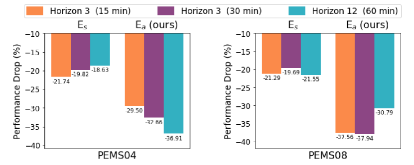
Figure 3. By shuffling the input along the temporal axis, our spatio-temporal adaptive embedding shows a more dramatic performance decrease than spatial embedding, indicating its capability in capturing chronological information.

4.2. Performance Evaluation

As shown in Table 1 and 3, our method achieves better performance on most metrics on all six datasets. STAEformer outperforms STGNNs by a large degree without any graph modeling. STNorm and STID also achieve competitive results, while Transformer-based models can better capture the intricate spatio-temporal relations. Compared with PDFormer, the encouraging results indicate STAEformer is a simpler but more effective solution.

4.3. Ablation Study

To evaluate the effectiveness of each part in STAEformer, we conduct ablation studies with 4 variants of our model as follows:

• w/o $E_{a}$. It removes spatio-temporal adaptive embedding $E_{a}$.

• w/o $E_{p}$. It removes periodicity embedding $E_{p}$, including day-of-week and timestamps-of-day embedding.

• w/o $T$-$Trans$. It removes temporal transformer layers.

• w/o $ST$-$Trans$. It removes both temporal transformer layers and spatial transformer layers.

Table 4 reveals the significance of various embeddings on the performance of our model. $E_{p}$ can capture daily and weekly patterns, while the proposed $E_{a}$ is vital for traffic modeling. Furthermore, the substantial performance degradation observed upon the removal of spatial or temporal transformer layers shows that our proposed embeddings effectively model the inherent spatio-temporal patterns in the traffic data. Therefore, both spatial and temporal layers are necessary for extracting those features.

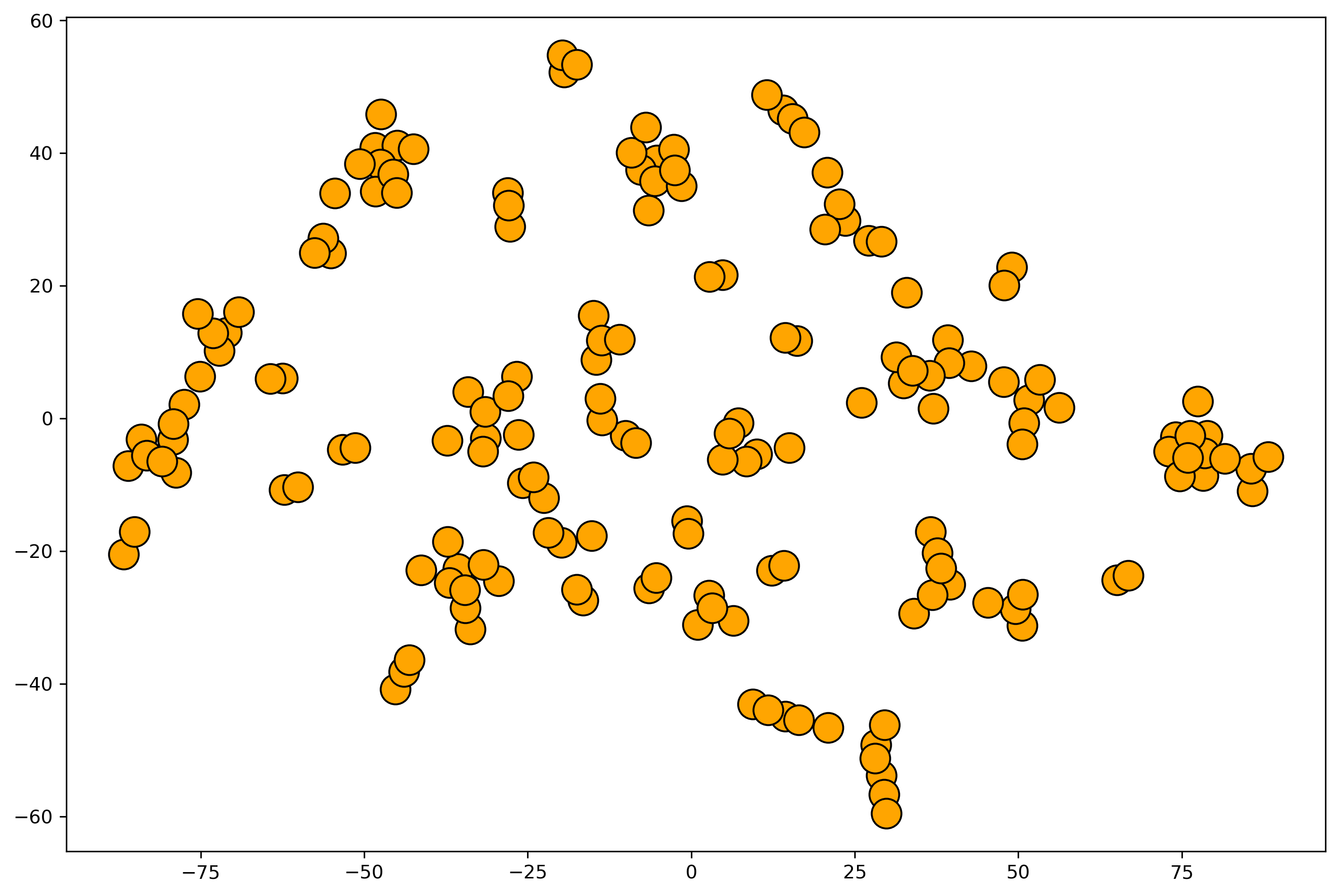
(a) Spatial Axis

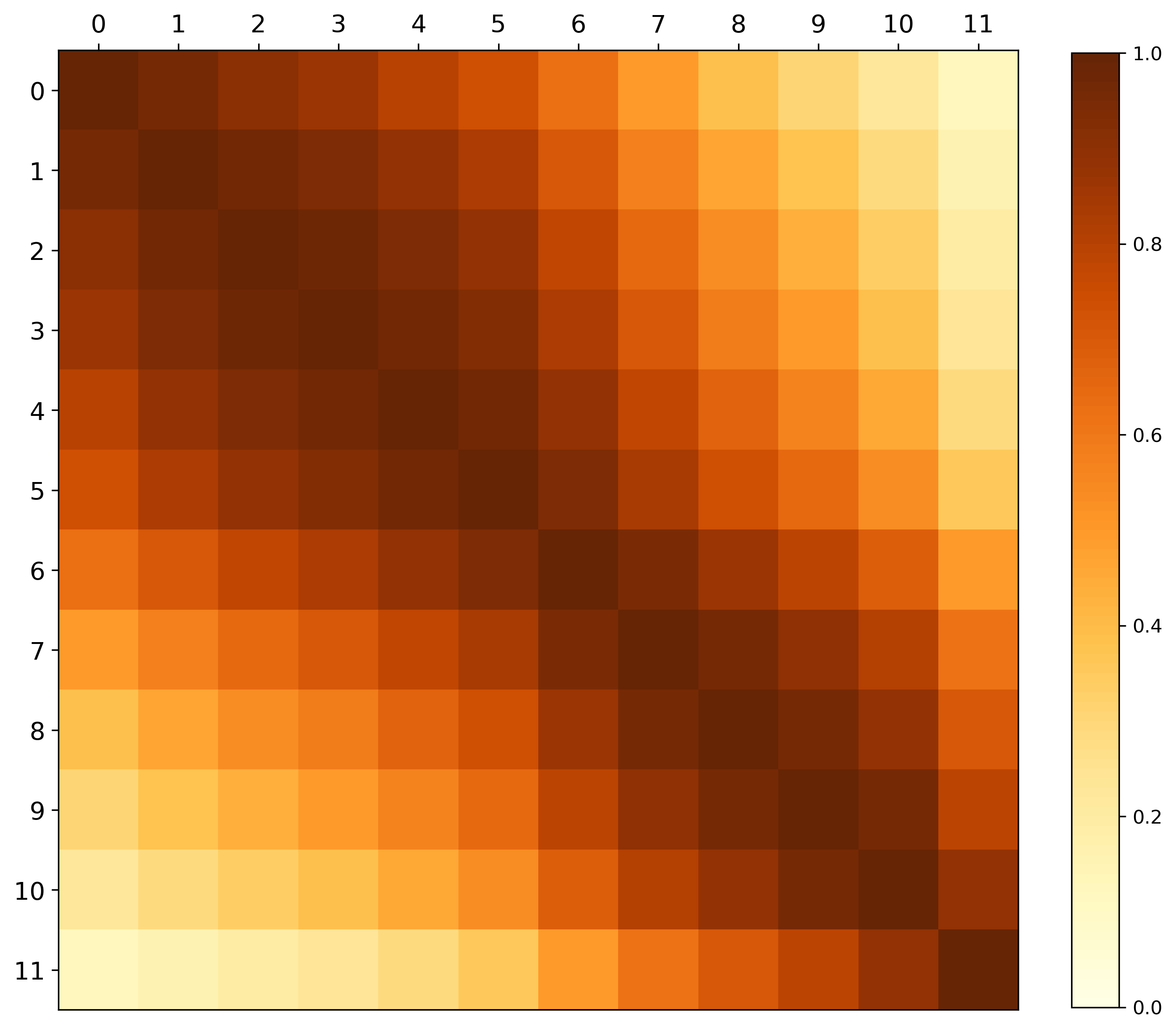
(b) Temporal Axis

Figure 4. Visualization of Spatio-Temporal Adaptive Embedding $E_{a}$ on PEMS08.

4.4. Case Study

Comparison with Spatial Embedding. To validate the effectiveness of spatio-temporal adaptive embedding in capturing chronological order information implied in the $T$ input frames, we conduct more experiments on PEMS04 and PEMS08 datasets. Following (Zeng et al., 2023), we randomly shuffle the raw input along temporal axis $T$. For comparison, we replace our spatio-temporal adaptive embedding $E_{a}$ with spatial embedding $E_{s}$ that was used in (Shao et al., 2022b; Jiang et al., 2023a). As shown by Figure 3, our model has more severe performance degradation when shuffling the raw input along temporal axis $T$. It means that spatio-temporal adaptive embedding $E_{a}$ makes our model more sensitive to the chronological order, while the model with $E_{s}$ is relatively insensitive. In summary, $E_{a}$ can better model the chronological information in the raw input and other intricate traffic patterns, which is crucial to the task.

Visualization of Spatio-Temporal Adaptive Embedding. Figure 4 further provides visualizations of our proposed spatio-temporal embedding $E_{a}$ on the spatial and temporal axes by taking PEMS08 dataset as an example. For the spatial axis, we use t-SNE (Van der Maaten and Hinton, 2008) to get Figure 4(a). It shows that the embeddings of different nodes naturally form into clusters, which matches the spatial characteristics of the traffic data. For the temporal axis, we calculate the correlation coefficient across the 12 input frames and draw a heat map as Figure 4(b). It shows that each frame is highly correlated to the nearby frames, and the correlation gradually decreases for further frames. This shows that our proposed $E_{a}$ models the chronological information in the time series correctly.

5. Conclusion

In this study, we focus on a basic representation learning technique for traffic time series forecasting, i.e., input embedding. We propose a novel spatio-temporal adaptive embedding that can work on vanilla transformers to achieve the SOTA performance on six traffic benchmarks. Further studies demonstrate that our model can effectively capture intrinsic spatio-temporal dependencies. Instead of designing complicated models, our study shows a promising direction for addressing the challenges in traffic forecasting.

- (1)
- Bai et al. (2020) Lei Bai, Lina Yao, Can Li, Xianzhi Wang, and Can Wang. 2020. Adaptive graph convolutional recurrent network for traffic forecasting. Advances in neural information processing systems 33 (2020), 17804–17815.
- Cao et al. (2020) Defu Cao, Yujing Wang, Juanyong Duan, Ce Zhang, Xia Zhu, Congrui Huang, Yunhai Tong, Bixiong Xu, Jing Bai, Jie Tong, et al. 2020. Spectral temporal graph neural network for multivariate time-series forecasting. Advances in neural information processing systems 33 (2020), 17766–17778.
- Chen et al. (2021) Yuzhou Chen, Ignacio Segovia-Dominguez, and Yulia R. Gel. 2021. Z-GCNETs: Time Zigzags at Graph Convolutional Networks for Time Series Forecasting. In ICML.
- Cirstea et al. (2021) Razvan-Gabriel Cirstea, Tung Kieu, Chenjuan Guo, Bin Yang, and Sinno Jialin Pan. 2021. EnhanceNet: Plugin neural networks for enhancing correlated time series forecasting. In 2021 IEEE 37th International Conference on Data Engineering (ICDE). IEEE, 1739–1750.
- Cirstea et al. (2022) Razvan-Gabriel Cirstea, Bin Yang, Chenjuan Guo, Tung Kieu, and Shirui Pan. 2022. Towards Spatio-Temporal Aware Traffic Time Series Forecasting–Full Version. arXiv preprint arXiv:2203.15737 (2022).
- Cui et al. (2021) Yue Cui, Jiandong Xie, and Kai Zheng. 2021. Historical inertia: A neglected but powerful baseline for long sequence time-series forecasting. In Proceedings of the 30th ACM International Conference on Information & Knowledge Management. 2965–2969.
- Deng et al. (2021) Jinliang Deng, Xiusi Chen, Renhe Jiang, Xuan Song, and Ivor W Tsang. 2021. St-norm: Spatial and temporal normalization for multi-variate time series forecasting. In Proceedings of the 27th ACM SIGKDD conference on knowledge discovery & data mining. 269–278.
- Diao et al. (2019) Zulong Diao, Xin Wang, Dafang Zhang, Yingru Liu, Kun Xie, and Shaoyao He. 2019. Dynamic spatial-temporal graph convolutional neural networks for traffic forecasting. In Proceedings of the AAAI conference on artificial intelligence, Vol. 33. 890–897.
- Fang et al. (2021) Zheng Fang, Qingqing Long, Guojie Song, and Kunqing Xie. 2021. Spatial-temporal graph ode networks for traffic flow forecasting. In Proceedings of the 27th ACM SIGKDD Conference on Knowledge Discovery & Data Mining. 364–373.
- Guo et al. (2021) Kan Guo, Yongli Hu, Yanfeng Sun, Sean Qian, Junbin Gao, and Baocai Yin. 2021. Hierarchical Graph Convolution Networks for Traffic Forecasting. In Proceedings of the AAAI Conference on Artificial Intelligence, Vol. 35. 151–159.
- Guo et al. (2019) Shengnan Guo, Youfang Lin, Ning Feng, Chao Song, and Huaiyu Wan. 2019. Attention based spatial-temporal graph convolutional networks for traffic flow forecasting. In Proceedings of the AAAI conference on artificial intelligence, Vol. 33. 922–929.
- Han et al. (2021) Liangzhe Han, Bowen Du, Leilei Sun, Yanjie Fu, Yisheng Lv, and Hui Xiong. 2021. Dynamic and Multi-faceted Spatio-temporal Deep Learning for Traffic Speed Forecasting. In Proceedings of the 27th ACM SIGKDD Conference on Knowledge Discovery & Data Mining. 547–555.
- Jiang et al. (2023a) Jiawei Jiang, Chengkai Han, Wayne Xin Zhao, and Jingyuan Wang. 2023a. PDFormer: Propagation Delay-aware Dynamic Long-range Transformer for Traffic Flow Prediction. In AAAI. AAAI Press.
- Jiang et al. (2023b) Renhe Jiang, Zhaonan Wang, Jiawei Yong, Puneet Jeph, Quanjun Chen, Yasumasa Kobayashi, Xuan Song, Shintaro Fukushima, and Toyotaro Suzumura. 2023b. Spatio-temporal meta-graph learning for traffic forecasting. In Proceedings of the AAAI Conference on Artificial Intelligence, Vol. 37. 8078–8086.
- Jiang et al. (2021) Renhe Jiang, Du Yin, Zhaonan Wang, Yizhuo Wang, Jiewen Deng, Hangchen Liu, Zekun Cai, Jinliang Deng, Xuan Song, and Ryosuke Shibasaki. 2021. Dl-traff: Survey and benchmark of deep learning models for urban traffic prediction. In Proceedings of the 30th ACM international conference on information & knowledge management. 4515–4525.
- Lee et al. (2022) Hyunwook Lee, Seungmin Jin, Hyeshin Chu, Hongkyu Lim, and Sungahn Ko. 2022. Learning to Remember Patterns: Pattern Matching Memory Networks for Traffic Forecasting. In International Conference on Learning Representations.
- Li and Zhu (2021) Mengzhang Li and Zhanxing Zhu. 2021. Spatial-Temporal Fusion Graph Neural Networks for Traffic Flow Forecasting. In Proceedings of the AAAI Conference on Artificial Intelligence, Vol. 35. 4189–4196.
- Li et al. (2018) Yaguang Li, Rose Yu, Cyrus Shahabi, and Yan Liu. 2018. Diffusion Convolutional Recurrent Neural Network: Data-Driven Traffic Forecasting. In International Conference on Learning Representations.
- Liu et al. (2021) Shizhan Liu, Hang Yu, Cong Liao, Jianguo Li, Weiyao Lin, Alex X Liu, and Schahram Dustdar. 2021. Pyraformer: Low-complexity pyramidal attention for long-range time series modeling and forecasting. In International conference on learning representations.
- Lu et al. (2020) Bin Lu, Xiaoying Gan, Haiming Jin, Luoyi Fu, and Haisong Zhang. 2020. Spatiotemporal adaptive gated graph convolution network for urban traffic flow forecasting. In Proceedings of the 29th ACM International conference on information & knowledge management. 1025–1034.
- Pan et al. (2021) Zheyi Pan, Songyu Ke, Xiaodu Yang, Yuxuan Liang, Yong Yu, Junbo Zhang, and Yu Zheng. 2021. AutoSTG: Neural Architecture Search for Predictions of Spatio-Temporal Graph. In Proceedings of the Web Conference 2021. 1846–1855.
- Pan et al. (2019) Zheyi Pan, Yuxuan Liang, Weifeng Wang, Yong Yu, Yu Zheng, and Junbo Zhang. 2019. Urban traffic prediction from spatio-temporal data using deep meta learning. In Proceedings of the 25th ACM SIGKDD International Conference on Knowledge Discovery & Data Mining. 1720–1730.
- Shang et al. (2021) Chao Shang, Jie Chen, and Jinbo Bi. 2021. Discrete Graph Structure Learning for Forecasting Multiple Time Series. In International Conference on Learning Representations.
- Shao et al. (2022b) Zezhi Shao, Zhao Zhang, Fei Wang, Wei Wei, and Yongjun Xu. 2022b. Spatial-temporal identity: A simple yet effective baseline for multivariate time series forecasting. In Proceedings of the 31st ACM International Conference on Information & Knowledge Management. 4454–4458.
- Shao et al. (2022a) Zezhi Shao, Zhao Zhang, Fei Wang, and Yongjun Xu. 2022a. Pre-training enhanced spatial-temporal graph neural network for multivariate time series forecasting. In Proceedings of the 28th ACM SIGKDD Conference on Knowledge Discovery and Data Mining. 1567–1577.
- Shao et al. (2022c) Zezhi Shao, Zhao Zhang, Wei Wei, Fei Wang, Yongjun Xu, Xin Cao, and Christian S Jensen. 2022c. Decoupled dynamic spatial-temporal graph neural network for traffic forecasting. Proceedings of the VLDB Endowment 15, 11 (2022), 2733–2746.
- Song et al. (2020) Chao Song, Youfang Lin, Shengnan Guo, and Huaiyu Wan. 2020. Spatial-temporal synchronous graph convolutional networks: A new framework for spatial-temporal network data forecasting. In Proceedings of the AAAI conference on artificial intelligence, Vol. 34. 914–921.
- Van der Maaten and Hinton (2008) Laurens Van der Maaten and Geoffrey Hinton. 2008. Visualizing data using t-SNE. Journal of machine learning research 9, 11 (2008).
- Vaswani et al. (2017) Ashish Vaswani, Noam Shazeer, Niki Parmar, Jakob Uszkoreit, Llion Jones, Aidan N Gomez, Łukasz Kaiser, and Illia Polosukhin. 2017. Attention is all you need. Advances in neural information processing systems 30 (2017).
- Wang et al. (2022) Chunnan Wang, Kaixin Zhang, Hongzhi Wang, and Bozhou Chen. 2022. Auto-STGCN: Autonomous Spatial-Temporal Graph Convolutional Network Search. ACM Transactions on Knowledge Discovery from Data (2022).
- Wang et al. (2020) Xiaoyang Wang, Yao Ma, Yiqi Wang, Wei Jin, Xin Wang, Jiliang Tang, Caiyan Jia, and Jian Yu. 2020. Traffic flow prediction via spatial temporal graph neural network. In Proceedings of the web conference 2020. 1082–1092.
- Wu et al. (2021) Haixu Wu, Jiehui Xu, Jianmin Wang, and Mingsheng Long. 2021. Autoformer: Decomposition transformers with auto-correlation for long-term series forecasting. Advances in Neural Information Processing Systems 34 (2021), 22419–22430.
- Wu et al. (2020) Zonghan Wu, Shirui Pan, Guodong Long, Jing Jiang, Xiaojun Chang, and Chengqi Zhang. 2020. Connecting the dots: Multivariate time series forecasting with graph neural networks. In Proceedings of the 26th ACM SIGKDD international conference on knowledge discovery & data mining. 753–763.
- Wu et al. (2019) Zonghan Wu, Shirui Pan, Guodong Long, Jing Jiang, and Chengqi Zhang. 2019. Graph wavenet for deep spatial-temporal graph modeling. In Proceedings of the 28th International Joint Conference on Artificial Intelligence. 1907–1913.
- Xu et al. (2020) Mingxing Xu, Wenrui Dai, Chunmiao Liu, Xing Gao, Weiyao Lin, Guo-Jun Qi, and Hongkai Xiong. 2020. Spatial-temporal transformer networks for traffic flow forecasting. arXiv preprint arXiv:2001.02908 (2020).
- Ye et al. (2021) Junchen Ye, Leilei Sun, Bowen Du, Yanjie Fu, and Hui Xiong. 2021. Coupled Layer-wise Graph Convolution for Transportation Demand Prediction. In Proceedings of the AAAI Conference on Artificial Intelligence, Vol. 35. 4617–4625.
- Yu et al. (2018) Bing Yu, Haoteng Yin, and Zhanxing Zhu. 2018. Spatio-temporal graph convolutional networks: a deep learning framework for traffic forecasting. In Proceedings of the 27th International Joint Conference on Artificial Intelligence. 3634–3640.
- Zeng et al. (2023) Ailing Zeng, Muxi Chen, Lei Zhang, and Qiang Xu. 2023. Are Transformers Effective for Time Series Forecasting? Proceedings of the AAAI Conference on Artificial Intelligence.
- Zhang et al. (2020) Qi Zhang, Jianlong Chang, Gaofeng Meng, Shiming Xiang, and Chunhong Pan. 2020. Spatio-temporal graph structure learning for traffic forecasting. In Proceedings of the AAAI conference on artificial intelligence, Vol. 34. 1177–1185.
- Zhao et al. (2019) Ling Zhao, Yujiao Song, Chao Zhang, Yu Liu, Pu Wang, Tao Lin, Min Deng, and Haifeng Li. 2019. T-gcn: A temporal graph convolutional network for traffic prediction. IEEE Transactions on Intelligent Transportation Systems 21, 9 (2019), 3848–3858.
- Zheng et al. (2020) Chuanpan Zheng, Xiaoliang Fan, Cheng Wang, and Jianzhong Qi. 2020. Gman: A graph multi-attention network for traffic prediction. In Proceedings of the AAAI conference on artificial intelligence, Vol. 34. 1234–1241.
- Zhou et al. (2021) Haoyi Zhou, Shanghang Zhang, Jieqi Peng, Shuai Zhang, Jianxin Li, Hui Xiong, and Wancai Zhang. 2021. Informer: Beyond efficient transformer for long sequence time-series forecasting. In Proceedings of the AAAI conference on artificial intelligence, Vol. 35. 11106–11115.
- Zhou et al. (2022) Tian Zhou, Ziqing Ma, Qingsong Wen, Xue Wang, Liang Sun, and Rong Jin. 2022. Fedformer: Frequency enhanced decomposed transformer for long-term series forecasting. In International Conference on Machine Learning. PMLR, 27268–27286.