Integrated Sensing and Communications
for 3D Object Imaging via Bilinear Inference

Abstract

We consider an uplink integrated sensing and communications (ISAC) scenario where the detection of data symbols from multiple user equipment (UEs) occurs simultaneously with a three-dimensional (3D) estimation of the environment, extracted from the scattering features present in the channel state information (CSI) and utilizing the same physical layer communications air interface, as opposed to radar technologies. By exploiting a discrete (voxelated) representation of the environment, two novel ISAC schemes are derived with purpose-built message passing (MP) rules for the joint estimation of data symbols and status (filled/empty) of the discretized environment. The first relies on a modular feedback structure in which the data symbols and the environment are estimated alternately, whereas the second leverages a bilinear inference framework to estimate both variables concurrently. Both contributed methods are shown via simulations to outperform the state-of-the-art (SotA) in accurately recovering the transmitted data as well as the 3D image of the environment. An analysis of the computational complexities of the proposed methods reveals distinct advantages of each scheme, namely, that the bilinear solution exhibits a superior robustness to short pilots and channel blockages, while the alternating solution offers lower complexity with large number of UEsand superior performance in ideal conditions.

I Introduction

Beyond fifth-generation (B5G) and sixth-generation (6G) wireless communication systems are expected to raise the performance standards in terms of data throughput, reliability, latency, spectral efficiency, energy efficiency, and user capacity [4, 5, 6], which can be achieved by novel enabling technologies such as high-frequency communications in the millimeter-wave (mmWave) [7, 8, 9] and Terahertz (THz) [10, 11, 12] bands, massive multiple-input multiple-output (mMIMO) techniques [13, 14, 15], reconfigurable intelligent surfaces (RISs) [16, 17, 18], and more.

Within that context, a new research field called integrated sensing and communications (ISAC) [19, 20, 21], also known as joint communication and sensing (JCAS) [22, 23, 24, 25, 26], has recently gained significant attention as a promising technology to fulfill such requirements and enable new applications for B5G and 6G systems. In particular, ISAC technology seeks to enhance B5G and 6G systems by enabling both communication and environment sensing functionalities under the same wireless interface, thus realizing the concepts of ambient-sensing and environment-aware radio [27], which are crucial to emerging applications such as autonomous driving (AD) [28] and drone networking (DN) [29], besides offering new means to optimize system performance. For instance, in B5G and 6G systems operating at high-frequency channels, which are sensitive to path-dependent scattering [30, 31], environment parameters of interest include not only the “usual” channel state information (CSI), but also the positions of users and obstacles that may lead to path blockages. In such systems, ISAC is an alternative to image-based path-blockage prediction approaches, crucial to mitigate the deleterious effects of blockages [32, 33, 34].

The prominent challenge of ISAC arises from the fact that two independently-developed wireless technologies, namely, wireless communications and radar systems [35, 36], are both fundamentally based on distinct air-interfaces, such that a concurrent deployment of existing waveforms is bound to suffer from performance degradation of both functions due to interference. Aiming to frontally address this issue, the earliest family of ISAC approaches known as the radar and communication coexistence (RCC) [37, 38], consequently focused on minimizing the interference and maximizing the cooperation between the independently-operated communications and radar subsystems sharing the same frequency spectrum. While the RCC strategy addresses succeeds in managing interference and harmoniously allocating radio resources to operate both subsystems, the approach achieves relatively low spectral efficiencies and does not alleviate hardware costs, whose components remain separate for both subsystems [37, 25, 38].

In light of the fundamental drawbacks of RCC, techniques integrating the communication and radar functions into a single wireless interface have been recently proposed to truly realize the ISAC goal of jointly offering communication and sensing capabilities in a single system. Literature [24, 25, 26] classifies such techniques into three types: a) Radar-centric ISAC (RC-ISAC) schemes, which realizes an additional communication functionality over typical radar waveforms, for example by utilizing index modulation (IM) to encode information into multiple-input multiple-output (MIMO) radar signals employing, e.g., the carrier agile phased array radar (CAESAR) waveform [39], or the frequency modulated continuous waveforms (FMCW) [40]; b) Communication-centric ISAC (CC-ISAC) schemes, which realizes an additional environment sensing functionality over standard communication waveforms, typically by extracting the radar parameters such as Doppler-shift and delay from waveforms designed fundamentally for communications functions, such as the IEEE 802.11ad waveform [41], the orthogonal frequency-division multiplex (OFDM) waveform [42], or the orthogonal time frequency space (OTFS) waveform [43]; and c) Dual-function radar communications (DFRC) schemes, which while not having exclusive boundaries with aforementioned RC-ISAC and CC-ISAC categories, are based on waveforms that can be adaptively or jointly optimized between the two functionalities [44], e.g., via waveforms designed based on mutual information [45] or the multi-beam approach in the mmWave bands [46]. But still, all these approaches are related by the fact that the target sensing is enabled by the fundamental radar relationship between measurable physical quantities and information on the target [35, 36], that is, target range can be extracted from the delay in the signal, velocity from the Doppler frequency, and bearing from the angle-of-arrival (AoA).

Concomitant with the aforementioned methods, contributions have also been recently made to realize environment sensing capabilities not via target detection with radar, but rather by new standards of environment sensing information such as ambient human activity [47, 48], and three-dimensional (3D) environment image [49, 50, 51]. In particular, the latter family of works exploit the voxelated occupancy grid [52, 53, 54, 55] to discretize the environment into 3D cubic units of space representing its state (solid or void). Such methods exhibit a unique advantage in that the extracted information not only describes the location of objects, but also their 3D shape and orientation, in any desired resolution according to the voxelated model, enabling useful applications such as 3D environment mapping and ray-tracing propagation modeling [56, 57].

However, wireless voxelated imaging technology is still a very new notion in context of ISAC, due to the inherently convoluted channel paths arising from the discretization of the environment scatterers, and the fundamental challenge that the unknown information symbols must be simultaneously recovered on top of the very large number of environment voxels.

In light of the above challenges, we offer in this article the following contributions:

• An extension of the discrete voxelated environment model utilized in [49, 50, 51] is introduced, in which an empirical stochastic-geometric approach is incorporated to capture the viability of non-line-of-sight (NLOS) paths, in addition to an extension where the occupancy coefficients are not limited to 0 or 1, but instead can take on non-binary complex values, enabling reflection losses and phase shifts of reflected waves to be modeled.

• A novel, scalable CC-ISAC scheme is proposed, in which the 3D voxelated environment image and the transmit symbols are estimated alternately via two distinct linear modules;

• A novel, high-performance CC-ISAC scheme is proposed, in which the the 3D voxelated image of the environment and the transmit data symbols are concurrently estimated via a single message passing (MP) module which leverages a bilinear inference framework;

• Insights on the advantages of the two proposed CC-ISAC algorithms are provided via performance assessment and comparison against the state-of-the-art (SotA), which highlights the robustness of the bilinear method against short pilot lengths and path blockages, and the accuracy of the alternating solution in systems with many user equipment (UEs).

Notation: Scalar values are denoted by slanted lowercase letters, as in $x$, while complex vectors and matrices are denoted by boldface lowercase and uppercase letters, as in $\mathbf{x}$ and $\mathbf{X}$, respectively. The transposition, complex conjugation, diagonalization, absolute value, and $\ell$-th norm operators are denoted by $(\cdot)^{\mathsf{T}}$, $(\cdot)^{*}$, ${\mathrm{diag}}\!\left({\cdot}\right)$, $|\cdot|$, and $||\cdot||_{\ell}$ respectively, while $\mathbb{E}_{\mathsf{x}}(x)$ and $\mathrm{Var}_{\mathsf{x}}(x)$ respectively denote the expectation and variance of $x$ with respect to its distribution $\mathbb{P}_{\mathsf{x}}(x)$. The sets of real and complex numbers are denoted by $\mathbb{R}$ and $\mathbb{C}$, respectively, and $\mathcal{N}(\mu,\nu)$ and $\mathcal{CN}(\mu,\nu)$ denote the real and complex Normal distributions with mean $\mu$ and variance $\nu$.

II System Model

The system model considered throughout the article, consists of three parts: a) the environment model, where a voxelated occupancy grid is used to discretely approximate the true environment and its scattering properties, b) the channel model, which defines the unique channel paths arising from the voxelated environment model, and c) the signal model, where the uplink communication scheme between the UEs and the access points (APs) is described.

II-A Environment Voxelation Model

The 3D image of an environment can be represented via a number of techniques, including the well-known point-cloud and the ray-tracing methods, which are often utilized in robotics, machine vision and computer graphics [56, 58]. Another well-known method, however, is the voxelated occupancy grid [52, 53, 54, 55], where the region of interest (ROI) is represented as a cuboidal space of dimensions $L_{\mathrm{x}}\times L_{\mathrm{y}}\times L_{\mathrm{z}}$, each denoting the lengths of the $\mathrm{x},\mathrm{y},\mathrm{z}$-axes in meters, respectively, as depicted in Figure 1. In this model, the ROI is subdivided into a regular grid consisting of $N_{V}\triangleq N_{\mathrm{x}}\cdot N_{\mathrm{y}}\cdot N_{\mathrm{z}}$ voxels, where $N_{\mathrm{x}}\triangleq\frac{L_{\mathrm{x}}}{L_{V}}$, $N_{\mathrm{y}}\triangleq\frac{L_{\mathrm{y}}}{L_{V}}$, and $N_{\mathrm{z}}\triangleq\frac{L_{\mathrm{z}}}{L_{V}}$ denote the number of partitions along the $\mathrm{x},\mathrm{y}$ and $\mathrm{z}$-axes, respectively, and $L_{V}$ is the edge length of a voxel in meters, which therefore corresponds to the image resolution.

The environment is then represented by a 3D tensor of dimensions ($N_{\mathrm{x}}\times N_{\mathrm{y}}\times N_{\mathrm{z}}$), whose elements indicate the occupancy of the voxels, and thus whether that portion of the space is empty or filled with a given material. One may therefore consider, in general, each $k$-th voxel to be represented by an occupancy (a.k.a. scattering) coefficient $v_{k}$, with $k\in\{1,\cdots,N_{V}\}$, where $v_{k}=0$ indicates that the $k$-th voxel is empty, while an occupied voxel is indicated by a complex number i.e., $v_{k}\triangleq\beta_{k}\cdot e^{-j\omega_{k}}\in\mathbb{C}$. In such a model, the constants $\beta_{k}$ and $\omega_{k}$, which dependent not only on the material itself, but also on the frequency and the angle of incidence of propagating signals [31], capture the effect of the material occupying a given voxel onto the electromagnetic wave reflected or refracted by it. For the sake of reducing the complexity of the ISAC algorithm to be later introduced, however, we will in this article consider a simplified model whereby the occupancy coefficients $v_{k}$ take on discrete real values in the interval $\in[0,1]$.

Since phase rotations due to reflections are captured by channel estimation, this simplification is equivalent to the assumptions that the ISAC waveform is narrowband, so that frequency-dependence can be ignored [31]. The incorporation of the geometry of the interaction between propagating waves and occupied voxels will be described in Subsection II-C.

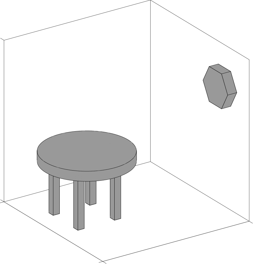
(a) True environment ROI.

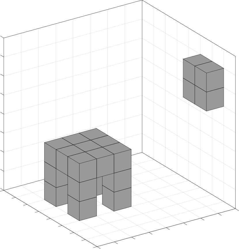
(b) Low resolution ROI model.

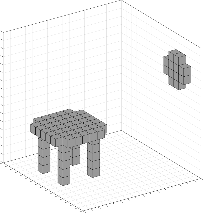
(c) High resolution ROI model.

Figure 1: Illustration of a voxelated grid map-based model of the environment of a given ROI.

II-B Channel Model

Consider a scenario in which the ROI contains $N_{U}$ single-antenna UEs, and $N_{A}$ multi-antenna APs equipped with $N_{R}$ receive antennas each. As illustrated in Fig. 2, the effective channels between the UEs and APs contain two distinct types of components, namely, line-of-sight (LOS) components which are direct paths between the UEs and APs, and NLOS components which encompass paths reflected at occupied voxels corresponding to parts of the environment, as described in Subsection II-A. Assuming that the operating frequency band is sufficiently high that the power of paths reflected more than once is negligible [30, 59], NLOS components may be decomposed into two subpaths, the UE-to-voxel subpath and the voxel-to-AP subpath, which together with the voxel scattering coefficient comprises the aggregate NLOS channel.

In light of the above, the effective channel between the $N_{U}$ single-antenna UEs and the ensemble of $N_{A}N_{R}$ receive antennas of all APscan be compactly described by

$$\mathbf{G}=\overbrace{\mathbf{H}}^{\text{UE-to-AP}}+\overbrace{\mathbf{A}}^{\text{voxel-to-AP}}\cdot\hskip 2.15277pt\mathrm{diag}({\mathbf{v}})\cdot\overbrace{\mathbf{B}}^{\text{UE-to-voxel}}\in\mathbb{C}^{N_{A}N_{R}\times N_{U}},\vspace{-1ex}$$ (1)

where $\mathbf{G}\in\mathbb{C}^{N_{A}N_{R}\times N_{U}}$ is the effective channel matrix, $\mathbf{H}\in\mathbb{C}^{N_{A}N_{R}\times N_{U}}$, $\mathbf{A}\in\mathbb{C}^{N_{A}N_{R}\times N_{V}}$, and $\mathbf{B}\in\mathbb{C}^{N_{V}\times N_{U}}$ are the channel matrices of the UE-to-AP LOS path, voxel-to-AP NLOS subpath, and UE-to-voxel NLOS subpath, respectively, whose elements are assumed to follow zero-mean complex Normal distributions with variances $\sigma_{H}^{2},\sigma_{A}^{2}$, and $\sigma_{B}^{2}$, respectively; while $\mathbf{v}\in\mathbb{C}^{N_{V}\times 1}$ is the vector containing all scattering coefficients of the voxelated grid.

Although not further exploited in this article, we emphasize that the channel model in equation (1) can be straightforwardly extended to a multi-carrier scenario by simply introducing frequency-selectivity such that the environment variables are functions of the carrier frequency, i.e.,

$$\mathbf{G}(f)=\mathbf{H}(f)+\mathbf{A}(f)\cdot{\mathrm{diag}}\!\left({\mathbf{v}(f)}\right)\cdot\mathbf{B}(f)~{}\forall f\in\mathcal{F},\vspace{-1ex}$$ (2)

with $f$ denoting a specific frequency in the set $\mathcal{F}$ of all subcarrier frequencies.

We leave details for follow-up work, but it shall become evident that under such an extended model, the sensing component of the ISAC algorithm to be introduced in Section III can also be extended for even better performance, for instance by exploiting knowledge of channel correlation across carriers [60], and to incorporate additional features, such as the estimation of material types based on the frequency-dependence observed on estimated scattering coefficients [31]. Since the above also requires incorporating message-passing rules that exploit cross-carrier correlation to the algorithms, such extension will be pursued in a future work, and only the frequency-independent ($i.e.$, single-carrier) model of equation (1) will be assumed in this article.

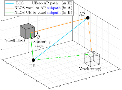
Figure 2: Illustration of the LOS and NLOS channel components and their subpaths.

II-C Stochastic Geometric Environment Model

Notice that the channel model summarized by equation (1) implies that all paths between UEs, APs, and voxels are available. Although such an assumption is common in related literature (see $e.g.$ [49, 50, 51, 52, 53, 54, 55]), in practice, many subpaths may not be available due to either physical phenomena ($e.g.$ blockage by air-borne particles, absorption, or path loss) or the finite resolution of the voxelated model itself. In order to capture such realistic behavior, the work in [51] considers the occlusion effect of waves reaching the voxels, where the UE-to-voxel subpaths are assumed to be unavailable if a voxel is present nearby the path. This perturbation effect was approximated by applying a 3D Gaussian kernel convolution to the channel matrix, but it was acknowledged [51] that this approach is a highly simplified model of the true physical phenomena. Building on the latter, we therefore seek to contribute to improving the voxelated grid model by considering the statistical feasibility of paths.

To this end, we refer to the physical phenomena occurring at the reflection of propagating waves, in particular, the fact that for any given frequency: a) a critical angle $\theta^{*}$ exists such that, as illustrated in Fig. 3(a), if the incidence angle $\theta>\theta^{*}$, the wave is absorbed rather than reflected, and consequently the corresponding voxel-to-AP NLOS subpath is not available [31]; and b) the curvature of the surface exposed to the impinging wave may be such that no signal is reflected towards an AP [52], as illustrated in Fig. 3(b). But since the complexity of modeling such phenomena at each voxel is far too complex to carry out, especially if the resolution of the voxelated ROI is large, we instead employ a statistical approach whereby the angle between the impinging and reflected waves at each voxel, hereafter referred to as the scattering angle, and consequently, the availability of each voxel-to-AP NLOS subpath, are considered.

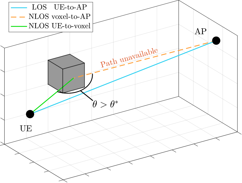
(a) Path unavailability due to obtuse scattering.

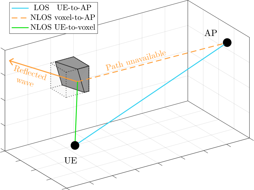
(b) Path unavailability due to skewed surface.

Figure 3: Illustration of physical phenomena leading to the unavailability of propagation paths.

In light of the above, the following stochastic-geometric model is proposed to integrate the aforementioned phenomena into the channel matrices of the voxelated grid environment model. First, the positions of the UEs and the APs are discretized into the 3D grid of the voxelated ROI, such that their positions may be described by voxel coordinates Denoting the 3D coordinates of an UE, an AP, and an environment voxel, respectively by $\mathbf{c}_{U}=[x_{U},y_{U},z_{U}]^{\mathsf{T}}\in\mathbb{R}^{3}$, $\mathbf{c}_{A}=[x_{A},y_{A},z_{A}]^{\mathsf{T}}\in\mathbb{R}^{3}$, and $\mathbf{c}_{V}=[x_{V},y_{V},z_{V}]^{\mathsf{T}}\in\mathbb{R}^{3}$, the scattering angle $\theta$ of the NLOS path reflected at the voxel is given by

$$\theta=\mathrm{arccos}\!\left(\dfrac{(\mathbf{c}_{U}-\mathbf{c}_{V})^{\mathsf{T}}(\mathbf{c}_{A}-\mathbf{c}_{V})}{||\mathbf{c}_{U}-\mathbf{c}_{V}||\!\cdot\!||\mathbf{c}_{A}-\mathbf{c}_{V}||}\right)\in[0,\pi],$$ (3)

where $\mathrm{arccos}(\cdot)$ denotes the inverse cosine trigonometric function.

The empirical ​​ probability distribution functions (PDFs) of the scattering angles $\theta$ can be obtained by evaluating equation (3) for all possible combinations of admissible locations of UE, AP and voxel within the ROI, respectively given by $\mathbf{c}_{U}$, $\mathbf{c}_{A}$ and $\mathbf{c}_{V}$, and examples of the latter for an environment voxelated at various resolutions are shown in Fig. 4.

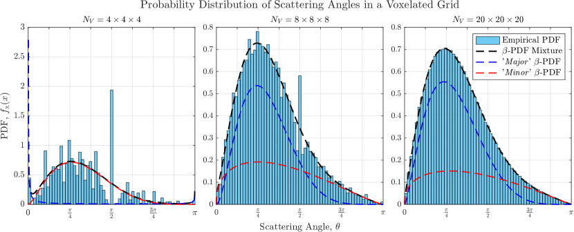
Figure 4: Empirical beta mixture modeling of scattering angle distributions.

It is visible in Figure 4 that for a sufficiently large $N_{V}$, the distribution of scattering angles $\theta$ can be well modeled by a mixture of two scaled beta distributions, namely, ${f}_{\mathrm{x}}(x)=\gamma\!\cdot\!\beta(a_{1},b_{1})+(1-\gamma)\!\cdot\!\beta(a_{2},b_{2})$, with support $x\in[0,\pi]$ and where $\gamma$ is a weighing factor and the quantities $a_{1},a_{2},b_{1},b_{2}$ are shape parameters optimised to match the empirical data obtained by evaluating equation (3), with $\mathbf{c}_{U}$, $\mathbf{c}_{A}$ and $\mathbf{c}_{V}$ taken randomly within the voxelated grid.

Utilizing this empirical stochastic-geometric approach, the increasingly popular voxelated model utilized in various related works [49, 50, 51, 53, 54, 55] can be improved by the incorporation of random blockages of NLOS subpaths, in proportion to the complement cumulative distribution of the approximated beta mixture PDF, and in accordance to the scattering angles at each voxel, as a function of a selected critical angle.

II-D Signal Model

Consider an uplink communication scenario between the group of $N_{U}$ UEs and a total of $N_{A}$ APs, under the models described above in Subsections II-A through II-C, with the $N_{A}$ APs connected to a central processing unit (CPU) via error-free fronthaul links of unlimited throughput, such that the received signals at all $N_{A}N_{R}$ receive antennas are aggregated without loss of information or delay.

Then, the aggregated received signal matrix $\mathbf{Y}$, over $N_{T}$ discrete transmission instances (symbol slots) is given by

$$\mathbf{Y}=\mathbf{G}\mathbf{X}+\mathbf{W}\in\mathbb{C}^{N_{A}N_{R}\times N_{T}},\vspace{-1.5ex}$$ (4)

where $\mathbf{G}\in\mathbb{C}^{N_{A}N_{R}\times N_{U}}$ is the effective channel matrix as described in Subsection II-B; $\mathbf{X}\in\mathbb{C}^{N_{U}\times N_{T}}$ is the transmit signal matrix collecting the symbols from all $N_{U}$ UEs, each drawn from the constellation $\mathcal{X}$ of cardinality $N_{\mathcal{X}}$; and $\mathbf{W}\in\mathbb{C}^{N_{A}N_{R}\times N_{T}}$ is the receive additive white Gaussian noise (AWGN) matrix with independent and identically distributed (i.i.d.) elements drawn from $\mathcal{CN}(0,N_{0})$, where $N_{0}$ is the noise variance.

The transmit signal $\mathbf{X}$ comprises of a pilot block $\mathbf{X}_{P}\in\mathbb{C}^{N_{U}\times N_{P}}$ and a data block $\mathbf{X}_{D}\in\mathbb{C}^{N_{U}\times N_{D}}$, such that

$$\begin{matrix}\mathbf{X}\end{matrix}=\begin{bmatrix}\mathbf{X}_{P}&\!\mathbf{X}_{D}\end{bmatrix}\begin{matrix}\in\mathbb{C}^{N_{U}\times N_{T}},\end{matrix}\vspace{-1ex}$$ (5)

where $N_{P}$ and $N_{D}$ denote the number of symbol slots allocated to the pilot and data sequences, respectively, with $N_{T}=N_{P}+N_{D}$; and where the pilot symbol matrix $\mathbf{X}_{P}$ is assumed to be perfectly known at the CPU.

In view of equations (1), (4) and (5), the goal of the ISAC schemes to be hereafter presented can be concisely stated. The communication objective of the CPU is to estimate the unknown data symbol matrix $\mathbf{X}_{D}$, under the knowledge of only the pilot symbols in $\mathbf{X}_{P}$, after the estimation of the channel matrix $\mathbf{G}$. In turn, the sensing objective is to extract the voxelated model of the environment as the vector of occupancy coefficients $\mathbf{v}$, from the said channel matrix $\mathbf{G}$.

III Proposed ISAC Solution

By combining the channel decomposition model of equation (1), the received signal model of equation (4), and the transmit signal in model of equation (5), the overall system model becomes

$$\mathbf{Y}=\overbrace{\big{(}\mathbf{H}+\mathbf{A}{\mathrm{diag}}\!\left({\mathbf{v}}\right)\!\mathbf{B}\big{)}}^{\triangleq\mathbf{G}}\overbrace{\big{[}\mathbf{X}_{P}\;\mathbf{X}_{D}\big{]}}^{\triangleq\mathbf{X}}+\mathbf{W}\in\mathbb{C}^{N_{A}N_{R}\times N_{T}},\vspace{-1.5ex}$$ (6)

where the unknown variables of interest are the environment (voxel coefficients) vector $\mathbf{v}$ and the data symbol matrix $\mathbf{X}_{D}$.

Similar to related literature [49, 50, 51, 53, 54, 55], it is assumed hereafter that the LOS channel $\mathbf{H}$, and the UE-to-voxel and voxel-to-AP subpath of components $\mathbf{A}$ and $\mathbf{B}$ in equation (6) are known, which still leaves an atypical relationship between the two variables ${\mathrm{diag}}\!\left({\mathbf{v}}\right)$ and $\mathbf{X}_{D}$. In particular, the latter unknowns are related, under equation (6), by an asymmetric bilinear system, requiring sophisticated algorithms to be either decoupled or jointly estimated [63, 64, 65, 66, 67, 68].

In light of the above, we propose in the sequel two novel ISAC solutions for the joint estimation problem of the asymmetric bilinear system expressed by (6), by leveraging the Gaussian belief propagation (GaBP) MP framework. The first proposed method incorporates two separate linear estimation modules for each of the unknown variables $\mathbf{v}$ and $\mathbf{X}_{D}$, estimating them in an alternate fashion via feedback between the two modules. In turn, the second method utilizes only a single bilinear estimation module which enables the simultaneous extraction of both unknown variables.

III-A Proposed Alternating Linear ISAC Algorithm (AL-ISAC)

The first proposed method, dubbed the “Alternating Linear ISAC (AL-ISAC)” algorithm, leverages two separate linear GaBP MP modules based on equation (6), which are respectively described as: 1) a linear GaBP module to estimate the environment vector $\mathbf{v}$, given the transmit signal $\mathbf{X}$, and conversely; and 2) a linear GaBP module to estimate the transmit signal matrix $\mathbf{X}$, given the environment vector $\mathbf{v}$.

The two linear GaBP modules and the constituting MP rules are derived in the next subsections, followed by the construction of the full ISAC algorithm encompassing the two derived modules.

III-A1 Linear GaBP for Environment Vector $\mathbf{v}$

 

The linear GaBP algorithm operates on only one unknown variable, so that in order to estimate $\mathbf{v}$, the entire transmit signal matrix $\mathbf{X}$ must be assumed known, in addition to the known channel matrices $\mathbf{H},\mathbf{A},$ and $\mathbf{B}$. Assuming knowledge of $\mathbf{X}$, the system in (6) may be reformulated as

$$\mathbf{Y}=\mathbf{H}\mathbf{X}+\mathbf{A}{\mathrm{diag}}\!\left({\mathbf{v}}\right)\!\mathbf{B}\mathbf{X}+\mathbf{W}\in\mathbb{C}^{N_{A}N_{R}\times N_{T}},\vspace{-0.5ex}$$ (7)

where, since the channel matrix $\mathbf{A}\in\mathbb{C}^{N_{A}N_{R}\times N_{V}}$ and the matrix products $\mathbf{H}\mathbf{X}\in\mathbb{C}^{N_{A}N_{R}\times N_{T}}$ and $\mathbf{B}\mathbf{X}\in\mathbb{C}^{N_{V}\times N_{T}}$ and are known, the described system in (7) is linear on $\mathbf{v}$, to which a corresponding factor graph may be obtained as in Fig. 5.

Each element $y_{m,t}$ of the receive signal of $\mathbf{Y}$, with $m\in\{1,\cdots,N_{A}N_{R}\}$ and $t\in\{1,\cdots,N_{T}\}$, corresponds to the factor nodes (square nodes) and each element $v_{k}$ of the unknown environment variable $\mathbf{v}$, with $k\in\{1,\cdots,N_{V}\}$, correspond to the variable nodes (circular nodes). In turn, each ($m,t$)-th factor node on the factor graph has a corresponding soft-replica of each variable node element $v_{k}$ denoted by $\hat{v}_{k:m,t}$, with the corresponding mean-squared-error (MSE) given by

$$\psi^{v}_{k:m,t}=\mathbb{E}_{\mathsf{v}_{k}}[|v_{k}-\hat{v}_{k:m,t}|^{2}].\vspace{-0.5ex}$$ (8)

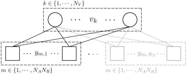
Figure 5: Factor graph of the linear system formulated for the estimation of $\mathbf{v}$.

Utilizing the soft-replicas and their MSEs, the factor nodes perform soft-interference cancellation (IC) on the received signal $y_{m,t}$ for each variable $v_{k}$, yielding the IC symbol

$$\bar{y}_{k:m,t}^{v}\!=\!y_{m,t}-\!\sum_{u=1}^{N_{U}}\!h_{m,u}x_{u,t}-\!\sum_{i\neq k}^{N_{V}}\!\Big{[}a_{m,i}\hat{v}_{i:m,t}\!\overbrace{\sum_{u=1}^{N_{U}}b_{i,u}x_{u,t}}^{\triangleq c_{i,t}}\!\Big{]}\!\!=\!v_{k}\big{(}a_{m,k}c_{k,t}\big{)}+\!\overbrace{\sum_{i\neq k}^{N_{V}}\!a_{m,i}(v_{i}\!-\!\hat{v}_{i:m,t})c_{i,t}\!+\!w_{m,t}}^{\text{\lx@glossaries@gls@link{acronym}{SGA}{\leavevmode scalar Gaussian approximation} (\lx@glossaries@gls@link{acronym}{SGA}{\leavevmode SGA})}},$$

(9)

where $x_{n,t}$ and $w_{m,t}$ are the ($n,t$)-th and ($m,t$)-th elements of $\mathbf{X}$ and $\mathbf{W}$, with $n\in\{1,\cdots,N_{U}\}$; and $c_{k,t}\triangleq\sum_{u=1}^{N_{U}}b_{k,u}x_{u,t}$ represents the aggregated incident signal at the $k$-th voxel from all UEs.

Next, by leveraging the central limit theorem (CLT), the sum of difference and noise terms are approximated as a complex Gaussian scalar, such that the PDF of the interference-cancelled symbols $\bar{y}_{k:m,t}^{v}$ can be modeled as

$$\mathbb{P}_{\bar{\mathsf{y}}^{\mathsf{v}}_{k:m,t}}(\bar{y}^{v}_{k:m,t}|v_{k})\propto\mathrm{exp}\Big{[}\!-\!\frac{|\bar{y}^{v}_{k:m,t}-v_{k}\big{(}a_{m,k}c_{k,t}\big{)}|^{2}}{\nu^{v}_{k:m,t}}\Big{]},$$ (10)

with the corresponding conditional variance $\nu^{v}_{k:m,t}$ given by

$$\nu^{v}_{k:m,t}=\mathbb{E}_{\mathsf{v}_{k}}[|\bar{y}_{k:m,t}^{v}-(a_{m,k}c_{k,t})v_{k}|^{2}]=\sum_{i\neq k}^{N_{V}}|a_{m,i}|^{2}|c_{i,t}|^{2}\psi^{v}_{i:m,t}+N_{0},\vspace{-1ex}$$ (11)

where $N_{0}\triangleq\mathbb{E}_{\mathsf{w}_{m,t}}[|w_{m,t}|^{2}]$ is the noise variance.

The conditional variances for all $v_{k}$ are computed by all factor nodes, and the message is sent to the corresponding variable nodes. Consequently, the $k$-th variable node obtains the $N_{A}N_{R}N_{T}$ conditional variances from all factor nodes, from which the extrinsic belief $\ell^{v}_{k}$ is computed. In GaBP, self-interference is suppressed by excluding the conditional PDF of $\bar{y}_{k:m,t}$ at the $k$-th variable node to yield $\ell^{v}_{k:m,t}$ with the PDF

$$\mathbb{P}_{\mathsf{l}^{\mathsf{v}}_{k:m,t}}(\ell^{v}_{k:m,t}|v_{k})=\!\!\!\!\prod_{p\neq m}^{N_{A}N_{R}}\!\prod_{q\neq t}^{N_{T}}\mathbb{P}_{\bar{\mathsf{y}}^{\mathsf{v}}_{k:m,t}}(\bar{y}^{v}_{k:p,q}|v_{k})\propto\mathrm{exp}\Bigg{[}-\frac{|v_{k}-\mu^{v}_{k:m,t}|^{2}}{\varPsi^{v}_{k:m,t}}\Bigg{]},\\$$ (12)

where the extrinsic mean $\mu^{v}_{k:m,t}$ and variance $\varPsi^{v}_{k:m,t}$ is respectively given by

$$\mu^{v}_{k:m,t}=\varPsi^{v}_{k:m,t}\cdot\Bigg{(}\sum_{p\neq m}^{N_{A}N_{R}}\!\!\sum_{q\neq t}^{N_{T}}\!\frac{\big{(}a_{p,k}c_{k,t}\big{)}^{*}\cdot\bar{y}^{v}_{k:p,q}}{\nu^{v}_{k:p,q}}\Bigg{)}~{}\text{and}~{}\varPsi^{v}_{k:m,t}=\Bigg{(}\sum_{p\neq m}^{N_{A}N_{R}}\!\!\sum_{q\neq t}^{N_{T}}\!\frac{|a_{p,k}|^{2}|c_{k,t}|^{2}}{\nu^{v}_{k:p,q}}\Bigg{)}^{\!-1}\!\!\!\!.$$ (13)

Finally, by following the Bayes rule, the updated posterior may be obtained by combining the PDF of the extrinsic belief and the prior distribution of $v_{k}$, from which the updated soft-replica is obtained as

$$\hat{v}_{k:m,t}=\dfrac{\mathbb{E}_{\mathsf{v}_{k}}\!\!\left[\mathbb{P}_{\mathsf{l}^{\mathsf{v}}_{k:m,t}}(\ell^{v}_{k:m,t}|v_{k})\cdot\mathbb{P}_{\mathsf{v}_{k}}(v_{k})\right]}{\int_{\mathsf{v_{k}}}\!\!\mathbb{P}_{\mathsf{l}^{\mathsf{v}}_{k:m,t}}(\ell^{v}_{k:m,t}|v_{k})\cdot\mathbb{P}_{\mathsf{v}_{k}}(v_{k})},$$ (14)

where the normalizing factor in the denominator is the integrated updated posterior over $\mathbb{C}$.

Similarly, the updated error variance of the soft-replica is obtained by evaluating

$$\psi^{v}_{k:m,t}=\dfrac{\mathrm{Var}_{\mathsf{v}_{k}}\!\!\left[\mathbb{P}_{\mathsf{l}_{k:m,t}^{\mathsf{v}}}(\ell^{v}_{k:m,t}|v_{k})\cdot\mathbb{P}_{\mathsf{v}_{k}}(v_{k})\right]}{\int_{\mathsf{v_{k}}}\!\!\mathbb{P}_{\mathsf{l}^{\mathsf{v}}_{k:m,t}}(\ell^{v}_{k:m,t}|v_{k})\cdot\mathbb{P}_{\mathsf{v}_{k}}(v_{k})}.$$ (15)

Given the information of the voxel coefficient distributions, i.e., binary coefficients with a discrete prior given by a Bernoulli distribution with occupancy probability $E_{v}\triangleq\mathbb{P}_{\mathsf{v_{k}}}(v_{k}=1)$, the soft-replica and its MSE can be efficiently obtained in closed-form, respectively given by

$$\hat{v}_{k:m,t}=\bigg{(}1+\dfrac{1-E_{v}}{E_{v}}\mathrm{exp}\Big{(}-\dfrac{|{\mu}^{v}_{k:m,t}|^{2}-|1-{\mu}^{v}_{k:m,t}|^{2}}{\varPsi^{v}_{k:m,t}}\Big{)}\bigg{)}^{\!-1}\!\!\!\!,$$ (16)

$$\psi^{v}_{k:m,t}=(\hat{v}_{k:m,t})^{2}+E_{v}-2E_{v}\hat{v}_{k:m,t}.$$ (17)

The updated soft-replica and the MSE of each variable node are then transmitted back to all factor nodes for the next iteration of the GaBP MP algorithm. After a given number of GaBP iterations to refine the soft-estimates, a belief consensus is taken at each variable node across the soft-replicas to obtain a single estimate $\tilde{\mathbf{v}}$ by

$$\mathbb{P}_{\tilde{\mathsf{l}}^{\mathsf{v}}_{k}}(\tilde{\ell}^{v}_{k}|v_{k})=\!\!\!\!\prod_{p=1}^{N_{A}N_{R}}\!\prod_{q=1}^{N_{T}}\mathbb{P}_{\bar{\mathsf{y}}^{\mathsf{v}}_{k:m,t}}(\bar{y}^{v}_{k:p,q}|v_{k})\propto\mathrm{exp}\left[-\frac{|v_{k}-\tilde{\mu}^{v}_{k}|^{2}}{\tilde{\varPsi}^{v}_{k}}\right],\\$$ (18)

with consensus mean $\tilde{\mu}^{v}_{k}$ and variance $\tilde{\varPsi}^{v}_{k}$ expressed as

$$\tilde{\mu}^{v}_{k}=\tilde{\varPsi}^{v}_{k}\cdot\Bigg{(}\sum_{p=1}^{N_{A}N_{R}}\!\sum_{q=1}^{N_{T}}\frac{\big{(}a_{p,k}c_{k,t}\big{)}^{*}\cdot\bar{y}^{v}_{k:p,q}}{\nu^{v}_{k:p,q}}\Bigg{)}\quad\text{and}\quad\tilde{\varPsi}^{v}_{k}=\Bigg{(}\sum_{p=1}^{N_{A}N_{R}}\!\sum_{q=1}^{N_{T}}\frac{|a_{p,k}|^{2}|c_{k,t}|^{2}}{\nu^{v}_{k:p,q}}\Bigg{)}^{\!\!\!-1}\!\!\!\!,$$ (19)

which is consequently used to yield the final estimate by

$$\tilde{v}_{k}=\dfrac{\mathbb{E}_{{\mathsf{v}}_{k}}\!\Big{[}\mathbb{P}_{\tilde{\mathsf{l}}^{\mathsf{v}}_{k}}(\tilde{\ell}^{v}_{k}|v_{k})\cdot\mathbb{P}_{{\mathsf{v}}_{k}}(v_{k})\Big{]}}{\int_{{v}_{k}}\!\!\mathbb{P}_{\tilde{\mathsf{l}}^{\mathsf{v}}_{k}}(\tilde{\ell}^{v}_{k}|v_{k})\cdot\mathbb{P}_{{\mathsf{v}}_{k}}(v_{k})}.$$ (20)

The above MP equations (8) to (20) fully describe the linear GaBP module to estimate the voxel environment $\mathbf{v}$, which is summarized as a pseudocode in Algorithm 1. It is important to note that the signal matrix $\mathbf{X}$ is assumed given – i.e., $\mathbf{X}$ is not estimated by Algorithm 1 – and therefore is kept constant throughout the iterations, as seen by the pre-computation of the effective signals $c_{k,t}$. The complementary block dedicated to the estimation of $\mathbf{X}$ given $\mathbf{v}$ will be described subsequently, leading to an alternate approach as previously mentioned. The algorithm also contains a damping update mechanism [69] using a damping factor $\eta\in[0,1]$ to prevent early convergence to a local optimum.

1: Inputs: Received signal matrix $\mathbf{Y}$, channel matrices $\mathbf{H}$, $\mathbf{A}$, and $\mathbf{B}$, transmit signal matrix $\mathbf{X}$, noise variance $N_{0}$, prior distribution of voxels $\mathbb{P}_{\mathsf{v}_{k}}(v_{k})$, and pre-computation of $\mathbf{C}=\mathbf{B}\mathbf{X}$.

2: Outputs: Estimated voxel environment vector $\tilde{\mathbf{v}}$.

3:

4:Initialize the soft-replica at all variable nodes as $\hat{v}_{k:m,t}=\mathbb{E}_{\mathsf{v}_{k}}[v_{k}]$; $\triangleright$ $\forall k,m,t$

5:Initialize the MSEs at all variable nodes $\psi^{v}_{k:m,t}$ via (8); $\triangleright$ $\forall k,m,t$

6: Until termination criteria is satisfied$\color[rgb]{0,0,0}^{*}$ do

7:   Compute the soft-IC performed received signal $\bar{y}_{k:m,t}^{v}$ via (9); $\triangleright$ $\forall k,m,t$

8:   Compute the conditional variance ${\nu}^{v}_{k:m,t}$ via (11); $\triangleright$ $\forall k,m,t$

9:   Compute the extrinsic mean ${\mu}^{v}_{k:m,t}$ and variance ${\varPsi}^{v}_{k:m,t}$ via (13); $\triangleright$ $\forall k,m,t$

10:   Compute the new soft-replica $\hat{v}_{k:m,t}$ and the MSE $\psi^{v}_{k:m,t}$ via (14)-(15); $\triangleright$ $\forall k,m,t$

11:   Update the soft-replica $\hat{v}_{k:m,t}$ and the MSE $\psi^{v}_{k:m,t}$ via damping [69]; $\triangleright$ $\forall k,m,t$

12:end

13:Compute the consensus mean $\tilde{\mu}^{v}_{k}$ and variance $\tilde{\varPsi}^{v}_{k}$ via (19); $\triangleright$ $\forall k$

14:Compute the final soft-estimate $\tilde{v}_{k}$ via (20); $\triangleright$ $\forall k$

Algorithm 1 : Linear GaBP Estimator for Environment (Voxel Coefficients) Vector $\mathbf{v}$

${}^{*}\!$ The termination criteria can be set as the maximum number of MP iterations or the convergence threshold of the soft-replicas,
depending on the desired accuracy or complexity. A discussion o appropriate values are provided in Section IV-C.

III-A2 Linear GaBP for Signal Matrix $\mathbf{X}$

 

In order to derive the linear GaBP module to estimate the signal matrix $\mathbf{X}$ given $\mathbf{v}$, the system model in (6) is first reduced to the one in (4), with the effective channel $\mathbf{G}\triangleq\big{(}\mathbf{H}+\mathbf{A}{\mathrm{diag}}\!\left({\mathbf{v}}\right)\!\mathbf{B}\big{)}$, with the corresponding factor graph as illustrated in Fig. 6, where each element $x_{n,t}$ of the unknown signal matrix $\mathbf{X}$ with $n\in\{1,\cdots,N_{U}\}$, is the variable node (circular nodes).

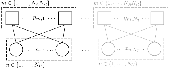
Figure 6: The separated factor graphs of the linear system for $\mathbf{X}$.

Notice that in this case, since the variable $\mathbf{X}$ is two-dimensional, the linear system results in a factor graph that is separated into “pages”, such that the variable nodes and factor nodes corresponding to different $t\in\{1,\cdot,N_{T}\}$ are independent and that the messages are only exchanged by nodes with the same time index $t$. Other than this separation of factor graphs, the derivation of the MP rules is similar to that of Algorithm 1.

The soft-replica of the transmit signal matrix element $x_{n,t}$ to the $(m,t$)-th factor node is denoted by $\hat{x}_{m,t:n,t}$, with the corresponding MSE given by

$$\psi^{x}_{m,t:n,t}=\mathbb{E}_{\mathsf{x}_{n,t}}[|x_{n,t}-\hat{x}_{m,t:n,t}|^{2}].\vspace{-0.5ex}$$ (21)

The soft-replica and the MSE are used in the soft-IC of the received signals for $x_{n,t}$, following

$$\bar{y}^{x}_{n,t:m,t}=y_{m,t}-\sum^{N_{U}}_{u\neq n}g_{m,u}\hat{x}_{u,t:m,t}=g_{m,n}x_{n,t}+\sum^{N_{U}}_{u\neq n}g_{m,u}(x_{u,t}-\hat{x}_{u,t:m,t})+w_{m,t},$$ (22)

with the conditional PDF described by

$$\mathbb{P}_{\bar{\mathsf{y}}^{\mathsf{x}}_{n,t:m,t}}(\bar{y}^{x}_{n,t:m,t}|x_{n,t})\propto\mathrm{exp}\left[-\frac{|\bar{y}^{x}_{n,t:m,t}-g_{m,n}x_{n,t}|^{2}}{\nu^{x}_{n,t:m,t}}\right],$$ (23)

and the conditional variance $\nu^{x}_{n,t:m,t}$ is given by

$$\nu^{x}_{n,t:m,t}=\mathbb{E}_{\mathsf{x}_{n,t}}[|\bar{y}^{x}_{n,t:m,t}-g_{m,n}x_{n,t}|^{2}]=\sum_{u\neq n}^{N_{U}}|g_{m,u}|^{2}\psi^{x}_{u,t:m,t}+N_{0}.\vspace{-1ex}$$ (24)

The conditional PDFs are combined with self-interference cancellation at the variable nodes to yield the extrinsic beliefs $\ell^{x}_{n,t:m,t}$ following

$$\mathbb{P}_{\mathsf{l}^{\mathsf{x}}_{n,t:m,t}}(\ell^{x}_{n,t:m,t}|x_{n,t})=\prod_{p\neq m}^{N_{A}N_{R}}\mathbb{P}_{\bar{\mathsf{y}}^{\mathsf{x}}_{n,t:p,t}}(\bar{y}^{x}_{n,t:p,t}|x_{n,t})\propto\mathrm{exp}\left[-\frac{|x_{n,t}-\mu^{x}_{n,t:m,t}|^{2}}{\varPsi^{x}_{n,t:m,t}}\right],\\$$ (25)

with the extrinsic mean $\mu^{x}_{n,t:m,t}$ and variance $\varPsi^{x}_{n,t:m,t}$ respectively given by

$$\mu^{x}_{n,t:m,t}=\varPsi^{x}_{n,t:m,t}\cdot\Bigg{(}\sum_{p\neq m}^{N_{A}N_{R}}\frac{(g_{p,n})^{*}\!\cdot\bar{y}^{x}_{n,t:p,t}}{\nu^{x}_{n,t:p,t}}\Bigg{)}\quad\text{and}\quad\varPsi^{x}_{n,t:m,t}=\Bigg{(}\sum_{p\neq m}^{N_{A}N_{R}}\frac{|g_{p,n}|^{2}}{\nu^{x}_{n,t:p,t}}\Bigg{)}^{\!-1}\!\!\!\!.$$ (26)

In turn, since the symbols have a uniformly discrete prior from the symbol constellation $\mathcal{X}$, with the symbol probability $\mathbb{P}_{\mathsf{x}}(x)=1/|\mathcal{X}|$, their soft-replicas and MSEs are obtained by

$$\hat{x}_{n,t:m,t}=\dfrac{\sum_{x\in\mathcal{X}}x\cdot\mathbb{P}_{\mathsf{l}^{\mathsf{x}}_{n,t:m,t}}(\ell^{x}_{n,t:m,t}|x)\cdot\mathbb{P}_{\mathsf{x}}(x)}{\sum_{x\in\mathcal{X}}\mathbb{P}_{\mathsf{l}^{\mathsf{x}}_{n,t:m,t}}(\ell^{x}_{n,t:m,t}|x)\cdot\mathbb{P}_{\mathsf{x}}(x)}\;,$$ (27)

$$\psi^{x}_{n,t:m,t}=\dfrac{\sum_{x\in\mathcal{X}}x^{2}\cdot\mathbb{P}_{\mathsf{l}^{\mathsf{x}}_{n,t:m,t}}(\ell^{x}_{n,t:m,t}|x)\cdot\mathbb{P}_{\mathsf{x}}(x)}{\sum_{x\in\mathcal{X}}\mathbb{P}_{\mathsf{l}^{\mathsf{x}}_{n,t:m,t}}(\ell^{x}_{n,t:m,t}|x)\cdot\mathbb{P}_{\mathsf{x}}(x)}-(\hat{x}_{n,t:m,t})^{2}.$$ (28)

For the particular case of $M$-ary quadrature amplitude modulation ($M$-QAM) with $M=4$, the soft-replica and MSE computations reduce to efficient closed-form expressions given by

$$\hat{x}_{n,t:m,t}=\sqrt{\frac{E_{\mathcal{X}}}{{2}}}\cdot\left(\mathrm{tanh}\left[\sqrt{\frac{2}{E_{\mathcal{X}}}}\cdot\frac{\Re{\{\mu^{x}_{n,t:m,t}\}}}{\varPsi^{x}_{n,t:m,t}}\right]+j\mathrm{tanh}\left[\sqrt{\frac{2}{E_{\mathcal{X}}}}\cdot\frac{\Im{\{\mu^{x}_{n,t:m,t}\}}}{\varPsi^{x}_{n,t:m,t}}\right]\right),$$ (29)

$$\psi^{x}_{n,t:m,t}=E_{\mathcal{X}}-|\hat{x}_{n,t:m,t}|^{2},\vspace{-1ex}$$ (30)

where $E_{\mathcal{X}}\triangleq\mathbb{E}_{x}[|x|^{2}]$ denotes the average symbol power of the constellation $\mathcal{X}$, and $\mathrm{tanh}(\cdot)$ denotes the trigonometric hyperbolic tangent function.

Finally, the consensus PDF, which is taken after the iterations is given by

$$\mathbb{P}_{\tilde{\mathsf{l}}^{\mathsf{x}}_{n,t}}(\tilde{\ell}^{x}_{n,t}|x_{n,t})=\prod_{p=1}^{N_{A}N_{R}}\mathbb{P}_{\bar{\mathsf{y}}^{\mathsf{x}}_{n,t:m,t}}(\bar{y}^{x}_{n,t:p,t}|x_{n,t})\propto\mathrm{exp}\left[-\frac{|x_{n,t}-\tilde{\mu}^{x}_{n,t}|^{2}}{\tilde{\varPsi}^{x}_{n,t}}\right],\\$$ (31)

with the consensus mean $\tilde{\mu}^{x}_{n,t}$ and variance $\tilde{\varPsi}^{x}_{n,t}$ expressed as

$$\tilde{\mu}^{x}_{n,t}=\varPsi^{x}_{n,t}\cdot\Bigg{(}\sum_{p=1}^{N_{A}N_{R}}\frac{(g_{p,n})^{*}\cdot\bar{y}^{x}_{n,t:p,t}}{\nu^{x}_{n,t:p,t}}\Bigg{)}\quad\text{and}\quad\tilde{\varPsi}^{x}_{n,t}=\Bigg{(}\sum_{p=1}^{N_{A}N_{R}}\frac{|g_{p,n}|^{2}}{\nu^{x}_{n,t:p,t}}\Bigg{)}^{\!\!\!-1}\!\!\!\!\!,$$ (32)

yielding the final soft estimate

$$\tilde{x}_{n,t}=\dfrac{\sum_{x\in\mathcal{X}}x\cdot\mathbb{P}_{\tilde{\mathsf{l}}^{\mathsf{x}}_{n,t}}(\tilde{\ell}^{x}_{n,t}|x_{n,t})\cdot\mathbb{P}_{{\mathsf{x}}_{n,t}}(x_{n,t})}{\sum_{x\in\mathcal{X}}\mathbb{P}_{\tilde{\mathsf{l}}^{\mathsf{x}}_{n,t}}(\tilde{\ell}^{x}_{n,t}|x_{n,t})\cdot\mathbb{P}_{{\mathsf{x}}_{n,t}}(x_{n,t})}.$$ (33)

Equations (21) to (33), collected in the form of a pseudocode in Algorithm 2, fully describe the linear GaBP module for the estimation of the signal matrix $\mathbf{X}$ given the environment vector $\mathbf{v}$, which together with the previously described module for the estimation of $\mathbf{v}$ given $\mathbf{X}$, completes the proposed AL-ISAC scheme. All that remains is to describe the alternating procedure to estimate both unknown variables, which is addressed in the sequel.

1: Inputs: Received signal matrix $\mathbf{Y}$, channel matrices $\mathbf{H}$, $\mathbf{A}$, and $\mathbf{B}$, environment vector $\mathbf{v}$,   noise variance $N_{0}$, and prior distribution of transmit symbols $\mathbb{P}_{\mathsf{x}_{n,t}}(x_{n,t})$.

2: Outputs: Estimated transmit signal matrix $\tilde{\mathbf{X}}$.

3:

4:Compute the effective channel matrix $\mathbf{G}\triangleq\mathbf{H}+\mathbf{A}{\mathrm{diag}}\!\left({\mathbf{v}}\right)\!\mathbf{B}$;

5:Initialize the soft-replica at all variable nodes as $\hat{x}_{n,t:m,t}=\mathbb{E}_{\mathsf{x}_{n,t}}[x_{n,t}];$ $\triangleright$ $\forall m,n,t$

6:Initialize the MSE at all variable nodes as $\psi^{x}_{n,t:m,t}$ via (21); $\triangleright$ $\forall m,n,t$

7: Until termination criteria is satisfied$\color[rgb]{0,0,0}^{*}$ do

8:   Compute the soft-IC performed received signal $\bar{y}_{n,t:m,t}^{x}$ via (22); $\triangleright$ $\forall m,n,t$

9:   Compute the conditional variance ${\nu}^{x}_{n,t:m,t}$ via (24); $\triangleright$ $\forall m,n,t$

10:   Compute the extrinsic mean ${\mu}^{x}_{n,t:m,t}$ and variance ${\varPsi}^{x}_{n,t:m,t}$ via (26); $\triangleright$ $\forall m,n,t$

11:   Compute the new soft-replica $\hat{x}_{n,t:m,t}$ and the MSE $\psi^{x}_{n,t:m,t}$ via (27) and (28); $\triangleright$ $\forall m,n,t$

12:   Update the soft-replica $\hat{x}_{n,t:m,t}$ and the MSE $\psi^{x}_{n,t:m,t}$ via damping [69]; $\triangleright$ $\forall m,n,t$

13: end

14:Compute the consensus mean $\tilde{\mu}^{x}_{n,t}$ and variance $\tilde{\varPsi}^{x}_{n,t}$ via (32); $\triangleright$ $\forall n,t$

15:Compute the final soft-estimate $\tilde{x}_{n,t}$ via (33); $\triangleright$ $\forall n,t$

16:Project $\tilde{x}_{n,t}$ to the symbol constellation $\mathcal{X}$; $\triangleright$ $\forall n,t$

17:Output projected $\tilde{x}_{n,t}$ as final hard estimate; $\triangleright$ $\forall n,t$

Algorithm 2 : Linear GaBP Estimator for Signal Matrix $\mathbf{X}$

${}^{*}\!$ The termination criteria can be set in accordance to Section IV-C and as described in Algorithm 1.

III-A3 Combined Alternating Modular Structure

 

With the two estimation modules given by Algorithm 1 and Algorithm 2, either of the two variables $\mathbf{v}$ or $\mathbf{X}$ may be estimated, assuming full information of the other variable. However, the very inherent problem of ISAC in equation (6), is that neither of the variables are fully known such that the linear modules may not be directly applied for estimation.

To address the problem, the proposed AL-ISAC algorithm successively applies the two linear GaBP modules to estimate the two sets of variables. To enable this, the received signal is separated into the blocks corresponding to the pilot phase and the data phase, as

$$\mathbf{Y}_{P} =\big{(}\mathbf{H}+\mathbf{A}{\mathrm{diag}}\!\left({\mathbf{v}}\right)\!\mathbf{B}\big{)}\mathbf{X}_{P}+\mathbf{W}_{P}\in\mathbb{C}^{N_{A}N_{R}\times N_{P}},$$ (34a)

$$\mathbf{Y}_{D} =\big{(}\mathbf{H}+\mathbf{A}{\mathrm{diag}}\!\left({\mathbf{v}}\right)\!\mathbf{B}\big{)}\mathbf{X}_{D}+\mathbf{W}_{D}\in\mathbb{C}^{N_{A}N_{R}\times N_{D}},$$ (34b)

where $\mathbf{Y}\triangleq[\mathbf{Y}_{P}\;\mathbf{Y}_{D}]$ and $\mathbf{W}\triangleq[\mathbf{W}_{P}\;\mathbf{W}_{D}]$, as defined with $\mathbf{X}=[\mathbf{X}_{P}\;\mathbf{X}_{D}]$.

First, by using only the pilot phase of the system (34a), Algorithm 1 is applied to estimate the initial environment vector $\tilde{\mathbf{v}}_{init}$ with the pilot block $\mathbf{X}_{P}$ as known input signal matrix.

Next, by using the data phase of the system (34b), Algorithm 2 is applied to estimate the unknown data block $\tilde{\mathbf{X}}_{D}$ using the initial environment estimate $\tilde{\mathbf{v}}_{init}$ as the known input environment vector. Finally, the environment vector is obtained by using Algorithm 2 again, but with the initial environment estimate $\tilde{\mathbf{v}}_{init}$ as the initialization value of the soft-replicas at all factor nodes, and $[\mathbf{X}_{P}\;\tilde{\mathbf{X}}_{D}]$ as the input transmit signal matrix. The described AL-ISAC algorithm is illustrated in a schematic form in Fig. 7, and summarized as pseudocode in Algorithm 3.

1: Inputs: Received signal matrix $\mathbf{Y}$, channel matrices $\mathbf{H}$, $\mathbf{A}$, and $\mathbf{B}$, pilot matrix $\mathbf{X}_{P}$, noise variance $N_{0}$, prior distribution of environment and transmit symbols $\mathbb{P}_{\mathsf{v}_{k}}(v_{k})$ and $\mathbb{P}_{\mathsf{x}_{n,t}}(x_{n,t})$.

2: Outputs: Estimated environment vector $\tilde{\mathbf{v}}$ and estimated data signal matrix $\tilde{\mathbf{X}}_{D}$.

3:

4: Using only the block corresponding to the pilot sequence, i.e., $t=\{1,\cdots,N_{P}\}$:

5:Estimate initial environment $\tilde{\mathbf{v}}_{init}$ via Algorithm 1, using pilot $\mathbf{X}_{P}$ as known signal input.

6: Using only the block corresponding to the data sequence, i.e., $t=\{N_{P}+1,\cdots,N_{P}+N_{D}\}$:

7:Estimate data signal $\tilde{\mathbf{X}}_{D}$ via Algorithm 2, using $\tilde{\mathbf{v}}_{init}$ as known environment input.

8: Using the entire time block, i.e., $t=\{1,\cdots,N_{P}+N_{D}\}$:

9:Estimate $\tilde{\mathbf{v}}$ via Algorithm 1, using $[\mathbf{X}_{P},\!{\color[rgb]{0,0,0}~{}\tilde{\mathbf{X}}_{D}}]$ as the signal input, and $\tilde{\mathbf{v}}_{init}$ as initialization.

10:Output $\tilde{\mathbf{v}}$ as the estimated environment vector, and ${\color[rgb]{0,0,0}\tilde{\mathbf{X}}_{D}}$ as estimated data signal matrix.

Algorithm 3 : Proposed Alternating Linear ISAC (AL-ISAC)Algorithm${}^{\dagger}\!$

${}^{\dagger}\!\!$ Although our simulations indicate that a single iteration (as shown in Fig. 7) is sufficient, the linear GaBP modules in steps 2
and 3 can be iterated multiple times, with feedback at modular level and possibly adaptive MP denoising between feedback
loops. These, and other potential improvements remain open points for a follow up work.

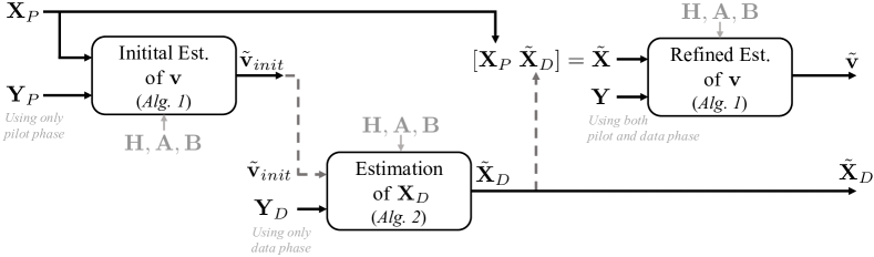
Figure 7: A schematic diagram of the proposed AL-ISAC algorithm (Algorithm 3).

Despite having a potential complexity advantage, especially for scenarios with large numbers of UEs, as shown later in Subsection IV-A, the alternating approach of the AL-ISAC algorithm has the drawback of causing a heavy dependence on the length of the pilot sequence $\mathbf{X}_{P}$, which as shall be shown in Section IV, affects the performance of both environment and data signal estimation, in addition to the obvious trade-off with the total communication throughput. Aiming to circumvent this deficiency, in the next subsection we propose another ISAC method in which both $\mathbf{v}$ and $\mathbf{X}_{D}$ are estimated simultaneously via a bilinear inference method.

III-B Proposed Bilinear ISAC Algorithm (Bi-ISAC)

In this section, we develop a new ISAC algorithm in which the sensing and communication variables $\mathbf{v}$ and $\mathbf{X}_{D}$ are estimated in parallel, by using a bilinear message passing technique which incorporates the uncertainty of both estimates at each iteration, thus requiring only a single estimation module to acquire both variables, as illustrated in Fig. 8.

We start by observing that the unique asymmetric bilinear relationship of $\mathbf{v}$ and $\mathbf{X}_{D}$, as per equation (7), prevents the application of recently discovered bilinear estimators, such as the bilinear generalized approximate message passing (BiGAMP) [63], which operates only on symmetric systems described by equations in the form $\mathbf{Y}=\mathbf{V}\mathbf{X}+\mathbf{W}$ for the joint estimation of the unknowns $\mathbf{V}$ and $\mathbf{X}$; or the parametric BiGAMP [66, 67], which works on systems with the structure $\mathbf{Y}=\sum_{k}\!v_{k}\mathbf{A}_{k}\mathbf{X}+\mathbf{W}$ to jointly estimate $v_{k}$ and $\mathbf{X}$ with known $\mathbf{A}_{k}$.

In contrast to these two examples, the problem dealt with here is, as described by equation (6), in neither of the aforementioned forms, nor can it be transformed to fit general bilinear forms, which implies that new, purpose-built bilinear Gaussian belief propagation (BiGaBP) [64, 65, 68] MP rules must be derived for its solution. Therefore, the BiGaBP message passing is performed on a tripartite factor graph as illustrated in Fig. 9, where the factor nodes (square

 

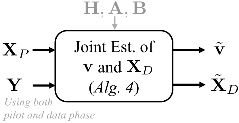
Figure 8: A schematic diagram of the proposed Bi-ISAC algorithm (Algorithm 4).

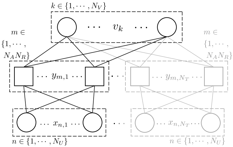
Figure 9: The tripartite factor graph of the bilinear system.

nodes) are the received symbols, and the two sets of variable nodes (circular nodes) corresponds to the environment vector $\mathbf{v}$ and the signal matrix $\mathbf{X}$, respectively. An important distinction is made between the two types of variable nodes, which is that a data variable node receives messages only from $N_{A}N_{R}$ factor nodes corresponding to the same time instance $t$, while an environment variable node receives messages from all $N_{A}N_{R}N_{T}$ factor nodes.

We highlight the higher complexity of the factor graph in Fig. 9 compared to those of linear GaBP schemes shown in Figs. 5 and 6, due to the asymmetric and embedded system structure of equation (6) in relation to both variables together, as opposed to those of linear systems where one variable is considered at a time. Other than that, the messages transferred over the graph edges are the same information as in the linear GaBP in Section III-A, i.e., the soft-replicas, MSEs, and conditional PDFs of the variables of interest. However, since neither of the latter is known, except as soft-replicas, the corresponding calculation of the messages must incorporate the uncertainties in both variables, in the form of the respective MSEs.

In light of the above, similarly to Section III-A, the exchanged messages are constructed on the basis of soft-replicas of the variables. Since the entries in $\mathbf{X}$ corresponding to $t\in\{1,\cdots,N_{P}\}$ are pilot symbols $\mathbf{X}_{P}$, the corresponding soft-replicas are set to their known values, i.e., $\hat{x}_{n,t:m,t}=(x_{p})_{n,t}~{}\forall t\in\{1,\cdots,N_{P}\}$, with the corresponding MSE values set to $0$. The remaining soft-replicas and MSEs for $t\in\{N_{P}+1,\cdots,N_{T}\}$ are as given in equations (8) and (21).

The complete description of the proposed bilinear ISAC (Bi-ISAC) algorithm is summarized in the form of a pseudocode in Algorithm 4, and the corresponding equations of the message passing rules are elaborated in the following.

1: Inputs: Received signal matrix $\mathbf{Y}$, channel matrices $\mathbf{H}$, $\mathbf{A}$, and $\mathbf{B}$, pilot matrix $\mathbf{X}_{P}$, noise variance $N_{0}$, prior distribution of environment and transmit symbols $\mathbb{P}_{\mathsf{v}_{k}}(v_{k})$ and $\mathbb{P}_{\mathsf{x}_{n,t}}(x_{n,t})$.

2: Outputs: Estimated environment vector $\tilde{\mathbf{v}}$ and estimated data signal matrix $\tilde{\mathbf{X}}_{D}$.

3:

4: For data variable nodes corresponding to the pilot block, i.e., for $t\in\{1,\cdots,N_{P}\}$,

5:Initialize the soft-replicas as pilots by $\hat{x}_{n,t:m,t}=(x_{p})_{n,t};$ $\triangleright$ $\forall m,n$

6:Initialize the MSEs $\psi^{x}_{n,t:m,t}$ to $0$; $\triangleright$ $\forall m,n$

7: For data variable nodes corresponding to the data block, i.e., for $t\in\{N_{P}+1,\cdots,N_{T}\}$,

8:Initialize the soft-replicas as $\hat{x}_{n,t:m,t}=\mathbb{E}_{\mathsf{x}_{n,t}}[x_{n,t}];$ $\triangleright$ $\forall m,n$

9:Initialize the MSEs $\psi^{x}_{n,t:m,t}$ via (21); $\triangleright$ $\forall m,n$

10: For all environment variable nodes, i.e., for $t\in\{1,\cdots,N_{T}\}$,

11:Initialize the environment soft-replicas as $\hat{v}_{k:m,t}=\mathbb{E}_{\mathsf{v}_{k}}[v_{k}]$; $\triangleright$ $\forall m,k$

12:Initialize the MSEs $\psi^{v}_{k:m,t}$ via (8); $\triangleright$ $\forall m,k$

13: Until termination criteria is satisfied^∗ do

14:   Compute the soft-IC signals $\bar{y}_{k:m,t}^{v}$ and $\bar{y}_{n,t:m,t}^{x}$ via (35); $\triangleright$ $\forall m,n,k,t$

15:   Compute the conditional variances ${\nu}^{v}_{k:m,t}$ and ${\nu}^{x}_{n,t:m,t}$ via (38); $\triangleright$ $\forall m,n,k,t$

16:   Compute the extrinsic mean ${\mu}^{v}_{k:m,t}$ and variance ${\varPsi}^{v}_{k:m,t}$ via (41); $\triangleright$ $\forall m,n,k,t$

17:   Compute the extrinsic mean ${\mu}^{x}_{n,t:m,t}$ and variance ${\varPsi}^{x}_{n,t:m,t}$ via (42); $\triangleright$ $\forall m,n,k,t$

18:   Compute the new soft-replicas $\hat{v}_{k:m,t}$ and $\hat{x}_{n,t:m,t}$ via (14) and (27); $\triangleright$ $\forall m,n,k,t$

19:   Compute the new MSEs $\psi^{v}_{k:m,t}$ and $\psi^{x}_{n,t:m,t}$ via (15) and (28); $\triangleright$ $\forall m,n,k,t$

20:   Update all soft-replicas and MSEs via damping [69]; $\triangleright$ $\forall m,n,k,t$

21: end

22:Compute the consensus PDFs with $\tilde{\mu}^{v}_{k}$ and $\tilde{\varPsi}^{v}_{k}$ via (19), and $\tilde{\mu}^{x}_{n,t}$ and $\tilde{\varPsi}^{x}_{n,t}$ via (32); $\triangleright$ $\forall n,k,t$

23:Compute the final soft-estimates $\tilde{v}_{k}$ and $\tilde{x}_{n,t}$ via (20) and (33); $\triangleright$ $\forall n,k,t$

24:Output $\tilde{v}_{k}$ as final estimate; $\triangleright$ $\forall k$

25:Project $\tilde{x}_{n,t}$ to the symbol constellation $\mathcal{X}$; $\triangleright$ $\forall n,~{}\forall t\in\{N_{P}+1,\cdots,N_{T}\}$

26:Output projected $\tilde{x}_{n,t}$ as final estimate; $\triangleright$ $\forall n,~{}\forall t\in\{N_{P}+1,\cdots,N_{T}\}$

Algorithm 4 : Bilinear GaBP Estimator for Environment Vector $\mathbf{v}$ and Data Matrix $\mathbf{X}_{D}$

${}^{*}\!$ The termination criteria can be set in accordance to Section IV-C and as described in Algorithm 1.

In hand of the soft-replicas and their MSEs, the factor nodes perform soft-IC for each variable $v_{k}$ and $x_{n,t}$ by following

 

$$\bar{y}_{k:m,t}=y_{m,t}-\sum_{u}^{N_{U}}\Big{(}h_{m,u}+\sum_{i\neq k}^{N_{V}}a_{m,i}\hat{v}_{i:m,t}b_{i,u}\Big{)}\hat{x}_{u,t:m,t}$$

$$={v_{k}\Big{(}\!a_{m,k}\!\sum_{u}^{N_{U}}b_{k,u}x_{u,t}\!\Big{)}}\!+\!\!\sum_{u}^{N_{U}}h_{m,u}(x_{u,t}\!-\!\hat{x}_{u,t:m,t})\!+\!\!\sum_{u}^{N_{U}}\!\sum_{i\neq k}^{N_{V}}\!a_{m,i}b_{i,u}\left(v_{i}x_{u,t}\!-\!\hat{v}_{i:m,t}\hat{x}_{u,t:m,t}\right)\!+\!w_{m,t},$$

$$\bar{y}_{n,t:m,t}=y_{m,t}-\sum_{u\neq n}^{N_{U}}\Big{(}h_{m,u}+\sum_{i}^{N_{V}}a_{m,i}\hat{v}_{i:m,t}b_{i,u}\Big{)}\hat{x}_{u,t:m,t}$$

$$=\!x_{n,t}\Big{(}\!h_{m,n}\!+\!\!\sum_{i}^{N_{V}}a_{m,i}v_{i}b_{i,n}\!\Big{)}\!\!+\!\!\!\sum_{u\neq n}^{N_{U}}h_{m,u}(x_{u,t}\!-\!\hat{x}_{u,t:m,t})\!+\!\!\sum_{u\neq n}^{N_{U}}\!\sum_{i}^{N_{V}}\!a_{m,i}b_{i,u}\!\left(v_{i}x_{u,t}\!-\!\hat{v}_{i:m,t}\hat{x}_{u,t:m,t}\right)\!+\!w_{m,t},$$

where the soft-IC for the data variables given in (35) is only performed for unknown variable nodes with indices $t\in\{N_{P}+1,\cdots,N_{T}\}$.

Following the soft-IC, the respective conditional PDFs are become

$$\mathbb{P}_{\bar{\mathsf{y}}^{\mathsf{v}}_{k:m,t}}(\bar{y}^{v}_{k:m,t}|v_{k})\propto\mathrm{exp}\Big{[}\!-\!\frac{|\bar{y}^{v}_{k:m,t}-\big{(}a_{m,k}\sum_{u=1}^{N_{U}}b_{k,u}\!\cdot\!\hat{x}_{u,t:m,t}\big{)}v_{k}|^{2}}{\nu^{v}_{k:m,t}}\;\Big{]},$$ (36)

$$\mathbb{P}_{\bar{\mathsf{y}}^{\mathsf{x}}_{n,t:m,t}}(\bar{y}^{x}_{n,t:m,t}|x_{n,t})\propto\mathrm{exp}\Big{[}\!-\!\frac{|\bar{y}^{x}_{n,t:m,t}-\big{(}h_{m,n}+\sum_{i=1}^{N_{V}}a_{m,i}\!\cdot\!\hat{v}_{i:m,t}\!\cdot\!b_{i,n}\big{)}x_{n,t}|^{2}}{\nu^{x}_{n,t:m,t}}\;\Big{]},$$ (37)

with the respective conditional variances $\nu^{v}_{k:m,t}$ and $\nu^{x}_{n,t:m,t}$ given by

$${\nu^{v}_{k:m,t}} =\mathbb{E}_{\{\mathsf{v_{k}},\mathsf{x_{n,t}}\}}\Big{[}|\bar{y}^{v}_{k:m,t}-\big{(}a_{m,k}\sum_{u}^{N_{U}}b_{k,u}\!\cdot\!\hat{x}_{u,t:m,t}\big{)}v_{k}|^{2}\Big{]}$$ (38a)

$$=E_{v}\!\cdot\!|a_{m,k}|^{2}\sum_{u}^{N_{U}}|b_{k,u}|^{2}\psi^{x}_{u,t:m,t}+\sum_{u}^{N_{U}}|h_{m,u}|^{2}\psi^{x}_{u,t:m,t}$$

$$~{}~{}~{}+\sum_{u}^{N_{U}}\sum_{i\neq k}^{N_{V}}|a_{m,i}|^{2}\Big{(}\psi^{v}_{i:m,t}|\hat{x}_{u,t:m,t}|^{2}+\psi^{x}_{u,t:m,t}(|\hat{v}_{i:m,t}|^{2}+\psi^{v}_{i:m,t})\Big{)}|b_{i,u}|^{2}+N_{0},$$

$${\nu^{x}_{n,t:m,t}} =\mathbb{E}_{\{\mathsf{v_{k}},\mathsf{x_{n,t}}\}}\Big{[}|\bar{y}^{x}_{n,t:m,t}-\big{(}h_{m,n}+\sum_{i}^{N_{V}}a_{m,i}\!\cdot\!\hat{v}_{i:m,t}\!\cdot\!b_{i,n}\big{)}x_{n,t}|^{2}\Big{]}$$ (38b)

$$=E_{\mathcal{X}}\cdot\!\sum_{i}^{N_{V}}(|a_{m,i}|^{2}\psi^{v}_{i:m,t}|b_{i,n}|^{2})+\sum_{u\neq n}^{N_{U}}(|h_{m,u}|^{2}\psi^{x}_{u,t:m,t})$$

$$~{}~{}~{}+\sum_{u\neq n}^{N_{U}}\sum_{i}^{N_{V}}|a_{m,i}|^{2}\Big{(}\psi^{v}_{i:m,t}|\hat{x}_{u,t:m,t}|^{2}+\psi^{x}_{u,t:m,t}(|\hat{v}_{i:m,t}|^{2}+\psi^{v}_{i:m,t})\Big{)}|b_{i,u}|^{2}+N_{0},$$

where the expectation $E_{v}\triangleq\mathbb{E}_{\{\mathsf{v_{k}}\}}[|v_{k}|^{2}]$ has been introduced for convenience of notation.

In turn, all variable nodes compute the interference-cancelled extrinsic belief PDFs given by

$$\mathbb{P}_{\mathsf{l}^{\mathsf{v}}_{k:m,t}}(\ell^{v}_{k:m,t}|v_{k})=\!\!\prod_{p\neq m}^{N_{A}N_{R}}\!\prod_{q\neq t}^{N_{T}}\;\mathbb{P}(\bar{y}^{v}_{k:p,q}|v_{k})\propto\mathrm{exp}\left[-\frac{|v_{k}-\mu^{v}_{k:m,t}|^{2}}{\varPsi^{v}_{k:m,t}}\right],$$ (39)

$$\mathbb{P}_{\mathsf{l}^{\mathsf{x}}_{n,t:m,t}}(\ell^{x}_{n,t:m,t}|x_{n,t})=\prod_{p\neq m}^{N_{A}N_{R}}\mathbb{P}(\bar{y}^{x}_{n,t:p,t}|x_{n,t})\propto\mathrm{exp}\left[-\frac{|x_{n}-\mu^{x}_{n,t:m,t}|^{2}}{\varPsi^{x}_{n,t:m,t}}\right],\vspace{-0.5ex}$$ (40)

with the respective extrinsic means and variances given by

$$\mu^{v}_{k:m,t}=\varPsi^{v}_{k:m,t}\cdot\Big{(}\sum\nolimits_{p\neq m}^{N_{A}N_{R}}\sum\nolimits_{q\neq t}^{N_{T}}\!\frac{(a_{p,k}\sum_{u=1}^{N_{U}}b_{k,u}\!\cdot\!\hat{x}_{u,q:p,q})^{*}\cdot\bar{y}^{v}_{k:p,q}}{\nu^{v}_{k:p,q}}\Big{)},$$ (41a)

$$\varPsi^{v}_{k:m,t}=\Big{(}\sum\nolimits_{p\neq m}^{N_{A}N_{R}}\sum\nolimits_{q\neq t}^{N_{T}}\!\frac{|a_{p,k}\sum_{u=1}^{N_{U}}b_{k,u}\!\cdot\!\hat{x}_{u,q:p,q}|^{2}}{\nu^{v}_{k:p,q}}\Big{)}^{\!\!-1}\!\!\!\!,$$ (41b)

$$\mu^{x}_{n,t:m,t}=\varPsi^{x}_{n,t:m,t}\cdot\Big{(}\sum\nolimits_{p\neq m}^{N_{A}N_{R}}\frac{(h_{p,n}+\sum_{i=1}^{N_{V}}a_{p,i}\!\cdot\!\hat{v}_{i:p,t}\!\cdot\!b_{i,n})^{*}\cdot\bar{y}^{x}_{n,t:p,t}}{\nu^{x}_{n,t:p,t}}\Big{)},$$ (42a)

$$\varPsi^{x}_{n,t:m,t}=\Big{(}\sum\nolimits_{p\neq m}^{N_{A}N_{R}}\frac{|h_{p,n}+\sum_{i=1}^{N_{V}}a_{p,i}\!\cdot\!\hat{v}_{i:p,t}\!\cdot\!b_{i,n}|^{2}}{\nu^{x}_{n,t:p,t}}\Big{)}^{\!\!-1}\!\!\!\!.$$ (42b)

Using equations (41a) through (42b), the updated soft-replicas and the MSEs can be obtained following the same operations as in the linear GaBP, namely, equations (14) and (15) for $v_{k}$, and equations (27) and (28) for $x_{n,t}$, with the post-convergence consensus as in equations (19) and (20) for $\hat{v}_{k:m,t}$, and equations (32) and (33) for $\hat{x}_{n,t:m,t}$, respectively.

IV Performance Evaluation

IV-A Complexity Analysis

In Table I, the complexity orders of the two proposed algorithms and their constituent modules are given, in terms of the system size parameters $N_{U},N_{V},N_{A},N_{R},N_{P},N_{T}$, with $\rho\triangleq N_{P}/N_{T}$ denoting the pilot length ratio, and $\lambda$ denoting the number of algorithm iterations which is assumed to be equal between the two proposed algorithms, for comparison.

TABLE I: Complexity orders the proposed and the SotA algorithms.

Linear GaBP on $\mathbf{v}$ (Algorithm 1), only pilot phase	$\mathcal{O}\big{[}\lambda N_{U}(N_{V}N_{A}N_{R}N_{P})^{2}\big{]}$
Linear GaBP on $\mathbf{X}$ (Algorithm 2), only data phase	$\mathcal{O}\big{[}\lambda(N_{U}N_{A}N_{R}N_{D})^{2}\big{]}$
Linear GaBP on $\mathbf{v}$ (Algorithm 1), pilot and data phase	$\mathcal{O}\big{[}\lambda N_{U}(N_{V}N_{A}N_{R}N_{T})^{2}\big{]}$
Full AL-ISAC algorithm (Algorithm 3)	$\mathcal{O}\big{[}\lambda(N_{U}N_{V}N_{A}N_{R})^{2}\big{(}\frac{N_{\!P}^{\;2}+N_{T}^{\;2}}{N_{U}}+N_{\!D}^{\;2}\big{)}\big{]}$
	$=\mathcal{O}\big{[}\lambda(N_{U}N_{V}N_{A}N_{R}N_{T})^{2}\big{(}(1-\rho)^{2}+\frac{\rho^{2}+1}{N_{U}}\big{)}\big{]}$
Full Bi-ISAC algorithm (Algorithm 4)	$\mathcal{O}\big{[}\lambda(N_{U}N_{V}N_{A}N_{R}N_{T})^{2}]$
State-of-the-art (SotA)SCMA-IRS-MPA scheme[49]	$\mathcal{O}\big{[}Rd_{f}M^{d_{f}}+N_{U}M+\lambda^{2}N_{U}N_{V}N_{A}N_{R}\big{]}$

The comparison of the full order of complexity shows that the Bi-ISAC has a second order complexity dependent on all system size parameters and a linear complexity on the number of iterations. Interestingly, it is found that the AL-ISAC requires the same order of complexity as the Bi-ISAC, except for the scaling factor $(1-\rho)^{2}+\frac{\rho^{2}+1}{N_{U}}$, which is dependent on $N_{U}$ and $\rho$. The latter is therefore a measure of the relative complexity of the two proposed algorithms, which is plotted in Fig. 10, for various values of $N_{U}$ as a function of $\rho$.

Considering first the case of $N_{U}=1$, it is seen that the relative complexity is larger than 1 for all values of pilot length ratio $\rho\in[0,1]$, indicating that in a single-UE case, the AL-ISAC algorithm requires a higher complexity over the Bi-ISAC algorithm, regardless of amount of pilot symbols. It is also seen, however, that in the multi-UE scenario ($N_{U}\geq 2$), both algorithms have the same complexity order if pilot length ratio $\rho_{eq}=\frac{N_{U}-|\sqrt{N_{U}\;^{\!\!2}-N_{U}-1}|}{N_{U}+1}$; and further, that when $\rho>\rho_{eq}$, the relative complexity decreases below 1, indicating that the AL-ISAC achieves a lower complexity than the Bi-ISAC with increasing $N_{U}$ and sufficient $\rho$.

Fig. 10 also indicates that the relative complexity follows a truncated quadratic behavior with the minimum value occuring at the specific pilot ratio $\rho_{min}=\frac{N_{U}}{N_{U}+1}$, which converges to 1 for $N\rightarrow\infty$. The result implies that a sufficiently high pilot length ratio is required for the AL-ISAC algorithm to achieve the optimal complexity, especially with increasing $N_{U}$. In conclusion, the Bi-ISAC algorithm enjoys a complexity that is robust to the number of UEs and the length of pilots (throughput), whereas the AL-ISAC algorithm has a complexity that decreases with the number of UEs, but at the cost of throughput.

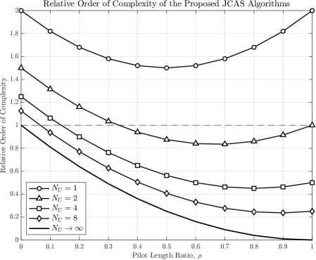
Figure 10: The relative order of complexity (given by $\frac{\text{complexity of AL-ISAC}}{\text{complexity of Bi-ISAC}}$) of the two proposed algorithms for varying values of $\rho$ and $N_{U}$.

IV-B Performance Comparison Against the State-of-the-Art

In this section, we compare the performance of the two proposed algorithms against the SotA method from [49], which also utilizes a voxelated grid to perform ISAC via leveraging multiple linear MP algorithms. We highlight, however, that the latter reference utilizes the support of a fully known intelligent reflective surface (IRS) in the ROI, and strongly relies on sparsity in the received signal, offered by means of an SCMA interface between the UEs and the AP, while our contributions are not limited to such a conditions. Instead, the proposed methods operate over fully dense received signals and with no support of IRSs.

Due to this distinction in system set-up, an adequate system parametrization must be considered for a fair comparison of our proposed algorithms against the SotA method of [49]. Specifically, in the SCMA scheme of [49], each single-antenna UE transmits an $M$-bit code by utilizing $d_{f}$ out of $R$ orthogonal frequency bands, which is received by a single AP with $N_{R}$ receive antennas. Since the considered system for our proposed algorithms is a single-frequency model (4), the diversity gain between each UE and the CPU is mimicked by setting the number of APs as $N_{A}=d_{f}$, such that $N_{A}N_{R}=d_{f}\cdot N_{R}$, such that the number of nodes and edges of the final factor graph is the same in both systems.

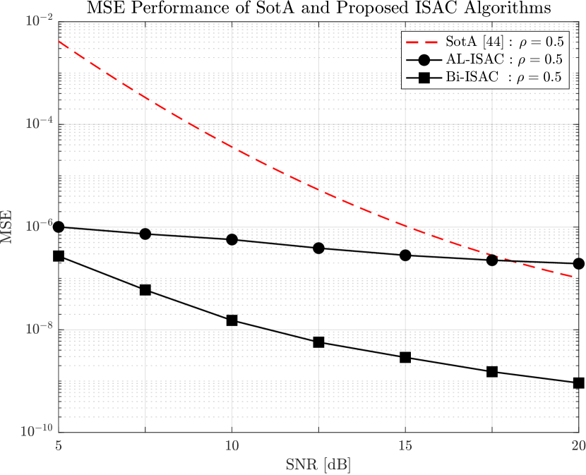
(a) MSE performance.

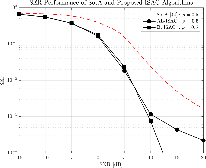
(b) SER performance.

Figure 11: MSE and SER performances of the SotA [49] against the proposed algorithms, with $N_{U}=6$, $N_{R}=9$, $N_{A}=d_{f}=2$, $N_{V}=8\times 8\times 8$, $E_{v}=1.5\%$, $M=4$, $N_{T}=100$, and $\rho=0.5$.

Fig. 11 illustrates the sensing and communication performances of the two proposed ISAC algorithms in comparison to the SotA ISAC algorithm of [49], in terms of the MSE and SERs, respectively. First, in Fig. 11(a), the sensing performance, $i.e.$, the MSE of the voxel occupancy coefficients, is evaluated. Under equivalent system parameters, in particular with a pilot ratio of $\rho=0.5$, the MSE of the proposed Bi-ISAC algorithm is found to significantly outperform that of the SotA method at all signal-to-noise ratio (SNR) values, while the AL-ISAC is found to be slightly outperformed by the latter at the high SNRs regime.

Then, in Fig. 11(b), the communication performances of the ISAC systems are evaluated in terms of the SER of the estimated symbols. It can be seen that both proposed algorithms exhibit superior symbol estimation performances compared to the SotA, with the Bi-ISAC exhibiting the additionally desirable feature that no error floors are observed even at higher SNRs.

All in all, the results corroborate the claim that both proposed methods generally outperform the SotA method of [49] in both sensing and communication functionalities.

IV-C Convergence Behavior of the Proposed Algorithms

In view of the superior performance of the two proposed ISAC algorithms in comparison with the SotA [49], we proceed in this section to further analyze the two proposed ISAC algorithms in detail, aiming also to clarify advantages of each relative to the other. To that extent, we first study the convergence behavior of the proposed ISAC algorithms so as to obtain insight on the appropriate MP termination criteria and damping parameters to be utilized.

(a) MSE convergence.

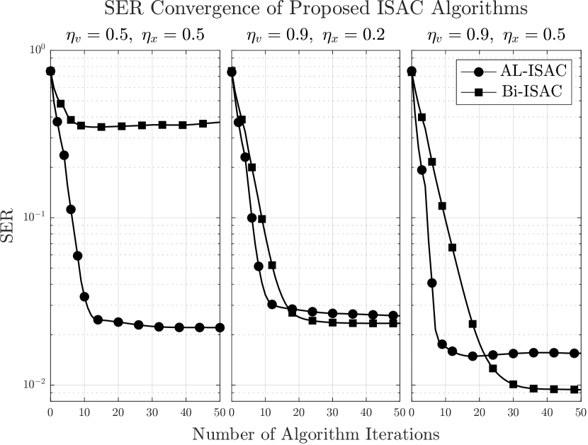
(b) SER convergence.

Figure 12: Convergence behavior of the proposed AL-ISAC and Bi-ISAC algorithms with varying damping factors $\eta_{x}$ and $\eta_{v}$ with $\rho\!=\!0.1,~{}E_{v}\!=\!1.5\%$, $\text{SNR}\!=\!15\text{dB}$, as a function of MP iterations in a system with $N_{U}=4,~{}N_{A}N_{R}=12,~{}N_{V}=512$, and $N_{T}=100$.

Figure 12 depicts the convergence behavior of the proposed ISAC algorithms in terms of the MSE of the voxel coefficient soft-replicas $\hat{v}_{k:m,t}$ and the SER of the data symbol soft-replicas $\hat{x}_{n,t:m,t}$, for three selected combinations of their respective damping parameters $\eta_{x}\in[0,1]$ and $\eta_{v}\in[0,1]$, following the damped update rule given by [69]

$$\hat{x}_{n,t:m,t}^{(\tau)}\overset{\text{update}}{\longleftarrow}\eta_{x}\!\cdot\!\hat{x}_{n,t:m,t}^{(\tau-1)}+(1-\eta_{x})\!\cdot\!\hat{x}_{n,t:m,t}^{(\tau)},~{}~{}\text{and}~{}~{}\hat{v}_{k:m,t}^{(\tau)}\overset{\text{update}}{\longleftarrow}\eta_{v}\!\cdot\!\hat{v}_{k:m,t}^{(\tau-1)}+(1-\eta_{v})\!\cdot\!\hat{v}_{k:m,t}^{(\tau)},\vspace{-0.3ex}$$ (43)

where the superscript $[\;\!\cdot\;\!]^{(\tau)}$ denotes the soft-replica at the $\tau$-th iteration of the MP loop.

It can be observed in Fig. 12(a) that while different values of $\eta_{v}$ all result in convergence of MSE, the convergent value is sensitive to the parameterization of $\eta_{v}$, especially for the Bi-ISAC which suffers from high MSE with low damping, as opposed to the AL-ISAC which is less prone to such errors in both the initial (white circles) and the final (black circles) estimation. Similar and consequent results in the SER are observed in Fig. 12(b), where convergence is also achieved in all cases, but the convergent value is largely affected by the MSE performance and $\eta_{v}$, while the effect of $\eta_{x}$ is not as prominent to the final result compared to $\eta_{v}$.

In light of the above results, the parameterization $\eta_{x}=0.5$ and $\eta_{v}=0.9$ and the convergence criteria of $\lambda=100$ iterations is selected in the following simulations to ensure a reliable convergence behavior.

IV-D Robustness Analysis of the Proposed Algorithms

To that end, we shall utilize performance metrics for the sensing and communication functions of ISAC systems other than the MSE of the estimated voxel coefficients and the SER of the estimated communication symbols, which were used in [49, 50, 51] and the previous section.

For the sensing function in particular, we remark that metrics used for radar-based ISAC cannot be used directly due to the unique voxelated occupancy grid-based approach followed here. It is therefore sensible to instead introduce a new metric, referred to as the voxel-occupancy-error-rate (VOER), which measures the rate of false-positive (FP) and false-negative (FN) elements, defined as the incorrect estimation of an occupied voxel element in presence of an empty ground-truth, and the incorrect estimation of an empty voxel element in the presence of an occupied ground-truth, respectively. Mathematically, the VOER is therefore defined as $\mathbb{E}\big{[}||\mathbf{v}-\tilde{\mathbf{v}}||_{0}\big{]}/N_{V}$, where $\mathbf{v}$ is the ground truth, $\tilde{\mathbf{v}}$ is the estimate vector, while $\|\cdot\|_{0}$ denotes the $\ell_{0}$-norm of a vector.

Notice that for the trivial all-empty (or “blind”) estimator, which returns $\tilde{\mathbf{v}}=\mathbf{0}_{N_{V}\times 1}$, the VOER reduces to $E_{v}\triangleq\mathbb{E}[||\mathbf{v}||_{0}]/N_{V}=\mathrm{VOER}_{empty}$, which is the average sparsity of the environment. We can therefore utilize this figure as an absolute reference of performance, in the sense $\mathrm{VOER}\ll\mathrm{VOER}_{empty}$ indicates a good sensing performance by a given ISAC method.

Finally, instead of the SER often used in related literature, we opt to evaluate the communication performance of the proposed ISAC schemes in terms of the more descriptive BER, defined as $\mathrm{BER}\triangleq\mathbb{E}[B_{e}]/B$, where $B_{e}$ denotes the number of errorneously detected data bits of $\mathbf{X}_{D}$, and $B$ is the total number of bits conveyed in $\mathbf{X}_{D}$.

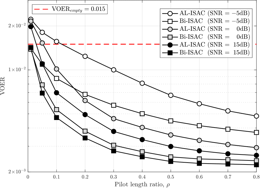
(a) Effect of pilot ratio $\rho$ for different SNRs, with fixed environment sparsity $E_{v}=1.5\%$ and SNR $=15\mathrm{dB}$.

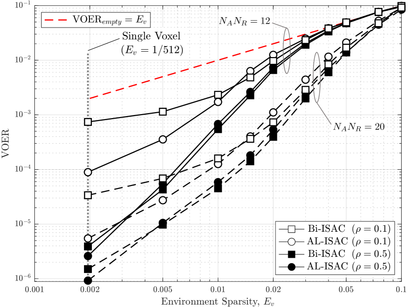
(b) Effect of environment sparsity $E_{v}$ with varying pilot ratio $\rho$, with fixed SNR $=15\mathrm{dB}$.

Figure 13: VOER performance of the proposed AL-ISAC and Bi-ISAC algorithms in a system with $N_{U}=4,~{}N_{A}N_{R}=12,~{}N_{V}=512$, and $N_{T}=100$.

First, we evaluate the robustness of the two proposed algorithms in terms of their VOER performances, as a function of different system parameters including the pilot ratio $\rho$, SNR, and environment sparsity $E_{v}$ (voxel occupancy probability).

In Fig. 13(a), the effect of varying the pilot ratio $\rho$ is illustrated for various SNRs. The results show that, for a specific value of $\rho$, the Bi-ISAC outperforms the AL-ISAC for the entire SNR range; or alternatively, that for a given SNR, the Bi-ISAC scheme requires a much lower number of pilots to achieve the same VOER performance of the AL-ISAC method. Next, Fig. 13(b) depicts the effect of environment sparsity $E_{v}$ on the VOER performance of the proposed algorithms, where it is observed that the AL-ISAC can actually achieve a superior performance over the Bi-ISAC in extremely sparse environments as can be seen in the single voxel case of $E_{v}=1/512\approx 0.002$. On the other hand, the Bi-ISAC is more robust in the sense that it exhibits smaller gradient, which suggests that the Bi-ISAC is less affected by changes in $E_{v}$. The Bi-ISAC also tends to outperform the AL-ISAC as $E_{v}$ increases (i.e., for $E_{v}>0.01$).

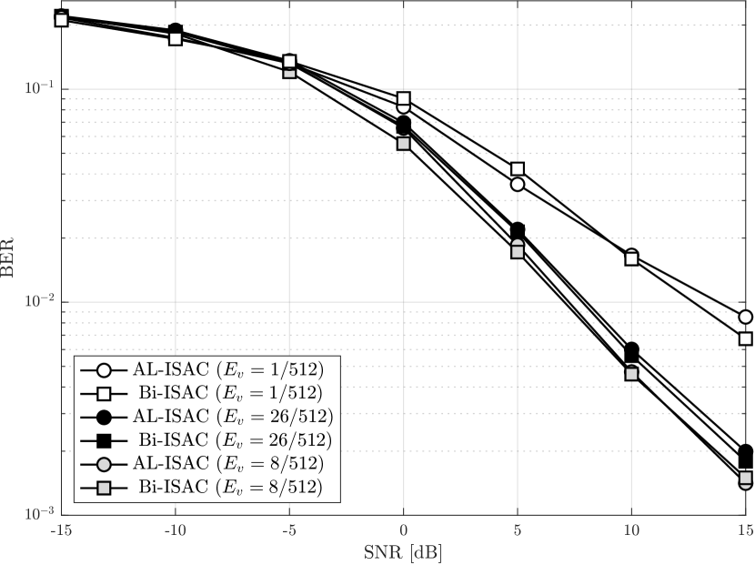
(a) Effect of environment sparsity $E_{v}$ and SNR, with fixed pilot ratio $\rho=0.1$.

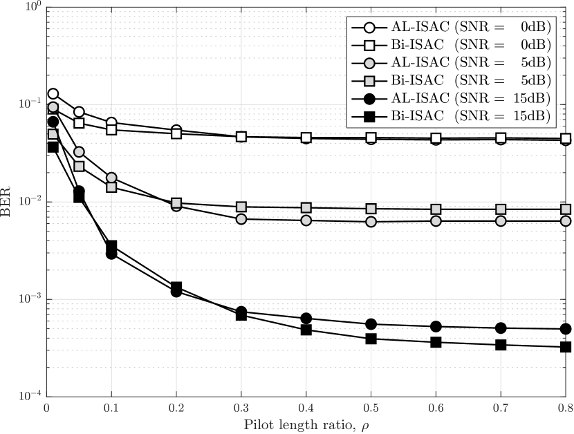
(b) Effect of pilot ratio $\rho$ for different SNRs, with fixed environment sparsity $E_{v}=1.5\%$.

Figure 14: BER performance of the proposed AL-ISAC and Bi-ISAC algorithms in a system with $N_{U}=4,~{}N_{A}N_{R}=12,~{}N_{V}=512$, and $N_{T}=100$.

Next, we proceed to evaluate the BER performance of the proposed algorithms, which are compared in Fig. 14(a) as a function of the SNR and for different environment sparsities, namely $E_{v}=0.002,0.015,0.05$, which respectively correspond to $1,8,$ and $26$ occupied voxels (out of $512$ total) in the environment. Since the VOER performance as seen in Fig. 13 degrades with larger $E_{v}$, one may expect the BER performance to follow the same behavior. However, it is observed that an extremely sparse environment results in BER performance degradation.

While counter-intuitive at a first sight, these results are actually intuitive if analyzed from an information/estimation-theoretical viewpoint. Although fundamental limits on the performances of ISAC are still to be derived, it is to be expected that with a certain amount of resources such as power, side information ($i.e.$, pilot signals) and computational complexity, a fundamental limit on the joint estimation and communications performances exists. Indeed, from an algorithmic viewpoint, a large number of voxels implies that much of the degrees-of-freedom are utilized for environment estimation, which negatively impacts the communications performance. Similarly, an extremely sparse environment implies that most voxel coefficients are $0$, such that the corresponding connected edges in the factor graph are nullified, deteriorating BER performance.

Next, Fig. 14(b) evaluates the effect of the pilot ratio on the BER performance, where it can be seen that for small pilot ratios (i.e., $\rho<0.2$), the two proposed algorithms achieve a similar performance, but that for larger pilot ratios (i.e., $\rho>0.3$), the AL-ISAC outperforms the Bi-ISAC in moderate SNR cases (i.e., $5\mathrm{dB}$). This result, which can be counter-intuitive to the reader, is actually expected and explained by the fact that linear MP modules of the AL-ISAC scheme are constructed on the assumption of perfect symbol knowledge (0 uncertainty for symbol estimates), whose assumptions are increasing met with large pilot ratios. Ultimately, however, at significantly high SNRs (i.e., SNR $\geq 15\mathrm{dB}$), the Bi-ISAC is again shown to outperform AL-ISAC, which is a direct consequence of the error-floor behavior exhibited by the AL-ISAC algorithm.

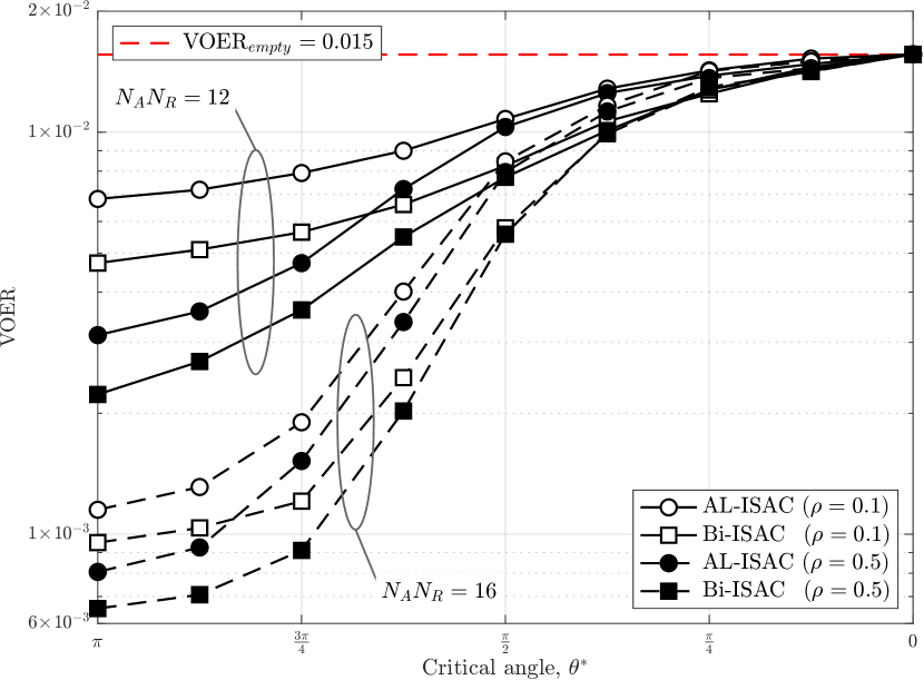
(a) VOER performance.

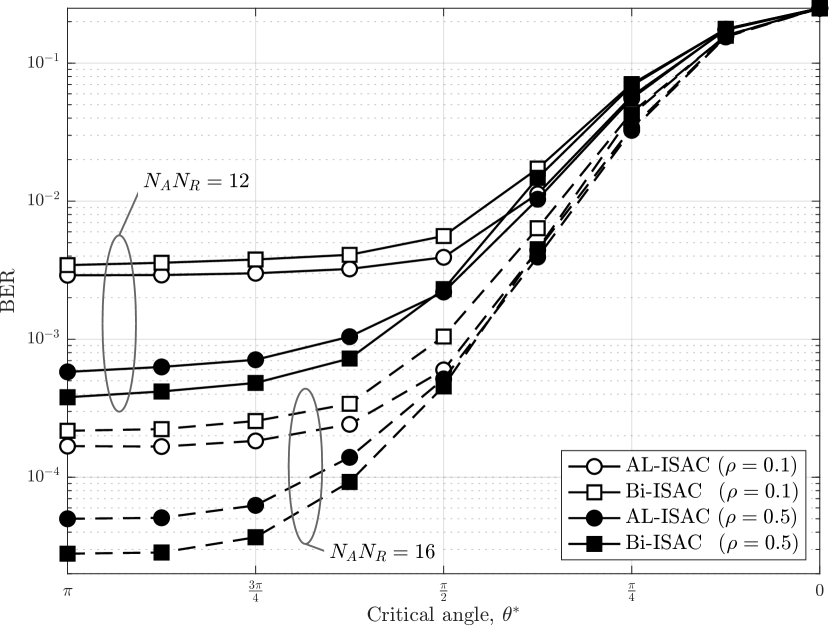
(b) BER performance.

Figure 15: Performance of the proposed AL-ISAC and Bi-ISAC algorithms with varying pilot ratios $\rho$, with $E_{v}=1.5\%,~{}\text{SNR}=15\text{dB}$, as a function of the critical channel blockage angle $\theta^{*}$.

Finally, Fig. 15 elucidates the effect of random channel blockages as discussed in Section II-C. In particular, the figure compares the VOER and BER performances of the two proposed ISAC algorithms with respect to the critical angle $\theta^{*}$, which determines the channel blockage rate following the stochastic-geometric empirical model derived in Sec. II-C (see Fig. 4).

The environment sensing performance illustrated in Fig. 15(a) exhibits a similar behavior to the effect of $\rho$, where the Bi-ISAC achieves a superior performance for all cases. In addition, the Bi-ISAC curves exhibit a slower increase in gradient compared to those of AL-ISAC, which indicates the higher robustness of Bi-ISAC to path blockages. The superior robustness of the Bi-ISAC algorithm against both pilot length and random channel blockages can be accredited to the increased number of edges in the full factor graph arising from the bilinear representation of the system, which can be seen by comparing Fig. 5 and Fig. 6 of the linear case against Fig. 9 of the bilinear case. Each factor node of the bilinear factor graph is connected to a significantly larger number of variable nodes as compared to the linear factor graphs, which implies more remaining edges for stable message passing even when a large number of edges are removed. MP over the pruned graph is only feasible when there are sufficient pilot data still connected to the main graph, therefore making the Bi-ISAC more dependent on the pilot ratio for stability.

As for the communications performances, compared in Fig. 15(b), it is found that the behavior of both schemes differ with the pilot ratio. For low pilot ratios, the AL-ISAC is shown to slightly outperform the Bi-ISAC, whereas for high pilot ratios, the Bi-ISAC exhibits a more significantly superior performance to the AL-ISAC, further corroborating the results of Fig. 13(a).

 

V Conclusion

We proposed two new ISAC schemes in which a voxelated 3D representation of a ROI is extracted from the scattering features present in the effective CSI, utilizing the same physical layer communications air interface of an uplink connection between multiple single-antenna UEs and multi-antenna APs. The first scheme, dubbed AL-ISAC, relies on a modular feedback structure in which the transmit data and the environment are estimated alternately, whereas the second method, referred to as Bi-ISAC, leverages the bilinear inference framework to estimate both variables concurrently. Both contributed methods were shown via computer simulations to outperform the SotA in accurately recovering the transmitted data, as well as in obtaining a voxelated 3D image of the environment. An analysis of the computational complexities and robustness of the proposed methods revealed distinct advantages of each scheme, namely, that Bi-ISAC exhibits an overall best performance and robustness to short pilots and channel blockages, while AL-ISAC offers lower complexity especially in scenarios with large numbers of UEs, and can exhibit superior performance under ideal conditions such as long pilot blocks, high environment sparsity, and no channel blockages.

References

- [1]
- [2]
- [3] H. S. Rou, G. T. F. Abreu, D. Gonzalez G., and O. Gonsa, “Asymmetric bilinear inference for joint communications and environment sensing,” in 2022 56th Asilomar Conference on Signals, Systems, and Computers, 2022, pp. 1111–1115.
- [4] W. Saad, M. Bennis, and M. Chen, “A vision of 6G wireless systems: Applications, trends, technologies, and open research problems,” IEEE Network, vol. 34, no. 3, pp. 134–142, 2020.
- [5] Z. Zhang et al., “6G wireless networks: Vision, requirements, architecture, and key technologies,” IEEE Veh. Technol. Mag., vol. 14, no. 3, pp. 28–41, 2019.
- [6] T. S. Rappaport et al., “Overview of millimeter wave communications for fifth-generation (5G) wireless networks—with a focus on propagation models,” IEEE Trans. Antennas Propag., vol. 65, no. 12, pp. 6213–6230, 2017.
- [7] X. Wang et al., “Millimeter wave communication: A comprehensive survey,” IEEE Commun. Surveys Tuts., vol. 20, no. 3, pp. 1616–1653, 2018.
- [8] M. Xiao et al., “Millimeter wave communications for future mobile networks,” IEEE J. Sel. Areas Comm., vol. 35, no. 9, pp. 1909–1935, 2017.
- [9] Y. Niu et al., “A survey of millimeter wave communications (mmWave) for 5G: opportunities and challenges,” Wireless Networks, vol. 21, no. 8, pp. 2657–2676, 2015.
- [10] H.-J. Song and N. Lee, “Terahertz communications: Challenges in the next decade,” IEEE Trans. THz Sci. Technol., vol. 12, no. 2, pp. 105–117, 2022.
- [11] H. Elayan et al., “Terahertz communication: The opportunities of wireless technology beyond 5G,” in 2018 International Conference on Advanced Communication Technologies and Networking (CommNet), 2018, pp. 1–5.
- [12] T. S. Rappaport et al., “Wireless communications and applications above 100 GHz: Opportunities and challenges for 6G and beyond,” IEEE Access, vol. 7, pp. 78 729–78 757, 2019.
- [13] J. Zhang, S. Chen, Y. Lin, J. Zheng, B. Ai, and L. Hanzo, “Cell-free massive MIMO: A new next-generation paradigm,” IEEE Access, vol. 7, pp. 99 878–99 888, 2019.
- [14] E. D. Carvalho, A. Ali, A. Amiri, M. Angjelichinoski, and R. W. Heath, “Non-stationarities in extra-large-scale massive MIMO,” IEEE Wireless Commun., vol. 27, no. 4, pp. 74–80, 2020.
- [15] M. Wang, F. Gao, S. Jin, and H. Lin, “An overview of enhanced massive MIMO with array signal processing techniques,” IEEE J. Sel. Topics in Signal Process., vol. 13, no. 5, pp. 886–901, 2019.
- [16] E. Basar et al., “Wireless communications through RISs,” IEEE Access, vol. 7, pp. 116 753–116 773, 2019.
- [17] Q. Wu and R. Zhang, “Intelligent reflecting surface enhanced wireless network via joint active and passive beamforming,” IEEE Trans. Wireless Commun., vol. 18, no. 11, pp. 5394–5409, 2019.
- [18] C. Huang et al., “Reconfigurable intelligent surfaces for energy efficiency in wireless communication,” IEEE Trans. Wireless Commun., vol. 18, no. 8, pp. 4157–4170, 2019.
- [19] F. Liu et al., “Integrated sensing and communications: Toward dual-functional wireless networks for 6G and beyond,” IEEE J. Sel. Areas Commun., vol. 40, no. 6, pp. 1728–1767, 2022.
- [20] A. Liu et al., “A survey on fundamental limits of integrated sensing and communication,” IEEE Commun. Surveys Tuts., vol. 24, no. 2, pp. 994–1034, 2022.
- [21] Z. Xiao and Y. Zeng, “Full-duplex integrated sensing and communication: Waveform design and performance analysis,” in 2021 13th International Conference on Wireless Communications and Signal Processing (WCSP), 2021, pp. 1–5.
- [22] R. Thomä et al., “Joint communication and radar sensing: An overview,” in 2021 15th EuCAP Conf., 2021, pp. 1–5.
- [23] T. Wild, V. Braun, and H. Viswanathan, “Joint design of communication and sensing for beyond 5G and 6G systems,” IEEE Access, vol. 9, pp. 30 845–30 857, 2021.
- [24] J. A. Zhang et al., “An overview of signal processing techniques for joint communication and radar sensing,” IEEE J. Sel. Topics Sig. Proc., vol. 15, no. 6, pp. 1295–1315, 2021.
- [25] J. A. Zhang et al., “Enabling joint communication and radar sensing in mobile networks - a survey,” IEEE Commun. Surveys Tuts., vol. 24, no. 1, pp. 306–345, 2022.
- [26] F. Liu et al., “Joint radar and communication design: Applications, state-of-the-art, and the road ahead,” IEEE Trans. Commun., vol. 68, no. 2, pp. 3834–3982, 2020.
- [27] Y. Zeng and X. Xu, “Toward environment-aware 6G communications via channel knowledge map,” IEEE Wireless Commun., vol. 28, no. 3, pp. 84–91, 2021.
- [28] A. Dulaimi and X. Lin, “Reshaping autonomous driving for 6G era,” IEEE Comm. Std. Mag., vol. 4, no. 1, pp. 10, 2020.
- [29] D. Mishra, A. M. Vegni, V. Loscrí, and E. Natalizio, “Drone networking in the 6G era: A technology overview,” IEEE Commun. Standards Mag., vol. 5, no. 4, pp. 88–95, 2021.
- [30] Y. Xing, O. Kanhere, S. Ju, and T. S. Rappaport, “Indoor wireless channel properties at millimeter wave and sub-terahertz frequencies,” in 2019 IEEE Global Communications Conference (GLOBECOM), 2019, pp. 1–6.
- [31] S. Kanaun, Heterogeneous Media: Local Fields, Effective Properties, and Wave Propagation, ser. Elsevier Series in Mechanics of Adv. Materials. Elsevier, 2020.
- [32] G. Charan, M. Alrabeiah, and A. Alkhateeb, “Vision-aided 6G wireless communications: Blockage prediction and proactive handoff,” IEEE Trans. Veh. Technol., vol. 70, no. 10, pp. 10 193–10 208, Aug. 2021.
- [33] L. Yu, J. Zhang, Y. Zhang, X. Li, and G. Liu, “Long-range blockage prediction based on diffraction fringe characteristics for mmWave communications,” IEEE Commun. Lett., pp. 1–1, 2022.
- [34] S. Wu, M. Alrabeiah, C. Chakrabarti, and A. Alkhateeb, “Blockage prediction using wireless signatures: Deep learning enables real-world demonstration,” IEEE Open Journ. Commun. Soc., vol. 3, pp. 776–796, Mar. 2022.
- [35] M. A. Richards, Fundamentals of Radar Signal Processing. McGraw-Hill, 2014.
- [36] T. Long, Z. Liang and Q. Liu, “Advanced technology of high-resolution radar: target detection, tracking, imaging, and recognition,” Sci. China Inf. Sci., vol. 62, pp. 1–26, 2019.
- [37] L. Zheng, M. Lops, Y. C. Eldar, and X. Wang, “Radar and communication coexistence: An overview: A review of recent methods,” IEEE Signal Process. Mag., vol. 36, no. 5, pp. 85–99, 2019.
- [38] F. Liu, C. Masouros, A. Li, T. Ratnarajah, and J. Zhou, “MIMO radar and cellular coexistence: A power-efficient approach enabled by interference exploitation,” IEEE Trans. Signal Process., vol. 66, no. 14, pp. 3681–3695, 2018.
- [39] T. Huang, N. Shlezinger, X. Xu, Y. Liu, and Y. C. Eldar, “MAJoRCom: A dual-function radar communication system using index modulation,” IEEE Trans. on Signal Process., vol. 68, pp. 3423–3438, 2020.
- [40] D. Ma, N. Shlezinger, T. Huang, Y. Liu, and Y. C. Eldar, “FRaC: FMCW-based joint radar-communications system via index modulation,” IEEE J. Sel. Topics Signal Process., vol. 15, no. 6, pp. 1348–1364, 2021.
- [41] P. Kumari, J. Choi, N. González-Prelcic and R. W. Heath, “IEEE 802.11ad-based radar: An approach to joint vehicular communication-radar system,” IEEE Trans. Veh. Technol., vol. 67, no. 4, pp. 3012–3027, 2018.
- [42] Y. Liu, G. Liao, and Z. Yang, “Range and angle estimation for MIMO-OFDM integrated radar and communication systems,” in 2016 CIE International Conference on Radar (RADAR), 2016, pp. 1–4.
- [43] P. Raviteja, K. T. Phan, Y. Hong, and E. Viterbo, “Orthogonal time frequency space (OTFS) modulation based radar system,” in 2019 IEEE Radar Conference (RadarConf), 2019, pp. 1–6.
- [44] X. Yuan et al., “Spatio-temporal power optimization for MIMO joint communication and radio sensing systems with training overhead,” IEEE Trans. Veh. Technol., vol. 70, no. 1, pp. 514–528, 2021.
- [45] Y. Liu et al., “Adaptive OFDM integrated radar and communications waveform design based on information theory,” IEEE Commun. Let., vol. 21, no. 10, pp. 2174–2177, 2017.
- [46] Y. Luo, J. A. Zhang, X. Huang, W. Ni, and J. Pan, “Multibeam optimization for joint communication and radio sensing using analog antenna arrays,” IEEE Trans. Veh. Technol., vol. 69, no. 10, pp. 11 000–11 013, 2020.
- [47] B. Tan et al., “Exploiting WiFi channel state information for residential healthcare informatics,” IEEE Commun. Mag., vol. 56, no. 5, pp. 130–137, 2018.
- [48] S. Yousefi et al., “A survey on behavior recognition using WiFi channel state information,” IEEE Commun. Mag., vol. 55, no. 10, pp. 98–104, 2017.
- [49] X. Tong et al., “Joint multi-user communication and sensing exploiting both signal and environment sparsity,” IEEE J. Sel. Topics Signal Process., vol. 15, no. 6, pp. 1409–1422, 2021.
- [50] Y. Tao and Z. Zhang, “Distributed computational imaging with reconfigurable intelligent surface,” in 2020 International Conference on Wireless Communications and Signal Processing (WCSP), 2020, pp. 448–454.
- [51] Y. Zhang, Z. Zhang, X. Tong, and C. W. Huang, “3D environment sensing with channel state information based on computational imaging,” in 2022 IEEE ICC Workshops, 2022, pp. 842–847.
- [52] I. Tropkina, A. Pyattaev, Y. Sadovaya, and S. Andreev, “Modeling of SHF/EHF radio-wave scattering for curved surfaces with voxel cone tracing,” IEEE Antennas and Wireless Propag. Lett., vol. 21, no. 2, pp. 426–430, 2022.
- [53] N. Morales et al., “A combined voxel and particle filter-based approach for fast obstacle detection and tracking in automotive applications,” IEEE Trans. Intell. Transp. Syst., vol. 18, no. 7, pp. 1824–1834, 2017.
- [54] K. Pirker, M. Rüther, H. Bischof, and G. Schweighofer, “Fast and accurate environment modeling using three-dimensional occupancy grids,” in 2011 IEEE ICCV Workshops, 2011, pp. 1134–1140.
- [55] T. Collins et al., “Occupancy grid mapping: An empirical evaluation,” in 2007 MCCA Conf., 2007, pp. 1–6.
- [56] D. He, et al., “The design and applications of high-performance ray-tracing simulation platform for 5G and beyond wireless communications: A tutorial,” IEEE Commun. Surveys Tuts, vol. 21, no. 1, pp. 10–27, 2019.
- [57] H. Choi and J. Choi, “WiThRay: Versatile 3D simulator for intelligent reflecting surface-aided mmWave systems,” in 2021 International Symposium on Antennas and Propagation (ISAP), 2021, pp. 1–2.
- [58] C. Tu, E. Takeuchi, A. Carballo, and K. Takeda, “Point cloud compression for 3D lidar sensor using recurrent neural network with residual blocks,” in 2019 ICRA Conf., 2019, pp. 3274–3280.
- [59] V. Degli-Esposti et al., Special Issue: mmWave and THz Propag., Chan. Mod., and Appli. IEEE Access, 2021, vol. 9.
- [60] G. Kang, “Time and frequency domain joint channel estimation in multi-carrier multi-branch systems,” Ph.D. dissertation, Technischen Universität Kaiserslautern, 2005.
- [61] J. Møller and D. Stoyan, “Stochastic geometry and random tessellations,” 2007.
- [62] V. Sadílek and M. Vořechovský, “Evaluation of pairwise distances among points forming a regular orthogonal grid in a hypercube,” Jounr. of Civil Engineering and Management, vol. 24, no. 5, pp. 410–428, Sep. 2018.
- [63] J. T. Parker, P. Schniter, and V. Cevher, “Bilinear generalized approximate message passing—part I: Derivation,” IEEE Trans. Signal Process., vol. 62, no. 22, pp. 5839–5853, 2014.
- [64] H. Iimori et al., “Grant-free access via bilinear inference for cell-free MIMO with low-coherence pilots,” IEEE Trans. Wireless Commun., vol. 20, no. 11, pp. 7694–7710, 2021.
- [65] H. Iimori et al., “Grant-free access for extra-large MIMO systems subject to spatial non-stationarity,” in ICC 2022 - IEEE International Conference on Communications, 2022, pp. 1758–1762.
- [66] J. T. Parker and P. Schniter, “Parametric bilinear generalized approximate message passing,” IEEE J. Sel. Topics Signal Process., vol. 10, no. 4, pp. 795–808, 2016.
- [67] Z. Yuan, Q. Guo, and M. Luo, “Approximate message passing with unitary transformation for robust bilinear recovery,” IEEE Trans. Signal Process., vol. 69, pp. 617–630, 2021.
- [68] H. S. Rou, G. T. F. Abreu, and T. Takahashi, “An efficient vector-valued belief propagation decoder for quadrature spatial modulation,” in 56th Asilomar Conference on Signals, Systems, and Computers, 2022, pp. 27–31.
- [69] P. Som, T. Datta, A. Chockalingam and B. S. Rajan, “Improved large-MIMO detection based on damped belief propagation,” in IEEE Inf. Theory Workshop on Inf. Theory, 2010, pp. 1–5.
- [70] M. Taherzadeh, H. Nikopour, A. Bayesteh, and H. Baligh, “SCMA codebook design,” in 2014 IEEE 80th Vehicular Technology Conference (VTC2014-Fall), 2014, pp. 1–5.