UniM²AE: Multi-modal Masked Autoencoders with Unified 3D Representation for 3D Perception in Autonomous Driving

Abstract

Masked Autoencoders (MAE) play a pivotal role in learning potent representations, delivering outstanding results across various 3D perception tasks essential for autonomous driving. In real-world driving scenarios, it’s commonplace to deploy multiple sensors for comprehensive environment perception. While integrating multi-modal features from these sensors can produce rich and powerful features, there is a noticeable gap in MAE methods addressing this integration. This research delves into multi-modal Masked Autoencoders tailored for a unified representation space in autonomous driving, aiming to pioneer a more efficient fusion of two distinct modalities. To intricately marry the semantics inherent in images with the geometric intricacies of LiDAR point clouds, the UniM²AE is proposed. This model stands as a potent yet straightforward, multi-modal self-supervised pre-training framework, mainly consisting of two designs. First, it projects the features from both modalities into a cohesive 3D volume space, ingeniously expanded from the bird’s eye view (BEV) to include the height dimension. The extension makes it possible to back-project the informative features, obtained by fusing features from both modalities, into their native modalities to reconstruct the multiple masked inputs. Second, the Multi-modal 3D Interactive Module (MMIM) is invoked to facilitate the efficient inter-modal interaction during the interaction process. Extensive experiments conducted on the nuScenes Dataset attest to the efficacy of UniM²AE, indicating enhancements in 3D object detection and BEV map segmentation by 1.2%(NDS) and 6.5% (mIoU), respectively. Code is available at https://github.com/hollow-503/UniM2AE.

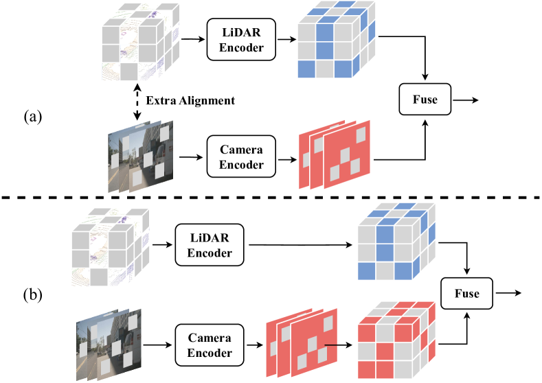
Figure 1: (a) Multi-modal frameworks [1] that align masked input before feature extraction but ignore feature characteristics from two branch. (b) UniM²AE that interacts multi-modal features with unified representation.

I Introduction

Autonomous driving marks a transformative leap in transportation, heralding potential enhancements in safety, efficiency, and accessibility. Fundamental to this progression is the vehicle’s capability to decode its surroundings. To tackle the intricacies of real-world contexts, integration of various sensors is imperative: cameras yield detailed visual insights, LiDAR grants exact geometric data, etc.Through this multi-sensor fusion, a comprehensive grasp of the environment is achieved. While current Masked Autoencoders (MAE) excel at learning robust representations for a single modality  [2, 3], they struggle to effectively combine the semantic depth of images with the geometric nuances of LiDAR point clouds, especially in the realm of autonomous driving. This limitation presents an obstacle to attaining the nuanced understanding necessary for crafting robust and potent representations.

MAE has shown notable success in 2D vision [4, 5, 6]. Some self-supervised frameworks, such as [7], attempt to use 2D pre-trained knowledge to inform 3D MAE pre-training. However, these efforts yield only minor performance enhancements, primarily due to challenges in bridging 2D and 3D data spaces. On the other hand, as shown in Figure 1 (a), methods like PiMAE [1] focus on directly fusing 2D and 3D data. However, these approaches often neglect the nuances between indoor and outdoor scenes. Such oversight complicates their application in autonomous driving contexts, which are characterized by extensive areas and intricate occlusion relationships.

To address the identified challenges, UniM²AE is introduced as a self-supervised pre-training framework optimized for integrating two distinct modalities: images and LiDAR data. The strategy aims to establish a unified representation space, enhancing the fusion of these modalities as shown in Figure 1 (b). In this framework, the semantic richness of images is seamlessly merged with the geometric details captured by LiDAR to produce a robust and informative feature.

The transformation to a 3D volume space is a critical step in ensuring comprehensive interaction between the multi-modal data sources. Starting with the LiDAR data, it’s processed into voxels and given a specific embedding through DynamicVFE, a method known for its efficacy in handling LiDAR data as mentioned in [8]. In parallel, images undergo a division process where they’re segmented into patches. These patches are then embedded using positional embeddings, ensuring spatial relationships are preserved. Upon these initial processing steps, the multi-view images and voxelized LiDAR point clouds are then interpreted and encoded by their designated encoders. The output from both encoders is then integrated into a unified 3D volume space. Not only does it ensure the maintenance of both geometric and semantic nuances, but it also accommodates an additional height dimension. This height element plays a pivotal role in the process. It grants the capability to reverse project the features back to their original modalities, enabling the reconstruction of the initially masked inputs from the various data branches.

Compared with indoor scenes, scenarios in autonomous driving are generally expansive, encompassing a greater number of objects and displaying intricate inter-instance relationships. The Multi-modal 3D Interaction Module (MMIM) is employed to amalgamate features from the dual branches to facilitate efficient interaction. This module is built upon stacked 3D deformable self-attention blocks, enabling the modeling of global context at elevated resolutions.

Comprehensive experiments on nuScenes [9] demonstrate that our pre-training method significantly enhances the model’s performance and convergence speed in downstream tasks. Specifically, our UniM²AE improves detection performance by 1.2/1.5 NDS/mAP even with larger voxel size and promotes BEV map segmentation performance by 6.5 mAP. According to our ablation study, it also reduces training time almost by half when utilizing the entire dataset.

To sum up, our contributions can be presented as follows:

• We propose UniM²AE, a multi-modal self-supervised pre-training framework with unified representation in a cohesive 3D volume space. This representation advantageously allows for feature transformation back to the original modality, facilitating the reconstruction of multi-modal masked inputs.

• To better interact semantics and geometries retained in unified 3D volume space, we introduce a Multi-modal 3D Interaction Module (MMIM) to obtain more informative and powerful features.

• We conduct extensive experiments on various 3D downstream tasks, where UniM²AE notably promotes diverse detectors and shows competitive performance.

II Related Work

II-A Multi-Modal Representation

Multi-modal representation has raised significant interest recently, especially in vision-language pre-training [10, 11]. Some works [12, 13] align point cloud data to 2D vision by depth projection. As for unifying 3D with other modalities, the bird’s-eye view (BEV) is a widely-used representation since the transformation to BEV space retains both geometric structure and semantic density. Although many SOTA methods [14, 15] adopt BEV as the unified representation, the lack of height information leads to a poor description of the shape and position of objects, which makes it unsuitable for MAE. In this work, we introduce a unified representation with height dimension in 3D volume space, which captures the detailed height and position of objects.

II-B Masked Autoencoders

Masked Autoencoders (MAE) [6] are a self-supervised pre-training method, with a pre-text task of predicting masked pixels. With its success, a series of 3D representation learning methods apply masked modeling to 3D data. Some works [16, 2, 17] reconstruct masked points of indoor objects. Some works [18, 3, 19, 20, 21] predict the masked voxels in outdoor scenes. Recent methods propose multi-modal MAE pre-training: [7] exploits 2D pre-trained knowledge to the 3D point prediction but fails to exploit the full potential of LiDAR point cloud and image datasets. [1] attempts to tackle it in the indoor scene and conducts a 2D-3D joint prediction by the projection of points but ignore the characteristic of point clouds and images. To address these problems, we propose to predict both masked 2D pixels and masked 3D voxels in a unified representation, focusing on the autonomous driving scenario.

II-C Multi-Modal Fusion in 3D Perception

Recently, multi-modal fusion has been well-studied in 3D perception. Proposal-level fusion methods adopt proposals in 3D and project the proposals to images to extract RoI feature [22, 23, 24]. Point-level fusion methods usually paint image semantic features onto foreground LiDAR points, which can be classified into input-level decoration  [25, 26, 27], and feature-level decoration  [28, 29]. However, the camera-to-LiDAR projection is semantically lossy due to the different densities of both modalities. Some BEV-based approaches aim to mitigate this problem, but their simple fusion modules fall short in modeling the relationships between objects. Accordingly, we design the Multi-modal 3D Interaction Module to effectively fuse the projected 3D volume features.

III Method

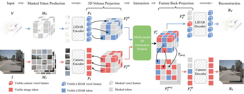
Figure 2: Pre-training overview of UniM²AE. The LiDAR branch voxelize the point cloud, while the camera branch divides multiple images into patches, both subsequently randomly masking their inputs. The tokens from the two branches are individually embedded and then passed through the Token-Volume projection, Multi-modal 3D Interaction Module, Volume-Token projection, and eventually the modality-specific decoder. Ultimately, we reconstruct the original inputs using the fused features.

In this section, we initially present an overview of our UniM²AE, specifically focusing on the pre-training phase. Sequentially, we then detail unified representation in 3D volume space and the operations of our integral sub-modules, which include representation transformation, multi-modal interaction, and reconstruction.

III-A Overview Architecture

As shown in Figure 2, UniM²AE learns multi-modal representation by masking inputs $(I,V)$ and jointly combine features projected to the 3D volume space $(F^{vol}_{V},F^{vol}_{I})$ to accomplish the reconstruction. In our proposed pipeline, the point cloud is first embeded into tokens after voxelization and similarly we embed the images with position encoding after dividing the them into non-overlapping patches. Following this, tokens from both modalities are randomly masked, producing $(M_{I},M_{V})$. Separate transformer-based encoders are then utilized to extract features $(F_{I},F_{V})$.

To align features from various modalities with the preservation of semantics and geometrics, $(F_{I},F_{V})$ are separately projected into the unified 3D volume space, which is extended BEV along the height dimension. Specifically, we build a mapping of each voxel to 3D volume space based on its position in the ego-vehicle coordinates, while for the image tokens, the spatial cross-attention is employed for 2D to 3D conversion. The projected feature $(F^{vol}_{V},F^{vol}_{I})$ are subsequently passed into the Multi-modal 3D Interaction Module (MMIM), aiming at promoting powerful feature fusion.

Following the cross-modal interaction, we project the fused feature $F^{\prime}_{c}$ back to the modality-specific token, denoted $F^{sp}_{V}$ for LiDAR and $F^{proj}_{I}\in(C,H,W)$ (which is then reshaped to $F^{sp}_{I}\in(HW,C)$) for camera. The camera decoder and LiDAR decoder are finally used to reconstruct the original inputs.

III-B Unified Representation in 3D volume space

Different sensors capture data that, while representing the same scene, often provide distinct descriptions. For instance, camera-derived images emphasize the color palette of the environment within their field of view, whereas point clouds primarily capture object locations. Given these variations, selecting an appropriate representation for fusing features from disparate modalities becomes paramount. Such a representation must preserve the unique attributes of multi-modal information sourced from various sensors.

In pursuit of capturing the full spectrum of object positioning and appearance, the voxel feature in 3D volume space is adopted as the unified representation, depicted in Figure 1 (b). The 3D volume space uniquely accommodates the height dimension, enabling it to harbor more expansive geometric data and achieve exacting precision in depicting object locations, exemplified by features like elevated traffic signs. This enriched representation naturally amplifies the accuracy of interactions between objects. A salient benefit of the 3D volume space is its capacity for direct remapping to original modalities, cementing its position as an optimal latent space for integrating features. Due to the intrinsic alignment of images and point clouds within the 3D volume space, the Multi-modal 3D Interaction Module can bolster representations across streams, sidestepping the need for additional alignment mechanisms. Such alignment streamlines the transition between pre-training and fine-tuning stages, producing favorable outcomes for subsequent tasks. Additionally, the adaptability of the 3D volume space leaves the door open for its extension to encompass three or even more modalities.

III-C Multi-modal Interaction

III-C1 Projection to 3D volume space

In the projection of LiDAR to the 3D volume, the voxel embedding is directed to a predefined 3D volume using positions from the ego car coordinate system. This method ensures no geometric distortion is introduced. The resulting feature from this process is denoted as ${F}^{vol}_{V}$. For the image to 3D volume projection, the 2D-3D Spatial Cross-Attention method is employed. Following prior works [30, 31], 3D volume queries for each image is defined as $Q^{vol}\in\mathbf{R}^{C\times H\times W\times Z}$. The corresponding 3D points are then projected to 2D views using the camera’s intrinsic and extrinsic parameters. During this projection, the 3D points associate only with specific views, termed as $\mathcal{V}_{hit}$. The 2D feature is then sampled from the view $\mathcal{V}_{hit}$ at the locations of those projected 3D reference points. The process unfolds as:

$$F^{vol}_{I}=\frac{1}{\left|\mathcal{V}_{hit}\right|}\sum_{i\in\mathcal{V}_{hit}}\sum_{j=1}^{N_{ref}}\mathrm{DeformAttn}\left(Q^{vol},\mathcal{P}(p,i,j),F_{I}^{i}\right)$$ (1)

where $i$ indexes the camera view, $j$ indexes the 3D reference points, and $N_{ref}$ is the total number of points for each 3D volume query. $F_{I}^{i}$ is the features of the $i$-th camera view. $\mathcal{P}(p,i,j)$ is the project function that gets the $j$-th reference point on the $i$-th view image.

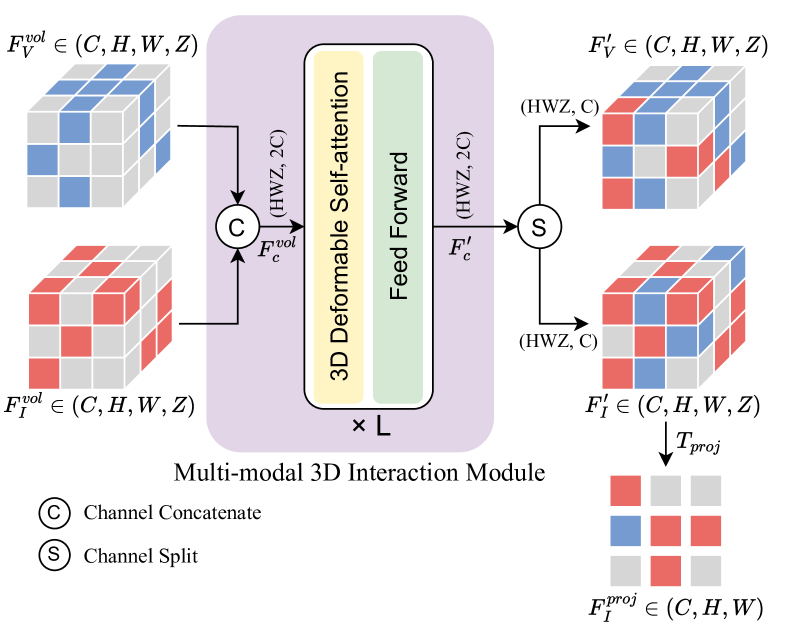
Figure 3: Illustration of our Multi-modal 3D Interaction Module. We first concatenate the inputs $\left(F_{V}^{vol},F_{I}^{vol}\right)$ and reshape it for the subsequent stacking 3D deformable self-attention blocks. After interaction, we split the output volume feature and project them back to feature token. This contributes more generalized and effective feature learning.

III-C2 Multi-modal 3D Interaction Module

To fuse the projected 3D volume features from the camera ($F^{vol}_{I}\in\mathbf{R}^{C\times H\times W\times Z}$) and the LiDAR ($F^{vol}_{V}\in\mathbf{R}^{C\times H\times W\times Z}$) branches effectively, the Multi-modal 3D Interaction Module (MMIM) is introduced. As depicted in Figure 3, MMIM comprises $L$ attention blocks, with $L=3$ being the default setting.

Given the emphasis on high performance at high resolutions in downstream tasks and the limited scale of token sequences in standard self-attention, deformable self-attention is selected to alleviate computational demands. Each block is composed of deformable self-attention, a feed-forward network, and normalization. Initially, the concatenation of $F_{V}^{vol}$ and $F_{I}^{vol}$ is performed along the channel dimension, reshaping the result to form the query token $F_{c}^{vol}\in\mathbf{R}^{HWZ\times 2C}$. This token is then inputted into the Multi-modal 3D Interaction Module, an extension of [32], to promote effective modal interaction. The interactive process can be described as follows:

$$F_{c}^{\prime}=\sum_{m=1}^{M}{W}_{m}\sum_{k=1}^{K}W_{mk}\cdot{W}_{m}^{\prime}{F_{c}^{vol}}\left({p}^{vol}+\Delta{p}^{vol}_{k}\right)$$ (2)

where $m$ indexes the attention head, $k$ indexes the sampled keys, and $K$ is the total sampled key number. $\Delta p_{k}^{vol}$ and $W_{mk}$ denote the sampling offset and attention weight of the $k^{th}$ sampling point in the $m^{th}$ attention head, respectively. The attention weight $W_{mk}$ lies in the range $\left[0,1\right]$, normalized by $\sum^{K}_{k=1}W_{mk}=1$. At the end, $F_{c}^{\prime}$ is split along the channel dimension to obtain the modality-specific 3D volume features $(F^{\prime}_{V},F^{\prime}_{I})$.

III-C3 Projection to Modality-specific Token

By tapping into the advantages of the 3D volume representation, the fused feature can be conveniently projected onto the 2D image plane and 3D voxel token. For the LiDAR branch, the process merely involves sampling the features located at the position of the masked voxel token within the ego-vehicle coordinates. Notably, these features have already been enriched by the fusion module with semantics from the camera branch. Regarding the camera branch, the corresponding 2D coordinate $(u,v)$ can be determined using the projection function $T$. The 2D-plane feature $F^{proj}_{I}$ is then obtained by mapping the 3D volume feature in $(x,y,z)$ to the position $(u,v)$. The projection function $T_{proj}$ is defined as :

$$z\left[\begin{array}[]{l}u\\ v\\ 1\end{array}\right]=T_{proj}(P)=K\cdot R_{t}\cdot\left[\begin{array}[]{l}x\\ y\\ z\\ 1\end{array}\right]$$ (3)

where $P\in\mathbf{R}^{3}$ is the position in 3D volume, $K\in 3\times 4$, $R_{t}\in 4\times 4$ are the camera intrinsic and extrinsic matrices.

III-D Prediction Target

TABLE I: Data-efficient 3D object detection results of on the nuScenes validation set. Backbones in single-modality and multi-modality are pre-trained using various MAE methods. The model performances are reported using different amounts of fine-tuning data. Random denotes training from scratch. MIM+Voxel-MAE denotes the combination of the weights pre-trained using GreenMIM [33] and Voxel-MAE [34]. L and C represent LiDAR and Camera, respectively. *: our re-implementation.

Data amount	Modality	Initialization	mAP	NDS	Car	Truck	C.V.	Bus	Trailer	Barrier	Motor	Bike	Ped.	T.C.
20%	L	Random	44.3	56.3	78.8	41.1	13.1	50.7	18.8	52.8	46.1	17.3	75.7	49.1
		Voxel-MAE*	48.9	59.8	80.9	47.0	12.8	59.0	23.6	61.9	47.8	23.5	79.9	52.4
		UniM2AE	50.0	60.0	81.0	47.8	12.0	57.3	24.0	62.3	51.2	26.8	81.4	55.8
	C+L	Random	51.5	50.9	84.1	47.6	13.3	49.8	27.9	65.0	53.9	26.8	78.8	67.8
		MIM+Voxel-MAE	54.3	51.2	84.3	50.8	18.9	52.3	28.9	68.4	57.4	32.1	80.3	69.2
		UniM2AE	55.9	52.8	85.8	51.1	19.3	54.2	30.6	69.0	61.1	34.3	83.0	70.8
40%	L	Random	50.9	60.5	81.4	47.6	13.7	58.0	24.5	61.3	57.7	30.1	80.4	54.4
		Voxel-MAE*	52.6	62.2	82.4	49.1	15.4	62.2	25.8	64.5	56.8	30.4	82.3	57.5
		UniM2AE	52.9	62.6	82.7	49.2	15.8	60.1	23.7	65.5	58.4	31.2	83.8	58.9
	C+L	Random	58.6	61.9	86.2	54.7	21.7	60.0	33.0	70.7	64.2	38.6	83.0	74.3
		MIM+Voxel-MAE	60.2	63.5	86.6	56.5	22.5	64.1	33.5	72.2	66.1	41.9	83.8	74.8
		UniM2AE	62.0	64.5	87.0	57.8	22.8	62.7	38.7	69.7	66.8	50.5	86.0	77.9
60%	L	Random	51.9	61.7	82.2	49.0	15.6	61.2	24.9	62.9	56.3	32.1	81.6	53.1
		Voxel-MAE*	54.2	63.5	83.0	51.1	16.3	62.0	27.5	64.9	61.2	34.7	82.9	58.0
		UniM2AE	54.7	63.8	83.1	51.0	17.3	62.5	26.9	65.1	62.2	35.7	83.4	59.9
	C+L	Random	61.6	65.2	87.3	58.5	23.9	65.2	35.8	71.9	67.8	46.7	85.7	77.0
		MIM+Voxel-MAE	62.1	65.7	87.2	56.7	23.0	65.4	37.0	71.7	70.6	47.3	85.6	76.7
		UniM2AE	62.4	66.1	87.7	59.7	23.8	67.6	37.0	70.5	68.4	48.9	86.6	77.8
80%	L	Random	52.7	62.5	82.3	49.6	16.0	63.3	25.8	60.7	58.6	31.6	82.0	56.7
		Voxel-MAE*	55.1	64.2	83.4	51.7	18.8	64.0	28.7	63.8	62.2	35.1	84.3	58.7
		UniM2AE	55.6	64.6	83.4	52.9	18.2	64.2	29.4	64.7	63.1	36.1	84.5	58.8
	C+L	Random	62.5	66.1	87.1	57.6	24.0	66.4	38.1	71.1	68.4	48.8	86.2	77.6
		MIM+Voxel-MAE	63.0	66.4	87.6	59.6	24.1	66.1	38.0	71.3	70.2	48.8	86.5	78.1
		UniM2AE	63.9	67.1	87.7	59.6	24.9	69.2	39.8	71.3	71.0	50.2	86.8	78.7
100%	L	Random	53.6	63.0	82.3	49.8	16.7	64.0	26.2	60.9	61.7	33.0	82.2	58.9
		Voxel-MAE*	55.3	64.1	83.2	51.2	16.8	64.6	28.3	65.0	61.8	39.6	83.6	58.9
		UniM2AE	55.8	64.6	83.3	51.3	17.6	63.7	28.6	65.4	62.8	40.8	83.9	60.3
	C+L	Random	63.6	67.4	87.7	58.0	26.6	67.8	38.4	72.6	71.8	47.6	87.0	78.9
		MIM+Voxel-MAE	63.7	67.7	87.6	58.3	25.3	67.1	38.8	70.8	71.7	51.5	86.7	78.9
		UniM2AE	64.3	68.1	87.9	57.8	24.3	68.6	42.2	71.6	72.5	51.0	87.2	79.5

Three distinct reconstruction tasks supervise each modal decoder. A single linear layer is applied to the output of each decoder for each task. The dual-modal reconstruction tasks and their respective loss functions are detailed below. In alignment with Voxel-MAE [34], the prediction focuses on the number of points within each voxel. Supervision for this reconstruction uses the Chamfer distance, which gauges the disparity between two point sets of different scales. Let $G_{n}$ denote the masked LiDAR point cloud partitioned into voxels, and $P_{n}$ symbolize the predicted voxels. The Chamfer loss $\mathcal{L}_{c}$ can be presented as:

$$\mathcal{L}_{c}=CD\left(Dec_{V}\left(F^{sp}_{V}\right),G_{n}\right)$$ (4)

where $CD\left(\cdot\right)$ stands for Chamfer distance function [35], $Dec_{V}(\cdot)$ denote voxel decoder and $F^{sp}_{V}$ represents projected voxel features.

In addition to the aforementioned reconstruction task, there is a prediction to ascertain if a voxel is empty. Supervision for this aspect employs the binary cross entropy loss, denoted as $\mathcal{L}_{occ}$. The cumulative voxel reconstruction loss is thus given as:

$$\mathcal{L}_{voxel}=\mathcal{L}_{c}+\mathcal{L}_{occ}$$ (5)

For the camera branch, the pixel reconstruction is supervised using the Mean Squared Error (MSE) loss, represented as :

$$\mathcal{L}_{img}=\mathcal{L}_{MSE}\left(Dec_{I}\left(F^{sp}_{I}\right),G_{I}\right)$$ (6)

where $G_{I}$ is the original images in pixel space, $Dec_{I}(\cdot)$ denotes the image decoder and $F^{sp}_{I}$ represents projected image features.

IV Experiments

In this section, we conduct extensive experiments to evaluate our proposed UniM²AE: 1) We compare UniM²AE with different MAE methods using various amount of annotated data. 2) We evaluate UniM²AE on different downstream tasks, including 3D object detection and BEV map segmentation. 3) We conduct diverse ablation studies to evaluate the effectiveness of our self-supervised method.

IV-A Implementation Details

IV-A1 Dataset and Metrics

The nuScenes Dataset [9], a comprehensive autonomous driving dataset, serves as the primary dataset for both pre-training our model and evaluating its performance on multiple downstream tasks. This dataset encompasses 1,000 sequences gathered from Boston and Singapore, with 700 designated for training and 300 split evenly for validation and testing. Each sequence, recorded at 10Hz, spans 20 seconds and is annotated at a frequency of 2Hz. In terms of 3D detection, the principal evaluation metrics employed are mean Average Precision (mAP) and the nuScenes detection score (NDS). For the task of BEV map segmentation, the methodology aligns with the dataset’s map expansion pack, using Intersection over Union (IoU) as the assessment metric.

TABLE II: Performances of 3D object detection on the nuScenes validation split. w/ MMIM means applying the pre-trained MMIM to the downstream task.

Method	Modality	Voxel Size(m)	NDS↑	mAP↑	mATE↓	mASE↓	mAOE↓	mAVE↓	mAAE↓
BEVDet [36]	C	-	47.2	39.3	60.8	25.9	36.6	82.2	19.1
BEVFormer [31]	C	-	51.7	41.6	67.3	27.4	37.2	39.4	19.8
PETRv2 [37]	C	-	52.4	42.1	68.1	26.7	35.7	37.7	18.6
CenterPoint [38]	L	[0.075, 0.075, 0.2]	66.8	59.6	29.2	25.5	30.2	25.9	19.4
LargeKernel3D [39]	L	[0.075, 0.075, 0.2]	69.1	63.9	28.6	25.0	35.1	21.1	18.7
TransFusion-L [40]	L	[0.075, 0.075, 0.2]	70.1	65.4	-	-	-	-	-
TransFusion-L-SST	L	[0.15, 0.15, 8]	69.9	65.0	28.0	25.3	30.1	24.1	19.0
UniM2AE-L	L	[0.15, 0.15, 8]	70.4	65.7	28.0	25.2	29.5	23.5	18.6
FUTR3D [24]	C+L	[0.075, 0.075, 0.2]	68.3	64.5	-	-	-	-	-
Focals Conv [41]	C+L	[0.075, 0.075, 0.2]	69.2	64.0	33.2	25.4	27.8	26.8	19.3
MVP [27]	C+L	[0.075, 0.075, 0.2]	70.7	67.0	28.9	25.1	28.1	27.0	18.9
TransFusion [40]	C+L	[0.075, 0.075, 0.2]	71.2	67.3	27.2	25.2	27.4	25.4	19.0
MSMDFusion [42]	C+L	[0.075, 0.075, 0.2]	72.1	69.3	-	-	-	-	-
BEVFusion [14]	C+L	[0.075, 0.075, 0.2]	71.4	68.5	28.7	25.4	30.4	25.6	18.7
BEVFusion-SST	C+L	[0.15, 0.15, 8]	71.5	68.2	27.8	25.3	30.2	23.6	18.9
UniM2AE	C+L	[0.15, 0.15, 8]	71.9	68.4	27.2	25.2	28.8	23.2	18.7
UniM2AE w/ MMIM	C+L	[0.15, 0.15, 4]	72.7	69.7	26.9	25.2	27.3	23.2	18.9

IV-A2 Network Architectures

The UniM²AE utilizes SST [43] and Swin-T [44] as the backbones for the LiDAR Encoder and Camera Encoder, respectively. In the Multi-modal 3D Interaction Module, 3 deformable self-attention blocks are stacked, with each attention module comprising 192 input channels and 768 hidden channels. To facilitate the transfer of pre-trained weights for downstream tasks, BEVFusion-SST and TransFusion-L-SST are introduced, with the LiDAR backbone in these architectures being replaced by SST.

IV-A3 Pre-training

During this stage, the perception ranges are restricted to $\left[-50m,50m\right]$ for X- and Y-axes, $\left[-5m,3m\right]$ for Z-axes. Each voxel has dimensions of $\left(0.5m,0.5m,4m\right)$. In terms of input data masking during the training phase, our experiments have determined that a masking ratio of 70% for the LiDAR branch and 75% for the camera branch yields optimal results. By default, all the MAE methods are trained with a total of 200 epochs on 8 GPUs, a base learning rate of 2.5e-5. Detailed configurations are reported in the supplemental material.

IV-A4 Fine-tuning

Utilizing the encoders from UniM²AE for both camera and LiDAR, the process then involves fine-tuning and assessing the capabilities of the features learned on tasks that are both single-modal and multi-modal in nature. For tasks that are solely single-modal, one of the pre-trained encoder serves as the feature extraction mechanism. When it comes to multi-modal tasks, which include 3D object detection and BEV map segmentation, both the LiDAR encoder and the camera branch’s encoder are capitalized upon as the feature extractors pertinent to these downstream tasks. It’s pivotal to note that while the decoder plays a role during the pre-training phase, it’s omitted during the fine-tuning process. A comparison of the pre-trained feature extractors with a variety of baselines across different tasks was conducted, ensuring the experimental setup remained consistent. Notably, when integrated into fusion-based methodologies, the pre-trained Multi-modal 3D Interaction Module showcases competitive performance results. Detailed configurations are in the supplemental material.

IV-B Data Efficiency

The primary motivation behind employing MAE is to minimize the dependency on annotated data without compromising the efficiency and performance of the model. In assessing the representation derived from the pre-training with UniM²AE, experiments were conducted on datasets of varying sizes, utilizing different proportions of the labeled data. Notably, for training both the single-modal and multi-modal 3D Object Detection models, fractions of the annotated dataset, namely $\{20\%,40\%,60\%,80\%,100\%\}$, are used.

In the realm of single-modal 3D self-supervised techniques, UniM²AE is juxtaposed against Voxel-MAE [34] using an anchor-based detector. Following the parameters set by Voxel-MAE, the detector undergoes training for 288 epochs with a batch size of 4 and an initial learning rate pegged at 1e-5. On the other hand, for multi-modal strategies, evaluations are conducted on a fusion-based detector equipped with a TransFusion head [40]. As per current understanding, this is a pioneering attempt at implementing multi-modal MAE in the domain of autonomous driving. For the sake of a comparative analysis, a combination of the pre-trained Swin-T from GreenMIM [33] and SST from Voxel-MAE is utilized.

TABLE III: Performances of the BEV map segmentation on the nuScenes validation split. w/ MMIM means applying the pre-trained MMIM to the downstream task. *: re-implemented by training from scratch.

Method	Modality	Drivable	Ped. Cross.	Walkway	Stop Line	Carpark	Divider	mIoU
CVT [45]	C	74.3	36.8	39.9	25.8	35.0	29.4	40.2
OFT [46]	C	74.0	35.3	45.9	27.5	35.9	33.9	42.1
LSS [47]	C	75.4	38.8	46.3	30.3	39.1	36.5	44.4
M2BEV [48]	C	77.2	-	-	-	-	40.5	-
BEVFusion* [14]	C	78.2	48.0	53.5	40.4	45.3	41.7	51.2
UniM2AE	C	79.5	50.5	54.9	42.4	47.3	42.9	52.9
PointPillars [49]	L	72.0	43.4	53.1	29.7	27.7	37.5	43.8
CenterPoint [38]	L	75.6	48.4	57.5	36.5	31.7	41.9	48.6
MVP [27]	C+L	76.1	48.7	57.0	36.9	33.0	42.2	49.0
PointPainting [25]	C+L	75.9	48.5	57.7	36.9	34.5	41.9	49.1
BEVFusion [14]	C+L	85.5	60.5	67.6	52.0	57.0	53.7	62.7
X-Align [50]	C+L	86.8	65.2	70.0	58.3	57.1	58.2	65.7
BEVFusion-SST	C+L	84.9	59.2	66.3	48.7	56.0	52.7	61.3
UniM2AE	C+L	85.1	59.7	66.6	48.7	56.0	52.6	61.4
UniM2AE w/ MMIM	C+L	88.7	67.4	72.9	59.0	59.0	59.7	67.8

According to the result in Table I, the proposed UniM²AE presents a substantial enhancement to the detector, exhibiting an improvement of $4.4/1.9$ mAP/NDS over random initialization and $1.6/1.6$ mAP/NDS compared to the basic amalgamation of GreenMIM and Voxel-MAE when trained on just $20\%$ of the labeled data. Impressively, even when utilizing the entirety of the labeled dataset, UniM²AE continues to outperform, highlighting its superior ability to integrate multi-modal features in the unified 3D volume space during the pre-training phase. Moreover, it’s noteworthy to mention that while UniM²AE isn’t specifically tailored for a LiDAR-only detector, it still yields competitive outcomes across varying proportions of labeled data. This underscores the capability of UniM²AE to derive more insightful representations.

IV-C Comparison on Downstream Tasks

TABLE IV: Ablation study on the input modality and the interaction space during the pre-training. Detection results on the nuScenes validation split.

Modality			Interaction Space			mAP		NDS
Camera	LiDAR		BEV	3D volume
						59.0		61.8
✓						59.7		62.6
	✓					60.1		62.6
✓	✓					60.7		63.1
✓	✓		✓			62.0		64.3
✓	✓			✓		62.8		65.2

IV-C1 3D Object Detection

To demonstrate the capability of the learned representation, we fine-tune various pre-trained detectors on the nuScenes dataset. As shown in Table II, our UniM²AE substranitally improves both LiDAR-only and fusion-based detection models. Compared to TransFusion-L-SST, the UniM²AE-L registers a 0.5/0.7 NDS/mAP enhancement on the nuScenes validation subset. In the multi-modality realm, the UniM²AE elevates the outcomes of BEVFusion-SST by 1.2/1.5 NDS/mAP when MMIM is pre-trained. Of note is that superior results are attained even when a larger voxel size is employed. This is particularly significant given that Transformer-centric strategies (e.g.SST [43]) generally trail CNN-centric methodologies (e.g.VoxelNet [51]).

IV-C2 BEV Map Segmentation

Table III presents our BEV map segmentation results on the nuScenes dataset based on BEVFusion [14]. For the camera modality, we outperform the results of training from scratch by 1.7 mAP. In the multi-modality setting, the UniM²AE boosts the BEVFusion-SST by 6.5 mAP with pre-trained MMIM and achieve 2.1 improvement over state-of-the-art methods X-Align [50], indicating the effectiveness and strong generalization of our UniM²AE.

IV-D Ablation study

IV-D1 Multi-modal pre-training

To underscore the importance of the Multi-modal 3D Interaction Module (MMIM) in the 3D volume space for dual modalities, ablation studies were performed with single modal input and were compared with other interaction techniques. Results, as presented in Table IV, reveal that by utilizing MMIM to integrate features from two branches within a unified 3D volume space, the UniM²AE model achieves a remarkable enhancement in performance. Specifically, there’s a 3.4 NDS improvement for camera-only pre-training, 2.6 NDS for LiDAR-only pre-training, and 2.1 NDS when simply merging the two during the initialization of downstream detectors. Additionally, a noticeable decline in performance becomes evident when substituting the 3D volume space with BEV, as showcased in the concluding rows of Table IV. This drop is likely attributed to features mapped onto BEV losing essential geometric and semantic details, especially along the height axis, resulting in a less accurate representation of an object’s true height and spatial positioning. These findings conclusively highlight the crucial role of concurrently integrating camera and LiDAR features within the unified 3D volume space and further validate the effectiveness of the MMIM.

TABLE V: Ablation study on masking ratio. Detection results on the nuScenes validation split.

Masking Ratio						mAP		NDS
Camera			LiDAR
60%			60%			63.6		66.5
70%			70%			64.2		67.3
75%			70%			64.5		67.3
80%			80%			63.3		66.4

IV-D2 Masking Ratio

In Table V, an examination of the effects of the masking ratio reveals that optimal performance is achieved with a high masking ratio (70% and 75%). This not only offers advantages in GPU memory savings but also ensures commendable performance. On the other hand, if the masking ratio is set too low or excessively high, there is a notable decline in performance, akin to the results observed with the single-modal MAE.

V Conclusions

The disparity in the multi-modal integration of MAE methods for practical driving sensors was identified. With the introduction of UniM²AE, a multi-modal self-supervised model is brought forward that adeptly marries image semantics to LiDAR geometries. Two principal innovations define this approach: firstly, the fusion of dual-modal attributes into an augmented 3D volume, which incorporates the height dimension absent in BEV; and secondly, the deployment of the Multi-modal 3D Interaction Module that guarantees proficient cross-modal communications. Benchmarks conducted on the nuScenes Dataset reveal substantial enhancements in 3D object detection by 1.2/1.5 NDS/mAP and in BEV map segmentation by 6.5 mAP, reinforcing the potential of UniM²AE in advancing autonomous driving perception.

VI Supplementary Material

VI-A Additional Results

The 3D object detection results on test set of the nuScenes are reported in Table VI. In the multi-modal setting, our UniM²AE boosts the BEVFusion[14] by 0.4 NDS and achieve competitive results compared with the SOTA multi-modal detectors. For the detectors that are solely single-modal, our LiDAR-only UniM²AE-L outperforms the SST-baseline[40] by 2.4/2.0 mAP/NDS improvement, indicating the generalization of our self-supervised methods. Concerning that our MAE framework isn’t specifically designed for the LiDAR-only detector, the UniM²AE lags slightly behind GeoMAE[3], which introduces extra loss functions for the characteristics of the point cloud.

TABLE VI: Performances of the 3D object detection on the nuScenes test split. w/ MMIM means applying the pre-trained MMIM to the downstream task.

Method			Modality			mAP			NDS
PointPillar [49]			L			40.1			55.0
CenterPoint [38]			L			60.3			67.3
VoxelNeXt [52]			L			64.5			70.0
LargeKernel3D [39]			L			65.4			70.6
GeoMAE [3]			L			67.8			72.5
TransFusion-L [40]			L			65.5			70.2
UniM2AE-L			L			67.9			72.2
UVTR-M [53]			C+L			67.1			71.1
TransFusion [40]			C+L			68.9			71.7
VFF [54]			C+L			68.4			72.4
DSVT [55]			C+L			68.4			72.7
BEVFusion [14]			C+L			70.2			72.9
UniM2AE w/ MMIM			C+L			70.3			73.3

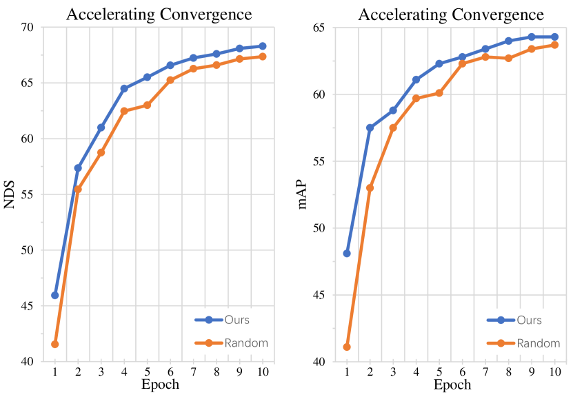
Figure 4: 3D object detection results on the nuScenes validation split. Our UniM²AE accerlerates the model convergence and ultimately improve the performance.

VI-B Additional Abalation Study

As shown in Figure 4, we compare the performance of detectors trained from scratch and pre-trained with our UniM²AE for 10 epochs. Our pre-training method significantly accelerates model convergence and finally stabilises it at a higher score when utilizing the entire dataset.

VI-C Pre-training Details

To fairly compare UniM²AE with the single-modal MAE methods (i.e. GreenMIM[33] and Voxel-MAE[34]), a consistent pre-training configuration shown in Table VII is adapted during the pre-training process. The detailed hyperparameters of MAE methods we used in this work are as follows.

TABLE VII: Pre-training Configuration.

Config	Value
optimizer	AdamW
base lr	5e-4
weight decay	0.001
batch size	32
lr schedule	cosine annealing
warmup iterations	1000
point cloud augmentation	random flip, resize
image augmentation	crop, resize, random flip
total epochs	200

VI-C1 UniM²AE hyperparameters

Generally, we employ the configuration of the encoder and decoder presented in GreenMIM[33] and Voxel-MAE[34] with adaptive modification to better suit multi-modal self-supervised pre-training. The image size is set to $\left[256,704\right]$ and the point cloud range is restrict in $\left[-50m,50m\right]$ for X-, Y- axes, $\left[-3m,5m\right]$ for Z-axes. At the same time, the volume grid shape is set to $\left[200,200,2\right]$. Specifically, to align multi-view images and LiDAR point cloud, only random flipping, resizing and cropping are used in the image augmentation, discarding other data augmentation methods originally applied to Masked Image Modeling.

For the Spatial Cross-Attention during the image to 3D volume projection, the number of deformable attention blocks is set to 6 with 256 hidden channels and $\mathcal{N}_{ref}$ is set to 4. In the Multi-modal Interaction Module (MMIM), we stack 3 deformable self-attention blocks comprising 8 heads in each block and the number of reference point is 4.

VI-C2 Baseline hyperparameters

In the experiments on data efficiency, we compare our UniM²AE with single-modal MAE methods, whose implementation follow their publicly released codes with minimal changes. Since GreenMIM[33] doesn’t employ Swin-T as their backbone while pre-training, we replaced their original Swin-B with Swin-T, and rigorously follow the other settings for pre-training. Additionally, for fair comparison, we use the same data augmentation in the camera branch of UniM²AE. For the Voxel-MAE[34], pre-training are done with intensity information in data efficiency experiment. The rest of the setup is the same as the Voxel-MAE.

VI-D Fine-tuning Details

TABLE VIII: Fine-tuning Configuration. Det denotes 3d object detection configuration. Seg denotes BEV map segmentation task configuration

Config	Value
		Det	Seg
point cloud range -x		[-54.0m, 54.0m]	[-51.2m, 51.2m]
point cloud range -y		[-54.0m, 54.0m]	[-51.2m, 51.2m]
point cloud range -x		[-3.0m, 5.0m]	[-3.0.m, 5.0m]
optimizer		AdamW	AdamW
base lr		1e-4	1e-4
weight decay		0.01	0.01
batch size		4	4

We evaluate our multi-modal self-supervised pre-training framework by fine-tuning two state-of-the-art detectors[14, 40], denoted as TransFusion-L-SST and BEVFusion-SST, whose LiDAR backbone is replaced by SST[43]. Detail configuration is presented in Table VIII.

In the 3D object detection task, we separately set the voxel size to $\left[0.5m,0.5m,8m\right]$ in the LiDAR-only method and $\left[0.5m,0.5m,4m\right]$ in the multi-modal method. During the pre-training we first transfer the weights of UniM²AE LiDAR encoder to TransFusion-L-SST and fintune it. We follow the TransFusion[40] training schedule and the results obtained by fine-tuning is denoted as UniM²AE-L. As for the multi-modal strategies, the weights of LiDAR encoder in UniM²AE-L and camera encoder pre-trained by UniM²AE are loaded to finetune the BEVFusion-SST following the BEVFusion[14] training schedule. Furthermore, we replace the fusion module in BEVFusion-SST by the pre-trained MMIM and get UniM²AE w/MMIM.

In the BEV map segmentation task, unlike the previous two-stage training schedule in the 3D object detection, we directly fine-tune the multi-modal BEVFusion-SST with $\left[0.2m,0.2m,4m\right]$ voxel size for 24 epochs and the camera-only BEVFusion[14] for 20 epochs, The changes regarding the backbone and fusion modules are the same as for the 3D detection task. For the camera-only detectors, all configuration is aligned with camera-only BEVFusion[14].

VI-E Visualization

In Figure 5, we provide examples of reconstruction visualizations. Our UniM²AE is able to reconstruct the masked LiDAR point clouds and multi-view images, accurately reflecting semantic and geometric understanding.

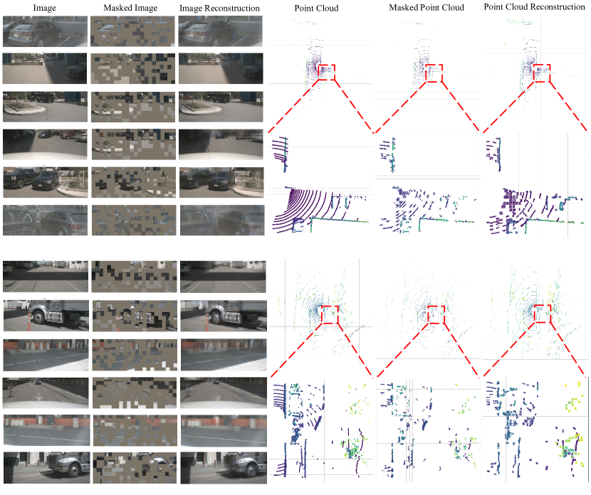
Figure 5: Visualization of reconstruction results. The reconstruction for two different scenes is presented, including 6 images and a point cloud. For ease of observation, we zoom in the point cloud at $\left[0m,15m\right]$ for X axes and $\left[-7.5m,7.5m\right]$ for Y axes.

VI-F Discussion about PiMAE

As mentioned in the main paper, [1] pre-trained PiMAE predominantly using indoor datasets like SUN RGB-D[56] and, in tandem, utilized Farthest Point Sampling (FPS) and K-Nearest Neighbors (KNN) in the point cloud branch. FPS is a sampling technique that select points far apart as possible from each other to provide a sparse and representative subset of the original set. Particularly, it first selects a point randomly, and then continuously chooses subsequent point that is the farthest from the already-selected points. KNN is a method used for classification and regression, but in the context of point clouds, it is often used to find the closest points to a given point. Given a point sampled by FPS, the KNN search would identify the k closest points to that point.

However the combination of FPS and KNN in PiMAE is not inherently suitable for outdoor datasets like nuScenes[9] in autonomous driving. The challenges arise due to the vast scale and spatial diversity of outdoor environments. On the indoor dataset SUN RGB-D[56], PiMAE[1] first uses FPS to filter 2048 points from about 20,000 points and then sends them into FPS and KNN to form 128 groups in order to save the GPU memory. However, in the outdoor dataset, the number of points in one scene often reach almost 200,000, and if the FPS is still employed to filter out only 2048 points, it might result in undersampling critical areas since FPS focuses on spreading out the sampled points. This can lead to missing important local structures, such as pedestrians, small obstacles or even the cars far away from the ego vehicle, which are essential for MAE methods to model the masked point clouds. Another option is to increase the number of output groups of FPS on the outdoor dataset. For example, we filter out 20,000 points from 200,000 points, send them into joint FPS+KNN operation and finally process the 1,000 output groups with the following point cloud encoder. Nevertheless since PiMAE[1] utilize multiple standard ViTs[57], whose computational complexity is $O(n^{2})$, in both encoder and decoder, the computational burden is still unacceptable even after downsampling 200 times.

References

- [1] A. Chen, K. Zhang, R. Zhang, Z. Wang, Y. Lu, Y. Guo, and S. Zhang, “Pimae: Point cloud and image interactive masked autoencoders for 3d object detection,” in Proceedings of the IEEE/CVF Conference on Computer Vision and Pattern Recognition, 2023, pp. 5291–5301.
- [2] Y. Pang, W. Wang, F. E. Tay, W. Liu, Y. Tian, and L. Yuan, “Masked autoencoders for point cloud self-supervised learning,” in European conference on computer vision. Springer, 2022, pp. 604–621.
- [3] X. Tian, H. Ran, Y. Wang, and H. Zhao, “Geomae: Masked geometric target prediction for self-supervised point cloud pre-training,” in Proceedings of the IEEE/CVF Conference on Computer Vision and Pattern Recognition, 2023, pp. 13 570–13 580.
- [4] H. Bao, L. Dong, S. Piao, and F. Wei, “Beit: Bert pre-training of image transformers,” arXiv preprint arXiv:2106.08254, 2021.
- [5] Z. Xie, Z. Zhang, Y. Cao, Y. Lin, J. Bao, Z. Yao, Q. Dai, and H. Hu, “Simmim: A simple framework for masked image modeling,” in Proceedings of the IEEE/CVF Conference on Computer Vision and Pattern Recognition, 2022, pp. 9653–9663.
- [6] K. He, X. Chen, S. Xie, Y. Li, P. Dollár, and R. Girshick, “Masked autoencoders are scalable vision learners,” in Proceedings of the IEEE/CVF conference on computer vision and pattern recognition, 2022, pp. 16 000–16 009.
- [7] R. Zhang, L. Wang, Y. Qiao, P. Gao, and H. Li, “Learning 3d representations from 2d pre-trained models via image-to-point masked autoencoders,” in Proceedings of the IEEE/CVF Conference on Computer Vision and Pattern Recognition, 2023, pp. 21 769–21 780.
- [8] Y. Zhou, P. Sun, Y. Zhang, D. Anguelov, J. Gao, T. Ouyang, J. Guo, J. Ngiam, and V. Vasudevan, “End-to-end multi-view fusion for 3d object detection in lidar point clouds,” in Conference on Robot Learning. PMLR, 2020, pp. 923–932.
- [9] H. Caesar, V. Bankiti, A. H. Lang, S. Vora, V. E. Liong, Q. Xu, A. Krishnan, Y. Pan, G. Baldan, and O. Beijbom, “nuscenes: A multimodal dataset for autonomous driving,” in Proceedings of the IEEE/CVF conference on computer vision and pattern recognition, 2020, pp. 11 621–11 631.
- [10] A. Radford, J. W. Kim, C. Hallacy, A. Ramesh, G. Goh, S. Agarwal, G. Sastry, A. Askell, P. Mishkin, J. Clark, et al., “Learning transferable visual models from natural language supervision,” in International conference on machine learning. PMLR, 2021, pp. 8748–8763.
- [11] L. Yao, R. Huang, L. Hou, G. Lu, M. Niu, H. Xu, X. Liang, Z. Li, X. Jiang, and C. Xu, “Filip: Fine-grained interactive language-image pre-training,” arXiv preprint arXiv:2111.07783, 2021.
- [12] R. Zhang, Z. Guo, W. Zhang, K. Li, X. Miao, B. Cui, Y. Qiao, P. Gao, and H. Li, “Pointclip: Point cloud understanding by clip,” in Proceedings of the IEEE/CVF Conference on Computer Vision and Pattern Recognition, 2022, pp. 8552–8562.
- [13] T. Huang, B. Dong, Y. Yang, X. Huang, R. W. Lau, W. Ouyang, and W. Zuo, “Clip2point: Transfer clip to point cloud classification with image-depth pre-training,” arXiv preprint arXiv:2210.01055, 2022.
- [14] Z. Liu, H. Tang, A. Amini, X. Yang, H. Mao, D. L. Rus, and S. Han, “Bevfusion: Multi-task multi-sensor fusion with unified bird’s-eye view representation,” in 2023 IEEE International Conference on Robotics and Automation (ICRA). IEEE, 2023, pp. 2774–2781.
- [15] T. Liang, H. Xie, K. Yu, Z. Xia, Z. Lin, Y. Wang, T. Tang, B. Wang, and Z. Tang, “Bevfusion: A simple and robust lidar-camera fusion framework,” Advances in Neural Information Processing Systems, vol. 35, pp. 10 421–10 434, 2022.
- [16] X. Yu, L. Tang, Y. Rao, T. Huang, J. Zhou, and J. Lu, “Point-bert: Pre-training 3d point cloud transformers with masked point modeling,” in Proceedings of the IEEE/CVF Conference on Computer Vision and Pattern Recognition, 2022, pp. 19 313–19 322.
- [17] H. Liu, M. Cai, and Y. J. Lee, “Masked discrimination for self-supervised learning on point clouds,” in European Conference on Computer Vision. Springer, 2022, pp. 657–675.
- [18] C. Min, D. Zhao, L. Xiao, Y. Nie, and B. Dai, “Voxel-mae: Masked autoencoders for pre-training large-scale point clouds,” arXiv preprint arXiv:2206.09900, 2022.
- [19] R. Xu, T. Wang, W. Zhang, R. Chen, J. Cao, J. Pang, and D. Lin, “Mv-jar: Masked voxel jigsaw and reconstruction for lidar-based self-supervised pre-training,” in Proceedings of the IEEE/CVF Conference on Computer Vision and Pattern Recognition, 2023, pp. 13 445–13 454.
- [20] H. Yang, T. He, J. Liu, H. Chen, B. Wu, B. Lin, X. He, and W. Ouyang, “Gd-mae: generative decoder for mae pre-training on lidar point clouds,” in Proceedings of the IEEE/CVF Conference on Computer Vision and Pattern Recognition, 2023, pp. 9403–9414.
- [21] A. Boulch, C. Sautier, B. Michele, G. Puy, and R. Marlet, “Also: Automotive lidar self-supervision by occupancy estimation,” in Proceedings of the IEEE/CVF Conference on Computer Vision and Pattern Recognition, 2023, pp. 13 455–13 465.
- [22] X. Chen, H. Ma, J. Wan, B. Li, and T. Xia, “Multi-view 3d object detection network for autonomous driving,” in Proceedings of the IEEE conference on Computer Vision and Pattern Recognition, 2017, pp. 1907–1915.
- [23] R. Nabati and H. Qi, “Centerfusion: Center-based radar and camera fusion for 3d object detection,” in Proceedings of the IEEE/CVF Winter Conference on Applications of Computer Vision, 2021, pp. 1527–1536.
- [24] X. Chen, T. Zhang, Y. Wang, Y. Wang, and H. Zhao, “Futr3d: A unified sensor fusion framework for 3d detection,” in Proceedings of the IEEE/CVF Conference on Computer Vision and Pattern Recognition, 2023, pp. 172–181.
- [25] S. Vora, A. H. Lang, B. Helou, and O. Beijbom, “Pointpainting: Sequential fusion for 3d object detection,” in Proceedings of the IEEE/CVF conference on computer vision and pattern recognition, 2020, pp. 4604–4612.
- [26] C. Wang, C. Ma, M. Zhu, and X. Yang, “Pointaugmenting: Cross-modal augmentation for 3d object detection,” in Proceedings of the IEEE/CVF Conference on Computer Vision and Pattern Recognition, 2021, pp. 11 794–11 803.
- [27] T. Yin, X. Zhou, and P. Krähenbühl, “Multimodal virtual point 3d detection,” Advances in Neural Information Processing Systems, vol. 34, pp. 16 494–16 507, 2021.
- [28] M. Liang, B. Yang, S. Wang, and R. Urtasun, “Deep continuous fusion for multi-sensor 3d object detection,” in Proceedings of the European conference on computer vision (ECCV), 2018, pp. 641–656.
- [29] Y. Li, A. W. Yu, T. Meng, B. Caine, J. Ngiam, D. Peng, J. Shen, Y. Lu, D. Zhou, Q. V. Le, et al., “Deepfusion: Lidar-camera deep fusion for multi-modal 3d object detection,” in Proceedings of the IEEE/CVF Conference on Computer Vision and Pattern Recognition, 2022, pp. 17 182–17 191.
- [30] Y. Wei, L. Zhao, W. Zheng, Z. Zhu, J. Zhou, and J. Lu, “Surroundocc: Multi-camera 3d occupancy prediction for autonomous driving,” arXiv preprint arXiv:2303.09551, 2023.
- [31] Z. Li, W. Wang, H. Li, E. Xie, C. Sima, T. Lu, Y. Qiao, and J. Dai, “Bevformer: Learning bird’s-eye-view representation from multi-camera images via spatiotemporal transformers,” in European conference on computer vision. Springer, 2022, pp. 1–18.
- [32] X. Zhu, W. Su, L. Lu, B. Li, X. Wang, and J. Dai, “Deformable detr: Deformable transformers for end-to-end object detection,” arXiv preprint arXiv:2010.04159, 2020.
- [33] L. Huang, S. You, M. Zheng, F. Wang, C. Qian, and T. Yamasaki, “Green hierarchical vision transformer for masked image modeling,” Advances in Neural Information Processing Systems, vol. 35, pp. 19 997–20 010, 2022.
- [34] G. Hess, J. Jaxing, E. Svensson, D. Hagerman, C. Petersson, and L. Svensson, “Masked autoencoder for self-supervised pre-training on lidar point clouds,” in Proceedings of the IEEE/CVF Winter Conference on Applications of Computer Vision, 2023, pp. 350–359.
- [35] H. Fan, H. Su, and L. J. Guibas, “A point set generation network for 3d object reconstruction from a single image,” in Proceedings of the IEEE conference on computer vision and pattern recognition, 2017, pp. 605–613.
- [36] J. Huang, G. Huang, Z. Zhu, Y. Ye, and D. Du, “Bevdet: High-performance multi-camera 3d object detection in bird-eye-view,” arXiv preprint arXiv:2112.11790, 2021.
- [37] Y. Liu, J. Yan, F. Jia, S. Li, A. Gao, T. Wang, X. Zhang, and J. Sun, “Petrv2: A unified framework for 3d perception from multi-camera images,” arXiv preprint arXiv:2206.01256, 2022.
- [38] T. Yin, X. Zhou, and P. Krahenbuhl, “Center-based 3d object detection and tracking,” in Proceedings of the IEEE/CVF conference on computer vision and pattern recognition, 2021, pp. 11 784–11 793.
- [39] Y. Chen, J. Liu, X. Zhang, X. Qi, and J. Jia, “Largekernel3d: Scaling up kernels in 3d sparse cnns,” in Proceedings of the IEEE/CVF Conference on Computer Vision and Pattern Recognition, 2023, pp. 13 488–13 498.
- [40] X. Bai, Z. Hu, X. Zhu, Q. Huang, Y. Chen, H. Fu, and C.-L. Tai, “Transfusion: Robust lidar-camera fusion for 3d object detection with transformers,” in Proceedings of the IEEE/CVF conference on computer vision and pattern recognition, 2022, pp. 1090–1099.
- [41] Y. Chen, Y. Li, X. Zhang, J. Sun, and J. Jia, “Focal sparse convolutional networks for 3d object detection,” in Proceedings of the IEEE/CVF Conference on Computer Vision and Pattern Recognition, 2022, pp. 5428–5437.
- [42] Y. Jiao, Z. Jie, S. Chen, J. Chen, L. Ma, and Y.-G. Jiang, “Msmdfusion: Fusing lidar and camera at multiple scales with multi-depth seeds for 3d object detection,” in Proceedings of the IEEE/CVF Conference on Computer Vision and Pattern Recognition, 2023, pp. 21 643–21 652.
- [43] L. Fan, Z. Pang, T. Zhang, Y.-X. Wang, H. Zhao, F. Wang, N. Wang, and Z. Zhang, “Embracing single stride 3d object detector with sparse transformer,” in Proceedings of the IEEE/CVF conference on computer vision and pattern recognition, 2022, pp. 8458–8468.
- [44] Z. Liu, Y. Lin, Y. Cao, H. Hu, Y. Wei, Z. Zhang, S. Lin, and B. Guo, “Swin transformer: Hierarchical vision transformer using shifted windows,” in Proceedings of the IEEE/CVF international conference on computer vision, 2021, pp. 10 012–10 022.
- [45] B. Zhou and P. Krähenbühl, “Cross-view transformers for real-time map-view semantic segmentation,” in Proceedings of the IEEE/CVF conference on computer vision and pattern recognition, 2022, pp. 13 760–13 769.
- [46] T. Roddick, A. Kendall, and R. Cipolla, “Orthographic feature transform for monocular 3d object detection,” arXiv preprint arXiv:1811.08188, 2018.
- [47] J. Philion and S. Fidler, “Lift, splat, shoot: Encoding images from arbitrary camera rigs by implicitly unprojecting to 3d,” in Computer Vision–ECCV 2020: 16th European Conference, Glasgow, UK, August 23–28, 2020, Proceedings, Part XIV 16. Springer, 2020, pp. 194–210.
- [48] E. Xie, Z. Yu, D. Zhou, J. Philion, A. Anandkumar, S. Fidler, P. Luo, and J. M. Alvarez, “M2bev: Multi-camera joint 3d detection and segmentation with unified birds-eye view representation,” arXiv preprint arXiv:2204.05088, 2022.
- [49] A. H. Lang, S. Vora, H. Caesar, L. Zhou, J. Yang, and O. Beijbom, “Pointpillars: Fast encoders for object detection from point clouds,” in Proceedings of the IEEE/CVF conference on computer vision and pattern recognition, 2019, pp. 12 697–12 705.
- [50] S. Borse, M. Klingner, V. R. Kumar, H. Cai, A. Almuzairee, S. Yogamani, and F. Porikli, “X-align: Cross-modal cross-view alignment for bird’s-eye-view segmentation,” in Proceedings of the IEEE/CVF Winter Conference on Applications of Computer Vision, 2023, pp. 3287–3297.
- [51] Y. Yan, Y. Mao, and B. Li, “Second: Sparsely embedded convolutional detection,” Sensors, vol. 18, no. 10, p. 3337, 2018.
- [52] Y. Chen, J. Liu, X. Zhang, X. Qi, and J. Jia, “Voxelnext: Fully sparse voxelnet for 3d object detection and tracking,” in Proceedings of the IEEE/CVF Conference on Computer Vision and Pattern Recognition, 2023, pp. 21 674–21 683.
- [53] Y. Li, Y. Chen, X. Qi, Z. Li, J. Sun, and J. Jia, “Unifying voxel-based representation with transformer for 3d object detection,” Advances in Neural Information Processing Systems, vol. 35, pp. 18 442–18 455, 2022.
- [54] Y. Li, X. Qi, Y. Chen, L. Wang, Z. Li, J. Sun, and J. Jia, “Voxel field fusion for 3d object detection,” in Proceedings of the IEEE/CVF Conference on Computer Vision and Pattern Recognition, 2022, pp. 1120–1129.
- [55] H. Wang, C. Shi, S. Shi, M. Lei, S. Wang, D. He, B. Schiele, and L. Wang, “Dsvt: Dynamic sparse voxel transformer with rotated sets,” in Proceedings of the IEEE/CVF Conference on Computer Vision and Pattern Recognition, 2023, pp. 13 520–13 529.
- [56] S. Song, S. P. Lichtenberg, and J. Xiao, “Sun rgb-d: A rgb-d scene understanding benchmark suite,” in Proceedings of the IEEE conference on computer vision and pattern recognition, 2015, pp. 567–576.
- [57] A. Dosovitskiy, L. Beyer, A. Kolesnikov, D. Weissenborn, X. Zhai, T. Unterthiner, M. Dehghani, M. Minderer, G. Heigold, S. Gelly, et al., “An image is worth 16x16 words: Transformers for image recognition at scale,” arXiv preprint arXiv:2010.11929, 2020.