Further investigation of dilepton-based center-of-mass energy measurements at e⁺e^- colliders

Abstract

Methods for measuring the absolute center-of-mass energy using dileptons from e⁺e^- collision events are further developed with an emphasis on accelerator, detector, and physics limitations. We discuss two main estimators, the lepton momentum-based center-of-mass energy estimator, $\sqrt{s}_{p}$, discussed previously, and new estimators for the electron and positron colliding beam energies, denoted $E^{\text{C}}_{-}$ and $E^{\text{C}}_{+}$. In this work we focus on the underlying limitations from beam energy spread, detector resolution, and the modeling of higher-order QED radiative corrections associated with photon emissions originating from initial-state-radiation (ISR), final-state-radiation (FSR), and their interference. We study the consequent implications for the potential of these methods at center-of-mass energies ranging from 90 GeV to 1 TeV relevant to a number of potential accelerator realizations in the context of measurements of masses of the Z, W, H, top quark, and new particles. The statistical importance of the Bhabha channel for Higgs factories is noted. Additional extensive work on improving the modeling of the luminosity spectrum including the use of copulas is also reported.

Submitted to the Proceedings of the International Workshop on
Future Linear Colliders (LCWS 2023)

1 Introduction

Recent work on measuring the absolute center-of-mass energy using dileptons (specifically dimuons) from collision events at future $\mathrm{e}^{+}\mathrm{e}^{-}$ colliders was reported in [1]. For ILC beam conditions at $\sqrt{s}=250$ GeV and using full simulation of the ILD detector concept, it was shown that a statistical precision of 2.1 ppm on the center-of-mass energy scale could be achieved with a 2.0 $\mathrm{ab}^{-1}$ unpolarized data-set with the dimuon channel alone using the $\sqrt{s}_{p}$ center-of-mass energy estimator based on the measurement of the muon momenta. In this work, we report on a number of new developments that advance our understanding of the utility and potential of this method.

2 Colliding Beam Energies using $\mathrm{e}^{+}\mathrm{e}^{-}\to\mu_{1}^{+}\mu_{2}^{-}(\gamma)$

One can infer knowledge of the $\mathrm{e}^{-}$ and $\mathrm{e}^{+}$ beam energies of the actual collision from the muons alone under the assumption of one collinear but undetected ISR photon. The energy and $z$-direction longitudinal momentum ($E,p_{z}$) conservation equations in the lab frame are

$$E_{-}+E_{+} =E_{1}+E_{2}+|p_{\gamma}^{z}|/\cos(\alpha/2)\>\>,$$ (1)

$$(E_{-}-E_{+})\cos(\alpha/2) =p_{1}^{z}+p_{2}^{z}+p_{\gamma}^{z}\>\>,$$ (2)

where $E_{-}$ and $E_{+}$ are the energies of the colliding beam particles in the lab frame, with crossing-angle, $\alpha$, ($E_{1},p_{1}^{z}$) and ($E_{2},p_{2}^{z}$) are the energies and $z$-direction longitudinal momenta of the anti-muon and muon respectively, and $p_{\gamma}^{z}$, is the $z$-component of the momentum of the collinear (with one of the beams) undetected ISR photon.

These can be solved for $E_{-}$ and $E_{+}$, leading to:

$$E_{-} =\frac{1}{2}\left[(E_{1}+E_{2})+\frac{(p_{1}^{z}+p_{2}^{z})}{\cos{(\alpha/2)}}\right]+\frac{(|p_{\gamma}^{z}|+p_{\gamma}^{z})}{2\cos(\alpha/2)}\>\>,$$ (3)

$$E_{+} =\frac{1}{2}\left[(E_{1}+E_{2})-\frac{(p_{1}^{z}+p_{2}^{z})}{\cos{(\alpha/2)}}\right]+\frac{(|p_{\gamma}^{z}|-p_{\gamma}^{z})}{2\cos(\alpha/2)}\>\>,$$ (4)

where of course one has assumed the unknowable knowledge of the actual ISR photon momentum. Instead, dropping the ISR photon terms in each equation leads to the following estimators,

$$E^{\text{C}}_{-} =\frac{1}{2}\left[(E_{1}+E_{2})+\frac{(p_{1}^{z}+p_{2}^{z})}{\cos{(\alpha/2)}}\right]\>\>,$$ (5)

$$E^{\text{C}}_{+} =\frac{1}{2}\left[(E_{1}+E_{2})-\frac{(p_{1}^{z}+p_{2}^{z})}{\cos{(\alpha/2)}}\right]\>\>,$$ (6)

which rely simply on the muon measurements and neglect the undetected ISR photon. Obviously, the errors on these estimates, $\Delta E^{\text{C}}_{\pm}$, that are caused by dropping the ISR photon terms are:

$$\Delta E^{\text{C}}_{-} =E^{\text{C}}_{-}-E_{-}=-\frac{(|p_{\gamma}^{z}|+p_{\gamma}^{z})}{2\cos(\alpha/2)}\>\>,$$ (7)

$$\Delta E^{\text{C}}_{+} =E^{\text{C}}_{+}-E_{+}=-\frac{(|p_{\gamma}^{z}|-p_{\gamma}^{z})}{2\cos(\alpha/2)}\>\>.$$ (8)

The consequence of the ISR photon induced error on $E^{\text{C}}_{\pm}$ depends on which beam emitted the photon as characterized by the sign of the ISR photon’s longitudinal momentum:

$$(\Delta E^{\text{C}}_{-},\Delta E^{\text{C}}_{+}) =\begin{cases}(0,\>-E_{\gamma})&p_{\gamma}^{z}<0\\ (-E_{\gamma},\>0)&p_{\gamma}^{z}>0\>\>.\end{cases}$$ (9)

When the ISR photon is emitted from the positron beam ($p_{\gamma}^{z}<0$), $E^{\text{C}}_{-}$ is exact under the assumption of one collinear undetected ISR photon, but $E^{\text{C}}_{+}$ can be very wrong (underestimated by the photon energy, $E_{\gamma}=|p_{\gamma}^{z}|/\cos{(\alpha/2)}$). Conversely, when the ISR photon is emitted from the electron beam ($p_{\gamma}^{z}>0$), $E^{\text{C}}_{+}$ is exact, but $E^{\text{C}}_{-}$ can be very wrong. Thus for each event this method allows exact reconstruction of one of the colliding beam particle energies under the one collinear ISR photon assumption. Identifying, with certainty, which one is exact on an event-by-event basis is not feasible, but the method does provide statistical information related to the distribution of the colliding beam particle energies. Furthermore, we should emphasize that the obtained estimate, which corresponds to the actual colliding beam energy in the lab frame, is sensitive to the combined effect of the colliding particle’s energy deviation from nominal arising from both the beam energy spread fluctuation and the often present beamstrahlung-induced energy loss.

Figure 1 illustrates these distributions at the WHIZARD [2, 3] generator level for ILC at $\sqrt{s}=250$ GeV with super-imposed fits corresponding to the convolution with a single Gaussian of an admixture of a beta distribution and a delta function as described in A.1. The fitted Gaussian resolution parameter, $\sigma$, is very similar to the intrinsic expectation from beam energy spread alone of 0.190% ($\mathrm{e}^{-}$) and 0.152% ($\mathrm{e}^{+}$) indicating as expected that the peak regions of these distributions retain significant information relevant to characterizing the initial beam parameters and distributions.

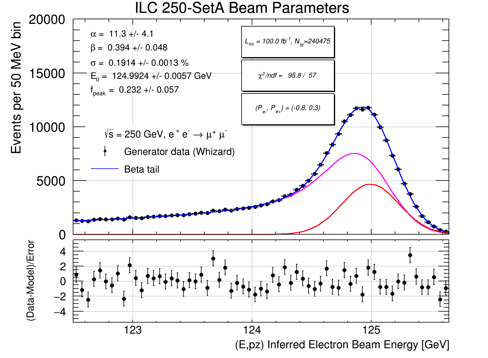
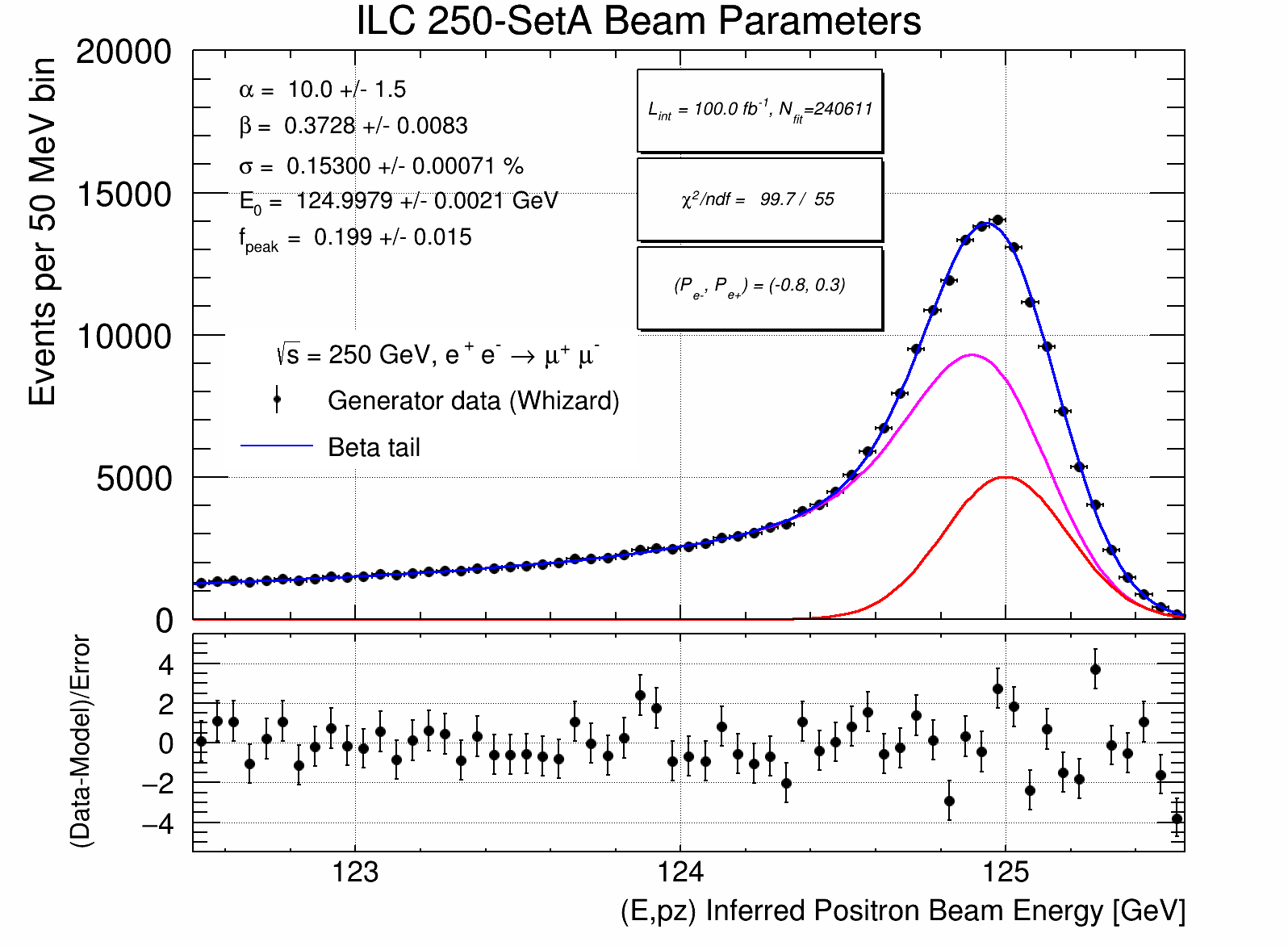
Figure 1: Distribution of the inferred colliding electron beam energy, $E^{\mathrm{C}}_{-}$ (top), and the inferred colliding positron beam energy, $E^{\mathrm{C}}_{+}$ (bottom), at generator level for $\mathrm{e}^{+}\mathrm{e}^{-}\rightarrow\mu^{+}\mu^{-}(\gamma)$ events with super-imposed 5-parameter fits. The simulation includes the effects of beam energy spread, beamstrahlung, and radiative corrections as included in the WHIZARD-based iLCSoft samples.

Observable	$\sqrt{s}$	$E_{\mathrm{b}}^{-}$	$E_{\mathrm{b}}^{+}$	$2\sqrt{\hat{E}_{\mathrm{b}}^{-}\hat{E}_{\mathrm{b}}^{+}}\cos(\alpha/2)$
WHIZARD generator level	3.8	3.2	2.6	2.1
Generator level estimator	5.8	6.4	5.3	4.1
Detector level estimator	7.8	12.5	12.2	8.7

Table 1: Statistical precision estimates on the absolute scale of the center-of-mass energy, $\sqrt{s}$, and the electron and positron beam energies ($E_{\mathrm{b}}^{-}$ and $E_{\mathrm{b}}^{+}$) in parts per million (ppm) for 100 $\mathrm{fb}^{-1}$ of $\mathrm{e}^{+}\mathrm{e}^{-}\rightarrow\mu^{+}\mu^{-}(\gamma)$ events with $P(\mathrm{e}^{-})=-0.8$ and $P(\mathrm{e}^{+})=+0.3$ at $\sqrt{s}=250$ GeV for ILC. The statistical energy scale uncertainties are the result of fits to the relevant distributions with the shape parameters fixed to their best-fit values, but the one scale-related location parameter floating. The $\sqrt{s}_{p}$ estimator is used for the $\sqrt{s}$ estimate, and the ($E,p_{z}$)-inferred colliding beam energy estimators are used for $E_{\mathrm{b}}^{-}$ and $E_{\mathrm{b}}^{+}$. The WHIZARD generator level values represent fits to the true distributions of $\sqrt{s}$, $E_{\mathrm{b}}^{-}$, and $E_{\mathrm{b}}^{+}$ differing only from the pure luminosity spectrum equivalent by the convolution with the cross-section. The generator level estimator includes effects from ISR and FSR that invalidate the assumptions. Detector level estimates use ILD full simulation with dimuons classed in the gold, silver, and bronze $\sqrt{s}_{p}$ resolution categories and includes the effects of acceptance, efficiency, and resolution. The last column gives the propagated uncertainty on the center-of-mass energy scale using the single beam energy scale estimates neglecting potential correlations.

Table 1 shows a comparison of the statistical precisions for $\sqrt{s}$ and the individual beam energies using the $\sqrt{s}_{p}$, $E^{\mathrm{C}}_{-}$, and $E^{\mathrm{C}}_{+}$ observables at generator and detector level and a corresponding estimate of the center-of-mass energy from the individual beam energy estimates. There are two main intrinsic effects affecting the WHIZARD generator level estimates for $\sqrt{s},E_{\mathrm{b}}^{-},E_{\mathrm{b}}^{+}$: the different fractional standard deviations associated with pure beam energy spread (0.12%, 0.19%, 0.15%) and the different probabilities, and therefore purity for negligible beamstrahlung induced energy loss. Using the same characterization as in Section 4, 25.20% of luminosity spectrum events are in the joint peak region, while 48.01% are in the peak regions of each beam. The statistical precision on $\sqrt{s}$ using $\sqrt{s}_{p}$ is degraded first by physics effects (the assumptions of the $\sqrt{s}_{p}$ method), and then additionally by detector resolution. A similar picture is at play for the $E^{\mathrm{C}}_{-}$ and $E^{\mathrm{C}}_{+}$ observables but there is a larger degradation than for $\sqrt{s}$. Some of this is the effective factor of two loss in beam particle numbers associated with the hemisphere ambiguity, but the generator estimator to detector estimator degradation is surprisingly big, and deserves more study.

3 Beam Energy Spread

The beam energy spread is a fundamental limitation on how well one can measure the center-of-mass energy. It affects the “luminosity spectrum” and induces a variable longitudinal boost. The fractional energy spread, for the energies of each beam and of the center-of-mass assuming Gaussian uncorrelated beams, is illustrated in Fig. 2 for ILC and FCC-ee. As one can see the fractional energy spread decreases with center-of-mass energy for linear colliders and increases with center-of-mass energy for circular colliders. Note beamstrahlung effects are not included in the figure for ILC, but they are included for FCC-ee where the multi-orbit effect results in effectively an increased pre-collision energy spread. The ILC is described in [4] with an accelerator configuration for the Z discussed originally in detail in [5]; the same considerations are used for the $\sqrt{s}=161$ GeV parameters.

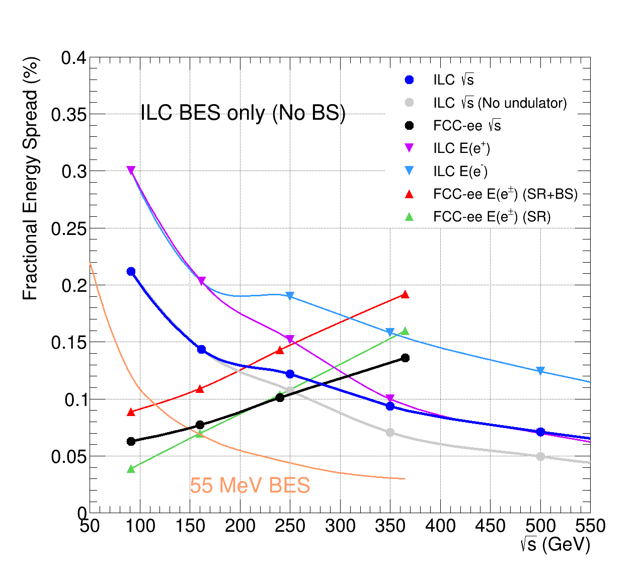
Figure 2: Fractional energy spread on the center-of-mass energy for ILC (dark blue), FCC-ee (black) and ILC with no undulator (gray). Also shown are the spreads for the individual beam energies. For ILC the electron energy spread (light blue) is degraded additionally compared to the positron (violet) by passage through the undulator used for positron production. For FCC-ee the total beam energy spread is shown in red while the synchrotron radiation component is shown in green. The orange curve with a beam energy spread of 55 MeV delimits the region to the lower left where resonant depolarization based beam energy measurement may be feasible.

One sees that the center-of-mass energy spread varies from 0.21% at $\sqrt{s}=91$ GeV to 0.07% at $\sqrt{s}=500$ GeV for ILC, while it varies from 0.06% at $\sqrt{s}=91$ GeV to 0.14% at $\sqrt{s}=365$ GeV for FCC-ee, and is 0.10–0.12% in the $\sqrt{s}=250$ GeV region for both. This sets corresponding targets for momentum resolution.

4 Improved/More Versatile Modeling of the Luminosity Spectrum

In our previous work [1] based on the standard ILC generator files we noted some deficiencies in the smoothness of the simulated beam-related distributions (see also Fig. 1). This likely arises from the combined behavior of the specific implementation of the Guinea-PIG based beam simulation [6] modeling of the luminosity spectrum and the numerical sampling from this luminosity spectrum using the CIRCE2 interface in the WHIZARD event generator. For an introduction and in-depth discussion of luminosity spectrum issues see [7]. We identified two specific modeling limitations that play at least a partial role. Firstly, the input beam energy distributions were truncated at $\pm 3.0$ standard deviations, and secondly, the input beam energy distributions were only sampled from a limited set of the same 80,000 beam particles (separately for $\mathrm{e}^{-}$ and $\mathrm{e}^{+}$) in each Guinea-PIG run.

The CIRCE2 implementation uses a purely numerical grid-based model for interfacing simulated luminosity spectra with event generators. However we have been encouraged by the relative simplicity of the ILC luminosity spectra at $\sqrt{s}=250$ GeV and have pursued a parametric approach to luminosity spectrum modeling similar to CIRCE1 [8]. In the past the observation that the electron and positron energy distributions are not independent led to arguably a premature abandonment of the parametric approach, which has the potential to be more versatile, accurate, and reproducible. To address these issues in a manner that promised to be expedient for the dilepton studies, and is likely of wider utility, we have made progress in a number of directions:

1. Simplifying the use of Guinea-PIG for beam simulations targeted at physics and detector studies by avoiding the use of input beam files and deferring the simulation of beam energy spread to a second step. In this way the Guinea-PIG output consists only of the luminosity spectrum with beamstrahlung effects. To simplify the simulations the force_symmetric setting is turned on (assumes symmetric charge distributions). It is also straightforward to implement different (Gaussian) beam energy spread settings. However it is not clear how to include explicit E-$z$ beam correlations, where $z$ is the co-moving longitudinal coordinate of the bunch.

   This setup has been used in the development of the GP2X framework reported in [9] where events from Guinea-PIG runs are used for luminosity spectrum modeling and are mixed with events from physics event generators.

2. Parametrization of these pure beamstrahlung luminosity spectra using a model with separate two-component mixtures of beta distributions for the “Body” region and the “Arms” regions together with a delta function “Peak” region component. This is inspired by André Sailer’s “CoPa” parametrization [10]. The regions in the scaled 2-d energy distribution of the electron and positron, ($x_{-},x_{+}$), where $x_{-}=E_{\mathrm{b}}^{-}/E_{\mathrm{b}}^{\text{nom}}$ and $x_{+}=E_{\mathrm{b}}^{-}/E_{\mathrm{b}}^{\text{nom}}$, are defined by whether the fractional energy loss of each beam exceeds 2 ppm as illustrated in Fig. 3.

3. Use of copulas to parametrize the dependence issues in the pure beamstrahlung luminosity spectra for the Body events where both beams experience significant energy loss from beamstrahlung.

4. Developing a simple stochastic model for generating luminosity spectrum events including dependence effects (ie. electron/positron energy correlations) and beam energy spread.

For item (2), we have used 2M Guinea-PIG simulated events for the ILC $\sqrt{s}=250$ GeV configuration with no beam energy spread using the Guinea-PIG++ implementation [11]. We used 20 independent runs of 100,000 events with 500,000 macroparticles in each run to better avoid the noted non-stochastic issues. These simulated events are also used in the GP2X study.

With the region definitions of Fig 3, 25.20% of events lie in the Peak region, 45.62% in the Arms regions, and the remaining 29.18% in the Body region. We have fitted the Guinea-PIG distributions of $x_{\pm}$ for the events in the Body region (two entries per Body event) and the $x_{\pm}$ distribution using $x_{-}$ for the Arm$-$ region and $x_{+}$ for the Arm$+$ region (one entry per Arm event). The fits are done as a function of the transformed variable, $t\equiv(1-x)^{1/\eta}$, with $\eta=4$. The resulting fits with a double beta tail model described in A.2 are summarized in Table 2. They are fairly reasonable.

Figure 3: The regions in the scaled energies of the electron and positron beam, $x_{-}$ and $x_{+}$, respectively. For the standard tests, the regions were defined using $1-x_{\pm}=2\times 10^{-6}$, which is three orders of magnitude smaller than the the typical beam energy spread of 0.17%.

Parameter	Body	Arms
$\alpha_{1}$	$13.61\pm 0.12$	$15.26\pm 0.21$
$\beta_{1}$	$0.3579\pm 0.0017$	$0.377\pm 0.016$
$\alpha_{2}$	$39.9\pm 7.4$	$31.5\pm 1.6$
$\beta_{2}$	$0.611\pm 0.066$	$0.328\pm 0.016$
$f_{1}$	$0.939\pm 0.017$	$0.674\pm 0.037$
$\chi^{2}/\nu$	123.0/68	79.6/68
$p_{\text{region}}$(%)	$29.179\pm 0.032$	$45.619\pm 0.035$

Table 2: Parameter values for the 5-parameter double beta function fits to the Body and Arms regions for ILC at $\sqrt{s}=250$ GeV. Also listed are the multinomial observed probabilities (no fit) for falling in each region.

For the 29.2% of events that lie in the Body region we also need to take care of modeling the dependence structure in the Body region’s ($x_{-},x_{+}$) bivariate distribution. Some dependence is expected because of the finite bunch length as interactions occurring from head-head collisions tend to have less energy loss compared with those from tail-tail collisions which tend to have more energy loss.

Instead of attempting to fit the bivariate probability distribution, $p(x_{-},x_{+})$, in its entirety, we will use the copula approach to factor the modeling problem into two more manageable pieces. The first piece is the modeling of the marginal distributions and the second is the determination of the dependence structure using copulas. The marginal distributions were already found above. Thus, we already have a parametrization from the performed fit for the $x_{-}$ and $x_{+}$ marginal distributions, $p(x_{-})$ and $p(x_{+})$, (assumed to be equal here) where,

$$p(x_{-})=\int p(x_{-},x_{+})dx_{+}=\int p(x_{-},x_{+})dx_{-}=p(x_{+}).$$ (10)

We do not explicitly know $p(x_{-},x_{+})$ yet, and we will not need to directly find it.

Next we tackle the issue of dependence modeling using copulas. The techniques are applied frequently in quantitative finance but are far less common in the physical sciences. The monographs of Nelsen [12] and Joe [13] and references therein are comprehensive guides to the rich literature. Before delving too much into copulas let us first establish that there is some appreciable dependence to model in the problem at hand. There are a variety of statistics that can be applied to the observed $(x_{-},x_{+})$ distribution. We have computed Blomqvist’s beta (medial correlation coefficient), Spearman’s rho (rank correlation coefficient), and Kendall’s tau (concordance based rank correlation coefficient) for Guinea-PIG runs with ILC accelerator conditions at 91, 161, and 250 GeV (again neglecting beam energy spread). These statistics should all be consistent with zero if there is no dependence, i.e. if the $x_{-}$ and $x_{+}$ variables are independent. Results are reported in Table 3 (see [13] for definitions) establishing clearly that for all center-of-mass energies, but especially for $\sqrt{s}=250$ GeV, that there is a significant, but relatively small, dependence present.

$\sqrt{s}$ (GeV)	$N$	$\beta_{B}$ (%)	$\rho_{S}$ (%)	$\tau_{K}$ (%)
91	185,589	$1.21\pm 0.23$	$1.59\pm 0.23$	$1.06\pm 0.15$
161	347,021	$1.70\pm 0.17$	$2.65\pm 0.17$	$1.77\pm 0.11$
250	583,584	$3.66\pm 0.13$	$5.41\pm 0.13$	$3.61\pm 0.09$

Table 3: Measured values of Blomqvist’s beta, Spearman’s rho, and Kendall’s tau dependence statistics in the Body region for Guinea-PIG ILC samples with 2M events at 91, 161, 250 GeV. The number of events in the Body region with the $1-x=2\times 10^{-6}$ separation definition is given in the second column.

So what is a copula? The copula of a random variable vector ($X_{-},X_{+}$) is defined as the joint cumulative distribution function of the random variable vector ($U_{-},U_{+}$),

$$C(u_{-},u_{+})=\text{Pr}[U_{-}\leq u_{-},U_{+}\leq u_{+}]\>\>,$$

where ($U_{-},U_{+}$) is related to ($X_{-},X_{+}$) via the cumulative distribution functions ($F_{-}$ and $F_{+}$) of the original univariate marginal distributions by

$$(U_{-},U_{+})=(F_{-}(X_{-}),F_{+}(X_{+}))\>\>,$$

and as usual,

$$F_{-}(x)=\text{Pr}[X_{-}\leq x]\>\>\text{and}\>\>F_{+}(x)=\text{Pr}[X_{+}\leq x]\>\>.$$

With this construction, the $C(u_{-},u_{+})$ copula’s univariate marginal distributions are both uniformly distributed on [0,1]. The copula provides the link between the marginal distributions of $x_{-}$ and $x_{+}$ and the joint distribution of $(x_{-},x_{+})$. Now we seek a copula model that fits adequately the dependence of the observed $(x_{-},x_{+})$ distribution. After some trial and error, we chose a 3-parameter mixture model of the 1-parameter Clayton and Ali-Mikhail-Haq (AMH) copulas,

$$C(u_{-},u_{+};\phi,\theta_{C},\theta_{AMH})=\cos^{2}{\phi}\>C_{1}(u_{-},u_{+};\theta_{C})+\sin^{2}{\phi}\>C_{2}(u_{-},u_{+};\theta_{AMH})\>\>.$$

Here the $\phi$ parameter is used to adjust the weight of each copula while respecting normalization and positivity requirements, the Clayton copula, defined for $0\leq\theta_{C}<\infty$, is

$$C_{1}(u_{-},u_{+};\theta_{C})=(u_{-}^{-\theta_{C}}+u_{+}^{-\theta_{C}}-1)^{-1/\theta_{C}}\>\>,$$

and the AMH copula, defined for $-1\leq\theta_{AMH}\leq 1$, is

$$C_{2}(u_{-},u_{+};\theta_{AMH})=\frac{u_{-}u_{+}}{1-\theta_{AMH}(1-u_{-})(1-u_{+})}\>\>.$$

We fitted this model to the 250 GeV Guinea-PIG ILC sample. The fit was done using a pseudo-likelihood fit to the simulated data cast as an empirical copula by maximizing,

$${\cal{L}}(\phi,\theta_{C},\theta_{AMH})=\prod_{i=1}^{N}c(U^{i}_{-},U^{i}_{+};\phi,\theta_{C},\theta_{AMH})\>\>.$$

Here $c$ is the corresponding probability density function obtained from differentiating the copula model. It is evaluated at points $(U^{i}_{-},U^{i}_{+})$ for each event, $i$, computed on the unit square using the ranks, $R^{-}_{i}$ and $R^{+}_{i}$ from 1 to $N$, of the observed $x_{-}$ and $x_{+}$ values, by defining $U^{i}_{-}=(R^{-}_{i}-0.5)/N$ and $U^{i}_{+}=(R^{+}_{i}-0.5)/N$. A rank of 1 corresponds to the lowest observed value for the corresponding $x_{\pm}$ variable. This leads to the sampled marginal distributions of the empirical copula being perfectly uniform (with no fluctuations) rather than just being distributed uniformly as required by the definition. The use of ranks makes the determination of the copula parameters independent of the modeling of the original univariate marginal distributions. The fit results with the obtained parameter values are shown in Table 4 and the data to model comparison is shown in Figure 5 using dependence deviations based on the functions denoted left and right tail concentration functions in [14], which are related to the probability content in the lower-left and upper-right square regions of the 2-d copula distribution, and defined as

$$L(z)=\text{Pr}(U_{-}<z,U_{+}<z)/z\>\>,$$

and

$$R(z)=\text{Pr}(U_{-}>z,U_{+}>z)/(1-z)\>\>.$$

If there is no dependence, one expects $L(z)=z$ and $R(z)=1-z$, and so the plotted variable is the deviation formed by subtracting the expected values under the independence hypothesis. One sees that the left tail (region of large energy loss in both beams) has a significant positive dependence and also the right tail (small energy loss in both beams) has a smaller positive dependence. The fitted model agrees well with the observed shape of the measured deviations from independence as a function of $z$.

$\sqrt{s}$ (GeV)	$\phi$ (rad)	$\theta_{C}$	$\theta_{AMH}$
250	$0.444\pm 0.070$	$0.0497\pm 0.0051$	$0.36\pm 0.10$

Table 4: Values for the copula parameters fitted to the Guinea-PIG ILC sample with 2M events at 250 GeV.

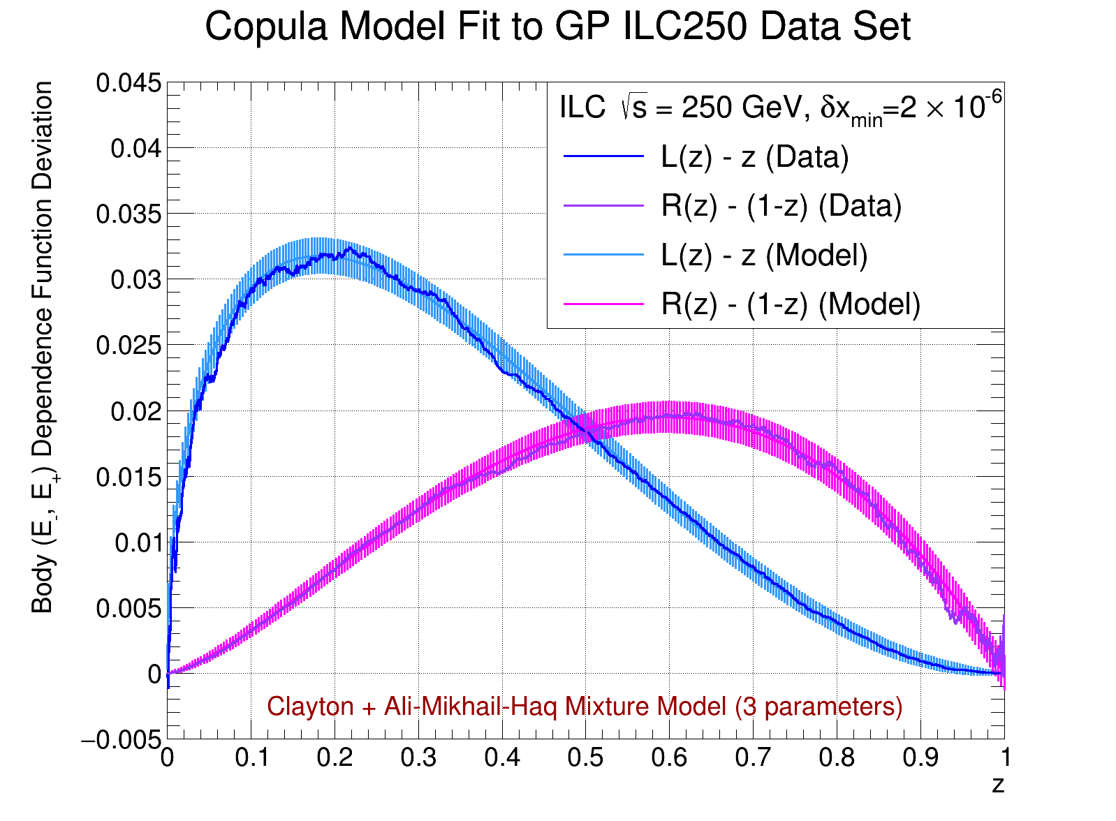
Figure 4: Comparison of the simulated data from Guinea-PIG for ILC at $\sqrt{s}=250$ GeV in the Body region to the predictions of the fitted model in terms of the dependence function deviations, $L(z)-z$ and $R(z)-(1-z)$, that should be zero for all $z$ in [0,1] for no dependence. The displayed uncertainties show the statistical uncertainties on the model prediction for the sample size of the simulated data ($N=583,584)$. Note given the use of cumulative distributions the bin-to-bin uncertainties are not independent.

A goodness-of-fit statistic was calculated using chi-squared with 10,000 cells each with dimension of $0.01\times 0.01$ on the unit square, and found $\chi^{2}/\nu=9488.4/9797$ where the calculated number of degrees of freedom, $\nu$, takes into account the three fit parameters and the 200 constraints implicit in the empirical copula construction. We also followed this up with more formal testing using a parametric bootstrap based on the Cramér–von Mises statistic ($S_{n}$) following the methodology of Appendix A in [15] and found a $p$-value of about 98% confirming the initial impression that the copula fit model fits well. As part of this bootstrap procedure we developed a stochastic implementation to generate events from the copula model.

We have also developed a stochastic implementation that generates events from the ($E_{-},E_{+}$) luminosity spectrum after beamstrahlung and beam energy spread. This uses the 10 parameters of the marginal distribution fits of Table 2, the two region probability parameters, two parameters for the Gaussian beam energy spread of each beam, two parameters for potential (small) changes in energy scale of each beam and the three copula parameters for Body events for a total of 17 parameters. The region (Peak, Arm$-$, Arm$+$, Body) is chosen by throwing a single uniform random number. Values of ($x_{-},x_{+}$) are generated according to the defined beamstrahlung-only model including the dependence structure for Body events and where beams with $1-x<2\times 10^{-6}$ are set to $x=1.0$ (Peak and Arms events). The ($E_{-},E_{+}$) distribution including Gaussian beam energy spread effects is then obtained by smearing and potentially shifting the ($x_{-},x_{+}$) values and scaling up to the nominal beam energy scale. It is also straightforward to set the copula part of the model to the independence copula where the bivariate distribution has no dependence. This parametric model should be relatively easy to adopt in physics event generators and we welcome collaboration to facilitate this.

5 Testing New Luminosity Spectrum Modeling

We generated 20 million events from the fitted copula model and 20 million events from a model with no copula (independence copula). The comparison of the center-of-mass energy in the luminosity spectrum is shown in Fig. 5. One sees some differences at the 1% level which we will see has some effect on the fitted parameters of the respective luminosity spectrum.

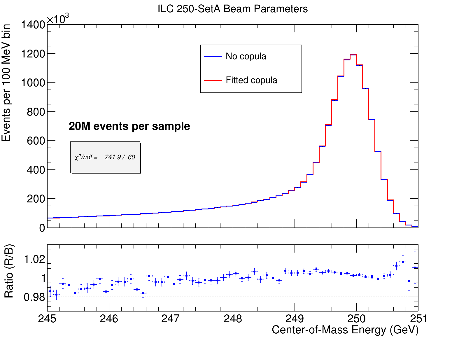
Figure 5: Distribution of center-of-mass energy for the two luminosity spectrum models. Twenty million events are sampled from each model with identically distributed marginal distributions. In the no copula model (blue), the electron and positron energy distributions in the Body part of the distribution are independent, while for the fitted copula model (red) they have a dependence according to the 3-parameter copula model fitted to the Guinea-PIG data. The lower panel shows the ratio of sampled observations for the fitted copula model to those from the no copula model.

Shown in Fig. 6 are fits to the luminosity spectrum for the no copula model (top panel) and the fitted copula model (bottom panel) using the 5-parameter Gaussian peak and convolved beta tail model described in A.1. One sees satisfactory fits despite the underlying model used in the event generation having 17 parameters. We believe this indicates that the beam energy spread is sufficiently large to smear out the fine details needed to model the pre beam energy spread distributions.

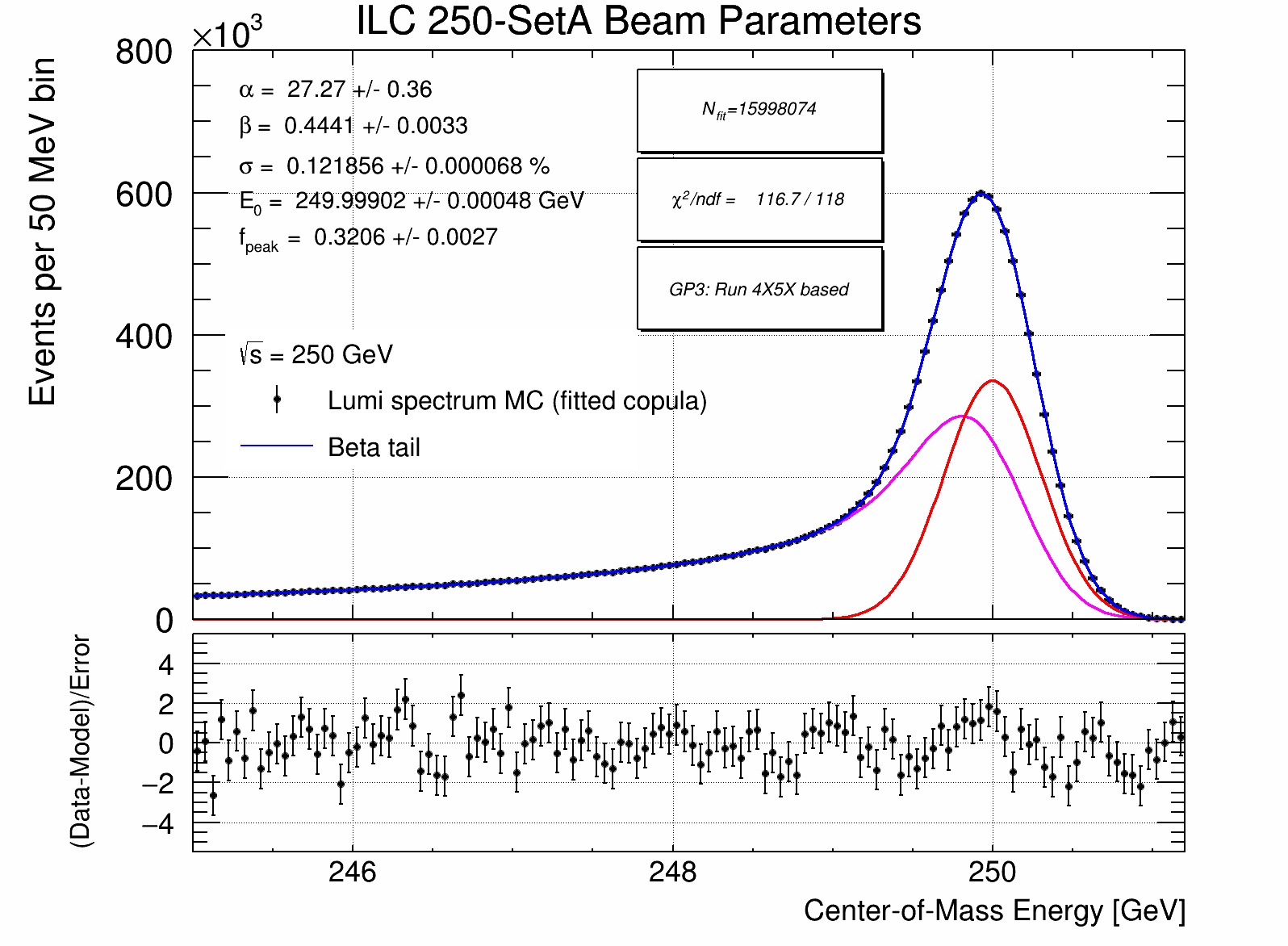
Figure 6: Fits to the center-of-mass energy distributions for the two luminosity spectrum models of Fig. 5.

Clearly the fitted parameters from these semi-empirical fits indicate subtle but likely significant differences. When each fit is repeated with all but the $E_{0}$ parameter fixed to the best fit values for their own data-sets, the fitted energy scale with no copula is found to be $5.0\pm 0.7$ ppm higher than that for the fitted copula data-set. Assessed another way, if the non-$E_{0}$ parameters of the fit to the fitted copula data-set are fixed and imposed on the fit to the no copula data-set, the fitted energy scale with no copula is found to be $1.7\pm 0.7$ ppm higher than that for the fitted copula data-set, albeit as expected with a very poor $\chi^{2}/\nu$ of 375.6/122. A comprehensive evaluation of the energy scale systematic from knowledge of the copula parameters was beyond the scope of this work, but this initial investigation suggests that if the dependence effect can be pinned down to 10%, the consequence for the center-of-mass energy scale determined with dimuons is likely below 1 ppm.

6 Detector Momentum Resolution

The inverse transverse momentum resolution in the ILD tracking system for each muon is expected to follow approximately a resolution formula given by,

$$\sigma_{1/p_{\text{T}}}=a\oplus b/(p_{\text{T}}\sin{\theta})\>\>,$$ (11)

where $\oplus$ denotes addition in quadrature. For a B-field of 3.5 T and the full TPC coverage ($37^{\circ}<\theta<143^{\circ}$), the spectrometer parameter, $a$, is about $2\times 10^{-5}$ GeV^-1, and the multiple scattering parameter, $b$, is about $1\times 10^{-3}$. The modeled dependence is shown in Fig. 7 for different polar angles using fully simulated and reconstructed single muon samples using ILD. Values for the $a,b$ parameters fitted to momenta of 10 GeV and above are reported in Table 5. These values for fixed polar angles are then interpolated to all polar angles in the $7^{\circ}<\theta<173^{\circ}$ range. The maximum observed deviation between the simulated data and the parametrization in the fit range is 6%. In the future, it would be preferable to update this resolution modeling with the latest ILD model, to use more complete sampling of the polar angle range especially in the forward region thus minimizing interpolation errors, and to investigate more performant momentum resolution possibilities, such as a pixel-based TPC.

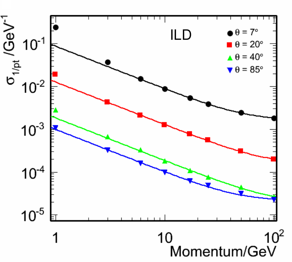
Figure 7: Inverse transverse momentum resolution estimated from fully simulated and reconstructed single muons at various momenta and polar angles for the ILD detector design and hit resolutions documented in [16]. The superimposed curves are fits over the [10, 100] GeV momentum range for the $a,b$ parameters of Eq. 11 at each of the displayed polar angles.

$\theta(^{\circ})$	$a$ ( $10^{-5}$ GeV-1)	$b$ ($10^{-3}$)
85	2.09	0.978
40	1.96	0.755
20	15.4	1.48
7	161	1.29

Table 5: Values for the $a,b$ parameters fitted to the high momentum range of Fig. 7 for four values of polar angle.

The combined effect of the momentum resolution of both muons on the $\sqrt{s}_{p}$ estimator is non-trivial as the momentum resolution depends significantly on the muon polar angle especially once tracks no longer benefit from the full radial track length in the TPC. The resolution is evaluated with a toy Monte Carlo simulation using the parametrization of the ILD tracking resolution described above. Figure 8 shows the intrinsic effect of tracking resolution on the reconstructed $\sqrt{s}_{p}$ estimate for two idealized cases as a function of center-of-mass energy, namely,

1. The $2\to 2$ “full energy” process ($\mathrm{e}^{+}\mathrm{e}^{-}\to\mu^{+}\mu^{-}$) with no additional photons for various scattering angles from $20^{\circ}$ to $90^{\circ}$.

2. The $\mathrm{e}^{+}\mathrm{e}^{-}\to\mathrm{Z}\gamma\to\mu^{+}\mu^{-}\gamma$ “radiative return” process where the photon is a collinear ISR photon and the dimuon mass is $m_{\mathrm{Z}}$. The scattering angle in the Z rest frame is set to $90^{\circ}$.

Also included in the figure as a separate component is the intrinsic beam energy spread contribution described earlier. The fractional resolution on $\sqrt{s}_{p}$ for full energy events depends markedly on the scattering angle being typically less than 0.2% for $\sqrt{s}\leq 250$ GeV in the barrel. The radiative return events (light blue curve) have a fractional resolution of as good as 0.1% when both muon tracks are well measured in the barrel. This degrades quickly at higher center-of-mass energies as the Z is more boosted and the resulting muons from the Z decay are more forward.

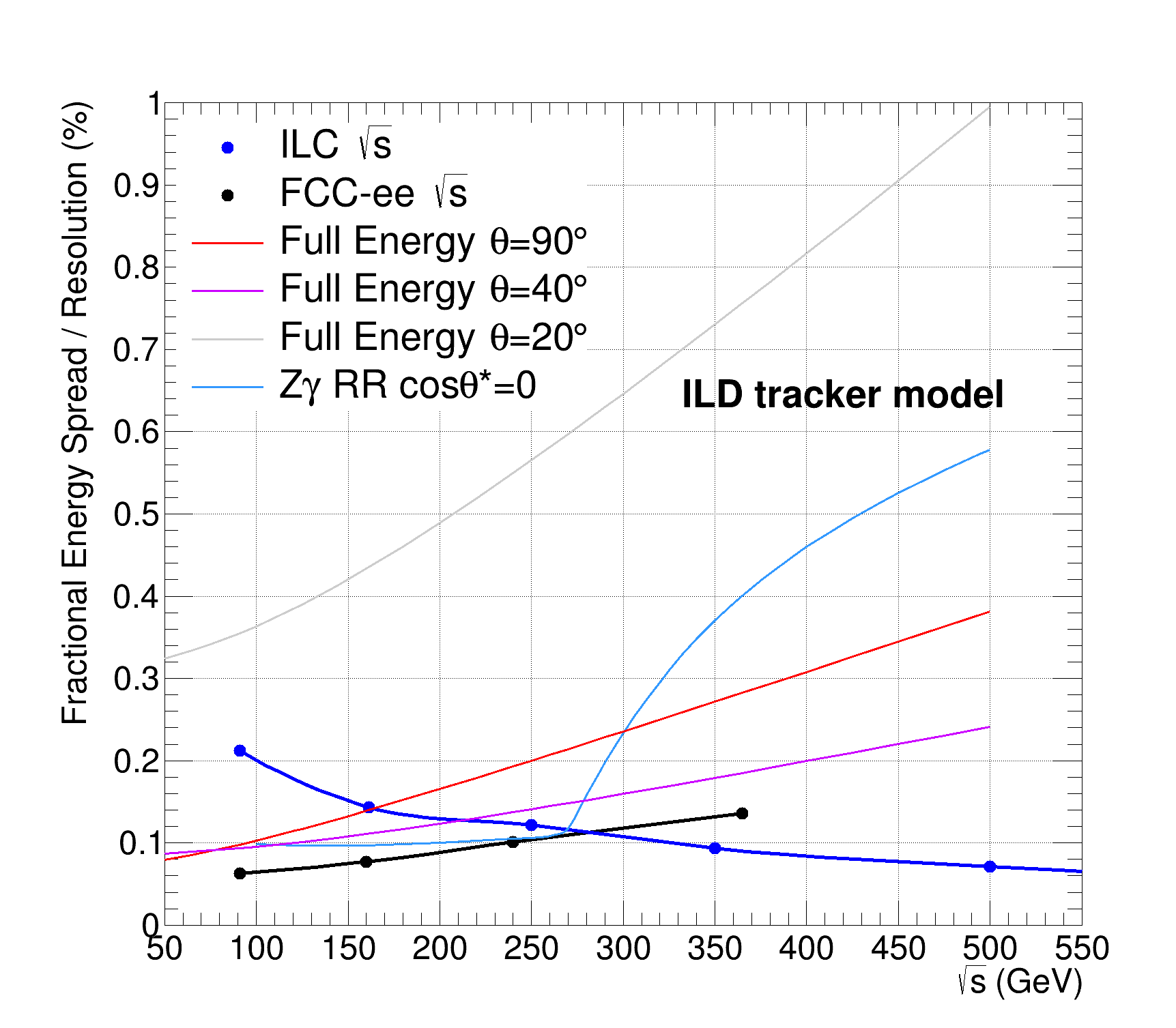
Figure 8: Center-of-mass energy dependence of the fractional resolution on $\sqrt{s}_{p}$ for the various configurations described in the text using the ILD tracker model.

7 Kinematic Acceptance

Given the strong dependence of the $\sqrt{s}_{p}$ resolution on polar angle, it is important to assess the fraction of dimuon events that will pass various acceptance cuts. The kinematics of the $\mathrm{e}^{+}\mathrm{e}^{-}\rightarrow\mu^{+}\mu^{-}(\gamma)$ process are characterized by the invariant mass of the dimuon system and the presence or not of detectable photons. The $\sqrt{s}_{p}$ method is permissive of the presence of one photon, but is susceptible to errors from events with multiple photons with a corresponding substantial mass to the photonic system. One way to elucidate the presence of photons where the photonic system has substantial transverse momentum, is to examine the acoplanarity angle,

$$\phi_{\text{acop}}\equiv\pi-\cos^{-1}\left(\mathrm{\hat{\mathbf{p}}}^{\text{T}}_{1}\cdot\mathrm{\hat{\mathbf{p}}}^{\text{T}}_{2}\right)\>\>,$$

where $\mathrm{\hat{\mathbf{p}}}^{\text{T}}_{1},\mathrm{\hat{\mathbf{p}}}^{\text{T}}_{2}$ are unit vectors in the directions of the transverse momenta of each muon. For these detector and physics reasons, it is expected that events with the muons in the barrel acceptance will be better measured and that coplanar events with small acoplanarity angles will be less sensitive to radiative corrections. Of course hard cuts on such quantities will also reduce the achievable statistical precision so one approach as followed in [1] is to categorize selected events by resolution quality thus avoiding unnecessary event loss. Figure 9 shows an evaluation of the acceptance dependence on center-of-mass energy for various choices of the acceptance requirements. One sees that the acceptance varies strongly with center-of-mass energy reflecting the substantial fraction of events from strong radiative return to much lower reduced center-of-mass energies including the Z and below where one or more muons are rather forward and often undetectable. However, even at $\sqrt{s}=1$ TeV, the drop in acceptance for the best measured events compared with $\sqrt{s}=250$ GeV is not that large despite the lack of accepted radiative return to the Z events.

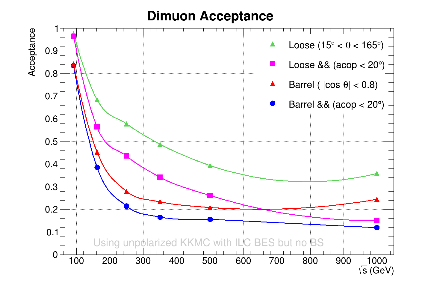
Figure 9: Kinematic acceptance dependence on center-of-mass energy for $\mathrm{e}^{+}\mathrm{e}^{-}\rightarrow\mu^{+}\mu^{-}(\gamma)$ evaluated using KKMC. Here the event generation is unpolarized and includes beam energy spread but not beamstrahlung. Shown are acceptance values for different polar angle requirements on the muons (loose and barrel). Also shown is an additional requirement of $\phi_{\text{acop}}<20^{\circ}$ (shown in purple for loose and blue for barrel).

8 Physics Limitations

The physical precision method described in [17] is used to evaluate quantitatively how much different levels of higher-order QED effects are needed to describe accurately the center-of-mass energy related observables. Weighted events from the KKMCee (4.32) generator [18] were used to re-weight the estimators at generator level ($\sqrt{s}_{p}$, $E^{\text{C}}_{-}$ and $E^{\text{C}}_{+}$) to alternative physics levels. The KKMCee event generator uses exclusive exponentiation (EEX) and coherent exclusive exponentiation (CEEX). The standard best estimate is ${\cal O}(\alpha^{2})$ CEEX denoted CEEX2. It is also possible to reweight to other models with a different, often less complete physics description, as follows:

• ${\cal O}(\alpha)$ CEEX (denoted CEEX1)

• ${\cal O}(\alpha^{3})$ EEX (denoted EEX3)

• ${\cal O}(\alpha^{2})$ CEEX but no ISR/FSR interference (denoted CNIF2)

Table 6 shows the $\sqrt{s}_{p}$ physical precision estimates for $\sqrt{s}_{p}$ in parts per million (ppm) for the CEEX1, EEX3, and CNIF2 variations compared to CEEX2. For this comparison, the barrel acceptance with a 20^∘ acoplanarity requirement (the blue curve of Fig. 9) was used. The simulations used 10 million unpolarized weighted events per $\sqrt{s}$ and included ILC beam energy spread but no beamstrahlung.

$\sqrt{s}$ (GeV)	CEEX1	EEX3	CNIF2
91	-0.9	0.4	0.02
161	-0.2	-10	-11
250	-0.3	-11	-11
350	-0.6	-10	-10
500	-0.5	-9	-9
1000	-0.6	-8	-8

Table 6: Calculated physical precision in ppm in the $\sqrt{s}_{p}$ observable vs center-of-mass energy for the CEEX1, EEX3, and CNIF2 variations compared to the CEEX2 setting. The mean value for each setting of $(\sqrt{s}_{p}-\sqrt{s})/\sqrt{s_{\mathrm{nom}}}$ is calculated using a $\pm 0.5$% range. The quoted number is half the observed difference following the convention in [17].

The recommended comparison is CEEX2 with CEEX1; for this case the physical precision for all center-of-mass energies studied is below the ppm level. Studies without the acoplanarity cut indicate that the acoplanarity cut is needed to achieve this level of physical precision for the CEEX2 with CEEX1 comparison especially at high $\sqrt{s}$. For the comparisons with EEX3 and CNIF2 the observed order of magnitude worse physical precision of approximately 10 ppm of Table 6 is also found without the acoplanarity cut. Similar qualitative results to Table 6 were observed for the $E^{\mathrm{C}}_{-}$ and $E^{\mathrm{C}}_{+}$ observables but with typically a factor of 3–4 larger physical precision values calculated for a $\pm 2$% range. In conclusion, it appears that the QED effects on the observables studied are already under astonishingly good control and for the $\sqrt{s}_{p}$ observable at a level of one part per million (with the acoplanarity angle requirement to suppress higher order effects). Therefore, based on these considerations of calculational accuracy, there are excellent prospects for including higher-order QED effects with sufficient precision in the $\mathrm{e}^{+}\mathrm{e}^{-}\rightarrow\mu^{+}\mu^{-}(\gamma)$ channel.

9 Bhabhas

Figure 10 illustrates the statistical advantage that is available from Bhabha events compared to dimuon events versus center-of-mass energy. The $\sqrt{s}_{p}$ method for center-of-mass energy relies on precision tracking momentum resolution. As an example, the barrel Bhabha cross-section at $\sqrt{s}=250$ GeV of 24 pb exceeds the accepted dimuon barrel cross-section of 1.5 pb by a factor of sixteen. The wide-angle Bhabha cross-sections were evaluated with version 1.05 of BHWIDE [19].

Therefore, depending on how well electron tracks can be reconstructed compared with muon tracks, and their momentum-scale controlled, the expected overall sensitivity using $\sqrt{s}_{p}$ can be much better than that from the dimuon channel alone such as reported in [1]. This is especially true at center-of-mass energies above the Z where the $t$-channel enhancement of Bhabha scattering at wide angle is most prominent. In the context of typical detector designs, the still much larger cross-section at forward angles needs to be tempered by the worsening tracking resolution at forward angles beyond the barrel region (see for example Fig. 8 for the ILD tracker model). Nevertheless, the statistical precision afforded by Bhabha events will certainly be key to improving the monitoring of the time variation of the center-of-mass energy scale.

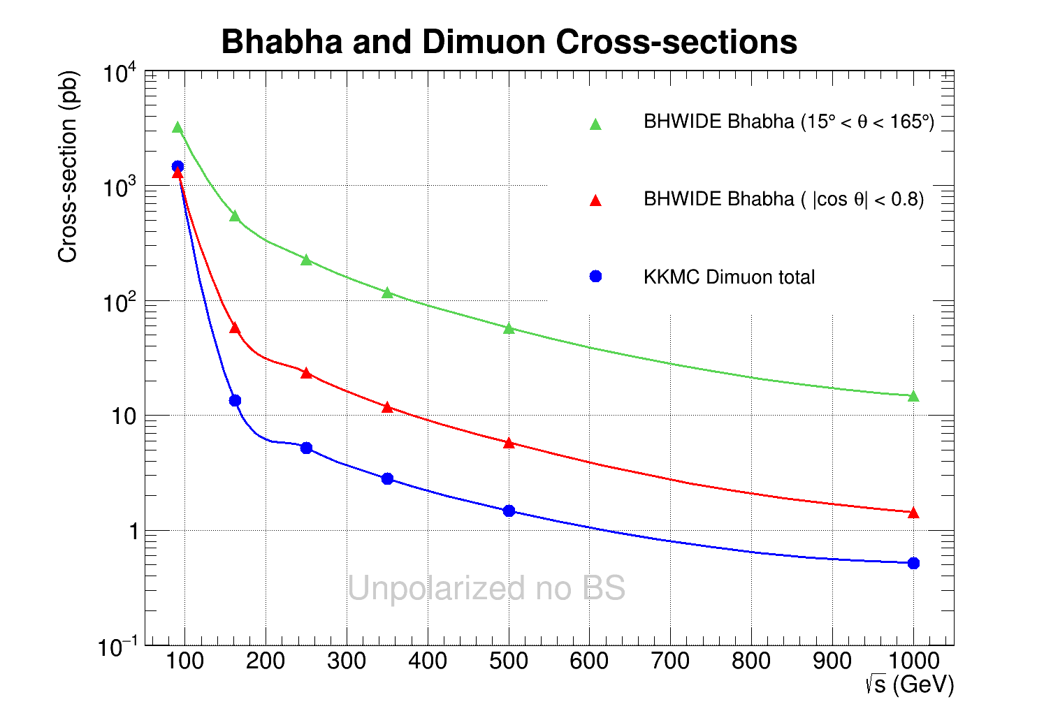
Figure 10: Calculated cross-sections in pb vs center-of-mass energy for the Bhabha process $\mathrm{e}^{+}\mathrm{e}^{-}\to\mathrm{e}^{+}\mathrm{e}^{-}(\gamma)$ for both a barrel acceptance for the detected $\mathrm{e}^{+}$ and $\mathrm{e}^{-}$ in red ($|\cos{\theta}|<0.8$) and a wider acceptance in green ($15^{\circ}<\theta<165^{\circ}$) using BHWIDE and for $\mathrm{e}^{+}\mathrm{e}^{-}\rightarrow\mu^{+}\mu^{-}(\gamma)$ in blue using KKMC (no acceptance cuts). The cross-section calculations are unpolarized and neglect beamstrahlung and beam energy spread effects.

10 Summary and Outlook

Developments related to the measurement of the center-of-mass energy using dilepton events at future $\mathrm{e}^{+}\mathrm{e}^{-}$ colliders have been described. Two new estimators were introduced related to the energy of the colliding electron and positron thus permitting more direct study of the 2-d luminosity spectrum marginal distributions. Further work is need to fully exploit these. We developed a parametric model for the 2-d luminosity spectrum that includes modeling of the dependence structure using copulas and a simplified treatment of beam energy spread. This model should be straightforward to implement in event generators.

We also surveyed issues associated with the $\sqrt{s}_{p}$ momentum-based center-of-mass energy estimator for center-of-mass energies in the 90 GeV to 1 TeV range including beam energy spread, detector momentum resolution, kinematic acceptance, theoretical uncertainties, and the use of the Bhabha channel. Overall we are very encouraged that these techniques can target 1 ppm precision on the center-of-mass energy scale thus facilitating precision mass measurements. A primary need is control of the detector momentum scale at the targeted precision; strategies for this have been outlined but will need to be thoroughly assessed. A full quantitative assessment of the prospects with the $\sqrt{s}_{p}$ and related methods for all $\sqrt{s}$ requires an overall consistent estimation procedure including modeling of beamstrahlung, beam energy spread, polarization, detector effects, state-of-the-art radiative effects, the inclusion of Bhabhas, and an estimator calibration procedure; this was beyond the scope of the current work.

Appendix A Fit models

We have used a new fit model to characterize the expected sensitivity to the center-of-mass energy scale parameter and to model the shape of related distributions. This new model is based on convolving a CIRCE-like function with a Gaussian response function to model beam energy spread or detector resolution. In our earlier work [1] we had used two fit models: the well known Crystal Ball function, and the convolution of a Gaussian response function with a mixture of a two-component exponential for the low energy tail and a delta function for the peak. The latter more flexible fit model was chosen partly for convenience since it is analytically integrable. Details of the latest model and its implementation using numerical integration are described below. For completeness we also describe the fit model used for the pre beam energy spread distributions.

A.1 Gaussian peak and convolved beta tail

Previous work on fitting the electron and positron energy distributions absent beam energy spread effects had been done using a mixture of a beta distribution for the beamstrahlung tail and a delta function for the undisturbed peak in CIRCE [8]. Here we apply similar methodology to either the center-of-mass energy or single beam energy distributions but taking into account a Gaussian response function using convolution. We define the scaled true energy, $x=E/E_{0}$, where $E$ is the true energy, and $E_{0}$ is the energy scale parameter. The resulting probability density function of the fit model at convolved scaled energy, $x^{\prime}=E^{\prime}/E_{0}$, has 5 parameters, and is given by

$$p(x^{\prime};\alpha,\beta,\sigma,E_{0},f_{\mathrm{peak}})=\int_{0}^{1}[f_{\mathrm{peak}}\delta(x-1)+\frac{(1-f_{\mathrm{peak}})}{B(\alpha,\beta)}x^{\alpha-1}(1-x)^{\beta-1}]\;G(x^{\prime}-x;\;\sigma)dx\;\text{,}$$ (12)

where $E^{\prime}$ is the convolved energy, $\alpha$ and $\beta$ are the beta distribution parameters, $f_{\mathrm{peak}}$ is the fraction associated with the delta function component located at $x=1$, $\sigma$ is the standard deviation of the Gaussian response function as a fraction, and the normalizing coefficient is

$$B(\alpha,\beta)=\frac{\Gamma(\alpha)\Gamma(\beta)}{\Gamma(\alpha+\beta)}\>,$$ (13)

where $\Gamma$ is the Gamma function. The Gaussian response function is simply,

$$G(x^{\prime}-x;\;\sigma)=\frac{1}{\sqrt{2\pi\sigma^{2}}}\exp\left(-\frac{(x^{\prime}-x)^{2}}{2\sigma^{2}}\right)\;\text{,}$$ (14)

which smears deviations from the true scaled energy, $x$, of size, $x^{\prime}-x$, with resolution, $\sigma$.

As in CIRCE, a variable transformation is used to take care of the integrable singularity of the beta distribution at $x=1$. Multiple numerical integration methods for the convolution were tested particularly with a view to the stability and speed of the fit procedure. For this work 30-point Gauss-Legendre integration over a $\pm 6\sigma$ integration window was used for the probability density evaluation and the fit was implemented using RooFit [20].

This 5-parameter fit function manages to describe the simulated Guinea-PIG data, which includes beam energy spread effects, much better or with fewer parameters than the two prior models. Therefore we have adopted it as the preferred empirical fit model for center-of-mass energy and beam energy distributions.

A.2 Double beta tail

For the fits to the Body and Arms regions of the pre beam energy spread marginal distributions we fit a 5-parameter two-component model with two beta functions to each $x$ distribution as follows

$$p(x;\alpha_{1},\beta_{1},\alpha_{2},\beta_{2},f_{1})=\frac{f_{1}}{B(\alpha_{1},\beta_{1})}x^{\alpha_{1}-1}(1-x)^{\beta_{1}-1}+\frac{(1-f_{1})}{B(\alpha_{2},\beta_{2})}x^{\alpha_{2}-1}(1-x)^{\beta_{2}-1}\>\>\text{.}$$ (15)

References

- [1] B. Madison and G.W. Wilson “Center-of-mass energy determination using events at future colliders,” arXiv:2209.03281.
- [2] W. Kilian, T. Ohl, and J. Reuter, “WHIZARD: Simulating Multi-Particle Processes at LHC and ILC,” Eur. Phys. J. C 71, 1742 (2011), arXiv:0708.4233.
- [3] M. Moretti, T. Ohl, and J. Reuter, “O’Mega: An Optimizing matrix element generator,” arXiv:0102195.
- [4] A. Aryshev et al. [ILC International Development Team], “The International Linear Collider: Report to Snowmass 2021,” arXiv:2203.07622.
- [5] K. Yokoya, K. Kubo, and T. Okugi, “Operation of ILC250 at the Z-pole,” arXiv:1908.08212.
- [6] D. Schulte, “Study of Electromagnetic and Hadronic Background in the Interaction Region of the TESLA Collider,”, Ph.D. Thesis, University of Hamburg (1996), DESY-TESLA-97-08.
- [7] S. Poss and A. Sailer, “Luminosity Spectrum Reconstruction at Linear Colliders,” Eur. Phys. J. C 74 (2014) 2833, arXiv:1309.0372.
- [8] T. Ohl, “CIRCE version 1.02: Beam spectra for simulating linear collider physics,” Comput. Phys. Commun. 101 (1997) 269, arXiv:9607454.
- [9] B. Madison, “Using the GP2X framework for center-of-mass energy precision studies at Higgs factories,” these proceedings, arXiv:2308.09676.
- [10] A. P. Sailer, “Studies of the measurement of differential luminosity using Bhabha events at the International Linear Collider,” Masters Thesis, Humboldt University, Berlin (2009), DESY-THESIS-2009-011.
- [11] C. Rimbault et al., “GUINEA PIG++: An Upgraded Version of the Linear Collider Beam Beam Interaction Simulation Code GUINEA PIG,” Conf. Proc. C 070625 (2007), 2728 PAC.2007.4440556
- [12] R. B. Nelsen, “An Introduction to Copulas”, 2nd Edition, Springer, 2006.
- [13] H. Joe, “Dependence Modeling with Copulas”, CRC Press, 2015.
- [14] G. G. Venter, “Tails of copulas”, Proc. of the Casualty Actuarial Society LXXXIX No. 171 (2002) 68.
- [15] C. Genest, B. Rémillard, and D. Beaudoin, “Goodness-of-fit tests for copulas: A review and a power study”, Insurance: Mathematics and Economics 44 (2009) 199.
- [16] T. Behnke et al. “The International Linear Collider Technical Design Report - Volume 4: Detectors,” arXiv:1306.6329.
- [17] S. Jadach, B. F. L. Ward, and Z. Was, “The Precision Monte Carlo event generator KK for two-fermion final states in collisions,” Comput. Phys. Commun. 130 (2000), 260, arXiv:9912214.
- [18] S. Jadach, B. F. L. Ward, Z. Was, S. A. Yost, and A. Siodmok, “Multi-photon Monte Carlo event generator KKMCee for lepton and quark pair production in lepton colliders,” Comput. Phys. Commun. 283 (2023), 108556, arXiv:2204.11949.
- [19] S. Jadach, W. Placzek, and B. F. L. Ward, “BHWIDE 1.00: () YFS exponentiated Monte Carlo for Bhabha scattering at wide angles for LEP-1 / SLC and LEP-2,” Phys. Lett. B 390 (1997), 298, arXiv:9608412.
- [20] W. Verkerke and D. P. Kirkby, “The RooFit toolkit for data modeling,” eConf C0303241, MOLT007 (2003), arXiv:0306116.