HoSNN: Adversarially-Robust Homeostatic Spiking Neural Networks with Adaptive Firing Thresholds

Abstract

Spiking neural networks (SNNs) offer promise for efficient and powerful neurally inspired computation. Common to other types of neural networks, however, SNNs face the severe issue of vulnerability to adversarial attacks. We present the first study that draws inspiration from neural homeostasis to develop a bio-inspired solution that counters the susceptibilities of SNNs to adversarial onslaughts. At the heart of our approach is a novel threshold-adapting leaky integrate-and-fire (TA-LIF) neuron model, which we adopt to construct the proposed adversarially robust homeostatic SNN (HoSNN). Distinct from traditional LIF models, our TA-LIF model incorporates a self-stabilizing dynamic thresholding mechanism, curtailing adversarial noise propagation and safeguarding the robustness of HoSNNs in an unsupervised manner. Theoretical analysis is presented to shed light on the stability and convergence properties of the TA-LIF neurons, underscoring their superior dynamic robustness under input distributional shifts over traditional LIF neurons. Remarkably, without explicit adversarial training, our HoSNNs demonstrate inherent robustness on CIFAR-10, with accuracy improvements to 72.6% and 54.19% against FGSM and PGD attacks, up from 20.97% and 0.6%, respectively. Furthermore, with minimal FGSM adversarial training, our HoSNNs surpass previous models by 29.99% under FGSM and 47.83% under PGD attacks on CIFAR-10. Our findings offer a new perspective on harnessing biological principles for bolstering SNNs adversarial robustness and defense, paving the way to more resilient neuromorphic computing.

Introduction

Neural networks have demonstrated remarkable capabilities across various tasks, yet they are notoriously susceptible to adversarial attacks. These attacks perturb the input data subtly, leading well-trained models to misclassify while the perturbations remain virtually invisible to human observers. This vulnerability, initially discovered in the early works of (Szegedy et al. 2013), threatens the reliability of neural networks as they are increasingly deployed in safety-critical applications such as autonomous vehicles and medical imaging. Addressing this issue not only ensures trustworthiness in AI systems but also has remained a vital research focus in contemporary machine learning.

Over the years, significant strides have been made in the field of adversarial robustness to generate adversarial examples, including the Fast Gradient Sign Method (FGSM) (Goodfellow, Shlens, and Szegedy 2014), DeepFool (Moosavi-Dezfooli, Fawzi, and Frossard 2016), and Projected Gradient Descent (Madry et al. 2017). Among various defense strategies, adversarial training has proven effective. Yet, it is not without limitations, as it grapples with high computational costs and challenges in migrating between different attack paradigms. This complexity underlines the need for novel perspectives and methods to improve robustness in neural networks.

SNNs simulate the way biological neurons convey information via spikes. Originating in the early 1990s, SNNs research introduced models such as the Spike Response Model (SRM) and the Leaky Integrate-and-Fire (LIF) model (Gerstner and Kistler 2002). The focus in SNNs has been on learning algorithms, architectures, and spike coding. With industry players like IBM and Intel delving into SNNs hardware, innovations such as IBM’s TrueNorth (Merolla et al. 2014) and Intel’s Loihi (Davies et al. 2018) have emerged. These devices exploit SNNs’ efficiency, highlighting their potential for neuromorphic computing and advancing our grasp of biological neural mechanisms (Furber et al. 2014).

However, the question of robustness in SNNs remains underexplored. Despite sharing vulnerabilities to adversarial attacks with their non-spiking counterparts (Sharmin et al. 2019, 2020), SNNs pose an intriguing contradiction. In nature, biological neural systems, which SNNs aim to emulate, demonstrate resilience against a variety of perturbations and noise, rarely exhibiting the susceptibilities seen in artificial networks (Turrigiano and Nelson 2004). This disparity in SNNs prompts a reassessment of their design and principles, suggesting that enhancing robustness not only defends against adversarial attacks but also narrows the gap between artificial and biological neural systems, deepening our understanding of both domains (Lillicrap et al. 2020). Meanwhile, current research on SNNs robustness often neglects the biological interpretability of SNNs and the dynamics of LIF neurons, facing issues such as high computational costs and low transferability.

In light of such dilemmas, we ask: Why are biological nervous systems impervious to adversarial noise? How do homeostatic mechanisms contribute to the robustness of network activity? Can we exploit the dynamics of SNNs to suppress the propagation of adversarial noise by homeostatic mechanisms? Our investigation, inspired by the inherent robustness of biological neural systems against adversarial perturbations, aims to address these questions. The key contributions of our work can be summarized as :

• We first connect the biological homeostasis mechanism and adversarial robustness in SNNs, introducing an efficient and effective bio-inspired solution to address the vulnerabilities of SNNs under adversarial attacks.

• We introduce the Neural Dynamic Signature (NDS), which encapsulates the activation degree of specific semantic information represented by each neuron and serves as an anchor signal to stabilize neuron behaviors against distributional shifts.

• We design a novel threshold-adapting leaky integrate-and-fire (TA-LIF) neuron model, which incorporates a self-stabilizing thresholding mechanism. Theoretical analysis confirms that our model can suppress the propagation of out-of-distributional noise in an unsupervised way.

• Building upon TA-LIF neurons, we introduce the inherently adversarially robust Homeostatic SNN (HoSNN) and demonstrate that its training algorithm can seamlessly integrate with various SNN learning methods, without significant computational overhead.

• Our experiments demonstrate that HoSNNs consistently exhibit inherent robustness in image classification tasks even without adversarial training, and further amplify the benefits of adversarial training when applied. Notably, our results either surpass or closely align with state-of-the-art benchmarks.

Related Work

Adversarial Attacks

Adversarial perturbations continue to pose a significant challenge in deep learning. By exploiting the intricacies of high-dimensional data and non-linear mappings in a model, these subtle but well-crafted alterations can cause drastic changes to model predictions. Such attacks extend beyond the realm of theoretical interest, posing genuine risks in practical applications ranging from autonomous vehicles to medical imaging (Akhtar and Mian 2018).

Two notable adversarial attack techniques are the Fast Gradient Sign Method (FGSM) (Goodfellow, Shlens, and Szegedy 2014) and the Projected Gradient Descent (PGD) (Madry et al. 2017). FGSM uses the loss gradients concerning input data to quickly produce adversarial samples. Let $x$ be the original input, $y$ the true label, $J(\theta,x,y)$ the loss function with network parameters $\theta$, and $\epsilon$ a small perturbation magnitude. The FGSM perturbed input $x^{\prime}$ is:

$$x^{\prime}=x+\epsilon\cdot sign(\nabla_{x}J(\theta,x,y))$$ (1)

PGD is essentially an iterative FGSM, modifies data over iterations. With $x_{n}$ as the perturbed input in the n-th iteration and $\alpha$ as the step size, PGD updates by:

$$x_{n+1}=Proj_{x+\epsilon}(x_{n}+\alpha\cdot sign(\nabla_{x}J(\theta,x_{n},y)))$$ (2)

More gradient-based attacks work in a similar fashion, such as the RFGSM (Tramèr et al. 2017), a randomized version of FGSM and the Basic Iterative Method (BIM) (Kurakin, Goodfellow, and Bengio 2018) as another iterative attack.

Adversarial attacks extend beyond the core concepts of gradient-based methods. A wide array of techniques with varied objectives exists, underlining the pressing need for advances in adversarial robustness research (Biggio and Roli 2018). A significant area of concern is the rise of black-box attacks. These occur when an attacker, with limited model knowledge, successfully crafts adversarial examples using transferability. This phenomenon, where adversarial samples created for one model compromise another, underscores the profound vulnerabilities of neural networks and presents significant security concerns (Papernot, McDaniel, and Goodfellow 2016).

Defense Methods

To combat adversarial threats, researchers have explored a plethora of defense strategies. Adversarial training focuses on retraining the model using a mixture of clean and adversarial examples (Madry et al. 2017). Moreover, the Randomization technique introduces stochasticity during the inference phase to prevent precise adversarial attacks (Xie et al. 2017). The Projection technique can revert these inputs back to a safer set, neutralizing the effects of the perturbations (Mustafa et al. 2019). Lastly, the Detection strategy serves as a safeguard by identifying and responding to altered inputs (Metzen et al. 2017).

While these defense methods offer an added layer of protection against adversarial attacks, each has its limitations (Akhtar and Mian 2018). Adversarial Training, despite its effectiveness, is computationally expensive, can result in loss of accuracy on clean inputs, and is often difficult to transfer between different models. Randomization, projection, and detection strategies, on the other hand, don’t fundamentally address the inherent vulnerabilities of neural networks. Thus, despite these methods providing incremental improvements to the robustness of a model, no single technique offers universal effectiveness.

Moreover, in the context of SNNs, which are valued for their biological plausibility, these methods are generally not considered biologically feasible. Thus, there’s an urgent need for more efficient and biologically plausible solutions to enhance the robustness of neural networks, particularly for SNNs.

Spiking Neural Networks Robustness

With the rise in popularity of SNNs for real-world applications, from odor recognition (Imam and Cleland 2020) to autonomous driving (Pei et al. 2019) the robustness of these networks has become a significant concern. Empirical studies have demonstrated that SNNs, analogous to artificial neural networks (ANNs), exhibit similar susceptibilities to adversarial attacks (Sharmin et al. 2019; Ding et al. 2022).

A line of inquiry in this field has explored porting defensive strategies from ANNs to SNNs. For instance, (Kundu, Pedram, and Beerel 2021) proposed an SNNs training algorithm that enhances resilience by jointly optimizing thresholds and weights. (Ding et al. 2022) proposed a method of adversarial training enhanced by a Lipschitz constant regularizer. (Liang et al. 2022) established the boundaries for LIF neurons and designed corresponding certified training methods in SNNs. However, these works lack biological plausibility, a defining characteristic of SNNs. Additionally, they seem to import the shortcomings of ANNs defensive methods into SNNs, including expensive computational cost and transferability of defense methods between different attacks

Another research direction has focused on studying the inherent robustness of SNNs, examining factors such as agent gradient algorithms, encoding methods, and hyperparameters. For example, (Sharmin et al. 2020) recognized the inherent resistance of SNNs to gradient-based adversarial attacks. (El-Allami et al. 2021) investigated the impact of internal structural parameters, such as firing voltage thresholds and time window boundaries. (Chowdhury, Lee, and Roy 2021) underscored the robustness of the LIF model, particularly its noise-filtering capability. (Li et al. 2022) explored the influence of network inter-layer sparsity and (Xu et al. 2022) examined the effects of surrogate gradient techniques on white-box attacks. Despite these advances, most studies fail to present effective SNNs defense strategies. More importantly, two key facts were ignored: first, the biological neural systems that SNNs aim to simulate rarely exhibit adversarial vulnerability; while little attention has been paid to the link between homeostatic mechanisms and network robustness. Second, the dynamical characteristics of LIF neurons, a crucial difference between SNNs and ANNs, have not been thoroughly examined, particularly their stability under disturbances.

These observations motivate our work, aiming to simulate the homeostasis of the biological nervous system at the level of single neurons to develop a naturally robust SNN.

Methods

We initiate our exploration by examining the dynamic activations of individual neurons, which we coin as the “Neural Dynamic Signature” (NDS). Drawing insights from the principle of biological homeostasis, we introduce and rigorously analyze a threshold-adapting leaky integrate-and-fire model (TA-LIF) with an objective of stabilizing neuronal dynamics. Subsequently, we delineate a variant of SNNs that incorporates TA-LIF neurons, referred to as homeostatic SNNs (HoSNNs).

Neural Dynamic Signature (NDS)

Let $\mathcal{D}$ represent the in-domain input data distribution with samples $x$ possessing corresponding labels $l$ used to train a SNN model with parameters $\theta_{\mathcal{D}}$, which yields a prediction $y(x|\theta_{\mathcal{D}})$ for $x$. Upon introduction of adversarial noise, denoted by $\delta x$, a perturbed sample $x+\delta x$ emerges from an altered distribution $\mathcal{D^{\prime}}$, resulting in a divergent prediction $y^{\prime}(x+\delta x|\theta_{\mathcal{D}})$. Such crafted perturbations typically misguide the network, predominantly influencing neurons encapsulating pivotal semantic information (Li et al. 2021). This perturbation magnifies neuronal activity discrepancies through cascading layer interactions, culminating in a stark divergence between $y$ and $y^{\prime}$. The subtle shift from $\mathcal{D}$ to $\mathcal{D^{\prime}}$ jeopardizes model accuracy, rendering the finely-tuned parameter $\theta_{\mathcal{D}}$ suboptimal or even completely ineffective (Rabanser, Günnemann, and Lipton 2019; Nadhamuni 2021; Shu et al. 2020; Fawzi, Moosavi-Dezfooli, and Frossard 2016; Ford et al. 2019; Kang et al. 2019; Ilyas et al. 2019).

In conventional ANNs, a neuron’s output typically signifies the activation degree of its semantic representation, although such distributed encoding often eludes straightforward human interpretation (Bills et al. 2023). Unlike ANNs, SNNs operate in a spatiotemporal manner over a richer set of variables including the time-indexed membrane potential $u_{i}(t)$ for each neuron $i$, which is a key state variable and dictates neuron $i$’s output spike trains. Under the context of learning, we take a step forward by using the membrane potential $u_{i}(t)$ series as a nuanced representation of the semantic vector, with the meaning of the activation intensity of the semantic information it represents.

Although the membrane potential $u_{i}(t)$ of neuron $i$ might exhibit variability across individual samples $x$, its expected value over distribution $\mathcal{D}$, denoted by $\mathbb{E}_{x\sim\mathcal{D}}[u_{i}(t|x)]$, serves as a reliable metric, encapsulating the averaged semantic activation over $\mathcal{D}$. As adversarial perturbations induce input distributional shifts, leading to anomalous activation or suppression of out-of-distributional semantics, this expected value offers an anchor signal, facilitating the identification of neuronal activation aberrations and bolstering network resilience.

For a given data instance $x$ sampled from distribution $\mathcal{D}$ , the Neural Dynamic Signature (NDS) of neuron $i$ contingent upon network parameters $\theta$ and the training set distribution $\mathcal{D}$ is articulated as a temporal series vector $\bm{\alpha_{i}}(\theta,\mathcal{D})$, which at time $t$ has value :

$$\bm{\alpha_{i}}(t_{k}|\theta,\mathcal{D})=\mathbb{E}_{x\sim\mathcal{D}}[u_{i}(t|\theta,x)],\text{for }t\in[0,T]$$ (3)

Drawing parallels with the Electroencephalogram (EEG) in biological systems, we conceive the network-level NDS, $\mathcal{A}_{\text{NET}}(\theta,\mathcal{D})$, as a set of individual neuron NDS vectors across the entirety of the SNN. Formally, the network-level NDS with a set of $N$ neurons is expressed as:

$$\mathcal{A}_{\text{NET}}(\theta,\mathcal{D})=\{\bm{\alpha}_{i}(\theta,\mathcal{D})\}_{i=1}^{N}$$ (4)

Densely populated SNNs have $O(N^{2})$ weight parameters. In contrast, $\mathcal{A}_{\text{NET}}(\theta,\mathcal{D})$ exhibits a scaling of $O(NT)$. Recent strides in SNNs algorithms, curbing $T$, the number of time steps over which the SNNs operate, to values such as 5 or 10 (Zhang and Li 2020). Thus, the computational and storage overhead of the NDS remains well tractable.

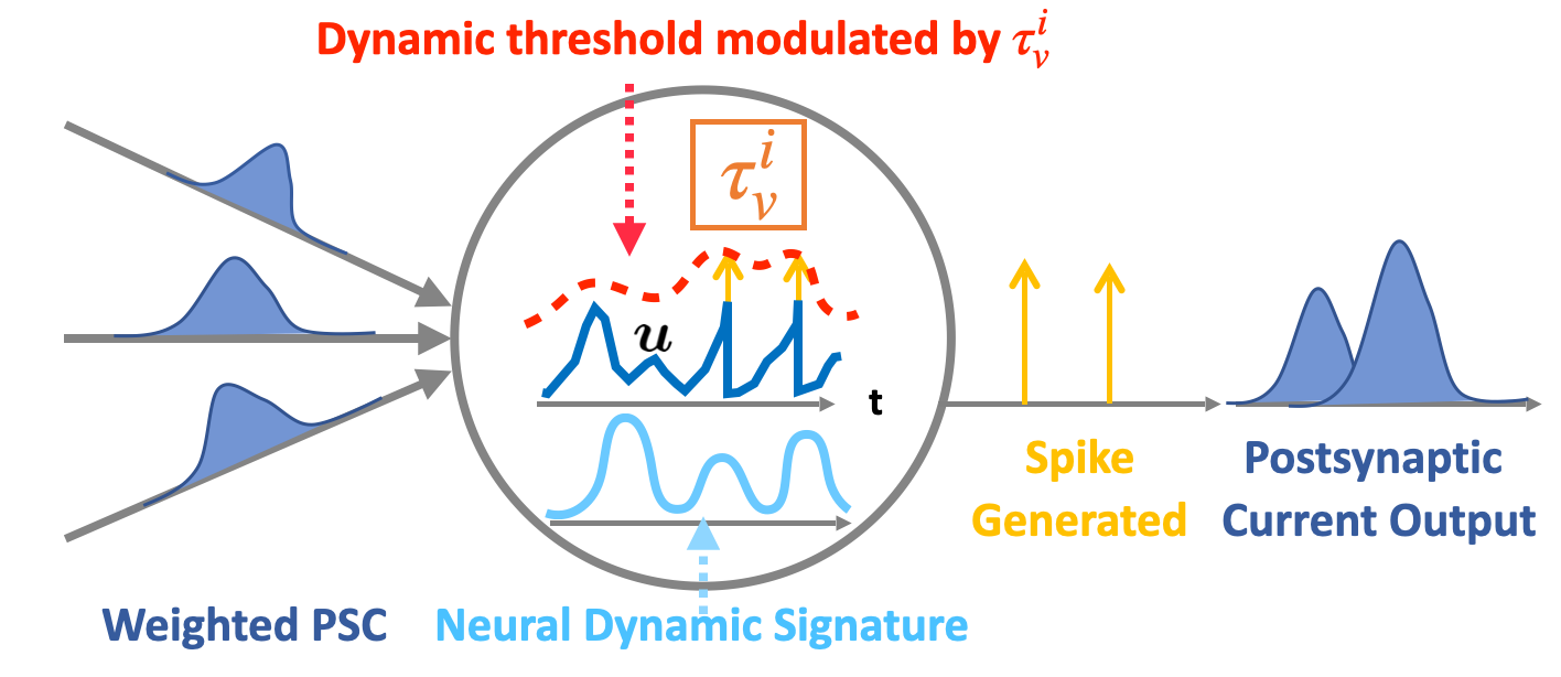
(a) Illustration of TA-LIF neurons.

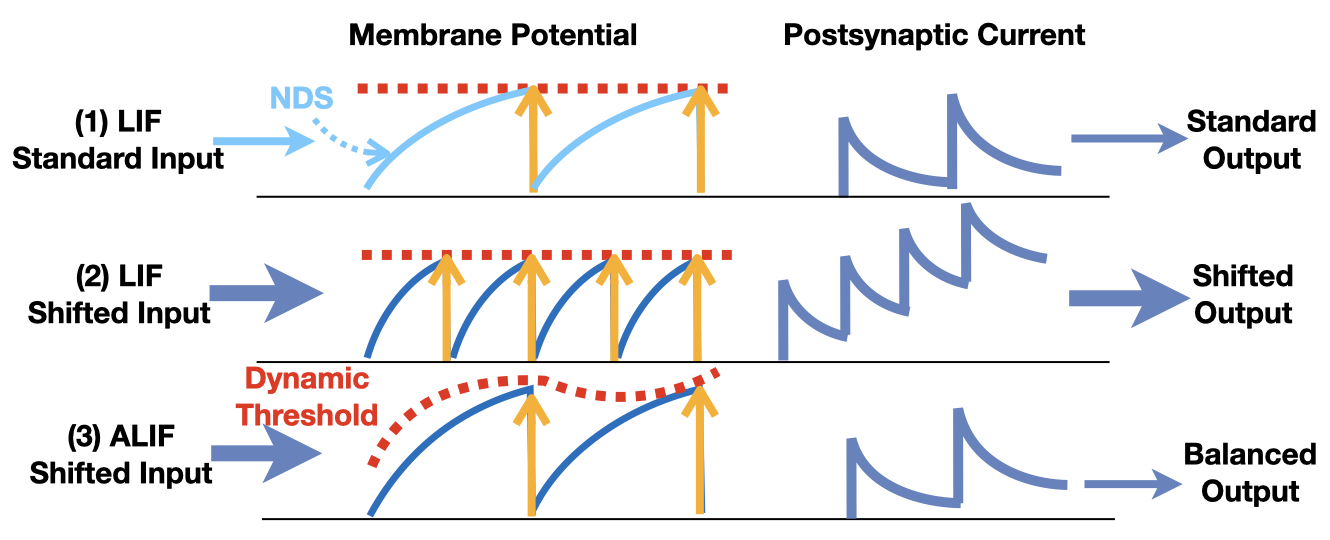
(b) Illustration of dynamic thresholds.

Figure 1: Illustration of TA-LIF neurons

Threshold-Adapting Leaky Integrate-and-Fire Spiking Neural Model (TA-LIF)

We proposed a Threshold-Adapting Leaky Integrate-and-Fire Spiking Neural Model (TA-LIF) incorporating a novel homeostatic self-stabilizing mechanism based on the neuron level NDS, ensuring that out-of-distributional input semantics do not excessively trigger abnormal neuron activity. We describe how our generally applicable self-stabilizing mechanism can be integrated with the LIF model with first order synapses.The dynamics of the LIF neuron $i$ at time $t$ is described by the membrane potential $u_{i}(t)$ and governed by the following differential equation:

$$\tau_{m}\frac{du_{i}(t)}{dt}=-u_{i}(t)+I(t)-\tau_{m}s_{i}(t)V_{th}^{i}(t)$$ (5)

where: $\tau_{m}$ is the membrane time constant; $I(t)$ represents the input and is defined as the sum of the pre-synaptic currents: $I(t)=R~{}\sum_{j}w_{ij}a_{j}(t)$; $w_{ij}$ represents the synaptic weight from neuron $j$ to neuron $i$; $a_{j}(t)$ is the post-synaptic current induced by neuron $j$ at time $t$; $V_{th}^{i}(t)$ is the firing threshold of neuron $i$ at time $t$. Neuron $i$’s postsynaptic spike train is:

$$s_{i}(t)=\begin{cases}+\infty&\text{if }u_{i}(t)\geq V^{i}_{th}(t)\\ 0&\text{otherwise}\end{cases}$$ (6)

which can also be expressed as the sum of the Dirac functions in terms of the postsynaptic spike times $t_{i}^{f}$:

$$s_{i}(t)=\sum_{f}\delta(t-t_{i}^{f})$$ (7)

With $\tau_{s}$ denoting the synaptic time constant, the evolution of the generated postsynaptic current (PSC) $a_{j}(t)$ is described by:

$$\tau_{s}\frac{da_{j}(t)}{dt}=-a_{j}(t)+s_{j}(t)$$ (8)

Threshold-Adapting Mechanism

In the traditional Leaky Integrate-and-Fire (LIF) model, the threshold $V_{th}$ is retained as a constant. Nevertheless, certain generalized LIF (GLIF) models have incorporated dynamic adjustments to $V_{th}$ through homeostatic mechanisms, mirroring observations in biological systems (AllenInstitute 2018). Notably, homeostatic mechanisms are imperative for stabilizing circuit functionality and modulating both intrinsic excitability and synaptic strength (Marder and Goaillard 2006). Several prevalent GLIF models are characterized by a tunable firing threshold with short-term memory, which increases with every emitted output spike and subsequently decays exponentially back to the foundational threshold (Bellec et al. 2018, 2020). However, such mechanisms often do not equip neurons with the requisite information to discern between “normal” and aberrant neural activity. There is no prior study leveraging homeostasis explicitly for adversarial robustness.

The key distinctions of the proposed homeostasis are exploration of the neuron-level Neural Dynamic Signature (NDS) as the anchor signal for threshold regulation and incorporation of an error signal defined based upon the NDS into the dynamics of the firing threshold. Concretely, for neuron $i$ in a HoSNN parameterized by weights $\theta$, if the membrane voltage $u_{i}(t|\theta,x)$ arises due to a canonical input $x$ sampled from distribution $\mathcal{D}$, and $u_{i}(t|\theta,x^{\prime})$ arises from an adversarial input $x^{\prime}=x+\delta x$ from distribution $\mathcal{D^{\prime}}$, our objective is to ensure that the resulting output firing activities are homogenized by modulating the threshold. The intuition guiding this is straightforward: if a neuron undergoes abnormal activation, the threshold should be heightened to restrain spike output. Conversely, if a neuron experiences abnormal inhibition, the threshold should be lowered to promote spiking output. We hence utilize the divergence between the current membrane potential and an NDS from a proficiently trained LIF-SNN with weights $\theta^{*}$ under identical network configurations to optimally acquire precise semantic information from $\mathcal{D}$. This discrepancy is formalized as an error:

$$e_{i}(t|\theta,x^{\prime}):=u_{i}(t|\theta,x^{\prime})-\alpha_{i}(t|\theta^{*},\mathcal{D})$$ (9)

Following this, the neuron $i$’s threshold for the input sample $x^{\prime}$ is adjusted based on this differential:

$$\tau_{v}^{i}\frac{dV_{th}^{i}(t|\theta,x^{\prime})}{dt}=e_{i}(t|\theta,x^{\prime}),$$ (10)

where $\tau^{i}_{v}$ denotes the adaptive time constant pertinent to neuron $i$. It is crucial to note that each neuron autonomously maintains its unique $\tau^{i}_{v}$ and $V_{th}^{i}(t)$. Equations (20), (21), (23), (24), and (25) collaboratively define our TA-LIF model. Specifically, $V^{i}_{th}(t)$ undergoes updates at each timestep in an unsupervised fashion during every forward pass, while $\tau^{i}_{v}$ can be adaptively learned during the backward pass, as delineated in subsequent sections.

Figure 1(a) illustrates the TA-LIF model. In Figure 1(b)(1), upon receiving a typical input, an LIF neuron outputs spikes and accumulates its postsynaptic current when the membrane potential crosses the constant firing threshold. In Figure 1(b)(2) the LIF neuron doubles its firing rate due to an increase in its input. In contrast, Figure 1(b)(3) showcases that even in the presence of the same input perturbation, the ALIF neuron equipped with a dynamic threshold can ensure a firing rate and PSC generation akin to the scenario of the uncorrupted input.

Dynamic Properties of TA-LIF

To make the analysis of spiking dynamics tractable, we make use of simplifying assumptions to derive several dynamic properties of the proposed TA-LIF neurons to shed light on their adversarial robustness. The more complete derivations of these properties can be found in the Appendix.

Differentiating (20) and substituting in (25), and comparing the dynamics of the LIF and TA-LIF models leads to a second-order dynamical equation which provides a basis for understanding TA-LIF neurons’ stability and convergence properties:

$$\tau_{m}\frac{d^{2}e_{i}(t)}{dt^{2}}+\frac{de_{i}(t)}{dt}+r\frac{\tau_{m}}{\tau^{i}_{v}}e_{i}(t)=\frac{d\Delta I_{i}(t)}{dt},$$ (11)

where, for notation convenience $e_{i}(t|\theta,x^{\prime})$ is replaced by $e_{i}(t)$ and signifies the differential between the membrane potential of neuron $i$ and its Neural Dynamic Signature (NDS) at time $t$ when sample $x^{\prime}$ is received per (24); $\Delta I_{i}(t):=I_{i}(t|\theta,x^{\prime})-I_{i}^{*}(t|\theta^{*},D)$, $I_{i}^{*}(t|\theta^{*},D):=\mathbb{E}_{x\sim\mathcal{D}}[I_{i}(t|\theta^{*},x)]$, and $I_{i}(t)$ and $I_{i}^{*}(t|\theta^{*},D)$ represent the received current input to the TA-LIF neuron under the analysis, and the mean input current to the corresponding LIF neuron $i$ governed by the training data distribution $\mathcal{D}$, respectively; $r$ is the firing rate of the TA-LIF neuron. Notably, the term $r\frac{\tau_{m}}{\tau^{i}_{v}}e_{i}(t)$ in (26) of the designed TA-LIF dynamics confines $e_{i}(t)$ amid input perturbations, a key component not present in LIF neurons. We present two TA-LIF dynamic properties as follows.

BIBO Stability

We first show the BIBO (Bounded Input, Bounded Output) stability (Ogata 2010) of TA-LIF neurons based on (26). The characteristic equation of (26) of non-silent ($r>0$) and non-degenerating ($\tau_{m},\tau_{v}>0$) TA-LIF neurons and its roots are:

$$\tau_{m}s^{2}+s+r\frac{\tau_{m}}{\tau_{v}}=0$$ (12)

$$s_{1,2}=\frac{-1\pm\sqrt{\Delta}}{2\tau_{m}},\ \Delta=1-4r\frac{\tau_{m}^{2}}{\tau_{v}}$$ (13)

• For $\Delta>0$: Both roots $s_{1,2}$ are real and negative.

• For $\Delta=0$: There’s a single negative real root.

• For $\Delta<0$: Both roots are complex with negative real parts.

For a second-order system to be BIBO, the roots of its characteristic equation must be a negative real or have a negative parts, which is clearly the case for the TA-LIF model under the above three situations, affirming the BIBO stability of (26). The BIBO stability signifies that with the bounded driving input to system (26), the deviation of the TA-LIF neuron’s membrane potential from its targeted NDS is also bounded, demonstrating the well control of the growth of error $e_{i}(t)$.

Under white noise

To shed more light on the dynamic characteristics of TA-LIF, we follow the common practice (Gerstner et al. 2014; Abbott and Van Vreeswijk 1993; Brunel 2000; Renart, Brunel, and Wang 2004) to approximate $\Delta I(t)$ as a Wiener process, which effectively represents small, independent, and random perturbations. Consequently, the driving force on the right of (26) can be approximated by white noise $\xi(t)$ with zero mean and a variance $\sigma^{2}$. By the theory of stochastic differential equations (Kloeden et al. 1992), this leads to:

$$\frac{d\Delta I(t)}{dt}\sim\xi(t)\implies\begin{cases}&\langle e_{i}^{2}(t)\rangle_{LIF}=O(\sigma^{2}t)\\ &\langle e_{i}^{2}(t)\rangle_{TA-LIF}=O(\sigma^{2})\end{cases}$$ (14)

Importantly, the mean square error $\langle e_{i}^{2}(t)\rangle_{TA-LIF}$ of the TA-LIF neuron is bounded to $O(\sigma^{2})$ and does not grow with time. In stark contrast, subjecting to the same input perturbation, the corresponding LIF neuron’s the mean square error $\langle e_{i}^{2}(t)\rangle_{LIF}$ may grown unbounded with time, revealing its potential vulnerability to adversarial attacks.

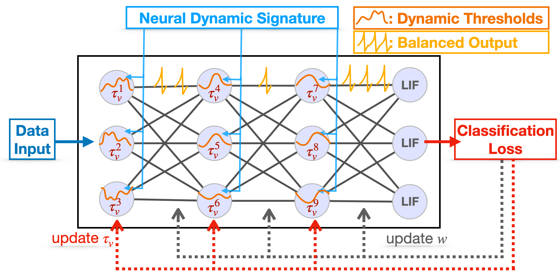
Figure 2: Illustration of the HoSNN

Homeostatic SNNs (HoSNNs)

We introduce the homeostatic SNNs (HoSNNs), which deploy TA-LIF neurons as the basic compute units to leverage their noise immunity as shown in Figure 2. Architecturally, HoSNNs can be constructed by adopting typical connectivity such as feedforward dense or convolutional layers.

In addition to synaptic weights $\bm{\theta}$, the learnable parameters of a HoSNN also include a time-invariant distinct $\tau_{v}$ for each neuron, which specifies the dynamics of the time-varying firing threshold per (25). Given the NDS $\mathcal{A}_{\text{NET}}(\bm{\theta}^{*},\mathcal{D})$ defined in (19), the HoSNN’s optimization problem can be described as:

$$\underset{\bm{\theta},\bm{\tau}_{v}}{\text{min}}\ \mathbb{E}_{(\mathit{x},\mathit{y})\sim\mathcal{T}}[\mathcal{L}\left(\mathit{y},f\left(\mathit{x};\bm{\theta},\bm{\tau}_{v}|\mathcal{A}_{\text{NET}}(\bm{\theta}^{*},\mathcal{D})\right)\right)]$$ (15)

where $\mathit{x}$ and $\mathit{y}$ are an input/label pair sampled from a training distribution $\mathcal{T}$, $f(x)$ is the HoSNN output, $\mathcal{L}(y,f(x))$ is the training loss. In practice, the training data can be chosen to include the clean dataset, an adversarial example dataset, or a combination of the two.

The network-level NDS $\mathcal{A}_{\text{NET}}$, acting as anchor signals for all TA-LIF neurons, is acquired from a separately well-trained LIF based SNN with the same architecture on $\mathcal{D}$ to capture the semantic information.

In principle, a backpropagation based training algorithm such as BPTT (Neftci, Mostafa, and Zenke 2019; Wu et al. 2018), BPTR (Lee et al. 2020), or TSSL-BP (Zhang and Li 2020) can be applied to optimize the network based on (15), during which each $\tau_{v}$ is constrained to be non-negative. Optimizing the firing threshold time constants $\bm{\tau_{v}}$ of all TA-LIF neurons adds insignificant overhead given the dominance of the weight parameter count.

Experiments

In this section, we compare the adversarial robustness of HoSNN with traditional LIF SNN. We train both networks on the original dataset and on the low-intensity fgsm adversarial training respectively, and evaluate their robustness. The former evaluates the intrinsic robustness of the network, and the latter evaluates the transferability and scalability after adversarial training. We further conduct an ablation study on the key parameter $\tau_{v}$ to clarify the underlying mechanism of HoSNN.

Experimental Setup

We evaluated our approach across three benchmark datasets: MNIST (LeCun, Cortes, and Burges 1998), CIFAR10 and CIFAR100 (Krizhevsky 2009). For our experiments, we use LeNet (LeCun et al. 1998) for MNIST, and VGG9-like (Simonyan and Zisserman 2015) architectures for CIFAR10 and CIFAR100.

For robustness assessment, we incorporated different attack methodologies, including FGSM, RFGSM, PGD, and BIM. The key parameters for these attacks are as follows: for both CIFAR10 and CIFAR100, the attack budget is set to $\epsilon=8/255$. For iterative attacks such as PGD, we adopted parameters $\alpha=0.01$ and $steps=7$, in accordance with (Ding et al. 2022). Regarding adversarial training, we use FGSM adversarial training with $\epsilon$ of 2/255 on CIFAR10 as (Ding et al. 2022) and 4/255 on CIFAR100 as (Kundu, Pedram, and Beerel 2021).

For all HoSNN experiments, we initially trained an LIF SNN with an identical architecture on the corresponding clean dataset to derive the NDS. Both HoSNN and SNN employed the BPTT learning algorithm ($T=5$), leveraging a sigmoid surrogate gradient (Xu et al. 2022; Neftci, Mostafa, and Zenke 2019; Wu et al. 2018). The learning rate for $\tau_{v}$ was set at 1/10 of the learning rate designated for weights, ensuring hyperparameter stability during training. Additionally, we ensured $\tau_{v}$ is non-negative during optimization to allow degradation from TA-LIF to LIF. For brevity, in all tables, HoSNNs are labeled as “Ho”, adversarial training as “Adv”, CIFAR-10 as “C-10”, and CIFAR-100 as “C-100”. Comprehensive settings are detailed in the appendix.

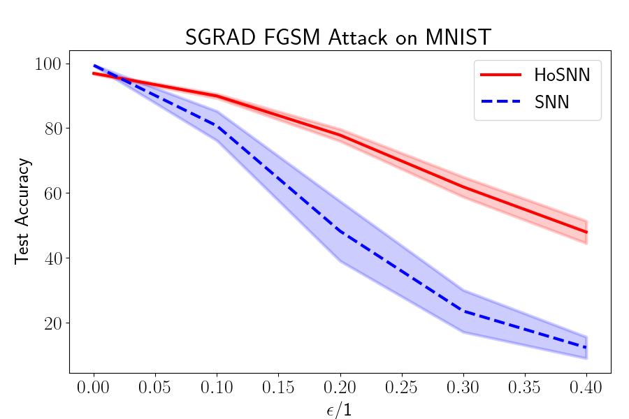
(a) FGSM Attack

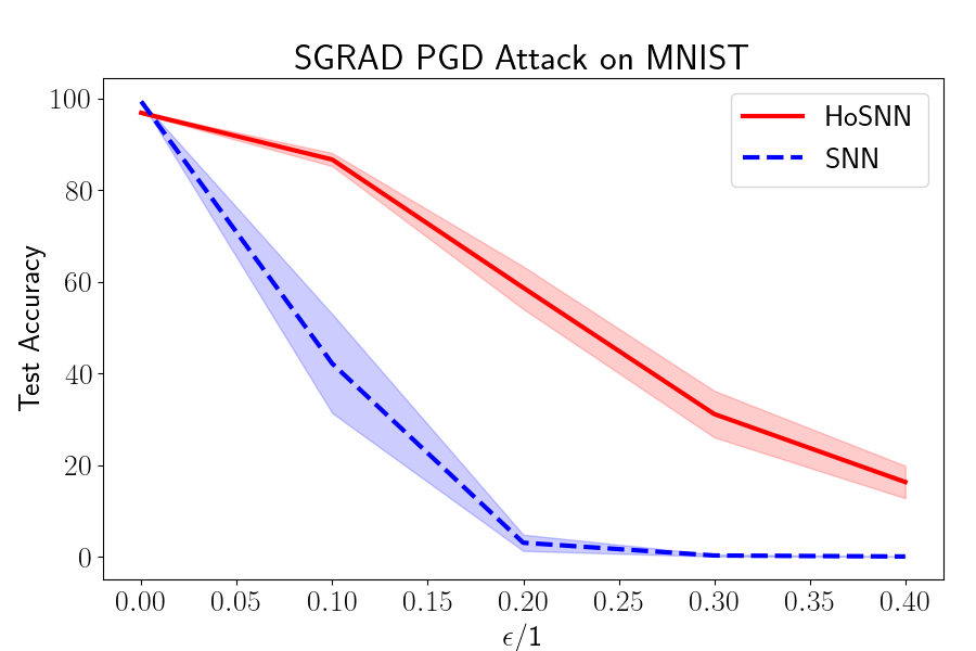
(b) PGD Attack

Figure 3: Attack results on MNIST. The blue dashed line shows the result of training the SNN using the original MNIST dataset, and the red solid line shows the result of the HoSNN. We show the mean and standard deviation of ten experiments.

Data	Ho	Adv	Clean	FGSM	RFGSM	PGD	BIM
C- 10	$\times$	$\times$	92.46	20.97	38.94	0.6	3.29
	$\checkmark$	$\times$	91.62	$\mathbf{72.60}$	$\mathbf{74.90}$	$\mathbf{54.19}$	$\mathbf{64.46}$
	$\times$	$\checkmark$	91.85	38.04	58.98	11.85	22.19
	$\checkmark$	$\checkmark$	90.30	$\mathbf{75.22}$	$\mathbf{77.99}$	$\mathbf{68.99}$	$\mathbf{71.21}$
C- 100	$\times$	$\times$	74.00	5.74	8.94	0.04	0.10
	$\checkmark$	$\times$	70.14	9.30	16.77	0.55	1.52
	$\times$	$\checkmark$	68.72	22.54	36.93	8.82	13.58
	$\checkmark$	$\checkmark$	65.37	$\mathbf{27.18}$	$\mathbf{45.35}$	$\mathbf{18.47}$	$\mathbf{22.58}$

Table 1: White box attack results on CIFAR10 and CIFAR100. HoSNNs are labeled as “Ho”, adversarial training as “Adv”, CIFAR-10 as “C-10”, CIFAR-100 as “C-100”.

Adversarial Robustness

Inherent Robustness without Adversarial Training

To evaluate the natural resilience of our models, we trained both SNN and HoSNN architectures exclusively on clean datasets, and then subjected them to white-box adversarial testing. Figures 3(a) and 3(b), which present the results on the MNIST, demonstrate that HoSNNs necessitate a higher magnitude of adversarial perturbation to achieve a similar degradation in performance, underscoring their inherent robustness. In Table 1, this observation is further supported by results on the CIFAR-10 (rows 1&2) and CIFAR-100 (rows 5&6), indicating the superior resilience of the TA-LIF mechanism against white-box adversarial assaults. For CIFAR-10, HoSNNs without adversarial training improved the accuracy from 20.97% to 72.60% under FGSM attacks, and from 0.6% to 54.19% under PGD attacks. For CIFAR-100, the gains are similar but more modest. These findings reinforce the notion that HoSNNs, even in the absence of adversarial training, exhibit a notable resistance to white-box adversarial threats, underlining their innate robustness.

Enhanced Robustness with Adversarial Training

To evaluate the combined robustness of HoSNN and adversarial training, we explored their transferability and scalability. We trained both SNN and HoSNN using low-intensity FGSM samples and then exposed them to more complex and larger $\epsilon$ white-box attacks. Results in Table 1 (rows 3 & 4 for CIFAR10 and rows 7 & 8 for CIFAR100) show a significant boost in robustness for HoSNNs when combined with adversarial training. On CIFAR-10, this combination increased robustness for FGSM (to 75.22% from 38.04%) and PGD (to 68.99% from 11.85%), and similarly for RFGSM and BIM. For CIFAR-100, resilience improved against FGSM (to 27.18% from 22.54%) and PGD (to 18.47% from 8.82%). In conclusion, the integration of HoSNN with adversarial training gives it the versatility to withstand a wider range of more powerful adversarial attacks.

Data	Ho	Clean	FGSM	RFGSM	PGD	BIM
C- 10	$\times$	91.85	54.59	72.17	47.08	44.42
	$\checkmark$	90.30	$\mathbf{71.16}$	$\mathbf{81.44}$	$\mathbf{75.00}$	$\mathbf{73.48}$
C- 100	$\times$	68.72	47.49	57.96	50.25	51.77
	$\checkmark$	65.37	$\mathbf{52.32}$	$\mathbf{58.98}$	$\mathbf{54.19}$	$\mathbf{55.01}$

Table 2: Black box attack results of SNN and HoSNNs

Data	BPTT Attack	Clean	FGSM	PGD
C- 10	Sharmin et al. [2020]	89.30	15.00	3.80
	Kundu et al. [2021]	87.50	38.00	9.10
	Ding et al. [2022]	90.74	45.23	21.16
	Our work(w/o adv)	$\mathbf{91.62}$	$\mathbf{72.60}$	$\mathbf{54.19}$
	Our work(with adv)	90.30	$\mathbf{75.22}$	$\mathbf{68.99}$
C- 100	Sharmin et al. [2020]	64.40	15.50	6.30
	Kundu et al. [2021]	65.10	22.00	7.50
	Ding et al. [2022]	70.89	25.86	10.38
	Our work(with adv)	65.37	$\mathbf{27.18}$	$\mathbf{18.47}$

Table 3: Comparison with others work

Black Box Attack

In this section, we evaluate the robustness of HoSNN against black-box attacks. Both SNN and HoSNN are trained using low-intensity FGSM adversarial training. We employ a separately trained SNN with an identical architecture to generate white-box attack samples. The results in Table 2 shows for the CIFAR-10, when trained with low-strength FGSM, HoSNNs exhibit significant resistance against adversarial attacks, outperforming the traditional SNNs in FGSM and PGD scenarios with improvements of 16.57% and 27.92% respectively. Likewise, on CIFAR-100, HoSNN shows a similar but weaker robustness improvement. Such robustness underscores the effective incorporation of the homeostatic mechanism into SNNs, making them considerably more robust against adversarial intrusions in black-box scenarios.

Comparison with Other Works

To assess the effectiveness of our method, we compare it against recent state-of-the-art approaches datasets under white box FGSM and PGD attacks on CIFAR-10 and CIFAR-100 in Table 3. Remarkably, even without adversarial training, our method achieved a clean accuracy of $91.62\%$, FGSM defense accuracy of $72.60\%$, and PGD defense accuracy of $54.19\%$ on CIFAR-10. These results surpass those of other methods that employ adversarial training. With adversarial training incorporated, our model further enhanced its robustness. Especially on CIFAR-100, our adversarially trained model achieved the highest defense accuracies of $27.18\%$ and $18.47\%$ for FGSM and PGD, respectively.

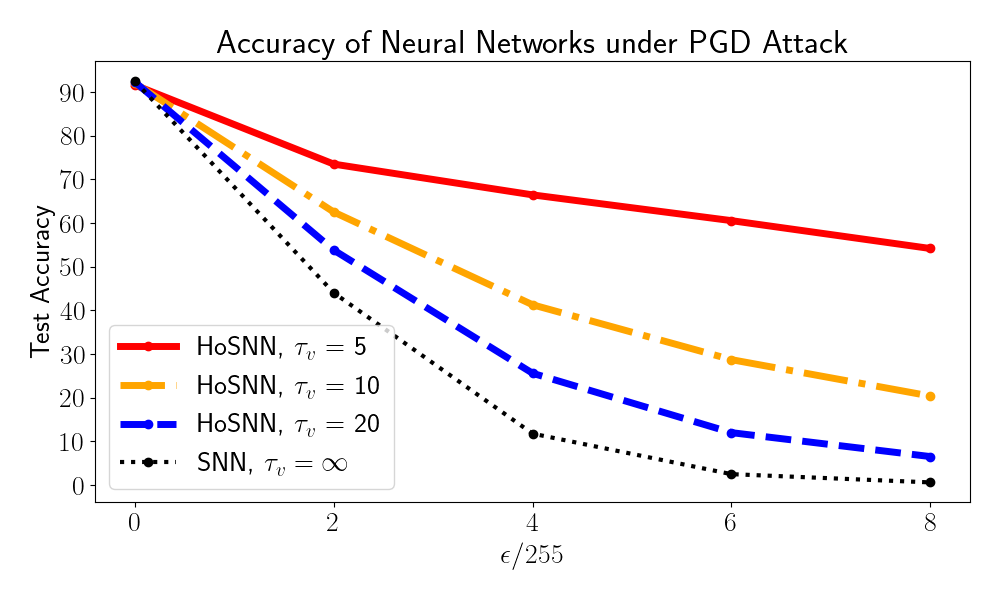
(a) $\tau_{v}$’s Effect on Robustness

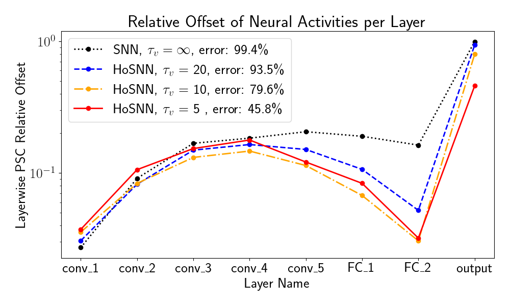
(b) Neural Activity Offset

Figure 4: Network analysis. Three different HoSNNs were trained on CIFAR10 with initial values of $\tau_{v}$ 5, 10, 20 respectively

Ablation studies on $\tau_{v}$

To better understand our model, we conducted a further analysis on $\tau_{v}$. This helps elucidate the distinct features of TA-LIFs and HoSNNs. Figure 4(a) display the accuracy under PGD attacks of three HoSNNs with three distinct initial $\tau_{v}$ values. As anticipated, a smaller initial $\tau_{v}$ value, indicating of greater noise filtering capability, leads to superior adversarial robustness.

To gain insight into the noise suppression mechanism of HoSNNs, we evaluated the offset of each layer’s postsynaptic current (PSC) as illustrated in Figure 4(b). For each neuron $i$ in layer $l$, we computed its mean PSC sequence $\overline{a_{i}(t)}$ using the clean CIFAR10 and its mean PSC under the white-box PGD attack as $\overline{a^{\prime}_{i}(t)}$. The relative offset of layer $l$ can be quantified by: $\frac{\sum_{i,t}|\overline{a_{i}(t)}-\overline{a^{\prime}_{i}(t)}|}{\sum_{i,t}|\overline{a_{i}(t)}|}$

In Figure 4(b), as we expected, standard SNNs under PGD attacks amplify minor perturbations through convolutional layers to fully connected layers, causing output misclassifications. For HoSNN, error signals are magnified in early convolutional layers in a similar magnitude, but as we progress deeper, the TA-LIF’s neuronal activity offset decreases, minimizing by the penultimate layer and reducing classification errors. This behavior aligns with common understanding of CNNs (Zeiler and Fergus 2014): the initial convolutional layers handle low-level features where individual neurons might fail to discern between adversarial noise and standard input. As the depth increases, high-level semantic features emerge, and TA-LIF becomes instrumental in filtering out deviant semantic information. It’s worth noting that while different $\tau_{v}$ values effectively reduce the neuronal activity offset in the penultimate layer, residual perturbations can still convey potent attack information as shown in the curve $\tau^{init}_{v}=20$. This observation is consistent with prior research (Ilyas et al. 2019), which posits that certain adversarial signals, termed “non-robust” features, arise from inherent patterns in the data distribution, rendering them challenging to distinguish.

Discussions

Inspired by biological homeostasis, we designed the TA-LIF neuron with a threshold adaptation mechanism and introduced HoSNN, an SNN that is inherently robust and further enhances the effectiveness of adversarial training, achieving state-of-the-art robustness. Yet, we still face challenges with HoSNNs such as increased computational expenses, reduced clean accuracy, and remaining susceptibilities to adversarial attacks. Meanwhile, we recognize the vast, yet untapped, potential of biological homeostasis in neural network research. In particular, the relationship between the properties of individual neurons and the overall performance of the network warrants further exploration. While our work paves the way, there is still much territory to be explored.

Appendix

We mainly present the derivation of the second-order dynamic equation of TA-LIF, the detailed experimental setup and more data in the supplementary material.

Derivation of TA-LIF Dynamic Equation

In this section, we derive the approximate second-order dynamic equations of the threshold-adapting leaky integrate-and-fire (TA-LIF) neurons and subsequently analyze them.

LIF Dynamics

To facilitate our discussion, let’s commence by presenting the first-order dynamic equations of the LIF neuron $i$ at time $t$:

$$\tau_{m}\frac{du_{i}(t)}{dt}=-u_{i}(t)+I_{i}(t)-\tau_{m}s_{i}(t)V_{th}$$ (16)

The input current is defined as

$$I_{i}(t)=R~{}\sum_{j}w_{ij}a_{j}(t)$$ (17)

The spiking behavior $s_{i}(t)$ is defined as:

$$s_{i}(t)=\begin{cases}+\infty&\text{if }u_{i}(t)\geq V_{th}\\ 0&\text{otherwise}\end{cases}=\sum_{f}\delta(t-t_{i}^{f})$$ (18)

And the post-synaptic current dynamics are given by:

$$\tau_{s}\frac{da_{j}(t)}{dt}=-a_{j}(t)+s_{j}(t)$$ (19)

Where:

• $\tau_{m}$: Represents the membrane time constant.

• $I_{i}(t)$: Denotes the input, which is the summation of the pre-synaptic currents.

• $w_{ij}$: Stands for the synaptic weight from neuron $j$ to neuron $i$.

• $a_{j}(t)$: Refers to the post-synaptic current induced by neuron $j$ at time $t$.

• $V_{th}$: Is the static firing threshold.

• $t_{i}^{f}$: Indicates the $f$-th spike time of neuron $i$.

• $\tau_{s}$: Is the synaptic time constant.

Neural Dynamic Signature

Let’s begin by reviewing the definition of the Neural Dynamic Signature (NDS). Given a data instance $x$ sampled from distribution $\mathcal{D}$, the NDS of neuron $i$, contingent upon network parameters $\theta$ and the training set distribution $\mathcal{D}$, can be represented as a temporal series vector $\bm{\alpha_{i}}(\theta,\mathcal{D})$. Specifically, at time $t$, it holds the value:

$$\bm{\alpha_{i}}(t|\theta,\mathcal{D})\coloneqq\mathbb{E}_{x\sim\mathcal{D}}[u_{i}(t|\theta,x)],\ \text{for }t\in[0,T]$$ (20)

To derive the dynamics of NDS, we start by revisiting Equation (16), rewriting it with respect to $x,\theta$

$$\tau_{m}\frac{du_{i}(t|\theta,x)}{dt}=-u_{i}(t|\theta,x)+I_{i}(t|\theta,x)-\tau_{m}s_{i}(t|\theta,x)V_{th}$$ (21)

For the convenience of dynamic analysis, we choose to approximate the discontinuous Dirac function term $s_{i}(t|\theta,x)$ with the average firing rate $r_{i}(\theta,x)$ of neuron $i$. The average firing rate is calculated by

$$r_{i}(\theta,x):=\int_{0}^{T}\frac{s_{i}(t|\theta,x)}{T}dt$$ (22)

This way, they both have the same integral value over time: the number of neuron firings. Substituting Equation (22) into Equation (21) and computing the expectation on both sides, we have:

$$\tau_{m}\mathbb{E}_{x\sim\mathcal{D}}[\frac{du_{i}(t|\theta,x)}{dt}]=-\mathbb{E}_{x\sim\mathcal{D}}[u_{i}(t|\theta,x)]+\mathbb{E}_{x\sim\mathcal{D}}[I_{i}(t|\theta,x)]-\tau_{m}\mathbb{E}_{x\sim\mathcal{D}}[r_{i}(\theta,x)]V_{th}$$ (23)

Here, we denote the average input current of neuron $i$ over the entire dataset as:

$$I^{*}_{i}(t|\theta,\mathcal{D})\coloneqq\mathbb{E}_{x\sim\mathcal{D}}[I_{i}(t|\theta,x)]$$ (24)

and the average spike frequency of neuron $i$ over the entire dataset as:

$$r^{*}_{i}(\theta,\mathcal{D})\coloneqq\mathbb{E}_{x\sim\mathcal{D}}[r_{i}(\theta,x)]$$ (25)

With the definition from Equation (20), the dynamics of NDS can be expressed as:

$$\tau_{m}\frac{d\bm{\alpha_{i}}(t|\theta,\mathcal{D})}{dt}=-\bm{\alpha_{i}}(t|\theta,\mathcal{D})+I^{*}_{i}(t|\theta,\mathcal{D})-\tau_{m}r^{*}_{i}(\theta,\mathcal{D})V_{th}$$ (26)

As mentioned in the main text, we usually expect NDS to have precise semantic information of the distribution $\mathcal{D}$. So NDS should be obtained through a well-trained model with optimal weight parameter $\theta^{*}$ . For clarity in the following sections, we use $\theta^{*}$ to represent the actually used NDS:

$$\tau_{m}\frac{d\bm{\alpha_{i}}(t|\theta^{*},\mathcal{D})}{dt}=-\bm{\alpha_{i}}(t|\theta^{*},\mathcal{D})+I^{*}_{i}(t|\theta^{*},\mathcal{D})-\tau_{m}r^{*}_{i}(\theta^{*},\mathcal{D})V_{th}$$ (27)

TA-LIF Dynamics

In this section, we delve deeper into the dynamical equations governing the TA-LIF neuron and derive its second-order dynamic equation

$$\tau_{m}\frac{du_{i}(t)}{dt}=-u_{i}(t)+I_{i}(t)-\tau_{m}s_{i}(t)V^{i}_{th}(t)$$ (28)

The synaptic input $I_{i}(t)$, the spike generation function $s_{i}(t)$ and post-synaptic current dynamics of TA-LIF are defined same as (17)(18)(19). For a specific network parameter $\theta$ and a sample $x^{\prime}$ drawn from $\mathcal{D^{\prime}}$, the dynamic equation governing the threshold $V^{i}_{th}(t)$ is:

$$\tau_{v}^{i}\frac{dV_{th}^{i}(t|\theta,x^{\prime})}{dt}=e_{i}(t|\theta,x^{\prime}),$$ (29)

where the error signal, utilizing the NDS as given in (20), is defined as:

$$e_{i}(t|\theta,x^{\prime})\coloneqq u_{i}(t|\theta,x^{\prime})-\bm{\alpha_{i}}(t|\theta^{*},\mathcal{D})$$ (30)

Applying the continuity approximation for the Dirac function as per (22) and incorporating the conditional dependency of $\theta$ and $x^{\prime}$, rewriting the dynamics for TA-LIF (28) as:

$$\tau_{m}\frac{du_{i}(t|\theta,x^{\prime})}{dt}=-u_{i}(t|\theta,x^{\prime})+I_{i}(t|\theta,x^{\prime})-\tau_{m}r_{i}(\theta,x^{\prime})V^{i}_{th}(t|\theta,x^{\prime})$$ (31)

Subtracting (27) from (31) and employing (30), and denoting

$$\Delta I_{i}(t|\theta,x^{\prime})\coloneqq I_{i}(t|\theta,x^{\prime})-I_{i}^{*}(t|\theta^{*},\mathcal{D})$$ (32)

we derive:

$$\tau_{m}\frac{de_{i}(t|\theta,x^{\prime})}{dt}=-e_{i}(t|\theta,x^{\prime})+\Delta I_{i}(t|\theta,x^{\prime})-\tau_{m}[r_{i}(\theta,x^{\prime})V^{i}_{th}(t|\theta,x^{\prime})-r^{*}_{i}(\theta^{*},\mathcal{D})V_{th}]$$ (33)

Differentiating (33) with respect to time and utilizing the threshold dynamics from (30), we obtain:

$$\tau_{m}\frac{d^{2}e_{i}(t|\theta,x^{\prime})}{dt^{2}}=-\frac{de_{i}(t|\theta,x^{\prime})}{dt}+\frac{d\Delta I_{i}(t|\theta,x^{\prime})}{dt}-\frac{\tau_{m}}{\tau_{v}^{i}}r_{i}(\theta,x^{\prime})e_{i}(t|\theta,x^{\prime})$$ (34)

For succinctness, we will omit dependencies on $\theta$ and $x^{\prime}$, resulting in TA-LIF dynamics in the main text (26):

$$\tau_{m}\frac{d^{2}e_{i}(t)}{dt^{2}}+\frac{de_{i}(t)}{dt}+r_{i}\frac{\tau_{m}}{\tau_{v}^{i}}e_{i}(t)=\frac{d\Delta I_{i}(t)}{dt}$$ (35)

For the standard LIF neurons where $\tau^{i}_{v}\rightarrow\infty$, the equation simplifies to:

$$\tau_{m}\frac{d^{2}e_{i}(t)}{dt^{2}}+\frac{de_{i}(t)}{dt}=\frac{d\Delta I_{i}(t)}{dt}$$ (36)

Dynamic Stability Analysis

In this section, we analyze the stability of (35) and (36) to explore the influence of our dynamic threshold mechanism on the noise suppression ability of TA-LIF neuron.

BIBO Stability of Equation (35)

Characteristic Equation: We first show the BIBO (Bounded Input, Bounded Output) stability (Ogata 2010) of TA-LIF neurons based on (35). The characteristic equation of (35) of non-silent ($r_{i}>0$) and non-degenerating ($\tau_{m},\tau^{i}_{v}>0$) TA-LIF neurons are:

$$\tau_{m}s^{2}+s+r_{i}\frac{\tau_{m}}{\tau^{i}_{v}}=0$$ (37)

and its roots are

$$s_{1,2}=\frac{-1\pm\sqrt{\Delta}}{2\tau_{m}},\ \Delta=1-4r_{i}\frac{\tau_{m}^{2}}{\tau^{i}_{v}}$$ (38)

• For $\Delta>0$: Both roots $s_{1,2}$ are real and negative.

• For $\Delta=0$: There’s a single negative real root.

• For $\Delta<0$: Both roots are complex with negative real parts.

For a second-order system to be BIBO, the roots of its characteristic equation must be a negative real or have a negative parts, which is clearly the case for the TA-LIF model under the above three situations, affirming the BIBO stability of (35). The BIBO stability signifies that with the bounded driving input to system (35), the deviation of the TA-LIF neuron’s membrane potential from its targeted NDS is also bounded, demonstrating the well control of the growth of error $e_{i}(t)$.

Stability of Equation (35) Under White Noise

To elucidate the dynamic characteristics of TA-LIF further, we adopt the prevalent method (Abbott and Van Vreeswijk 1993; Brunel 2000; Gerstner et al. 2014; Renart, Brunel, and Wang 2004), approximating $\Delta I(t)$ with a Wiener process. This approximation effectively represents small, independent, and random perturbations. Hence, the driving force in equation (35) $\frac{d\Delta I_{i}(t)}{dt}$ can be modeled by a Gaussian white noise $F(t)$, leading to the well-established Langevin equation in stochastic differential equations theory (Kloeden et al. 1992; Van Kampen 1992; Risken 1996):

$$\frac{d^{2}e_{i}(t)}{dt^{2}}+\frac{1}{\tau_{m}}\frac{de_{i}(t)}{dt}+\frac{r_{i}}{\tau_{v}^{i}}e_{i}(t)=F(t)$$ (39)

Denoting $\langle\cdot\rangle$ as averaging over time, $F(t)$ is a Gaussian white noise with variance $\sigma^{2}$ which satisfies:

$$\left\{\begin{array}[]{ll}\langle F(t)\rangle&=0,\\ \left\langle F\left(t_{1}\right)F\left(t_{2}\right)\right\rangle&=\sigma^{2}\delta\left(t_{1}-t_{2}\right),\\ \left\langle F\left(t_{1}\right)F\left(t_{2}\right)\cdots F\left(t_{2n+1}\right)\right\rangle&=0,\\ \left\langle F\left(t_{1}\right)F\left(t_{2}\right)\cdots F\left(t_{2n}\right)\right\rangle&=\sum_{\text{all pairs }}\left\langle F\left(t_{i}\right)F\left(t_{j}\right)\right\rangle\cdot\left\langle F\left(t_{k}\right)F\left(t_{l}\right)\right\rangle\cdots\end{array}\right.$$ (40)

where the sum has to be taken over all the different ways in which one can divide the $2n$ time points $t_{1}\cdots t_{2n}$ into $n$ pairs. Under this assumption (40), the solution of the Langevin equation(39) is (Uhlenbeck and Ornstein 1930; Wang and Uhlenbeck 1945):

$$\left\langle[\Delta e_{i}(t)]^{2}\right\rangle=\frac{\tau_{m}\tau^{i}_{v}\sigma^{2}}{2r_{i}}\left[1-e^{\frac{-t}{2\tau_{m}}}\left(\cos\left(\omega_{1}t\right)+\frac{\sin\left(\omega_{1}t\right)}{2\omega_{1}\tau_{m}}\right)\right]=O(\sigma^{2})$$ (41)

where $\Delta e_{i}(t)=e_{i}(t)-\langle e_{i}(t)\rangle$ and $\omega_{1}=\sqrt{\frac{r_{i}}{\tau_{v}^{i}}-\frac{1}{4\tau^{2}_{m}}}$. While under the same assumptions (40), equation (36) yields:

$$\left\langle[\Delta e_{i}(t)]^{2}\right\rangle=\frac{\tau_{m}^{2}\sigma^{2}}{2}\left(t-\tau_{m}+\tau_{m}e^{-t/\tau_{m}}\right)=O(\sigma^{2}t)$$ (42)

Obviously, gaussian white noise with zero mean (40) leads $\langle e_{i}(t)\rangle=0$, $\langle[\Delta e_{i}(t)]^{2}\rangle=\langle e_{i}^{2}(t)\rangle$. Hence,

$$\frac{d\Delta I(t)}{dt}\sim F(t)\implies\begin{cases}&\langle e_{i}^{2}(t)\rangle_{LIF}=O(\sigma^{2}t)\\ &\langle e_{i}^{2}(t)\rangle_{TA-LIF}=O(\sigma^{2})\end{cases}$$ (43)

Significantly, the mean square error $\langle e_{i}^{2}(t)\rangle_{TA-LIF}$ of the TA-LIF neuron remains bounded to $O(\sigma^{2})$ and doesn’t increase over time. In contrast, under identical input perturbations, the mean square error $\langle e_{i}^{2}(t)\rangle_{LIF}$ of the LIF neuron may grow unbounded with time, highlighting its potential susceptibility to adversarial attacks.

Experiment Setting Details

Our evaluation encompasses three benchmark datasets: MNIST, CIFAR10, and CIFAR100. For experimental setups, we deploy:

• LeNet (15C5-P-40C5-P-300) for MNIST.

• VGGs (128C3-P-256C3-P-512C3-1024C3-512C3-1024-512) for CIFAR10 and (128C3-P-256C3-P-512C3-1024C3-512C3-1024-1024) for CIFAR100.

Here, the notation 15C3 represents a convolutional layer with 15 filters of size $5\times 5$, and P stands for a pooling layer using $2\times 2$ filters. For the CIFAR10 and CIFAR100 datasets, we incorporated Batch normalization layers and dropout mechanisms to mitigate overfitting and elevate the performance of the deep networks. In our experiments with MNIST and CIFAR10, the output spike train of LIF neurons was retained to compute the kernel loss, as described in (Zhang and Li 2020). For CIFAR100, we directly employed softmax for performance.

We utilized the Adam optimizer with hyperparameters betas set to (0.9, 0.999), and the $lr=5\times 10^{-4}$ with cosine annealing learning rate scheduler($T=$ epochs). We set batch size to 64 and trained for 200 epochs. All images were transformed into currents to serve as network input. Our code is adapted from (Zhang and Li 2020).

For all HoSNN experiments, a preliminary training phase was carried out using an LIF SNN, sharing the same architecture, on the clean datasets to deduce the NDS. Hyperparameters for LIF and TA-LIF neurons included a simulation time $T=5$ , a Membrane Voltage Constant $\tau_{m}=5$, and a Synapse Constant $\tau_{s}=3$. For the TA-LIF results in the main text, we assigned $\tau_{v}$ initialization values of 1.5, 5, and 5 for MNIST, CIFAR10, and CIFAR100, respectively. All neurons began with an initial threshold of 1. The step function was approximated using $\sigma(x)=\frac{1}{1+e^{-5x}}$, and the BPTT learning algorithm was employed. For TA-ALIF neurons, the learning rate for $\tau_{v}$ was set at a tenth of the rate designated for weights, ensuring hyperparameter stability during training. We also constrained $\tau_{v}$ to remain non-negative during optimization, ensuring a possible transition from TA-LIF to LIF.

Regarding adversarial attack, we use an array of attack strategies, including FGSM, RFGSM, PGD, and BIM. For both CIFAR10 and CIFAR100, we allocated an attack budget with $\epsilon=8/255$. For iterative schemes like PGD, we set $\alpha=0.01$ and $steps=7$, aligning with the recommendations in (Ding et al. 2022). For the adversarial training phase, FGSM training was used with $\epsilon$ values of 2/255 for CIFAR10 (as per (Ding et al. 2022)) and 4/255 for CIFAR100, following (Kundu, Pedram, and Beerel 2021).

Supplementary Data

In this supplementary section, we present additional results on the clean CIFAR10 and CIFAR100 datasets to further elucidate the inherent robustness of HoSNNs, as illustrated in Figures 5(a) and 5(b). For both datasets, three distinct HoSNNs were trained separately, each initialized with different values of $\tau_{v}$. Their performance is then compared with the LIF SNN model when subjected to white-box PGD attacks. The parameters for the PGD attack are the same as those described in the main manuscript, with an iteration step of 7 and $\alpha=\epsilon/3$. Our findings highlight that HoSNNs require a considerably higher perturbation budget to induce a performance drop similar to that observed in LIF SNNs. For instance, on the CIFAR10 dataset, a PGD attack with $\epsilon=8/255$ reduces the LIF SNN’s classification accuracy to virtually zero. In contrast, the HoSNN retains a classification accuracy of up to 54.19%. Similarly, for the CIFAR100 dataset, a PGD attack with $\epsilon=2/255$ results in a meager accuracy of 11.62% for the LIF SNN, while the HoSNN achieves an accuracy of up to 36.89%.

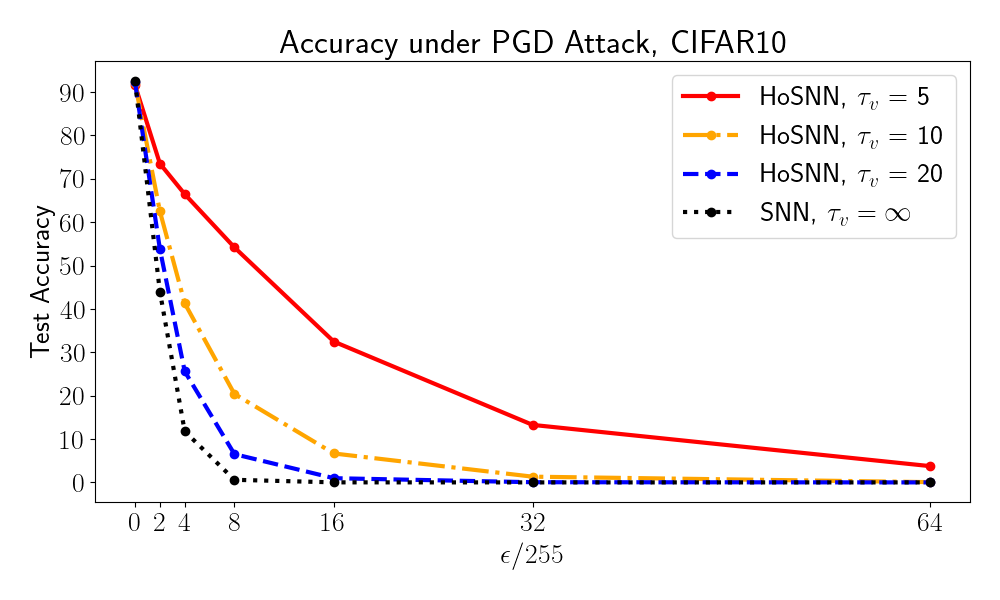
(a) PGD Attack on CIFAR10

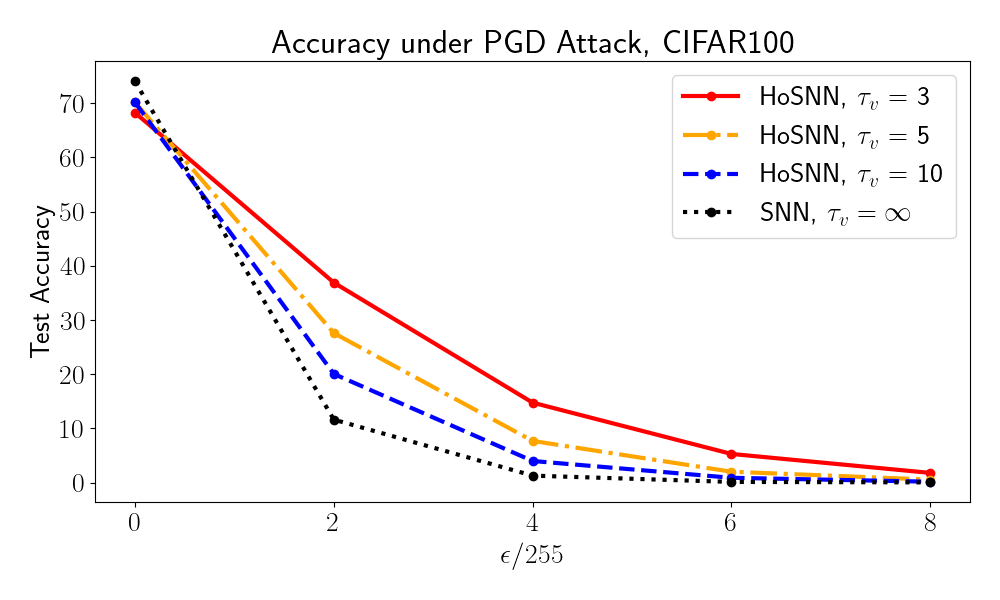
(b) PGD Attack on CIFAR100

Figure 5: More HoSNNs data on CIFAR10 and CIFAR100 under white-box PGD attacks. For the PGD attack, we use an iteration step of 7 and set $\alpha$ to $\epsilon/3$. Our findings highlight that HoSNNs require a considerably higher perturbation budget to induce a performance drop similar to that observed in LIF SNNs.

References

- Abbott and Van Vreeswijk (1993) Abbott, L. F.; and Van Vreeswijk, C. 1993. Asynchronous states in networks of pulse-coupled oscillators. Physical Review E, 48(2): 1483.
- Akhtar and Mian (2018) Akhtar, N.; and Mian, A. 2018. Threat of adversarial attacks on deep learning in computer vision: A survey. Ieee Access, 6: 14410–14430.
- AllenInstitute (2018) AllenInstitute. 2018. Allen Cell Types Database, cell feature search. AllenInstitute.
- Bellec et al. (2018) Bellec, G.; Salaj, D.; Subramoney, A.; Legenstein, R.; and Maass, W. 2018. Long short-term memory and learning-to-learn in networks of spiking neurons. Advances in neural information processing systems, 31.
- Bellec et al. (2020) Bellec, G.; Scherr, F.; Subramoney, A.; Hajek, E.; Salaj, D.; Legenstein, R.; and Maass, W. 2020. A solution to the learning dilemma for recurrent networks of spiking neurons. Nature communications, 11(1): 3625.
- Biggio and Roli (2018) Biggio, B.; and Roli, F. 2018. Wild patterns: Ten years after the rise of adversarial machine learning. In Proceedings of the 2018 ACM SIGSAC Conference on Computer and Communications Security, 2154–2156.
- Bills et al. (2023) Bills, S.; Cammarata, N.; Mossing, D.; Tillman, H.; Gao, L.; Goh, G.; Sutskever, I.; Leike, J.; Wu, J.; and Saunders, W. 2023. Language models can explain neurons in language models. https://openaipublic.blob.core.windows.net/neuron-explainer/paper/index.html.
- Brunel (2000) Brunel, N. 2000. Dynamics of sparsely connected networks of excitatory and inhibitory spiking neurons. Journal of computational neuroscience, 8: 183–208.
- Chowdhury, Lee, and Roy (2021) Chowdhury, S. S.; Lee, C.; and Roy, K. 2021. Towards understanding the effect of leak in spiking neural networks. Neurocomputing, 464: 83–94.
- Davies et al. (2018) Davies, M.; Srinivasa, N.; Lin, T.-H.; Chinya, G.; Cao, Y.; Choday, S. H.; Dimou, G.; Joshi, P.; Imam, N.; Jain, S.; et al. 2018. Loihi: A neuromorphic manycore processor with on-chip learning. Ieee Micro, 38(1): 82–99.
- Ding et al. (2022) Ding, J.; Bu, T.; Yu, Z.; Huang, T.; and Liu, J. 2022. Snn-rat: Robustness-enhanced spiking neural network through regularized adversarial training. Advances in Neural Information Processing Systems, 35: 24780–24793.
- El-Allami et al. (2021) El-Allami, R.; Marchisio, A.; Shafique, M.; and Alouani, I. 2021. Securing deep spiking neural networks against adversarial attacks through inherent structural parameters. In 2021 Design, Automation & Test in Europe Conference & Exhibition (DATE), 774–779. IEEE.
- Fawzi, Moosavi-Dezfooli, and Frossard (2016) Fawzi, A.; Moosavi-Dezfooli, S.-M.; and Frossard, P. 2016. Robustness of classifiers: from adversarial to random noise. Advances in neural information processing systems, 29.
- Ford et al. (2019) Ford, N.; Gilmer, J.; Carlini, N.; and Cubuk, D. 2019. Adversarial examples are a natural consequence of test error in noise. arXiv preprint arXiv:1901.10513.
- Furber et al. (2014) Furber, S. B.; Galluppi, F.; Temple, S.; and Plana, L. A. 2014. The spinnaker project. Proceedings of the IEEE, 102(5): 652–665.
- Gerstner and Kistler (2002) Gerstner, W.; and Kistler, W. M. 2002. Spiking neuron models: Single neurons, populations, plasticity. Cambridge university press.
- Gerstner et al. (2014) Gerstner, W.; Kistler, W. M.; Naud, R.; and Paninski, L. 2014. Neuronal dynamics: From single neurons to networks and models of cognition. Cambridge University Press.
- Goodfellow, Shlens, and Szegedy (2014) Goodfellow, I. J.; Shlens, J.; and Szegedy, C. 2014. Explaining and harnessing adversarial examples. arXiv preprint arXiv:1412.6572.
- Ilyas et al. (2019) Ilyas, A.; Santurkar, S.; Tsipras, D.; Engstrom, L.; Tran, B.; and Madry, A. 2019. Adversarial examples are not bugs, they are features. Advances in neural information processing systems, 32.
- Imam and Cleland (2020) Imam, N.; and Cleland, T. A. 2020. Rapid online learning and robust recall in a neuromorphic olfactory circuit. Nature Machine Intelligence, 2(3): 181–191.
- Kang et al. (2019) Kang, D.; Sun, Y.; Hendrycks, D.; Brown, T.; and Steinhardt, J. 2019. Testing robustness against unforeseen adversaries. arXiv preprint arXiv:1908.08016.
- Kloeden et al. (1992) Kloeden, P. E.; Platen, E.; Kloeden, P. E.; and Platen, E. 1992. Stochastic differential equations. Springer.
- Krizhevsky (2009) Krizhevsky, A. 2009. Learning multiple layers of features from tiny images. Technical report, Citeseer.
- Kundu, Pedram, and Beerel (2021) Kundu, S.; Pedram, M.; and Beerel, P. A. 2021. Hire-snn: Harnessing the inherent robustness of energy-efficient deep spiking neural networks by training with crafted input noise. In Proceedings of the IEEE/CVF International Conference on Computer Vision, 5209–5218.
- Kurakin, Goodfellow, and Bengio (2018) Kurakin, A.; Goodfellow, I. J.; and Bengio, S. 2018. Adversarial examples in the physical world. In Artificial intelligence safety and security, 99–112. Chapman and Hall/CRC.
- LeCun et al. (1998) LeCun, Y.; Bottou, L.; Bengio, Y.; and Haffner, P. 1998. Gradient-based learning applied to document recognition. Proceedings of the IEEE, 86(11): 2278–2324.
- LeCun, Cortes, and Burges (1998) LeCun, Y.; Cortes, C.; and Burges, C. J. 1998. The MNIST database of handwritten digits. ATT Labs [Online]. Available: http://yann.lecun.com/exdb/mnist, 2.
- Lee et al. (2020) Lee, C.; Sarwar, S. S.; Panda, P.; Srinivasan, G.; and Roy, K. 2020. Enabling spike-based backpropagation for training deep neural network architectures. Frontiers in neuroscience, 119.
- Li et al. (2021) Li, T.; Liu, A.; Liu, X.; Xu, Y.; Zhang, C.; and Xie, X. 2021. Understanding adversarial robustness via critical attacking route. Information Sciences, 547: 568–578.
- Li et al. (2022) Li, Y.; Cui, X.; Zhou, Y.; and Li, Y. 2022. A Comparative Study on the Performance and Security Evaluation of Spiking Neural Networks. IEEE Access, 10: 117572–117581.
- Liang et al. (2022) Liang, L.; Xu, K.; Hu, X.; Deng, L.; and Xie, Y. 2022. Toward robust spiking neural network against adversarial perturbation. Advances in Neural Information Processing Systems, 35: 10244–10256.
- Lillicrap et al. (2020) Lillicrap, T. P.; Santoro, A.; Marris, L.; Akerman, C. J.; and Hinton, G. 2020. Backpropagation and the brain. Nature Reviews Neuroscience, 21(6): 335–346.
- Madry et al. (2017) Madry, A.; Makelov, A.; Schmidt, L.; Tsipras, D.; and Vladu, A. 2017. Towards deep learning models resistant to adversarial attacks. arXiv preprint arXiv:1706.06083.
- Marder and Goaillard (2006) Marder, E.; and Goaillard, J.-M. 2006. Variability, compensation and homeostasis in neuron and network function. Nature Reviews Neuroscience, 7(7): 563–574.
- Merolla et al. (2014) Merolla, P. A.; Arthur, J. V.; Alvarez-Icaza, R.; Cassidy, A. S.; Sawada, J.; Akopyan, F.; Jackson, B. L.; Imam, N.; Guo, C.; Nakamura, Y.; et al. 2014. A million spiking-neuron integrated circuit with a scalable communication network and interface. Science, 345(6197): 668–673.
- Metzen et al. (2017) Metzen, J. H.; Genewein, T.; Fischer, V.; and Bischoff, B. 2017. On detecting adversarial perturbations. arXiv preprint arXiv:1702.04267.
- Moosavi-Dezfooli, Fawzi, and Frossard (2016) Moosavi-Dezfooli, S.-M.; Fawzi, A.; and Frossard, P. 2016. Deepfool: a simple and accurate method to fool deep neural networks. In Proceedings of the IEEE conference on computer vision and pattern recognition, 2574–2582.
- Mustafa et al. (2019) Mustafa, A.; Khan, S.; Hayat, M.; Goecke, R.; Shen, J.; and Shao, L. 2019. Adversarial defense by restricting the hidden space of deep neural networks. In Proceedings of the IEEE/CVF International Conference on Computer Vision, 3385–3394.
- Nadhamuni (2021) Nadhamuni, K. 2021. Adversarial Examples and Distribution Shift: A Representations Perspective. Ph.D. thesis, Massachusetts Institute of Technology.
- Neftci, Mostafa, and Zenke (2019) Neftci, E. O.; Mostafa, H.; and Zenke, F. 2019. Surrogate gradient learning in spiking neural networks: Bringing the power of gradient-based optimization to spiking neural networks. IEEE Signal Processing Magazine, 36(6): 51–63.
- Ogata (2010) Ogata, K. 2010. Modern control engineering fifth edition.
- Papernot, McDaniel, and Goodfellow (2016) Papernot, N.; McDaniel, P.; and Goodfellow, I. 2016. Transferability in machine learning: from phenomena to black-box attacks using adversarial samples. arXiv preprint arXiv:1605.07277.
- Pei et al. (2019) Pei, J.; Deng, L.; Song, S.; Zhao, M.; Zhang, Y.; Wu, S.; Wang, G.; Zou, Z.; Wu, Z.; He, W.; et al. 2019. Towards artificial general intelligence with hybrid Tianjic chip architecture. Nature, 572(7767): 106–111.
- Rabanser, Günnemann, and Lipton (2019) Rabanser, S.; Günnemann, S.; and Lipton, Z. 2019. Failing loudly: An empirical study of methods for detecting dataset shift. Advances in Neural Information Processing Systems, 32.
- Renart, Brunel, and Wang (2004) Renart, A.; Brunel, N.; and Wang, X.-J. 2004. Mean-field theory of irregularly spiking neuronal populations and working memory in recurrent cortical networks. Computational neuroscience: A comprehensive approach, 431–490.
- Risken (1996) Risken, H. 1996. The Fokker-Planck Equation: Methods of Solution and Applications. New York: Springer, 2 edition.
- Sharmin et al. (2019) Sharmin, S.; Panda, P.; Sarwar, S. S.; Lee, C.; Ponghiran, W.; and Roy, K. 2019. A comprehensive analysis on adversarial robustness of spiking neural networks. In 2019 International Joint Conference on Neural Networks (IJCNN), 1–8. IEEE.
- Sharmin et al. (2020) Sharmin, S.; Rathi, N.; Panda, P.; and Roy, K. 2020. Inherent adversarial robustness of deep spiking neural networks: Effects of discrete input encoding and non-linear activations. In Computer Vision–ECCV 2020: 16th European Conference, Glasgow, UK, August 23–28, 2020, Proceedings, Part XXIX 16, 399–414. Springer.
- Shu et al. (2020) Shu, M.; Wu, Z.; Goldblum, M.; and Goldstein, T. 2020. Prepare for the worst: Generalizing across domain shifts with adversarial batch normalization.
- Simonyan and Zisserman (2015) Simonyan, K.; and Zisserman, A. 2015. Very deep convolutional networks for large-scale image recognition. In Proceedings of the international conference on learning representations (ICLR).
- Szegedy et al. (2013) Szegedy, C.; Zaremba, W.; Sutskever, I.; Bruna, J.; Erhan, D.; Goodfellow, I.; and Fergus, R. 2013. Intriguing properties of neural networks. arXiv preprint arXiv:1312.6199.
- Tramèr et al. (2017) Tramèr, F.; Kurakin, A.; Papernot, N.; Goodfellow, I.; Boneh, D.; and McDaniel, P. 2017. Ensemble adversarial training: Attacks and defenses. arXiv preprint arXiv:1705.07204.
- Turrigiano and Nelson (2004) Turrigiano, G. G.; and Nelson, S. B. 2004. Homeostatic plasticity in the developing nervous system. Nature reviews neuroscience, 5(2): 97–107.
- Uhlenbeck and Ornstein (1930) Uhlenbeck, G. E.; and Ornstein, L. S. 1930. On the theory of the Brownian motion. Physical review, 36(5): 823.
- Van Kampen (1992) Van Kampen, N. G. 1992. Stochastic processes in physics and chemistry, volume 1. Elsevier.
- Wang and Uhlenbeck (1945) Wang, M. C.; and Uhlenbeck, G. E. 1945. On the theory of the Brownian motion II. Reviews of modern physics, 17(2-3): 323.
- Wu et al. (2018) Wu, Y.; Deng, L.; Li, G.; Zhu, J.; and Shi, L. 2018. Spatio-temporal backpropagation for training high-performance spiking neural networks. Frontiers in neuroscience, 12: 331.
- Xie et al. (2017) Xie, C.; Wang, J.; Zhang, Z.; Ren, Z.; and Yuille, A. 2017. Mitigating adversarial effects through randomization. arXiv preprint arXiv:1711.01991.
- Xu et al. (2022) Xu, N.; Mahmood, K.; Fang, H.; Rathbun, E.; Ding, C.; and Wen, W. 2022. Securing the spike: On the transferabilty and security of spiking neural networks to adversarial examples. arXiv preprint arXiv:2209.03358.
- Zeiler and Fergus (2014) Zeiler, M. D.; and Fergus, R. 2014. Visualizing and understanding convolutional networks. In Computer Vision–ECCV 2014: 13th European Conference, Zurich, Switzerland, September 6-12, 2014, Proceedings, Part I 13, 818–833. Springer.
- Zhang and Li (2020) Zhang, W.; and Li, P. 2020. Temporal spike sequence learning via backpropagation for deep spiking neural networks. Advances in Neural Information Processing Systems, 33: 12022–12033.