Efficient-VRNet: An Exquisite Fusion Network for Riverway Panoptic Perception based on Asymmetric Fair Fusion of Vision and 4D mmWave Radar

Abstract

Panoptic perception is essential to unmanned surface vehicles (USVs) for autonomous navigation. The current panoptic perception scheme is mainly based on vision only, that is, object detection and semantic segmentation are performed simultaneously based on camera sensors. Nevertheless, the fusion of camera and radar sensors is regarded as a promising method which could substitute pure vision methods, but almost all works focus on object detection only. Therefore, how to maximize and subtly fuse the features of vision and radar to improve both detection and segmentation is a challenge. In this paper, we focus on riverway panoptic perception based on USVs, which is a considerably unexplored field compared with road panoptic perception. We propose Efficient-VRNet, a model based on Contextual Clustering (CoC) and the asymmetric fusion of vision and 4D mmWave radar, which treats both vision and radar modalities fairly. Efficient-VRNet can simultaneously perform detection and segmentation of riverway objects and drivable area segmentation. Furthermore, we adopt an uncertainty-based panoptic perception training strategy to train Efficient-VRNet. In the experiments, our Efficient-VRNet achieves better performances on our collected dataset than other uni-modal models, especially in adverse weather and environment with poor lighting conditions. Our code and models are available at https://github.com/GuanRunwei/Efficient-VRNet.

Efficient-VRNet, a robust model for riverway panoptic perception based on the fusion of vision and radar, taking both image and radar point clouds as irregular point sets by contextual clustering and performing nice in various adverse situations.

Asymmetric fair fusion (AFF), a set of cross-attention modules between image features and radar point cloud features.

Homoscedastic-uncertainty-based multi-task training strategy for panoptic perception tasks.

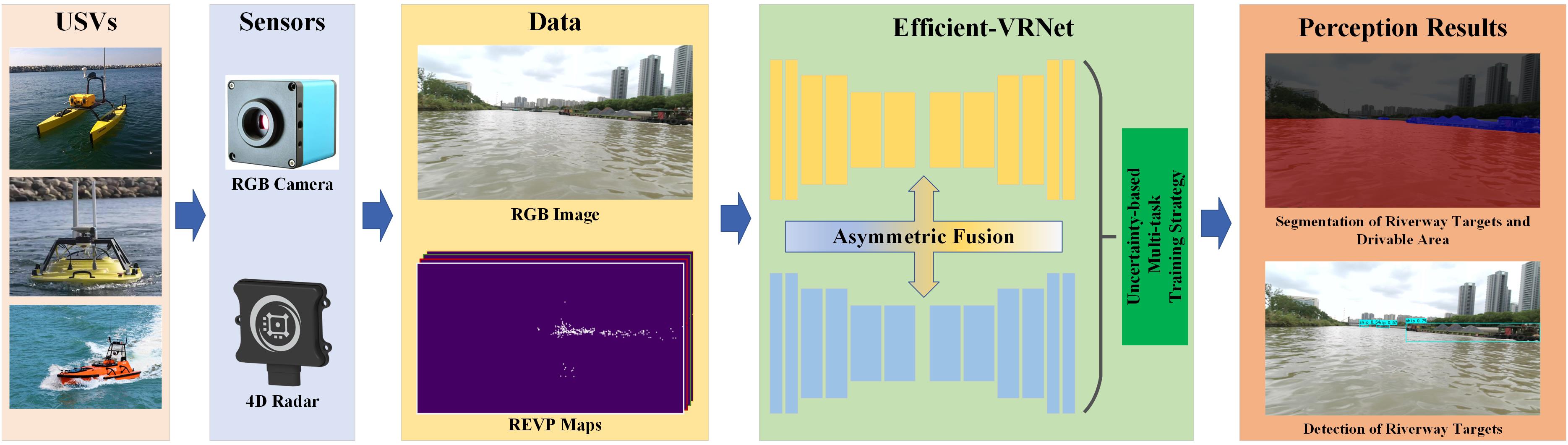
Figure 1: The overview of our proposed methods. It contains five parts, USVs, sensors (monocular camera and 4D radar), data perceived by sensors, Efficient-VRNet, multi-task training strategy and perception results.

1 Introduction

With the rapid development of artificial intelligence and perception sensors, USVs reveal promising values in channel monitoring [27], water-quality monitoring [50], water-surface rescue [42], water-surface transportation [25] and geological prospecting [41]. As one of the essential modules, perception is vital for the autonomous navigation of USVs. Compared to unmanned ground vehicles (UGVs), there is much less research on the perception of USVs, causing slow development. Currently, road-based panoptic perception gradually springs up, which can perform multiple perception tasks (e.g., object detection and semantic segmentation) by one model, friendly to edge devices with limited performance. However, there is no concerned research on water-surface panoptic perception, let alone based on multi-sensor fusion.

Multi-sensor fusion is widely applied to autonomous driving, aiming to make perception more robust than single sensors. However, to our knowledge, most fusion methods are based on camera and lidar. Cameras can capture images with rich features of colour, texture and semantics. Lidar can capture rich point clouds with high resolution. However, both camera and lidar are sensitive to light variation and interference, which perform badly or even fail in adverse weather, hard-light interference and dark environments. Compared with lidar, radar is more robust in adverse environments and has a farther detection range. Nevertheless, point clouds of radar are sparse and lack semantic features. With the development of millimeter wave chip technology, 4D mmWave radar (4D radar), adopting large multiple-input multiple-output (MIMO) antenna arrays, possesses much higher point cloud resolution than ordinary radar and can nicely detect stationary targets. In addition, considering the low cost and small size of 4D radar, the combination of camera and 4D radar is becoming a potential and profound fusion method.

However, based on extensive surveys and experiments, we find that there are considerable limitations and challenges in current methods for riverway panoptic perception.

For exploration degrees of the field,

1. Most current methods are based on vision only [44, 22, 45, 28, 43], which is prone to interference in adverse weather and environments.

2. The current sensor-fusion-based methods for riverway perception focus on object detection only [8, 47]. There are rare researches focusing on panoptic perception tasks.

3. There are rare open-source vision-radar fusion models for 2D perception. It is hard to evaluate their real performances.

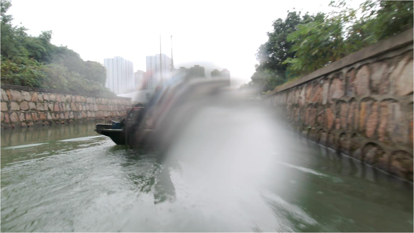
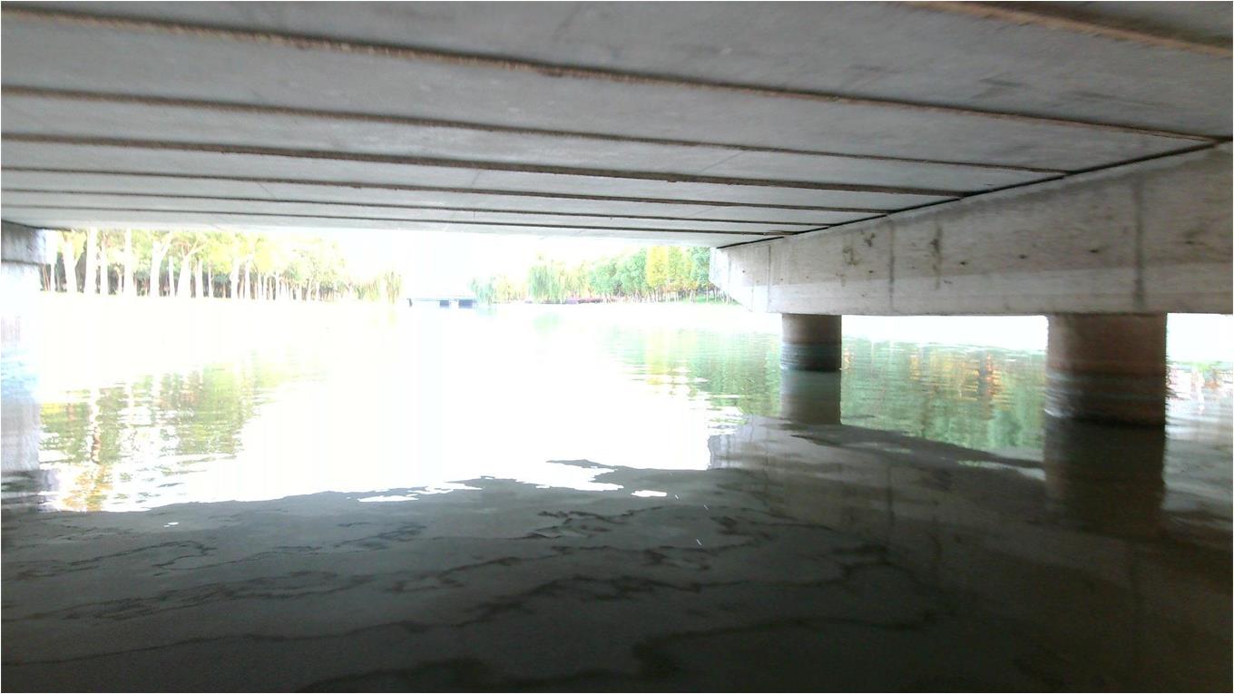
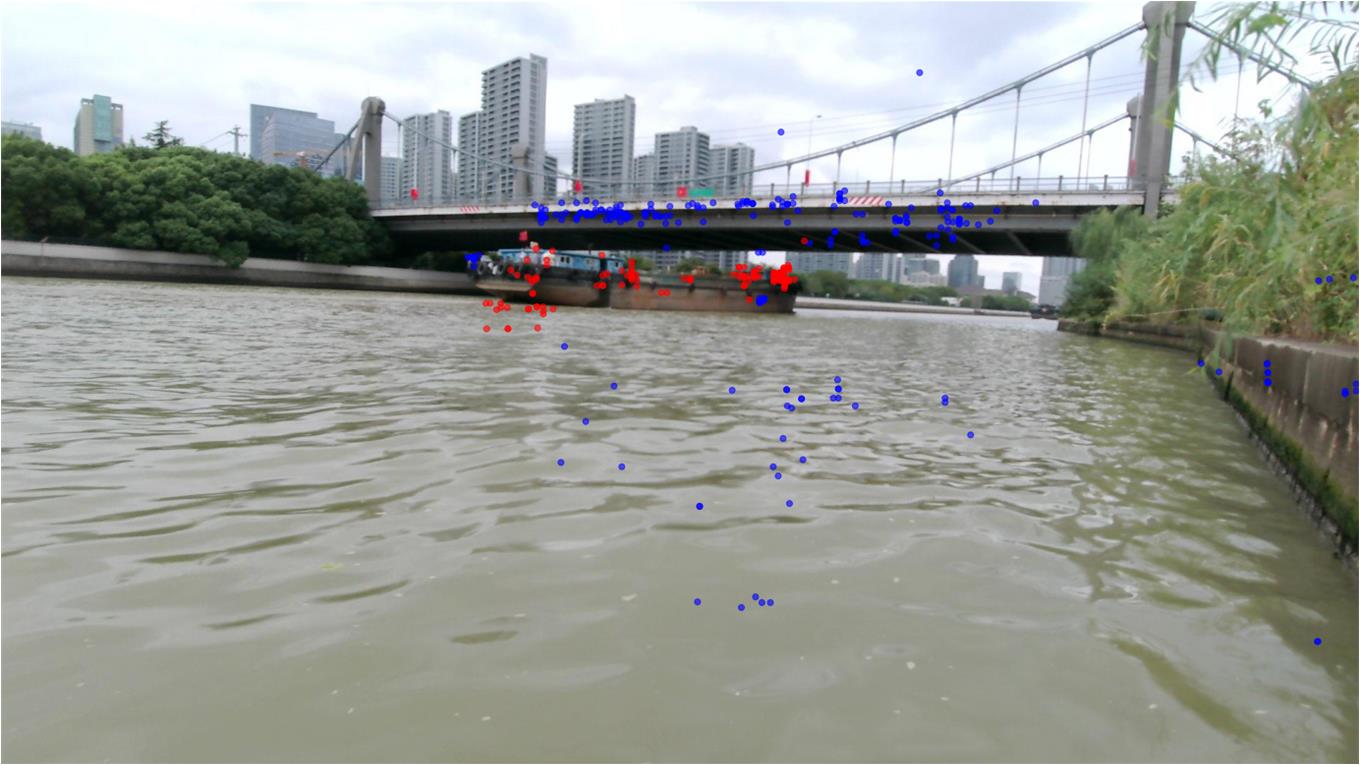
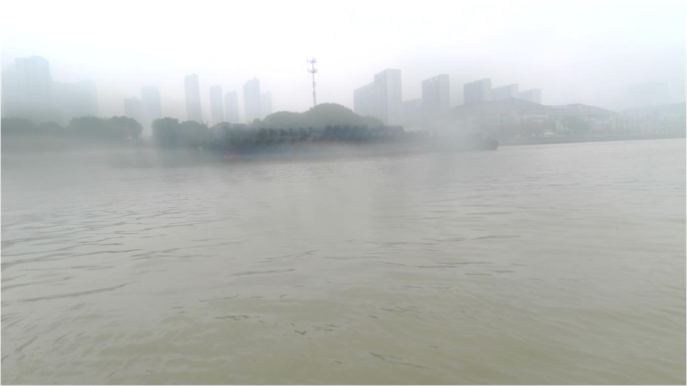
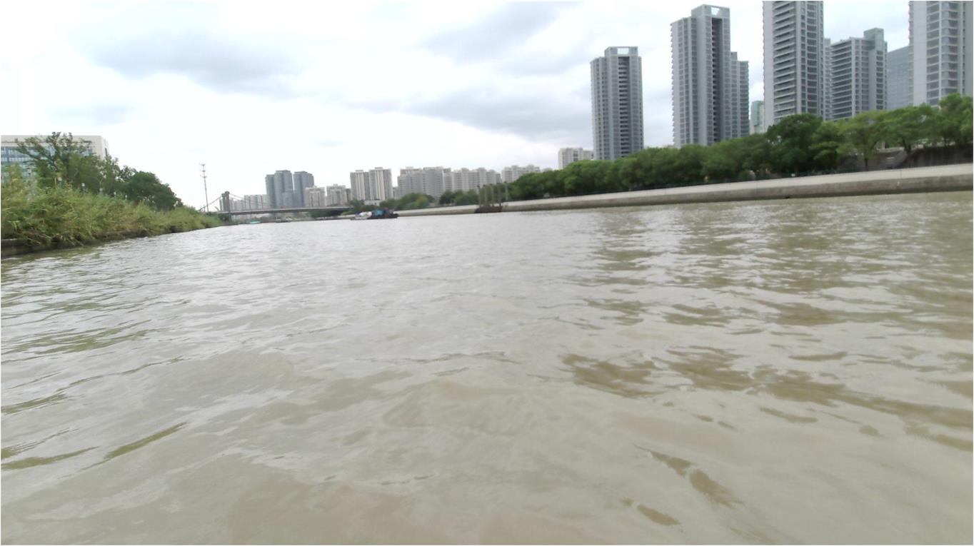
Figure 2: Several challenging scenes in riverway perception based on vision-radar fusion: (a) dark environment, (b) camera malfunction, (c) strong light, (d) radar clutter, (e) adverse weather and (f) small targets.

For sensor performances in riverway perception (Figure 2),

1. Camera is prone to fail when confronted with strong light, adverse weather and dark environments (e.g., underbridge). Furthermore, river water splashing on the lens will cause the camera to malfunction.

2. Although 4D radar is robust in all weather, it still suffers from water-surface clutter.

For feature representations and fusion methods,

1. Almost all vision-radar fusion models are based on convolutional neural networks (CNNs) [8, 17, 16, 29, 21, 34, 32], which use regular rectangle grids to treat irregular targets in images and radar maps.

2. Although many fusion methods are effective [17, 16, 29, 21, 3, 33], they still lack explainability and sufficient validation of effectiveness.

3. Most fusion operations in sensor-fusion models are in the stage of feature extraction (backbone) [17, 16, 29, 21], ignoring the stage of feature fusion (neck).

4. Some works adopt backbones and necks with different structures [8, 48], which would cause features learnt in the backbone to be lost in the neck with different feature representations (e.g., vision transformer as the backbone and CNN-based feature pyramid network (FPN) as the neck).

Based on the above points, we focus on the robust and high-performance riverway panoptic perception. As Figure 1 presents

1. We propose a robust riverway panoptic perception model called Efficient-VRNet. Efficient-VRNet is based on a full contextual-clustering (CoC) [26] structure, including backbone and neck, which takes both image and radar targets as irregular point sets.

2. Based on prior experiments and principle support, we design a set of effective fusion methods for vision-radar fusion, called asymmetric fair fusion (AFF). AFF sufficiently considers the characteristics of different perception tasks and designs the fusion methods according to the features of images and radar maps, which is fair to these two modalities and avoids favouritism. AFF is a fusion method friendly to explainability. Moreover, AFF can perform as the plug-and-play module to insert into any vision-radar fusion network to improve performance.

3. Inspired by homoscedastic uncertainty [18], we design a multi-task training strategy based on the uncertainty of perception tasks during training the panoptic perception model.

2 Related Works

2.1 Panoptic Perception in Autonomous Driving

Panoptic perception is vital in autonomous driving systems no matter for UGVs, USVs or unmanned aerial vehicles (UAVs). The role of panoptic perception models mainly consists of detecting obstacles and segmenting the drivable area. Given the limited computational resources of edge devices, panoptic models combine several perception tasks into one model. YOLOP [39] and YOLOPv2 [14], both based on YOLO-style models, could detect traffic participants, detect lane and segment drivable areas at the same time. HybridNets [35] is a panoptic model adopting EfficientNet [13] as the backbone and combined with an effective multi-task training strategy.

2.2 Water-surface Perception based on Multiple Sensors and USVs

Water-surface perception is an essential part of USVs. Many methods concentrate on the fusion of multiple sensors to complement each other, outperforming the perception ability of a single sensor. Cheng et al. [7] release a multi-sensor simultaneous localization and mapping (SLAM) dataset called USVInland based on a stereo camera, lidar, mmWave radar, GPS and inertial measurement units (IMU). FloW [9] is the first floating waste detection dataset in inland river with camera and radar. Bovcon et al. [2] release a marine semantic segmentation dataset, utilizing cameras, lidar, GPS and IMU. Kim et al. [19] propose a novel data association method for object detection based on marine radar and cameras. Farahnakian et al. [11] propose a two-stage object detection model by fusing the proposals generated by infrared cameras, RGB cameras, lidar and radar. Haghbayan et al. [13] propose a proposal-level fusion method based on probabilistic data association, using infrared cameras, RGB cameras, lidar and radar. Sorial et al. [33] propose a YOLO-based detection and tracking model to detect and track obstacles in maritime environments, utilizing lidar and video camera.

2.3 Simple Linear Iterative Clustering Algorithm and Its Extension

Simple linear iterative clustering (SLIC) algorithm [1] is to generate superpixels with perception meaning by k-means clustering. Superpixel is a substitute for pixel grids with rigid structure. The detailed SLIC algorithm is presented in Algorithm 1. We visualize a sample by SLIC algorithm as Figure 3 shows. Based on SLIC, Ma et al. [26] propose contextual clustering (CoC), an image feature extractor, taking an image as a set of points. CoC shows promising potential and generalization for multi-modal learning based on images and point clouds.

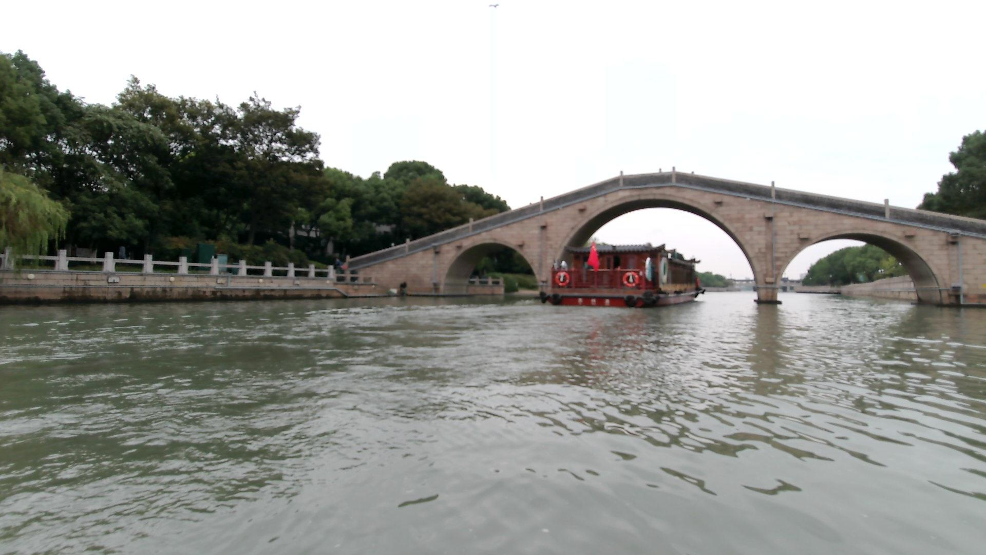
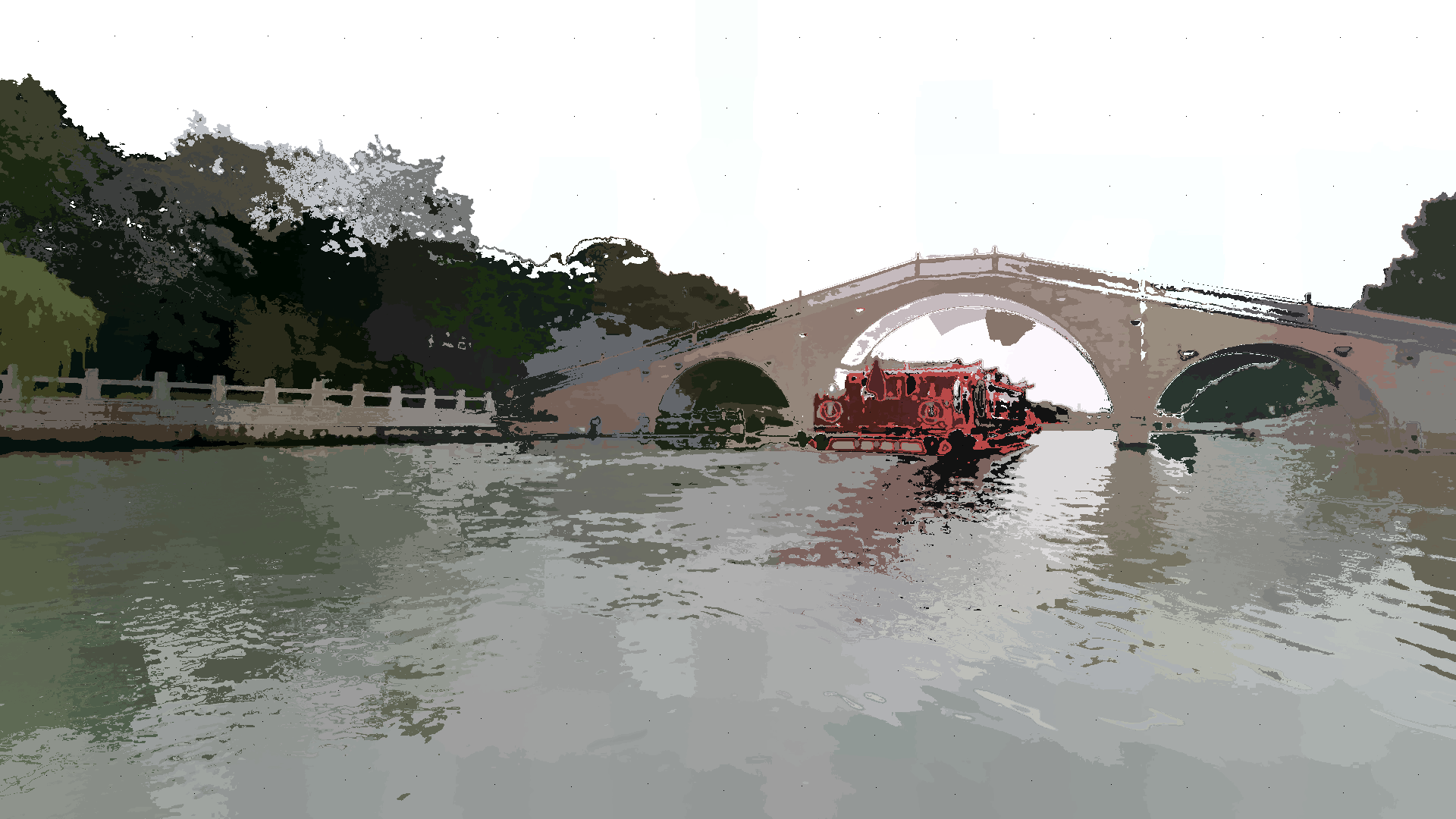
Figure 3: Superpixels generated by SLIC algorithm (b) from the original image (a). Each black point in a superpixel is a clustering center generated by SLIC.

Algorithm 1 SLIC Algorithm

// input and initialize

Input: Image $I$ with $N$ pixels.

Each pixel $P_{i}$ is represented as $P_{i}=[l_{i},a_{i},b_{i},x_{i},y_{i}]^{T}$ in the CIELAB color space.

Sample $k$ centers $C_{k}=[l_{k},a_{k},b_{k},x_{k},y_{k}]^{T}$ at regular steps $S$, $S=\sqrt{\frac{N}{k}}$.

Move $k$ centers to positions with the lowest gradient in the $3\times 3$ neighbourhood.

Define the label of each pixel $i$ as $label(P_{i})=-1$

Define the distance $d(P_{i})=\infty$

Define the threshold of loss $E$ as $TH$

// implement

repeat:

 for each cluster center $C_{k}$ do:

  for each pixel $p_{i}$ in a $2S$ × $2S$ region around $C_{k}$ do:

   Compute the distance $D$ between $C_{k}$ and $P_{i}$.

   if $D$ $<$ $d(P_{i})$ then:

    set $d(P_{i})$ = $D$

    set $l(P_{i})$ = $k$

   end if

  end for

 end for

 Computer new cluster center

 Computer loss $E$

until $E$ $<$ $TH$

2.4 Multi-Task Learning Strategies in Computer Vision

Multi-task learning (MTL) is a classical and challenging problem in deep learning. How to balance the loss of various tasks during the training based on the loss value and characteristics of tasks is an interesting proposition. GradNorm [6] is a classical MTL method, scaling the loss of different tasks into a similar magnitude. Dynamic weight averaging (DWA) [24] is for balancing the learning paces of various tasks. Sener et al. [31] consider MTL as a multiple objective optimization (MOO) problem by finding the Pareto optimal solution among various tasks. Kendall et al. [18] propose an uncertainty-based MTL method, by estimating the weight of various tasks through Gaussian likelihood estimation.

3 Efficient-VRNet

As Figure 4 presents, Efficient-VRNet is a dual-branch model. There are four explicit parts (ep) and one implicit part (ip), perception data (ep), VRCoC (ep), VRCoC-FPN (ep) and Prediction Heads (ep), and asymmetric fair fusion modules (ip). Asymmetric fair fusion modules exist through different stages of Efficient-VRNet.

Figure 4: The architecture of Efficient-VRNet. Efficient-VRNet includes five parts: preprocessing of perception data, VRCoC (backbone), asymmetric fusion modules, VRCoC-FPN (neck) and prediction heads. VRCoC has four stages, where each stage has 2, 2, 6 and 2 layers, respectively.

3.1 Projection of 3D Radar Point Clouds to 2D Image Plane

To establish the relationship between radar point clouds and camera images, we convert radar point clouds from Polar coordinates onto the image plane. Attributes of each radar point include the range, Doppler velocity, azimuth angle, elevation angle, and reflected power. We initially convert radar point clouds from Polar coordinates into Cartesian coordinates $(x,y,z)$ using the values from range $r$, azimuth angle $a$ and elevation angle $e$ according to Equation 1.

$$x=r*\operatorname{sin}(a)*\operatorname{cos}(e)$$ (1)

$$y=r*\operatorname{sin}(e)$$

$$z=r*\operatorname{cos}(a)*\operatorname{cos}(e)$$

Subsequently, we convert the data from Cartesian coordinates to camera coordinates employing the extrinsic matrix $T_{e}$ between the radar sensor and camera sensor. The extrinsic matrix is a 4 $\times$ 4 homogeneous matrix, consisting of a 3 $\times$ 3 rotation matrix $\mathbf{R}$ and a 3 $\times$ 1 translation vector $\mathbf{t}$, as shown in Equation 2. Lastly, the radar point clouds in the camera coordinates are transformed onto the image plane utilizing the intrinsic matrix $T_{i}$ of the camera sensor. The intrinsic matrix is a 3 $\times$ 4 matrix.

$$T_{e}=\begin{bmatrix}\mathbf{R}&\mathbf{t}\\ 0&1\end{bmatrix}$$ (2)

$$X=T_{i}(T_{e}P)$$ (3)

Overall, according to Equation 3, a radar point $P(x,y,z,1)$ on the camera’s image plane in homogeneous coordinates is obtained, represented as $X$, which is a 3 $\times$ 1 matrix. Finally, we can get the 2D coordinates of $P$ on the camera plane from Eq. 4.

$$u=X_{1}/X_{3}$$

$$v=X_{2}/X_{3},$$ (4)

where $X_{1},X_{2},X_{3}$ are the row values in $X$.

3.2 Preprocessing of Perception Data

After projecting the radar point cloud from the radar coordinate to camera coordinate, we choose four radar target features as the representations, which are range, elevation, velocity and power. Firstly, as range and velocity of the target can not been recognized in the dimension of image representation, range and velocity can nicely distinguish targets with different ranges and velocities. Secondly, height gaps between different targets are not evident in many scenarios, but 4D radar can stably obtain height information of targets. Therefore, elevation is also considered as one of representations of targets. Thirdly, compared with the brightness of reflected light of targets in the image, power is a physical quantity that can reasonably measure the radar wave reflection intensity of the target surface, which is not disturbed by the light interference.

Figure 5: The accumulation of radar point clouds at multiple frames in the radar coordinates. Radar point clouds in the red bounding box represent the vessel.

Based on the above, as Figure 4 presents, we concatenate these four feature maps together along the channel dimension and call them REVP map. To improve the density of radar point cloud, we accumulate the radar point clouds of the adjacent four frames, which is shown in Figure 5. It is obvious that the density of radar point clouds is improved notably. However, it is also accompanied by troublesome clutter point clouds. To alleviate the negative impact of clutter, we first exert efficient channel attention (ECA) [38] on the REVP map to calculate the importance degree of radar features, then we put the $1\times 1$ convolution on the REVP map with ECA to pay attention to radar targets and ignore radar clutter adaptively.

3.3 VRCoC

VRCoC, Vision-Radar Contextual Clustering, is the backbone of Efficient-VRNet. As Figure 4 presents, VRCoC is a dual-branch backbone. Each branch is based on contextual clustering to extract the features of RGB image and REVP map, respectively. Given an image $I\in\mathbb{R}^{3\times w\times h}$ and a REVP map $R\in\mathbb{R}^{4\times w\times h}$, we assign the coordinate of each pixel in the RGB image $I_{i,j}$ as $\left[\frac{i}{w}-0.5,\frac{j}{h}-0.5\right]$. Likewise, the coordinate of each element in the REVP map $R_{i,j}$ is assigned as $\left[\frac{i}{w}-0.5,\frac{j}{h}-0.5\right]$. Therefore, the RGB image is transformed into a set of points $IP\in\mathbb{R}^{5\times n}$ while the REVP map is transformed into a set of points $RP\in\mathbb{R}^{6\times n}$, where $n=w\times h$ is the point number of one channel in both RGB image and REVP map. Each point in the RGB image contains the features of color (3 channels) and position (2 channels). For the REVP map, each point includes the physical target features captured by radar (4 channels) and position features (2 channels).

Figure 6: Basic units of VRCoC, including the unit of vision branch and radar branch in VRCoC.

Point Reducer. Based on the sets of points $IP\in\mathbb{R}^{5\times n}$ and $RP\in\mathbb{R}^{6\times n}$ we have got, we start to extract features. As Figure 6 presents, the first step is point reducer, which means reducing the number of points. In this step, following CoC [26], we evenly choose the anchors in the feature space and concatenate the nearest $k$ centers of points, and then a linear feed-forward module is to transform the dimension of feature maps to $d$.

Contextual Clustering. Based on the feature points of the image $IP\in\mathbb{R}^{d\times n}$ and REVP map $RP\in\mathbb{R}^{d\times n}$ in the same stage, we group feature points into several clusters based on the cosine similarity between features of points and features of clustering centers. The clustering centers are evenly selected by SLIC algorithm [1]. After allocating points to respective centers, feature aggregation is applied based on the similarities between clustering points and clustering center. Assuming there are $n$ clustering points in a cluster, the similarity matrix between clustering points and clustering center is $s\in\mathbb{R}^{n}$. Then, we map these feature points into an aggregation space, so $IP\in\mathbb{R}^{d\times n}$ and $RP\in\mathbb{R}^{d\times n}$ are mapped to $IP\in\mathbb{R}^{\hat{d}\times n}$ and $RP\in\mathbb{R}^{\hat{d}\times n}$, respectively, where $\hat{d}$ is the dimension of feature points in the aggregation space. In one cluster in aggregation space, a clustering center $v_{c}$ is proposed based on SLIC algorithm similarly. Therefore, the aggregated feature of points $f\in\mathbb{R}^{\hat{d}\times n}$ is presented in Equation 5,

$$f=\frac{1}{C}\Big{(}v_{c}+\sum\limits_{i=1}^{n}\sigma(\alpha s_{i}+\beta)*v_{i}\Big{)},$$ (5)

$$s.t.,C=1+\sum\limits_{i=1}^{n}\sigma(\alpha s_{i}+\beta).$$

where $\alpha$ and $\beta$ are learnable parameters representing the scale and shift ratio of the similarity. $\sigma$ is the sigmoid function to scale the similarity to $(0,1)$. $v_{i}$ denotes the $i$th points in the aggregation space. $C$ is a normalization factor.

Then the aggregated feature $f$ is dispatched to each feature point in the cluster according to the similarity. For each feature point $p_{i}$, the dispatch step for updating is presented in Equation 6,

$$\hat{p_{i}}=p_{i}+FF\Big{(}\sigma(\alpha s_{i}+\beta)*f\Big{)},\quad\hat{p_{i}}\in\mathbb{R}^{d\times n}.$$ (6)

where $p_{i}$ represents the $i^{th}$ feature point and $\hat{p_{i}}$ represents the updated $i^{th}$ feature point. $\sigma$ is the sigmoid function. $FF$ is the feed-forward module based on fully-connected layers, which transforms the dimension $\hat{d}$ back to $d$.

Based on the above, we get the feature maps of the image $\hat{IP}\in\mathbb{R}^{d\times n}$ and radar $\hat{RP}\in\mathbb{R}^{d\times n}$ updated by the point reducer and contextual clustering in the unit of CoC. Inspired by the multi-head self-attention operation in Vision Transformer [10], we divide the channel of $\hat{IP}$ and $\hat{RP}$ into $h$ parts, and each part denotes one head. Each head $head_{i}$ is weighted individually and concatenated to other heads. After that, we concatenate all heads along the dimension of channels. Multi-head operation can make the network adaptively attach importance to features. The process of the multi-head operation is shown in Equation LABEL:eq:multi-head-coc.

$$\hat{IP}^{{}^{\prime}}=[head^{IP}_{1}W^{IP}_{1},head^{IP}_{2}W^{IP}_{2},\dots,head^{IP}_{h}W^{IP}_{h}],$$ (7)

$$\hat{RP}^{{}^{\prime}}=[head^{RP}_{1}W^{RP}_{1},head^{RP}_{2}W^{RP}_{2},\dots,head^{RP}_{h}W^{RP}_{h}].$$

3.4 AFF-IRC

Figure 7: The architecture of Image-to-Radar Concatenation (IRC).

Figure 8: The comparison result of YOLOv5n with image and with image + REVP on the validation set of our collected dataset.

Motivation. Based on extensive prior experiments on object detection, we find that concatenating the image and REVP map along the channel dimension can dramatically accelerate the convergence of mean average precision ($mAP$). As Figure 8 presents, when the input of YOLOv5n [15] is the concatenation of the image and REVP map, YOLOv5n reaches 80% AP₅₀ about the $50^{th}$ epoch. However, YOLOv5n with the image only reaches 80% $mAP$ about the $70^{th}$ epoch, 20 epochs slower than the former. Furthermore, the concatenation of the image and REVP map make YOLOv5n achieve higher $mAP$ than the image-only YOLOv5n.

From the perspective of object detection, image-based object detection results have no direct causality with the pixel features, which means the brightness or color is not the direct element to locate the target. For instance, the luminous area does not mean that it is the target’s location. Neural network models need to learn from a large number of images to learn the various feature combinations to locate the target. However, 4D radar tremendously improves this situation. 4D radar can capture denser point clouds of targets than ordinary radar, no matter whether the target is moving or still. That is to say, the point cloud of 4D radar can help the neural network model anchor the general area of the target at the beginning of training, thereby speeding up the convergence of object detection. For adverse weather and dark light environments, the point cloud of 4D radar can be used to supplement the lack of visual features, and to a certain extent avoid the missed detection of targets.

Architecture. Based on the above, we propose the module of image-to-radar concatenation (IRC). IRC is a module in asymmetric fair fusion, which is to fuse the features of image and radar in the radar branch for object detection. As Figure 7 presents, assuming a feature map $f^{I}_{i}\in\mathbb{R}^{c\times h\times w}$ in the vision branch and a feature map $f^{R}_{i}\in\mathbb{R}^{c\times h\times w}$ in the radar branch. $f^{I}_{i}$ is firstly divided into $g$ pieces and each piece is $f^{I}_{i_{j}}\in\mathbb{R}^{\frac{c}{g}\times h\times w}$, and then it will be divided in half. The first is spatial attention branch and the second is channel attention branch.

For the channel attention, given the input feature map $f^{I}_{i_{j-c}}\in\mathbb{R}^{\frac{c}{2g}\times h\times w}$, as Equation LABEL:eq:irc-ca presents, $f^{I}_{i_{j-c}}$ is processed by the global average pooling to capture the global representation, then a non-linear and a sigmoid function are exerted to measure the channel importance. Finally, the channel importance is multiplied with the input feature map $f^{I}_{i_{j-c}}$ to obtain the feature map with channel attention $\hat{f}^{I}_{i_{j-c}}\in\mathbb{R}^{\frac{c}{2g}\times h\times w}$.

$$f^{I}_{i_{j-c-1}}=\sigma\Big{(}W_{c}\cdot GP(f^{I}_{i_{j-c}})+b_{c}\Big{)},\quad f^{I}_{i_{j-c-1}}\in\mathbb{R}^{\frac{c}{2g}\times 1\times 1},$$ (8)

$$\hat{f}^{I}_{i_{j-c}}=f^{I}_{i_{j-c-1}}*f^{I}_{i_{j-c}},\quad\hat{f}^{I}_{i_{j-c}}\in\mathbb{R}^{\frac{c}{2g}\times h\times w}.$$

where $GP$ denotes global average pooling. $W_{c}$ is the learnable weight in the non-linear feed-forward module while $b_{c}$ is the learnable bias. $\sigma$ is the sigmoid function. $*$ denotes element-wise multiplication.

For the spatial attention, given the input feature map $f^{I}_{i_{j-s}}\in\mathbb{R}^{\frac{c}{2g}\times h\times w}$, as Equation LABEL:eq:irc-sa presents, $f^{I}_{i_{j-s}}$ is first normalized by group, then processed by a non-linear feed-forward module and a sigmoid function to measure the spatial importance. Finally, the spatial importance is multiplied with the input feature map $f^{I}_{i_{j-s}}$ to obtain the feature map with spatial attention $\hat{f}^{I}_{i_{j-s}}\in\mathbb{R}^{\frac{c}{2g}\times h\times w}$.

$$f^{I}_{i_{j-s-1}}=\sigma\Big{(}W_{s}\cdot GN(f^{I}_{i_{j-s}})+b_{s}\Big{)},\quad f^{I}_{i_{j-s-1}}\in\mathbb{R}^{\frac{c}{2g}\times h\times w},$$ (9)

$$\hat{f}^{I}_{i_{j-s}}=f^{I}_{i_{j-s-1}}*f^{I}_{i_{j-s}},\quad\hat{f}^{I}_{i_{j-s}}\in\mathbb{R}^{\frac{c}{2g}\times h\times w}.$$

where $GN$ denotes group-norm. $W_{s}$ is the learnable weight in the non-linear feed-forward module while $b_{s}$ is the learnable bias. $\sigma$ is the sigmoid function while $*$ denotes element-wise multiplication.

After that, we concatenate $\hat{f}^{I}_{i_{j-s}}$ and $\hat{f}^{I}_{i_{j-c}}$ and get the combination of the feature map $\hat{f}^{I}_{i_{j-sc}}$ with both channel and spatial attention. Aggregation (concatenation) of $g$ $\hat{f}^{I}_{i_{j-sc}}$ is implemented to get the initial feature map with channel and spatial attention $f^{I}_{i_{sc}}\in\mathbb{R}^{c\times h\times w}$. We concatenate $f^{I}_{i_{sc}}$ and $f^{R}_{i}\in\mathbb{R}^{c\times h\times w}$ along the channel dimension (Equation 10).

$$f^{IR}_{i}=[f^{I}_{i_{sc}},f^{R}_{i}],\quad f^{IR}_{i}\in\mathbb{R}^{2c\times h\times w}.$$ (10)

where $[\cdot]$ is the concatenation operation.

After that, the channel shuffle is exerted to enhance the interaction among features, and then we adopt efficient channel attention (ECA) [38] to adaptively weigh the channels, followed by a feed-forward module, reducing the channel dimension. Finally, a long residual path is added and we get the feature map $f^{R}_{i+1}$ updated by IRC in the radar branch. The whole process is shown in Equation LABEL:eq:irc-final-stage.

$$f^{IR-ECA}_{i}=ECA\Big{(}S(f^{IR}_{i})\Big{)},\quad f^{IR-ECA}_{i}\in\mathbb{R}^{2c\times h\times w},$$ (11)

$$\hat{f}^{IR}_{i}=W_{f}\cdot f^{IR-ECA}_{i}+b_{f},\quad\hat{f}^{IR}_{i}\in\mathbb{R}^{c\times h\times w},$$

$$f^{R}_{i+1}=\hat{f}^{IR}_{i}+f^{R}_{i},\quad f^{R}_{i+1}\in\mathbb{R}^{c\times h\times w}.$$

where $S(\cdot)$ denotes the channel shuffle. $W_{f}$ is the learnable weight in the non-linear feed-forward module while $b_{f}$ is the learnable bias.

3.5 AFF-RIM

Motivation. The vision branch is for semantic segmentation. To keep the sementic structure of the image feature while making use of features of radar branch for semantic segmentation, we propose the module of radar-to-image multiplication (RIM), a part of asymmetric fair fusion, which is based on the formula of brightness and contrast adjustment (Equation 12).

$$g(i,j)=\alpha f(i,j)+\beta$$ (12)

where $f(i,j)$ is the pixel in the original image while $g(i,j)$ is the pixel after adjustment. $\alpha$ is the gain to adjust the image contrast while $\beta$ is the bias to control the image brightness. Based on the above, we intend to use features in the radar branch to focus on and enhance the features in the vision branch at same positions.

Figure 9: The architecture of Radar-to-Image Multiplication (RIM).

Architecture. Figure 9 presents the architecture of RIM. Assuming a feature map $f^{I}_{i}\in\mathbb{R}^{c\times h\times w}$ in the vision branch and a feature map $f^{R}_{i}\in\mathbb{R}^{c\times h\times w}$ in the radar branch. As Equation 13 presents, $f^{R}_{i}$ is first through a feed-forward module and then normalized to the feature map $\hat{f}^{R}_{i}$. Based on Equation 12, here $\alpha=1+\hat{f}^{R}_{i}$ and $\beta=\gamma*\hat{f}^{R}_{i}$ are used to enhance the feature of the corresponding positions in the vision branch. Finally, we get the image feature map $f^{I}_{i+1}$, which is an image feature map containing the attention from the radar feature map.

$$\hat{f}^{R}_{i}=Norm(W_{r}\cdot f^{R}_{i}+b_{r}),\quad\hat{f}^{R}_{i}\in\mathbb{R}^{c\times h\times w},$$ (13)

$$f^{I}_{i+1}=(1+\hat{f}^{R}_{i})\cdot f^{I}_{i}+\gamma*\hat{f}^{R}_{i},\quad f^{I}_{i+1}\in\mathbb{R}^{c\times h\times w}.$$

where $Norm$ is the normalization operation. $W_{r}$ is the learnable weight and $b_{r}$ is the learnable bias in the feed-forward module. $\gamma$ is a learnable coefficient.

3.6 VRCoC-FPN

To keep the feature structure of feature pyramid network (FPN) consistent with the backbone, we still adopt the CoC as the unit of all stages in FPN, which is called VRCoC-FPN. As Figure 4 presents, like VRCoC, VRCoC-FPN is also a dual-branch network. In the vision branch, a module of Atrous Spatial Pyramid Pooling (ASPP) [5] is to expand the receptive field with multiple scales. Each stage is connected with a skip connection path in VRCoC to fuse features. In the radar branch, each stage is fused with the feature maps from the vision branch in the same stage to improve the resolution for detection, which is an implicit operation in AFF. Assuming the feature map in the vision branch is $f^{I}$ and the feature map in the radar branch is $f^{R}$, the process is shown in Equation 14.

$$\hat{f}^{I}=SCA\Big{(}S(f_{I})\Big{)},\quad\hat{f}^{I}\in\mathbb{R}^{c\times h\times w},$$ (14)

$$\hat{f}^{R}=f^{R}+\hat{f}^{I},\quad\hat{f}^{R}\in\mathbb{R}^{c\times h\times w}.$$

where $SCA(\cdot)$ means the spatial and channel attention, here it is implemented by shuffle attention [46] still. $S(\cdot)$ denotes the channel shuffle. $+$ is the element-wise addition.

3.7 Prediction Heads

There are two different prediction heads, one for semantic segmentation and another for object detection. The segmentation head has $C_{seg}+1$ channels, where $C_{seg}$ is the category number for semantic segmentation while $1$ represents the background. For object detection, we adopt the decouple heads inspired by YOLOX [12], to predict the coordinate of the bounding box, object category and confidence score, separately. Furthermore, our Efficient-VRNet is anchor-free and adopts SimOTA [12] to match the positive samples dynamically.

4 Panoptic Perception Training Strategy based on Homoscedastic Uncertainty

Figure 10: Two kinds of training strategies for multi-task learning.

Currently, as Figure 10 presents, there are two primary training strategies for multi-task learning. One is task-separate [39, 14, 35] and another is task-joint [18, 24, 20, 6]. Task-separate training tends to choose similar tasks, such as semantic and instance segmentation. If tasks differ to some extent, task-separate training is prone to cause catastrophic forgetting of neural networks. Therefore, we choose the task-joint strategy for panoptic perception training.

Due to the considerable gap between the loss magnitude of object detection and semantic segmentation, inspired by Kendall et al. [18], we adopt the multi-task loss based on homoscedastic uncertainty. Homoscedastic uncertainty is a branch of aleatoric uncertainty, which refers to unexplainable information and inherent randomness in the data. Compared to the data-dependent heteroscedastic uncertainty, homoscedastic uncertainty does not depend on the input data. It is a quantity constant to input data and varies among different tasks.

Our panoptic perception has two tasks, object detection and semantic segmentation. Object detection includes the loss of bounding box coordinates, confidence and object category, which are one regression and two classification tasks. Semantic segmentation is a pixel-level classification task. Therefore, we can consider panoptic perception as the combination of four regression and classification sub-tasks.

Assuming $W$ is the weight of input $x$ and the output is $f^{W}(x)$. The ground truth is $y$. For the regression task, we define the Gaussian probabilistic model as Equation 15 presents,

$$p\Big{(}y|f^{W}(x)\Big{)}=\mathcal{N}\Big{(}f^{W}(x),\sigma^{2}\Big{)}.$$ (15)

where $\sigma$ is the observation noise scalar.

For the classification task, the output of the neural network is always transformed by the SoftMax function, which is shown in Equation 16,

$$p\Big{(}y|f^{W}(x)\Big{)}=SoftMax\Big{(}f^{W}(x)\Big{)}.$$ (16)

Based on the sufficient data, we define the multi-task likelihood as Equation 17:

$$p\Big{(}y_{1},y_{2},y_{3},y_{4}|f^{W}(x)\Big{)}$$ (17)

$$=\prod\limits^{k}_{i=1}p\Big{(}y_{1}|f^{W}(x)\Big{)}\cdot\dots\cdot p\Big{(}y_{k}|f^{W}(x)\Big{)},\quad k=4.$$

where $y_{1}$, $y_{2}$, $y_{3}$, $y_{4}$ are four fitting sub-tasks in object detection and semantic segmentation.

Based on the maximum likelihood estimation, we obtain the log-likelihood in Equation 18:

$$logp\Big{(}y|f^{W}(x)\Big{)}$$ (18)

$$=log\prod\limits^{k}_{i=1}p\Big{(}y_{1}|f^{W}(x)\Big{)}\cdot\dots\cdot p\Big{(}y_{k}|f^{W}(x)\Big{)},\quad k=4,$$

$$=\sum\limits^{k}_{i=1}logp\Big{(}y_{1}|f^{W}(x)\Big{)}\dots logp\Big{(}y_{k}|f^{W}(x)\Big{)},\quad k=4.$$

The Gaussian log-likelihood of regression function can be written as Equation 19,

$$logp\Big{(}y|f^{W}(x)\Big{)}\propto-\frac{1}{2\sigma^{2}}||y-f^{W}(x)||^{2}-log\sigma$$ (19)

where $\sigma$ is the observation noise of the model’s output, based on the model parameter $W$.

The likelihood of the classification function is shown in Equation 20,

$$p\Big{(}y|f^{W}(x),\sigma\Big{)}=SoftMax\Big{(}\frac{1}{\sigma^{2}}f^{W}(x)\Big{)}.$$ (20)

where $\sigma$ denotes the temperature, which also can be interpreted as a Boltzmann distribution. $\sigma$ depicts how flat the output distribution is, which also refers to the uncertainty of the output of the model.

Based on Equation 20, the Gaussian log-likelihood of classification function can be written as Equation 21,

$$logp\Big{(}y=c|f^{W}(x),\sigma\Big{)}$$ (21)

$$=\frac{1}{\sigma^{2}}f^{W}_{c}(x)-log\sum\limits_{c^{\prime}}exp\Big{(}\frac{1}{\sigma^{2}}f^{W}_{c^{\prime}}(x)\Big{)}.$$

where $f^{W}_{c}(x)$ is the $c^{\prime}$th element of the model output $f^{W}_{c}(x)$.

Assuming there are two outputs of the model, one is a continuous variable $y_{1}$ and another is a discrete variable $y_{2}$, which are for regression and classification tasks. Based on the above, generally, the joint task loss $L(W,\sigma_{1},\sigma_{2})$ can be written as Equation 22,

$$\hskip 2.84526ptL(W,\sigma_{1},\sigma_{2})$$ (22)

$$=-logp\Big{(}y_{1},y_{2}=c|f^{W}(x)\Big{)}$$

$$=-\log\mathcal{N}\Big{(}y_{1};f^{W}(x),\sigma_{1}^{2}\Big{)}\cdot SoftMax\Big{(}y_{2}=c;f^{W}(x),\sigma_{2}\Big{)}$$

$$=\frac{1}{2\sigma_{1}^{2}}||y_{1}-f^{W}(x)||^{2}+log\sigma_{1}-logp\Big{(}y_{2}=c|f^{W}(x),\sigma_{2}\Big{)}$$

$$=\frac{1}{2\sigma_{1}^{2}}L_{1}(W)+\frac{1}{\sigma_{2}^{2}}(W)+log\sigma_{1}+log\frac{\sum\limits_{c^{\prime}}exp\Big{(}\frac{1}{\sigma_{2}^{2}}f_{c^{\prime}}^{W}(x)\Big{)}}{\bigg{(}\sum\limits_{c^{\prime}}exp\Big{(}f_{c^{\prime}}^{W}(x)\Big{)}\bigg{)}^{\frac{1}{\sigma^{2}_{2}}}}$$

$$\approx\frac{1}{2\sigma_{1}^{2}}L_{1}(W)+\frac{1}{\sigma_{2}^{2}}L_{2}(W)+log\sigma_{1}+log\sigma_{2}.$$

when $\sigma_{2}\rightarrow 1$, $\bigg{(}\sum\limits_{c^{\prime}}exp\Big{(}f_{c^{\prime}}^{W}(x)\Big{)}\bigg{)}^{\frac{1}{\sigma^{2}_{2}}}$ and $\frac{1}{\sigma_{2}}\sum\limits_{c^{\prime}}exp\Big{(}\frac{1}{\sigma_{2}^{2}}f_{c^{\prime}}^{W}(x)\Big{)}$ is equal, which is an explicit simplification to make it convenient for optimization.

More exactly, for our panoptic perception task, the $L(W,\sigma_{1},\sigma_{2},\sigma_{3},\sigma_{4})$ can be written as,

$$L(W,\sigma_{1},\sigma_{2},\sigma_{3},\sigma_{4})$$ (23)

$$=\sum\limits_{k=1}^{3}\frac{1}{\sigma_{k}^{2}}L_{k}(W)+\frac{1}{2\sigma_{4}^{2}}L_{4}(W)+\sum\limits_{k=1}^{4}log\sigma_{k}.$$

where $\sigma_{1}$, $\sigma_{2}$, $\sigma_{3}$, $\sigma_{4}$ respectively represent the uncertainty of the data for 4 sub-tasks in panoptic perception: object classification, object confidence score, pixel classification and bound box regression. $log\sigma_{k}$ is the regularization term. If $\sigma_{k}$ became larger, the weight of $L_{k}(W)$ would be smaller. In practical training, the uncertainty of the input data distribution always exists, which means $\sigma_{k}$ is positive and will not be zero.

5 Experiments

5.1 Settings of Devices, Dataset and Experiments

5.1.1 Device Settings

We mount a SONY IMX-317 RGB camera and an Oculii EAGLE 4D Imaging Radar on our USV to capture RGB images and radar point clouds. The two sensors are temporally synchronized via timestamps and spatially synchronized via a calibration board. The RGB camera has a resolution of 1920 $\times$ 1080 (pixels). 4D radar has a 200-meter detection distance, $110^{\circ}$ horizontal field of view (FoV) and $45^{\circ}$ vertical FoV.

5.1.2 Dataset Settings

We collect 25,000 RGB images and 100,000 frame 4D radar data, where each radar data includes four frames, including one current frame and three former frames. We annotate targets in images with bounding boxes for object detection while pixel categories for semantic segmentation. There are four object detection classes: ship, boat, vessel and pier. Besides, there are five classes for semantic segmentation, ship, boat, vessel, pier and drivable area. For radar data, each point cloud contains the coordinates of the image plane, target range, target azimuth, compensated elevation, compensated velocity and reflected power. Based on the above, we split them into a training set, a validation set and a test set with a ratio of 8:1:1.

5.1.3 Experimental Settings

We train all models in experiments for 100 epochs with a batch size of 16. We adopt Stochastic Gradient Descent with Momentum (SGDM) as the optimizer. The weight decay is 5e-4 while the momentum is 0.937. We adopt a cosine learning rate scheduler with an initial learning rate of 1e-2. In addition, we adopt the weather augmentation modules in Albumentations [4] to simulate different adverse weather. Both images and REVP maps are resized as $512\times 512$ (px) during the training. Furthermore, during the training, we adopt Exponential Moving Average (EMA) and Mixed Precision (MP). For the test, we choose mAP, AP and AR as metrics to evaluate the detection performances, while mIoU, mPA and OA are semantic segmentation metrics. All training and test works are implemented on one TITAN RTX GPU.

5.2 Comparison of Efficient-VRNet Family with Other Models

To meet different requirements and compare with other models fairly, we propose 5 models of various sizes, which differ in channel dimensions. As Table 1 presents, channel dimensions of medium (M), small (S), tiny (T) and nano (N) size models are 0.75, 0.50, 0.375 and 0.25 times the large (L) one. We also test their FPS on one TITAN RTX GPU, as the speed of USVs is slow, all models in Efficient-VRNet family satisfy real-time inference. For some high-speed situations, Efficient-VRNet-N can meet the real-time inference.

Table 1: The Family of Efficient-VRNet

Models	Channels	Params (M)	FLOPs (G)	FPS
Efficient-VRNet-L	$\times$ 1	49.8	87.7	17.8
Efficient-VRNet-M	$\times$ 0.75	29.0	52.0	20.2
Efficient-VRNet-S	$\times$ 0.50	13.8	25.5	21.4
Efficient-VRNet-T	$\times$ 0.375	8.3	15.8	23.6
Efficient-VRNet-N	$\times$ 0.25	4.1	8.3	26.9

Moreover, we compare our Efficient-VRNet to state-of-the-art models of different sizes on object detection, including YOLOv7-L, YOLOX-M, YOLOv5-S6, YOLOX-S and NanoDet-EfficientLite. Each member of Efficient-VRNet family is trained based on the homoscedastic uncertainty of panoptic perception (Equation 23). As Table 4 presents, YOLOv7-L achieves $0.3$% higher mAP_50-95 and $0.4$% higher AP₅₀ than Efficient-VRNet-L, but our Efficient-VRNet-L is good at detecting small targets, getting 1.2% higher mAP${}_{50-95-\text{small}}$ than YOLOv7-L. Moreover, the recall of Efficient-VRNet-L is better than YOLOv7-L, which means the miss-detection rate is lower. Furthermore, we select some samples of dark environments and adverse weather, where our Efficient-VRNet gets 38.3% mAP${}_{50-95-\text{light}}$, 1.6 higher than YOLOv7-L. Our Efficient-VRNet gets competitive performances in other pairs compared with other pure detection models.

Table 2 presents that our Efficient-VRNet achieves fairish performance on semantic segmentation compared with state-of-the-art models of different sizes. Compared with Segformer-B3 and Segformer-B2, our Efficient-VRNet has slight gaps in mIoU of 0.2% to 0.3%. However, our Efficient-VRNet behaves better than pure segmentation models of the same magnitude when it comes to small, tiny and nano size models. Figure 12 shows the visualization results.

Last but not least, when we compare our Efficient-VRNet-S to other two vision-based panoptic perception models, HybridNets and YOLOP, Efficient-VRNet-S shows superior performances on detection and drivable-area segmentation (Table 3). Furthermore, we visualize the prediction results of YOLOP and Efficient-VRNet as Figure 11 shows. We notice the samples predicted by YOLOP contain severe false negatives and false positives, no matter for segmentation or detection.

Figure 11: Panoptic perception results of YOLOP and Efficient-VRNet-S.

Table 2: Comparison of Efficient-VRNet with Pure Vision Models on Semantic Segmentation

Models	Modalities	Params (M)	mIoU	mPA	OA
Efficient-VRNet-L	$\mathbb{V}\&\mathbb{R}$	49.8	71.1	76.3	99.3
Segformer-B3 [40]	$\mathbb{V}$	47.2	71.3	76.3	99.3
Efficient-VRNet-M	$\mathbb{V}\&\mathbb{R}$	29.0	69.6	74.3	99.1
Segformer-B2 [40]	$\mathbb{V}$	27.3	69.9	74.5	99.1
Efficient-VRNet-S	$\mathbb{V}\&\mathbb{R}$	13.8	68.2	73.9	99.0
HRNet-w18 [37]	$\mathbb{V}$	9.6	67.9	73.7	99.0
Efficient-VRNet-T	$\mathbb{V}\&\mathbb{R}$	8.3	67.7	73.1	99.0
DeepLabv3+ [5]	$\mathbb{V}$	5.8	67.1	72.6	98.8
Efficient-VRNet-N	$\mathbb{V}\&\mathbb{R}$	4.1	67.1	72.3	98.9
PSPNet [49]	$\mathbb{V}$	2.4	66.6	71.5	98.6

Table 3: Comparison of Efficient-VRNet with Other Panoptic Perception Models

Models	Modalities	Params (M)	AP50	mIoU${}_{\text{area}}$
Efficient-VRNet-S	$\mathbb{V}\&\mathbb{R}$	13.8	85.9	99.1
HybridNets [35]	$\mathbb{V}$	12.8	84.7	98.1
YOLOP [39]	$\mathbb{V}$	7.9	84.2	98.4

Table 4: Comparison of Efficient-VRNet with Pure Vision Models on Object Detection

Models	Modalities	Params (M)	mAP50-95	AP50	mAP${}_{50-95\text{-s}^{1}}$	mAP${}_{50-95\text{-m}}$	mAP${}_{50-95\text{-l}}$	AR50	mAP${}_{50-95\text{-light}}$
Efficient-VRNet-L	$\mathbb{V}\&\mathbb{R}$	49.8	57.2	91.7	19.4	50.3	73.4	44.3	38.3
YOLOv7-L [36]	$\mathbb{V}$	37.2	57.5	92.1	18.2	50.7	74.1	43.8	36.7
Efficient-VRNet-M	$\mathbb{V}\&\mathbb{R}$	29.0	53.7	88.1	16.8	47.4	71.6	42.5	37.1
YOLOX-M [12]	$\mathbb{V}$	25.3	53.3	87.6	16.0	47.9	70.7	41.9	36.2
Efficient-VRNet-S	$\mathbb{V}\&\mathbb{R}$	13.8	51.7	85.9	14.7	45.5	69.2	41.1	35.5
YOLOv5-S6 [15]	$\mathbb{V}$	12.6	51.5	86.0	14.0	45.1	69.8	40.6	33.9
Efficient-VRNet-T	$\mathbb{V}\&\mathbb{R}$	8.3	50.4	85.0	12.3	44.7	68.4	41.1	32.9
YOLOX-S [12]	$\mathbb{V}$	8.9	50.2	84.8	11.9	44.3	68.5	40.6	31.0
Efficient-VRNet-N	$\mathbb{V}\&\mathbb{R}$	4.1	47.0	83.2	12.3	42.1	65.0	38.8	31.2
NanoDet-EfficientLite [30]	$\mathbb{V}$	4.0	45.3	81.5	10.9	41.0	62.1	35.8	29.8

1. The sizes of small, medium and large are defined by MS COCO Official [23].

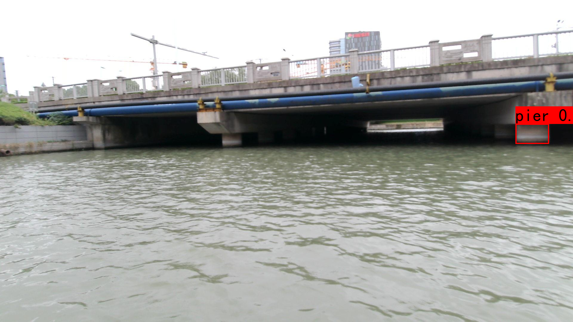
(a) NanoDet-EfficientLite

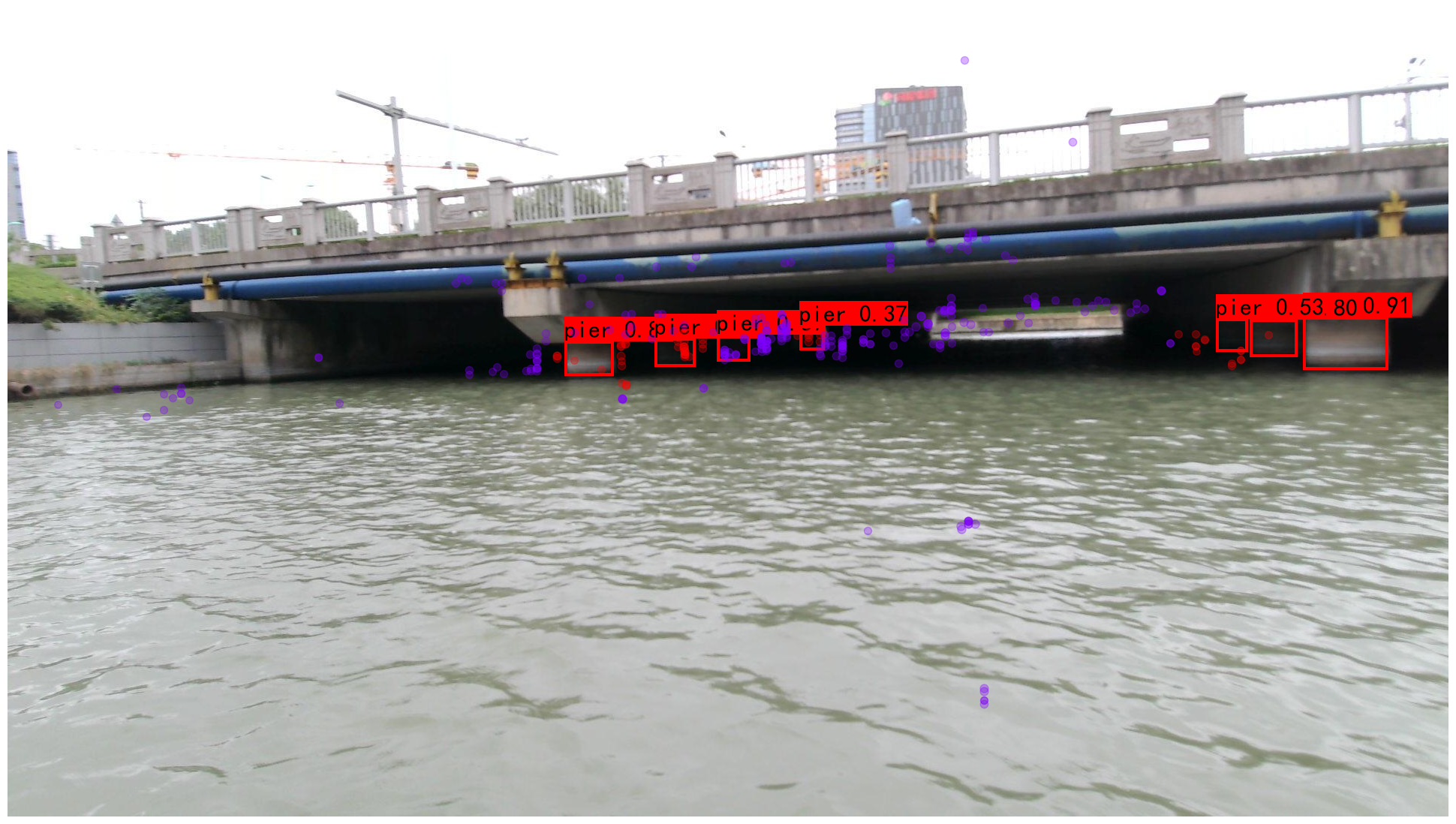
(b) Efficient-VRNet-N

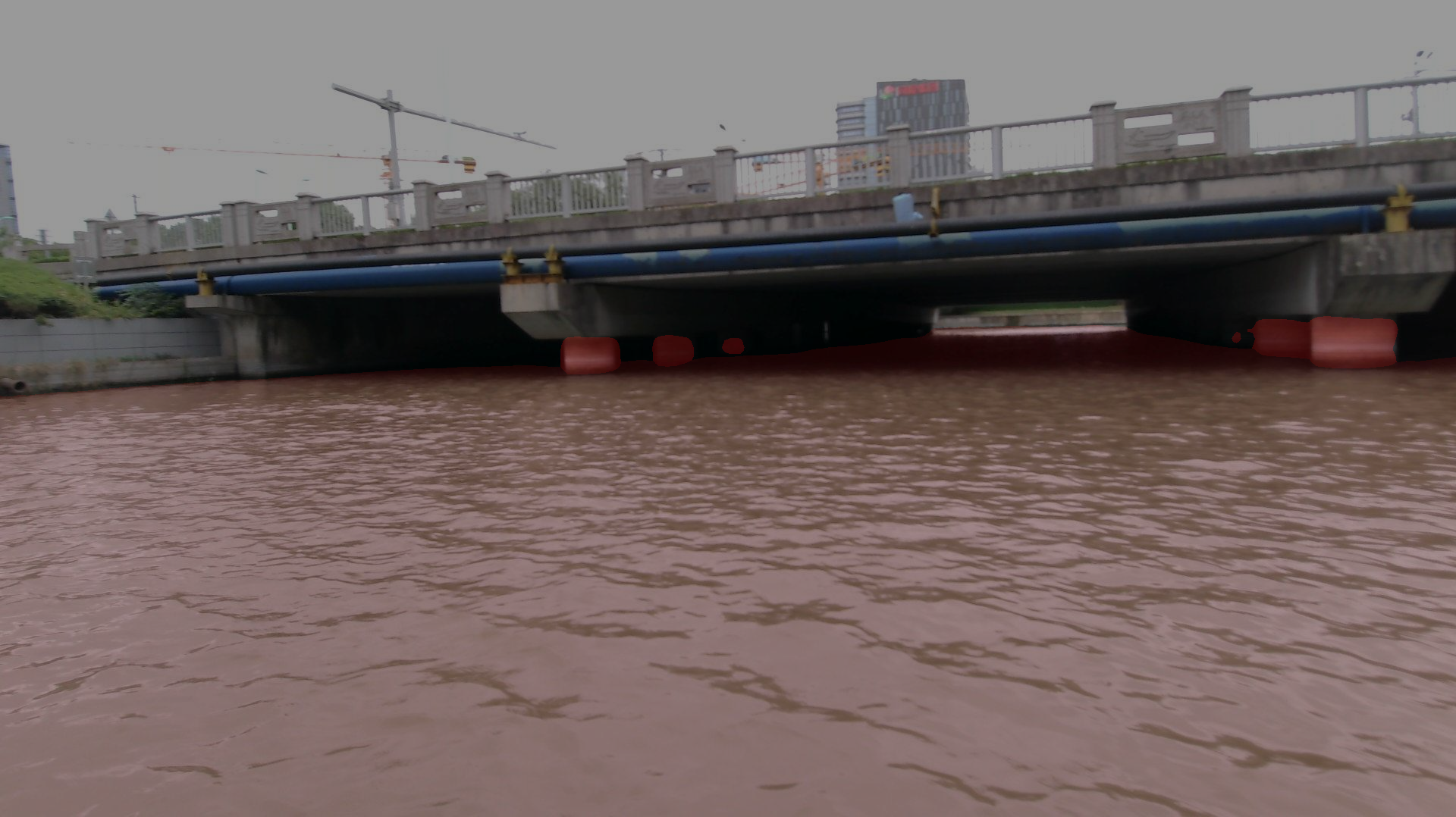
(c) PSPNet

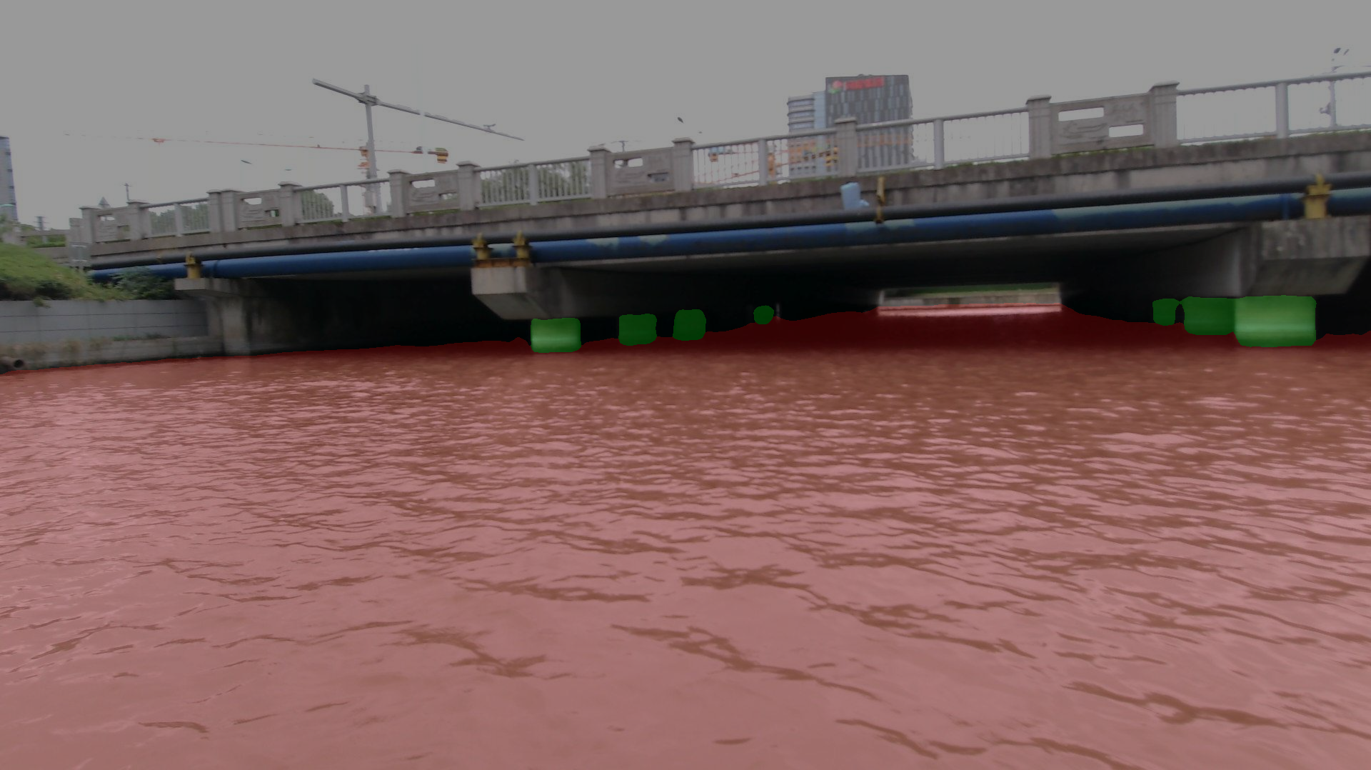
(d) Efficient-VRNet-N

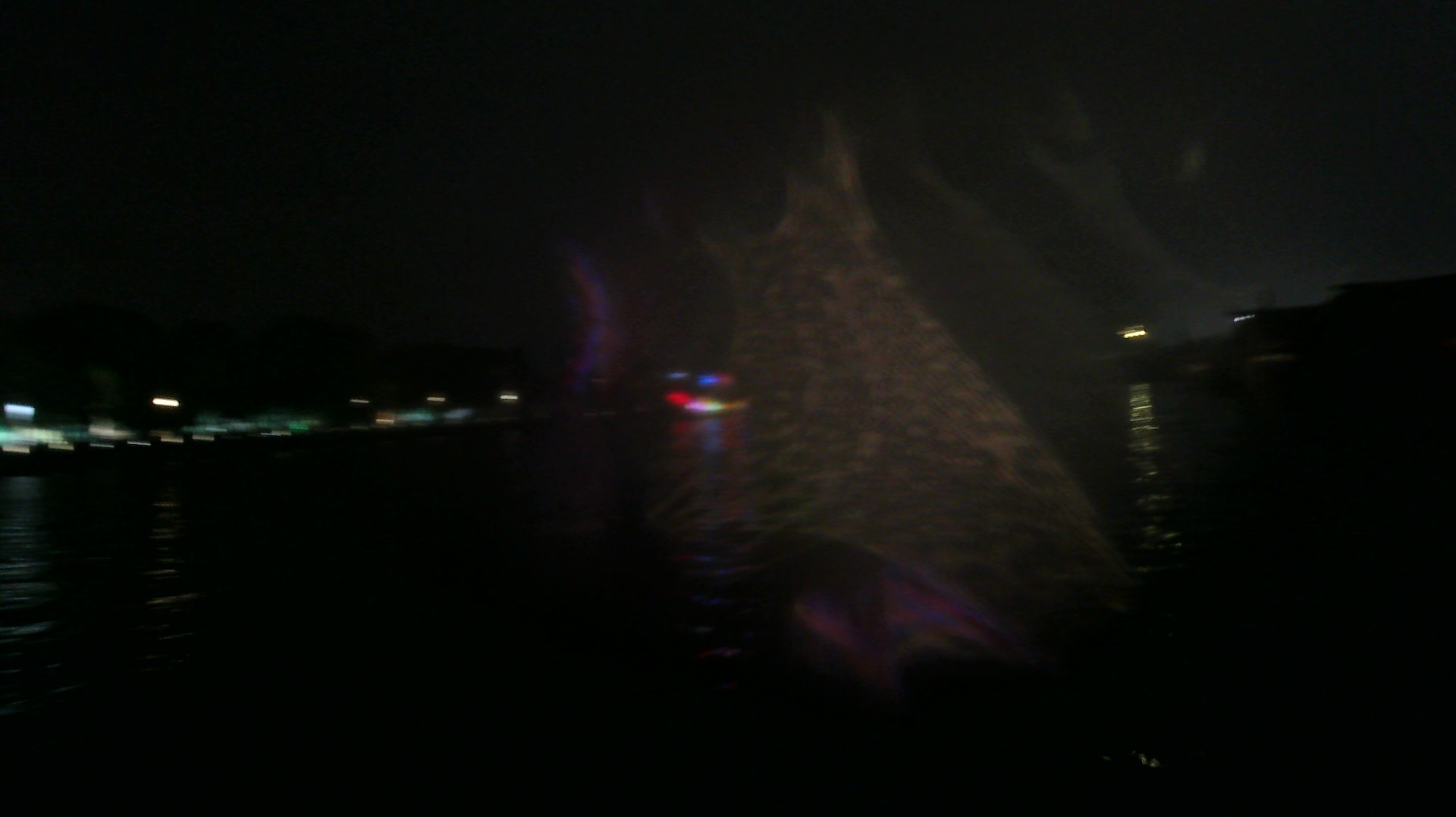
(e) YOLOX-S

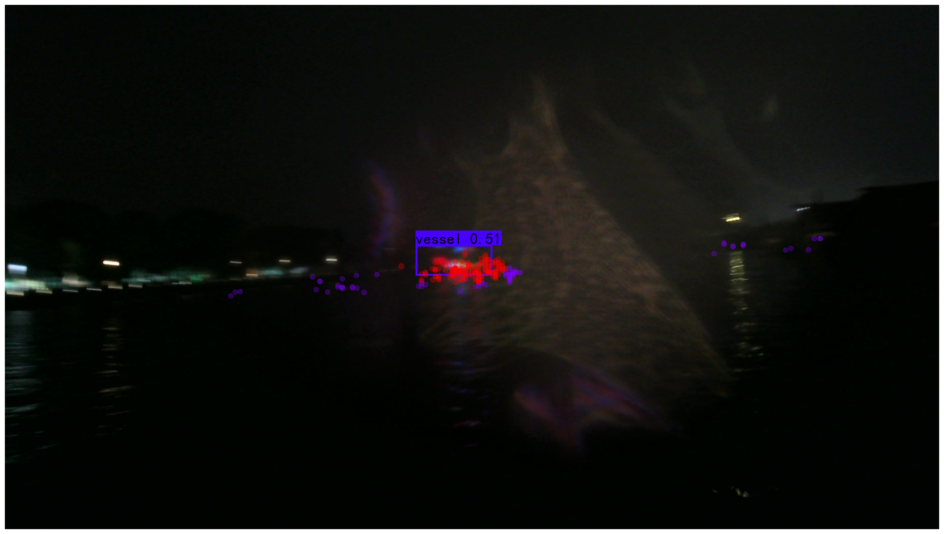
(f) Efficient-VRNet-T

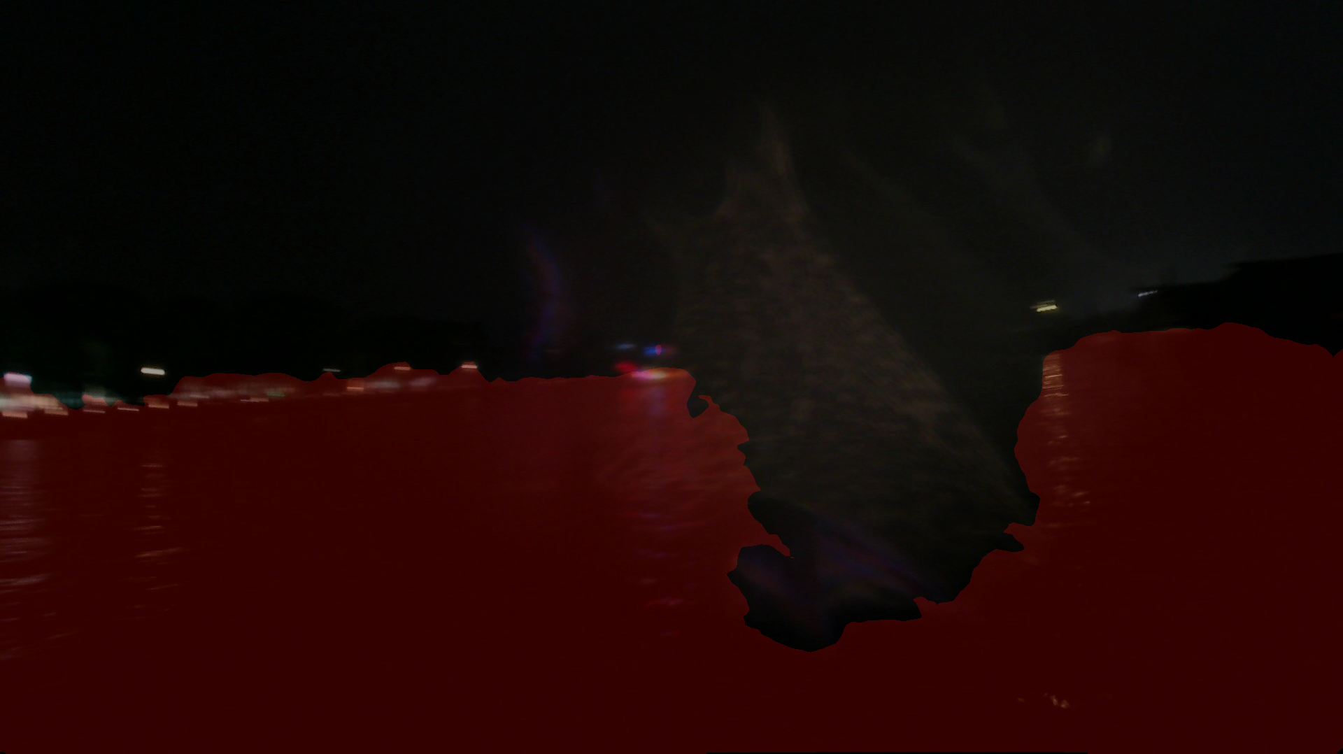
(g) DeepLabv3+ (MobileNet)

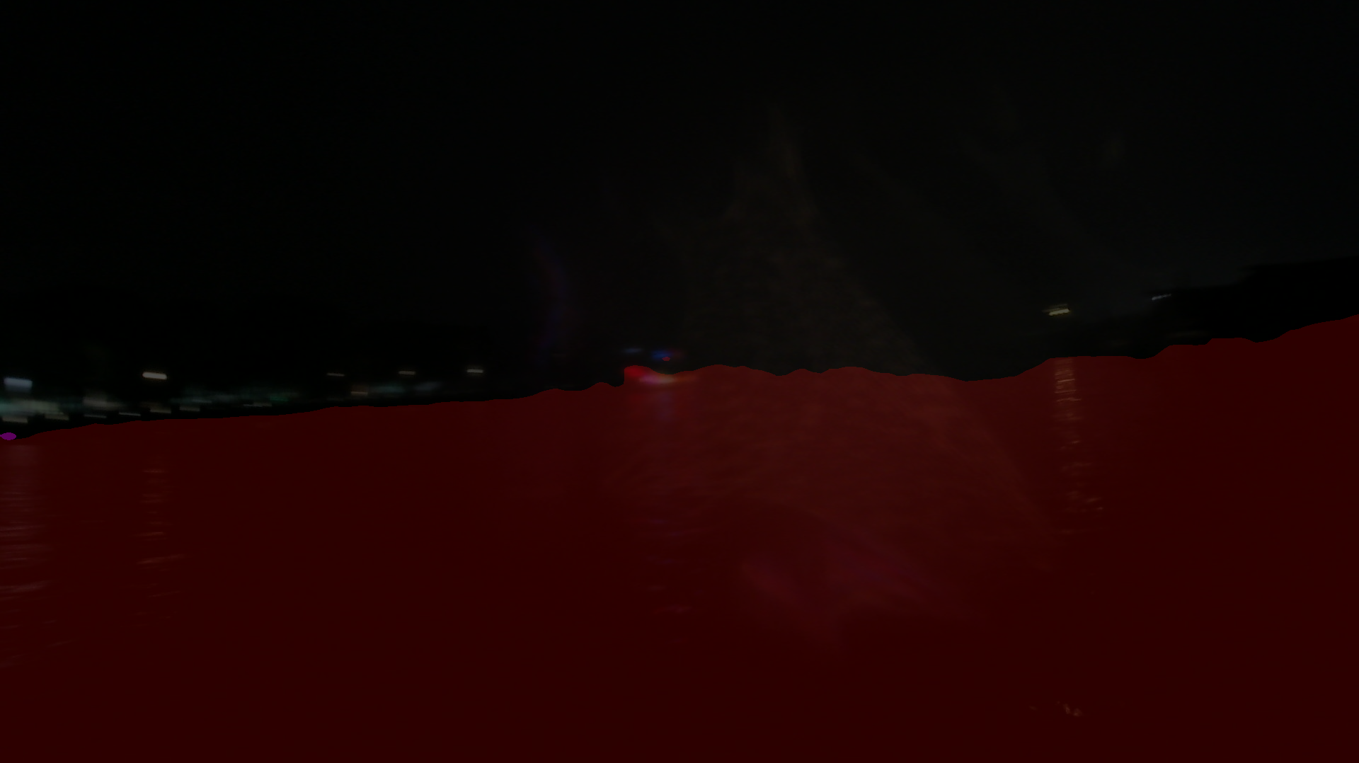
(h) Efficient-VRNet-T

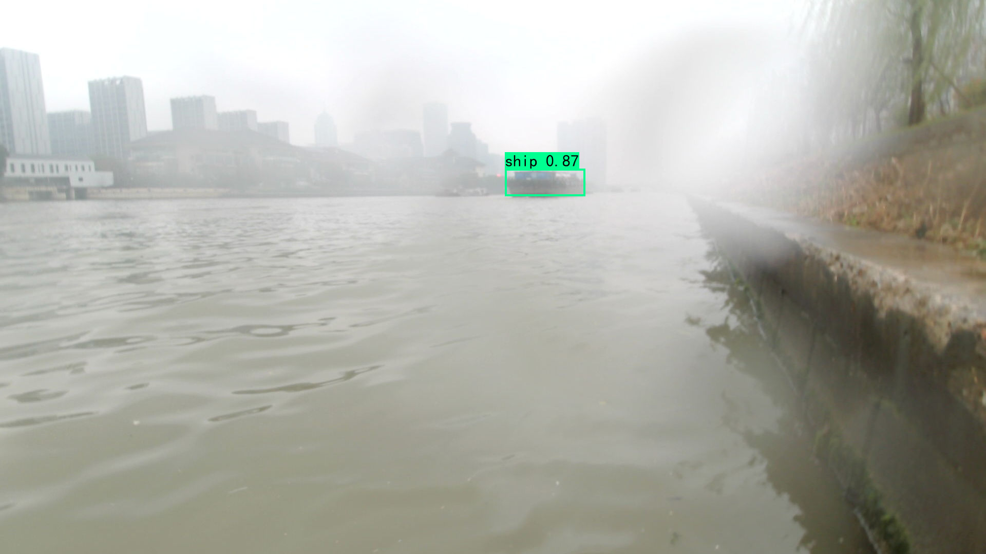
(i) YOLOv5-S6

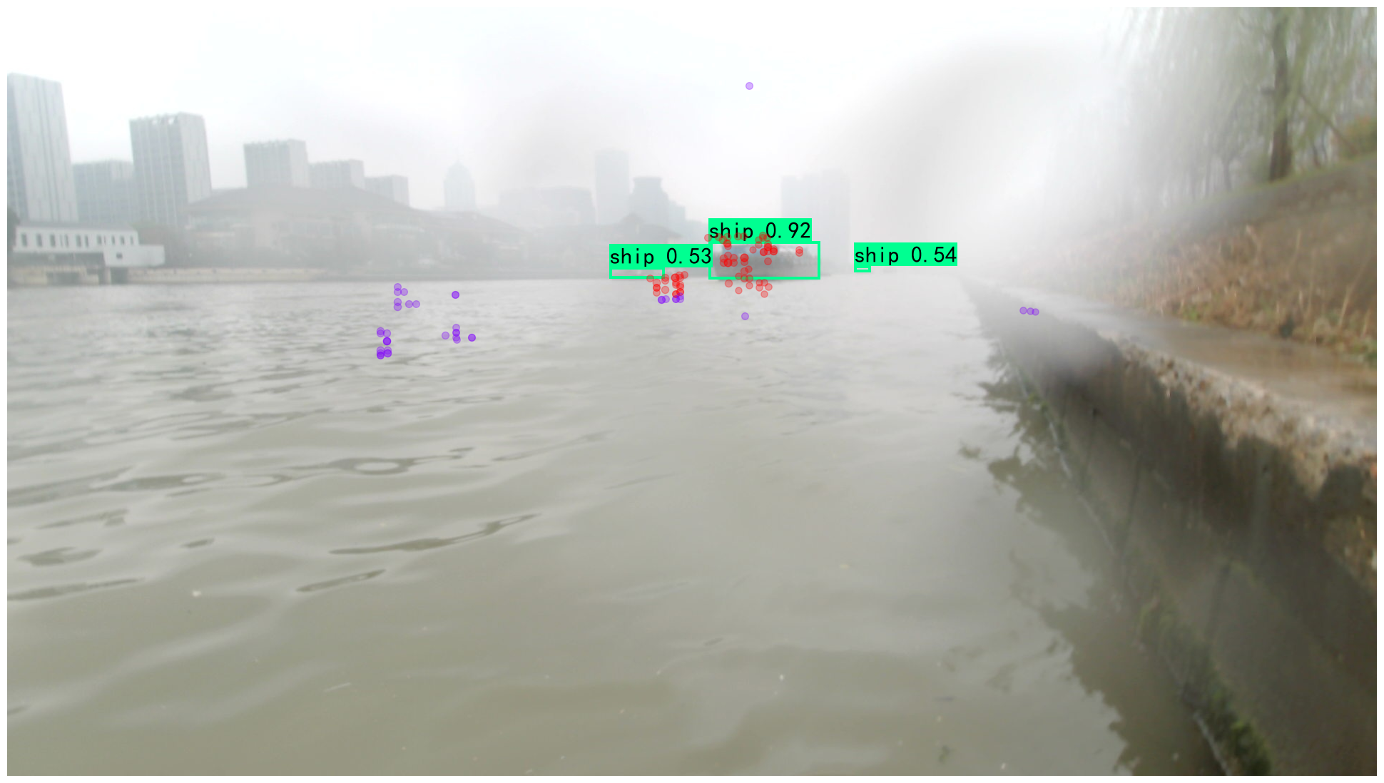
(j) Efficient-VRNet-S

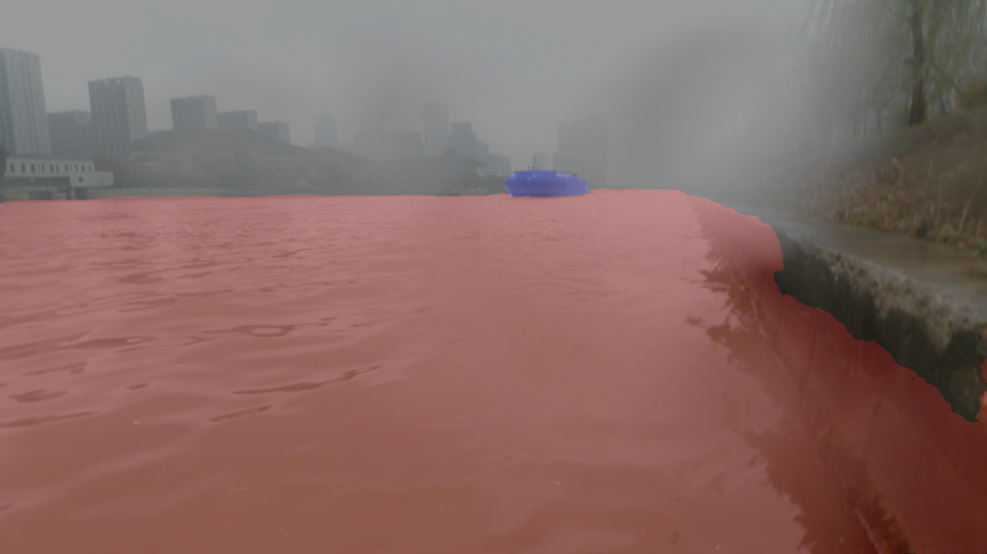
(k) HRNet-w18

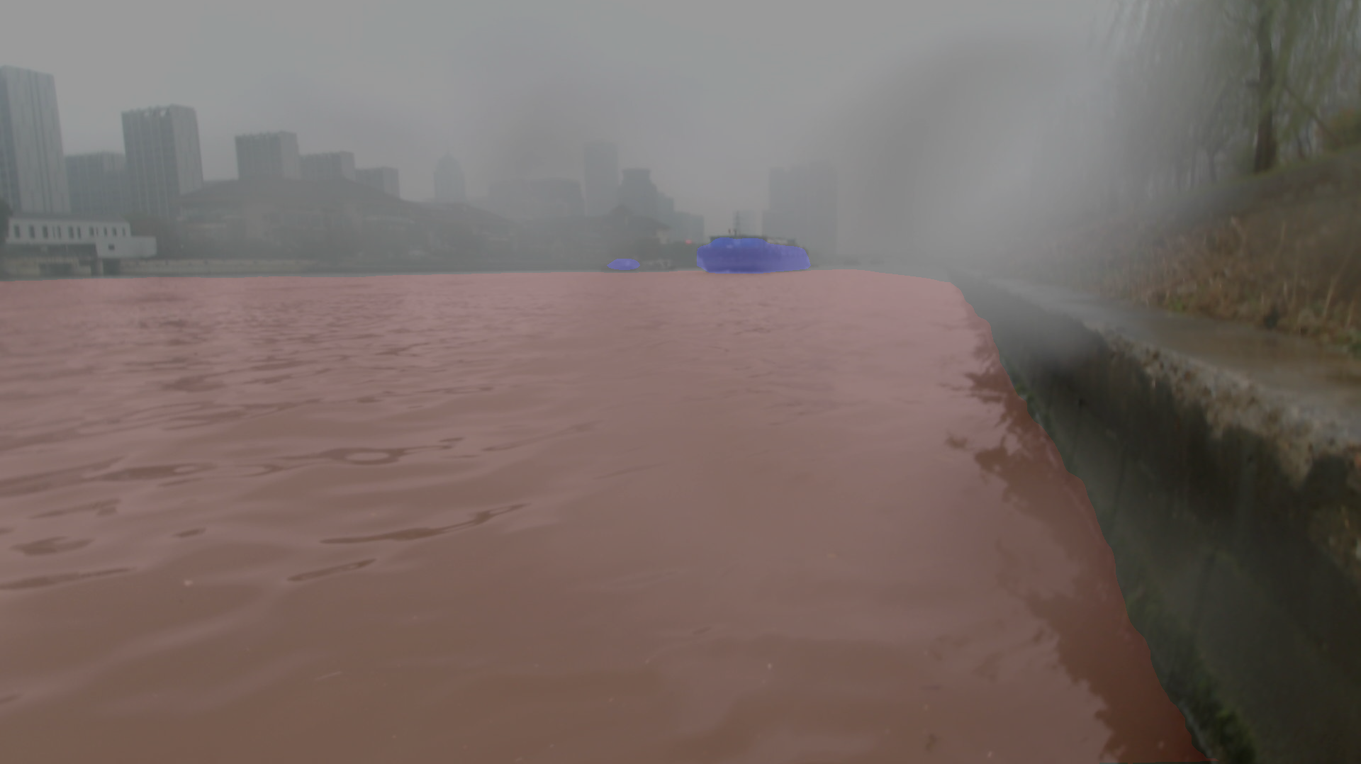
(l) Efficient-VRNet-S

Figure 12: Visualization of panoptic perception, presenting small piers in the dark environment, distant vessel at night and interfered camera, and multiple ships on a foggy day. The first column is results of pure vision models while the second column presents the detection of Efficient-VRNet family with 4D radar point clouds. The third column presents the semantic segmentation of pure vision models while the fourth column shows the segmentation of our Efficient-VRNet.

5.3 Ablation Experiments on Efficient-VRNet

Table 5: Ablation Experiments of Efficient-VRNet-N

Methods	AP50 (det)	mIoU (seg)
Efficient-VRNet-N	83.2	67.1
-RIM	-	66.9 ($\downarrow 0.2$)
-IRC	82.3 ($\downarrow 0.9$)	-
-neck fusion	83.0 ($\downarrow 0.2$)	-
-decouple detection head	82.9 ($\downarrow 0.3$)	-
multi-frame $\rightarrow$ single-frame	83.0 ($\downarrow 0.2$)	67.0 ($\downarrow 0.1$)
CoC-FPN $\rightarrow$ Conv-FPN	82.8 ($\downarrow 0.4$)	66.6 ($\downarrow 0.5$)

We conduct ablation experiments to prove the effectiveness of modules in our Efficient-VRNet. As Table 5 presents, RIM, IRC, fusion branch in the neck (neck fusion), CoC-FPN, decouple detection head and multi-frame radar data are included in ablation experiments. For object detection, IRC influences object detection the most, where AP₅₀ drops about 0.9%. Besides, after replacing CoC-FPN with the ordinary convolutional FPN, there is 0.4% drop on AP₅₀. Moreover, the fusion branch in the neck, decouple detection head and multi-frame data promote object detection performances in varying degrees. For semantic segmentation, the most practical module is CoC-FPN. We notice that mIoU drops about 0.5% after replacing CoC-FPN with the ordinary convolutional FPN. Furthermore, RIM benefits semantic segmentation to some extent. Based on the above, we find that removing CoC-FPN impacts both object detection and semantic segmentation. It implies that keeping feature structure of FPN (decoder) consistent with the backbone (encoder) is essential.

5.4 Experiments of Homoscedastic-Uncertainty-based MTL

As Table 6 presents, we adopt two kinds of multi-task training methods to train our Efficient-VRNet-N, where uncertainty weighting and manual weighting are task-joint methods while StepByStep is a task-separate method. The homoscedastic-uncertainty-based training method presents an excellent overall performance, where the detection loss is the lowest among all and the segmentation is also optimized to a satisfying interval. If training object detection individually, we find AP₅₀ is unsatisfactory, but mIoU is the highest when training semantic segmentation only. We can observe that manually selecting weights of four sub-tasks is a tough job, whose optimization performances are worse than the homoscedastic-uncertainty-based training method. However, it is much better than the task-separate method, because when we train Efficient-VRNet step by step, we find that the performance of object detection is competitive, but semantic segmentation result is terrible. It means the weights of the model learned by semantic segmentation benefit object detection, but the catastrophic forgetting of semantic segmentation parameters happens to the model during training object detection.

Table 6: Results of Multi-Task Training Methods

Methods	Weights				loss${}_{\text{det}}$	loss${}_{\text{seg}}$	AP50	mIoU
	det${}_{\text{bbox}}$	det${}_{\text{conf}}$	det${}_{\text{cls}}$	seg${}_{\text{cls}}$
Uncertainty	✓	✓	✓	✓	4.057	0.409	83.2	67.1
Weighting
Manual	0.6	0.2	0.2	0.0	6.303	-	82.5	-
Manual	0.5	0.2	0.2	0.1	4.273	0.423	83.0	66.9
Manual	0.25	0.25	0.25	0.25	5.087	0.414	82.7	66.7
Manual	0.1	0.2	0.2	0.5	6.487	0.407	82.3	67.1
Manual	0.0	0.0	0.0	1.0	-	0.398	-	67.3
StepByStep	0.6	0.2	0.2	1.0	4.189	0.502	83.0	65.1

6 Discussion

Attention modules in IRC. Although detection and segmentation tasks can share the weights of backbone, we think there are some subtle differences between two tasks. Therefore, we add shuffle attention to re-weigh feature maps in the image branch and make it adaptive to detection, because the feature maps in the image branch are mainly for segmentation. Furthermore, the attention module can effectively alleviate the negative impact of radar clutter.

Considerations of RIM. Based on the prior experiments, we notice that concatenating radar and feature maps will cause very low mIoU and f-score. It is easy to understand, because radar point cloud is a kind of local intense noise to image when concatenating it to image feature. It will compel model to weigh pixel mistakenly. Therefore, RIM can enhance the image features of corresponding positions by radar features, on the condition of not destroying image feature.

What is the meaning of fair in AFF? Fairness exists in many aspects in our Efficient-VRNet. Firstly, past works underestimated the effect of radar and only focus on detection task. We prove that radar can also improve segmentation if properly used. Secondly, past works attached more importance to image feature and did not look after feature extraction of radar features, which was unfair to radar.

7 Conclusion

We propose an exquisite panoptic perception model called Efficient-VRNet based on asymmetric fair fusion of RGB images and 4D radar point clouds, which is also the first open-source panoptic perception model. It takes both images and radar point clouds as irregular point sets and has competitive performances compared with other state-of-the-art single-task models. It also achieves better performances than other vision-based panoptic perception models. Moreover, RIM and IRC, as two asymmetric fusion modules, can behave as plug-and-play modules for any vision-radar-fusion models, because these two modules do not change the spatial and channel sizes of feature maps. Furthermore, we also subtly adapt the homoscedastic-uncertainty-based multi-task training method to panoptic perception tasks and prove its effectiveness.

Runwei_Guan.jpg Runwei Guan (Student Member, IEEE), received his M.S. degree in Data Science from University of Southampton, Southampton, United Kingdom, in 2021. He is currently a joint Ph.D. student of University of Liverpool, Xi’an Jiaotong-Liverpool University and Institute of Deep Perception Technology, Jiangsu Industrial Technology Research Institute. His research interests include visual grounding, panoptic perception based on the fusion of radar and camera, lightweight neural network, multi-task learning and statistical machine learning. He serves as the peer reviewer of IEEE TRANSACTIONS ON NEURAL NETWORKS AND LEARNING SYSTEMS, Engineering Applications of Artificial Intelligence, Journal of Supercomputing, IJCNN, etc.

yao.jpg Shanliang Yao (Student Member, IEEE), received the B.E. degree in 2016 from the School of Computer Science and Technology, Soochow University, Suzhou, China, and the M.S. degree in 2021 from the Faculty of Science and Engineering, University of Liverpool, Liverpool, U.K. He is currently working toward the Ph.D. degree with the Faculty of Science and Engineering, University of Liverpool, Liverpool, U.K. His current research is centered on multi-modal perception using deep learning approach for autonomous driving. He is also interested in robotics, autonomous vehicles and intelligent transportation systems.

xiaohuizhu.jpg Xiaohui Zhu (Member, IEEE) received his Ph.D. from the University of Liverpool, UK in 2019. He is currently an assistant professor, PhD supervisor and Programme Director with the Department of Computing, School of Advanced Technology, Xi’an Jiaotong-Liverpool University. His research interests include path planning, autonomous navigation and obstacle avoidance, and AI applications on unmanned surface vehicles.

kalok.jpg Ka Lok Man (Member, IEEE), received the Dr.Eng. degree in electronic engineering from the Politecnico di Torino, Turin, Italy, in 1998, and the Ph.D. degree in computer science from Technische Universiteit Eindhoven, Eindhoven, The Netherland, in 2006. He is currently a Professor in Computer Science and Software Engineering with Xi’an Jiaotong-Liverpool University, Suzhou, China. His research interests include formal methods and process algebras, embedded system design and testing, and photovoltaics.

yueyong.jpg Yong Yue, Fellow of Institution of Engineering and Technology (FIET), received the B.Eng. degree in mechanical engineering from Northeastern University, Shenyang, China, in 1982, and the Ph.D. degree in computer aided design from Heriot-Watt University, Edinburgh, U.K., in 1994. He worked in the industry for eight years and followed experience in academia with the University of Nottingham, Cardiff University, and the University of Bedfordshire, U.K. He is currently a Professor and Director with the Virtual Engineering Centre, Xi’an Jiaotong-Liverpool University, Suzhou, China. His current research interests include computer graphics, virtual reality, and robot navigation.

smith.jpg Jeremy Smith (Member, IEEE), received the B.Eng. (Hons.) degree in engineering science and the Ph.D. degree in electrical engineering from the University of Liverpool, Liverpool, U.K., in 1984 and 1990, respectively. Between 1984 and 1988, he was conducting research on image processing and robotic systems in the Department of Electrical Engineering and Electronics, University of Liverpool, Liverpool, U.K., where he was a Lecturer, Senior Lecturer, and Reader in the same department since 1988. Since 2006, he has been a Professor in electrical engineering with the University of Liverpool. His research interests include automated welding, robotics, vision systems, adaptive control, and embedded computer systems.

lim.jpg Eng Gee Lim (Senior Member, IEEE), received the B.Eng. (Hons.) and Ph.D. degrees in Electrical and Electronic Engineering (EEE) from Northumbria University, Newcastle, U.K., in 1998 and 2002, respectively. He worked for Andrew Ltd., Coventry, U.K., a leading communications systems company from 2002 to 2007. Since 2007, he has been with Xi’an Jiaotong–Liverpool University, Suzhou, China, where he was the Head of the EEE Department, and the University Dean of research and graduate studies. He is currently the School Dean of Advanced Technology, the Director of the AI University Research Centre, and a Professor with the Department of EEE. He has authored or coauthored over 100 refereed international journals and conference papers. His research interests are artificial intelligence (AI), robotics, AI+ health care, international standard (ISO/IEC) in robotics, antennas, RF/microwave engineering, EM measurements/simulations, energy harvesting, power/energy transfer, smart-grid communication, and wireless communication networks for smart and green cities. He is a Charted Engineer and a fellow of The Institution of Engineering and Technology (IET) and Engineers Australia. He is also a Senior Fellow of Higher Education Academy (HEA).

yueyutao.jpg Yutao Yue (Member, IEEE), was born in Qingzhou, Shandong, China, in 1982. He received the B.S. degree in applied physics from the University of Science and Technology of China, in 2004, and the M.S. and Ph.D. degrees in computational physics from Purdue University, USA, in 2006 and 2010, respectively. From 2011 to 2017, he worked as a Senior Scientist with the Shenzhen Kuang-Chi Institute of Advanced Technology and a Team Leader of the Guangdong “Zhujiang Plan” 3rd Introduced Innovation Scientific Research Team. From 2017 to 2018, he was a Research Associate Professor with the Southern University of Science and Technology, China. Since 2018, he has been the Founder and the Director of the Institute of Deep Perception Technology, JITRI, Jiangsu, China. Since 2020, he has been working as an Honorary Recognized Ph.D. Advisor of the University of Liverpool, U.K., and Xi’an Jiaotong-Liverpool University, China. He is the co-inventor of over 300 granted patents of China, USA, and Europe. He is also the author of over 20 journals and conference papers. His research interests include computational modeling, radar vision fusion, perception and cognition cooperation, artificial intelligence theory, and electromagnetic field modulation. Dr. Yue was a recipient of the WuWen Jun Artificial Intelligence Science and Technology Award in 2020.

References

- Achanta et al. [2012] Achanta, R., Shaji, A., Smith, K., Lucchi, A., Fua, P., Süsstrunk, S., 2012. Slic superpixels compared to state-of-the-art superpixel methods. IEEE transactions on pattern analysis and machine intelligence 34, 2274–2282.
- Bovcon et al. [2019] Bovcon, B., Muhovič, J., Perš, J., Kristan, M., 2019. The mastr1325 dataset for training deep usv obstacle detection models, in: 2019 IEEE/RSJ International Conference on Intelligent Robots and Systems (IROS), IEEE. pp. 3431–3438.
- Broedermann et al. [2022] Broedermann, T., Sakaridis, C., Dai, D., Van Gool, L., 2022. Hrfuser: A multi-resolution sensor fusion architecture for 2d object detection. arXiv preprint arXiv:2206.15157 .
- Buslaev et al. [2020] Buslaev, A., Iglovikov, V.I., Khvedchenya, E., Parinov, A., Druzhinin, M., Kalinin, A.A., 2020. Albumentations: Fast and flexible image augmentations. Information 11. URL: https://www.mdpi.com/2078-2489/11/2/125, doi:10.3390/info11020125.
- Chen et al. [2018a] Chen, L.C., Zhu, Y., Papandreou, G., Schroff, F., Adam, H., 2018a. Encoder-decoder with atrous separable convolution for semantic image segmentation, in: Proceedings of the European conference on computer vision (ECCV), pp. 801–818.
- Chen et al. [2018b] Chen, Z., Badrinarayanan, V., Lee, C.Y., Rabinovich, A., 2018b. Gradnorm: Gradient normalization for adaptive loss balancing in deep multitask networks, in: International conference on machine learning, PMLR. pp. 794–803.
- Cheng et al. [2021a] Cheng, Y., Jiang, M., Zhu, J., Liu, Y., 2021a. Are we ready for unmanned surface vehicles in inland waterways? the usvinland multisensor dataset and benchmark. IEEE Robotics and Automation Letters 6, 3964–3970.
- Cheng et al. [2021b] Cheng, Y., Xu, H., Liu, Y., 2021b. Robust small object detection on the water surface through fusion of camera and millimeter wave radar, in: Proceedings of the IEEE/CVF International Conference on Computer Vision, pp. 15263–15272.
- Cheng et al. [2021c] Cheng, Y., Zhu, J., Jiang, M., Fu, J., Pang, C., Wang, P., Sankaran, K., Onabola, O., Liu, Y., Liu, D., et al., 2021c. Flow: A dataset and benchmark for floating waste detection in inland waters, in: Proceedings of the IEEE/CVF International Conference on Computer Vision, pp. 10953–10962.
- Dosovitskiy et al. [2020] Dosovitskiy, A., Beyer, L., Kolesnikov, A., Weissenborn, D., Zhai, X., Unterthiner, T., Dehghani, M., Minderer, M., Heigold, G., Gelly, S., et al., 2020. An image is worth 16x16 words: Transformers for image recognition at scale, in: International Conference on Learning Representations.
- Farahnakian et al. [2018] Farahnakian, F., Haghbayan, M.H., Poikonen, J., Laurinen, M., Nevalainen, P., Heikkonen, J., 2018. Object detection based on multi-sensor proposal fusion in maritime environment, in: 2018 17th IEEE International Conference on Machine Learning and Applications (ICMLA), IEEE. pp. 971–976.
- Ge et al. [2021] Ge, Z., Liu, S., Wang, F., Li, Z., Sun, J., 2021. Yolox: Exceeding yolo series in 2021. arXiv preprint arXiv:2107.08430 .
- Haghbayan et al. [2018] Haghbayan, M.H., Farahnakian, F., Poikonen, J., Laurinen, M., Nevalainen, P., Plosila, J., Heikkonen, J., 2018. An efficient multi-sensor fusion approach for object detection in maritime environments, in: 2018 21st International Conference on Intelligent Transportation Systems (ITSC), IEEE. pp. 2163–2170.
- Han et al. [2022] Han, C., Zhao, Q., Zhang, S., Chen, Y., Zhang, Z., Yuan, J., 2022. Yolopv2: Better, faster, stronger for panoptic driving perception. arXiv preprint arXiv:2208.11434 .
- Jocher [2021] Jocher, G., 2021. Yolov5.
- John and Mita [2019] John, V., Mita, S., 2019. Rvnet: Deep sensor fusion of monocular camera and radar for image-based obstacle detection in challenging environments, in: Pacific-Rim Symposium on Image and Video Technology, Springer. pp. 351–364.
- John et al. [2019] John, V., Nithilan, M.K., Mita, S., Tehrani, H., Sudheesh, R.S., Lalu, P.P., 2019. So-net: Joint semantic segmentation and obstacle detection using deep fusion of monocular camera and radar, Springer-Verlag. p. 138–148. URL: https://doi.org/10.1007/978-3-030-39770-8_11, doi:10.1007/978-3-030-39770-8_11.
- Kendall et al. [2018] Kendall, A., Gal, Y., Cipolla, R., 2018. Multi-task learning using uncertainty to weigh losses for scene geometry and semantics, in: Proceedings of the IEEE conference on computer vision and pattern recognition, pp. 7482–7491.
- Kim et al. [2021] Kim, K., Kim, J., Kim, J., 2021. Robust data association for multi-object detection in maritime environments using camera and radar measurements. IEEE Robotics and Automation Letters 6, 5865–5872.
- Kumar et al. [2021] Kumar, V.R., Yogamani, S., Rashed, H., Sitsu, G., Witt, C., Leang, I., Milz, S., Mäder, P., 2021. Omnidet: Surround view cameras based multi-task visual perception network for autonomous driving. IEEE Robotics and Automation Letters 6, 2830–2837.
- Li and Xie [2020] Li, L.q., Xie, Y.l., 2020. A feature pyramid fusion detection algorithm based on radar and camera sensor, in: 2020 15th IEEE International Conference on Signal Processing (ICSP), IEEE. pp. 366–370.
- Lin et al. [2021] Lin, F., Hou, T., Jin, Q., You, A., 2021. Improved yolo based detection algorithm for floating debris in waterway. Entropy 23, 1111.
- Lin et al. [2014] Lin, T.Y., Maire, M., Belongie, S., Hays, J., Perona, P., Ramanan, D., Dollár, P., Zitnick, C.L., 2014. Microsoft coco: Common objects in context, in: Computer Vision–ECCV 2014: 13th European Conference, Zurich, Switzerland, September 6-12, 2014, Proceedings, Part V 13, Springer. pp. 740–755.
- Liu et al. [2019] Liu, S., Johns, E., Davison, A.J., 2019. End-to-end multi-task learning with attention, in: Proceedings of the IEEE/CVF conference on computer vision and pattern recognition, pp. 1871–1880.
- Lyridis [2021] Lyridis, D.V., 2021. An improved ant colony optimization algorithm for unmanned surface vehicle local path planning with multi-modality constraints. Ocean Engineering 241, 109890.
- Ma et al. [2023] Ma, X., Zhou, Y., Wang, H., Qin, C., Sun, B., Liu, C., Fu, Y., 2023. Image as set of points, in: International Conference on Learning Representations. URL: https://openreview.net/forum?id=awnvqZja69.
- Madeo et al. [2020] Madeo, D., Pozzebon, A., Mocenni, C., Bertoni, D., 2020. A low-cost unmanned surface vehicle for pervasive water quality monitoring. IEEE Transactions on Instrumentation and Measurement 69, 1433–1444.
- Maharjan et al. [2022] Maharjan, N., Miyazaki, H., Pati, B.M., Dailey, M.N., Shrestha, S., Nakamura, T., 2022. Detection of river plastic using uav sensor data and deep learning. Remote Sensing 14, 3049.
- Nobis et al. [2019] Nobis, F., Geisslinger, M., Weber, M., Betz, J., Lienkamp, M., 2019. A deep learning-based radar and camera sensor fusion architecture for object detection, in: 2019 Sensor Data Fusion: Trends, Solutions, Applications (SDF), IEEE. pp. 1–7.
- RangiLyu [2021] RangiLyu, 2021. Nanodet-plus: Super fast and high accuracy lightweight anchor-free object detection model. https://github.com/RangiLyu/nanodet.
- Sener and Koltun [2018] Sener, O., Koltun, V., 2018. Multi-task learning as multi-objective optimization. Advances in neural information processing systems 31.
- Song et al. [2022] Song, Y., Xie, Z., Wang, X., Zou, Y., 2022. Ms-yolo: Object detection based on yolov5 optimized fusion millimeter-wave radar and machine vision. IEEE Sensors Journal 22, 15435–15447.
- Sorial et al. [2019] Sorial, M., Mouawad, I., Simetti, E., Odone, F., Casalino, G., 2019. Towards a real time obstacle detection system for unmanned surface vehicles, in: OCEANS 2019 MTS/IEEE SEATTLE, pp. 1–8. doi:10.23919/OCEANS40490.2019.8962685.
- Stäcker et al. [2022] Stäcker, L., Heidenreich, P., Rambach, J., Stricker, D., 2022. Fusion point pruning for optimized 2d object detection with radar-camera fusion, in: Proceedings of the IEEE/CVF Winter Conference on Applications of Computer Vision, pp. 3087–3094.
- Vu et al. [2022] Vu, D., Ngo, B., Phan, H., 2022. Hybridnets: End-to-end perception network. arXiv preprint arXiv:2203.09035 .
- Wang et al. [2022] Wang, C.Y., Bochkovskiy, A., Liao, H.Y.M., 2022. Yolov7: Trainable bag-of-freebies sets new state-of-the-art for real-time object detectors. arXiv preprint arXiv:2207.02696 .
- Wang et al. [2020a] Wang, J., Sun, K., Cheng, T., Jiang, B., Deng, C., Zhao, Y., Liu, D., Mu, Y., Tan, M., Wang, X., et al., 2020a. Deep high-resolution representation learning for visual recognition. IEEE transactions on pattern analysis and machine intelligence 43, 3349–3364.
- Wang et al. [2020b] Wang, Q., Wu, B., Zhu, P., Li, P., Zuo, W., Hu, Q., 2020b. Eca-net: Efficient channel attention for deep convolutional neural networks, in: Proceedings of the IEEE/CVF conference on computer vision and pattern recognition, pp. 11534–11542.
- Wu et al. [2022] Wu, D., Liao, M.W., Zhang, W.T., Wang, X.G., Bai, X., Cheng, W.Q., Liu, W.Y., 2022. Yolop: You only look once for panoptic driving perception. Machine Intelligence Research , 1–13.
- Xie et al. [2021] Xie, E., Wang, W., Yu, Z., Anandkumar, A., Alvarez, J.M., Luo, P., 2021. Segformer: Simple and efficient design for semantic segmentation with transformers. Advances in Neural Information Processing Systems 34, 12077–12090.
- Xue et al. [2019] Xue, Z., Liu, J., Wu, Z., Du, S., Kong, S., Yu, J., 2019. Development and path planning of a novel unmanned surface vehicle system and its application to exploitation of qarhan salt lake. Science China Information Sciences 62, 1–3.
- Yang et al. [2020] Yang, T., Jiang, Z., Sun, R., Cheng, N., Feng, H., 2020. Maritime search and rescue based on group mobile computing for unmanned aerial vehicles and unmanned surface vehicles. IEEE transactions on industrial informatics 16, 7700–7708.
- Yang et al. [2022] Yang, X., Zhao, J., Zhao, L., Zhang, H., Li, L., Ji, Z., Ganchev, I., 2022. Detection of river floating garbage based on improved yolov5. Mathematics 10, 4366.
- Zailan et al. [2022] Zailan, N.A., Azizan, M.M., Hasikin, K., Khairuddin, A.S.M., Khairuddin, U., 2022. An automated solid waste detection using the optimized yolo model for riverine management. Frontiers in Public Health 10.
- Zhang et al. [2021a] Zhang, L., Wei, Y., Wang, H., Shao, Y., Shen, J., 2021a. Real-time detection of river surface floating object based on improved refinedet. IEEE Access 9, 81147–81160.
- Zhang and Yang [2021] Zhang, Q.L., Yang, Y.B., 2021. Sa-net: Shuffle attention for deep convolutional neural networks, in: ICASSP 2021-2021 IEEE International Conference on Acoustics, Speech and Signal Processing (ICASSP), IEEE. pp. 2235–2239.
- Zhang et al. [2021b] Zhang, W., Jiang, F., Yang, C.F., Wang, Z.P., Zhao, T.J., 2021b. Research on unmanned surface vehicles environment perception based on the fusion of vision and lidar. IEEE Access 9, 63107–63121.
- Zhang et al. [2021c] Zhang, Z., Lu, X., Cao, G., Yang, Y., Jiao, L., Liu, F., 2021c. Vit-yolo: Transformer-based yolo for object detection, in: Proceedings of the IEEE/CVF international conference on computer vision, pp. 2799–2808.
- Zhao et al. [2017] Zhao, H., Shi, J., Qi, X., Wang, X., Jia, J., 2017. Pyramid scene parsing network, in: Proceedings of the IEEE conference on computer vision and pattern recognition, pp. 2881–2890.
- Zhu et al. [2019] Zhu, X., Yue, Y., Wong, P.W., Zhang, Y., Ding, H., 2019. Designing an optimized water quality monitoring network with reserved monitoring locations. Water 11, 713.