Minimalist Traffic Prediction: Linear Layer Is All You Need

Abstract

Traffic prediction is essential for the progression of Intelligent Transportation Systems (ITS) and the vision of smart cities. While Spatial-Temporal Graph Neural Networks (STGNNs) have shown promise in this domain by leveraging Graph Neural Networks (GNNs) integrated with either RNNs or Transformers, they present challenges such as computational complexity, gradient issues, and resource-intensiveness. This paper addresses these challenges, advocating for three main solutions: a node-embedding approach, time series decomposition, and periodicity learning. We introduce STLinear, a minimalist model architecture designed for optimized efficiency and performance. Unlike traditional STGNNs, STLinear operates fully locally, avoiding inter-node data exchanges, and relies exclusively on linear layers, drastically cutting computational demands. Our empirical studies on real-world datasets confirm STLinear’s prowess, matching or exceeding the accuracy of leading STGNNs, but with significantly reduced complexity and computation overhead (more than 95% reduction in MACs per epoch compared to state-of-the-art STGNN baseline published in 2023). In summary, STLinear emerges as a potent, efficient alternative to conventional STGNNs, with profound implications for the future of ITS and smart city initiatives.

Introduction

Traffic prediction is fundamental to Intelligent Transportation Systems (ITS), which aim to bolster the efficiency and safety of urban traffic management. By leveraging historical data, traffic flow prediction strives to forecast future traffic conditions. Precise predictions can drive the growth of smart cities by curbing traffic congestion, cutting fuel consumption, reducing greenhouse gas emissions, and minimizing road accidents. A key characteristic of traffic data is the strong correlation among time series due to the interconnectedness of the road network. For precise traffic prediction, numerous state-of-the-art approaches (Yu, Yin, and Zhu 2018; Wu et al. 2019; Huang et al. 2020; Zheng et al. 2020; Li and Zhu 2021; Choi et al. 2022; Jiang et al. 2023) employ Spatial-Temporal Graph Neural Networks (STGNNs).

Spatial-Temporal Graph Neural Networks (STGNNs) are tailored for processing spatial-temporal data, merging two essential components: a spatial module and a temporal module. The spatial module harnesses the power of Graph Neural Networks (GNNs) to model spatial information, capturing intricate relationships between entities. Conversely, for temporal information, both Recurrent Neural Networks (RNNs) (Connor, Atlas, and Martin 1992; Li et al. 2018; Bai et al. 2020) and Transformers (Vaswani et al. 2017; Jiang et al. 2023; Guo et al. 2023) have been utilized in STGNN research. This union of either RNNs or Transformers with GNNs supercharges STGNNs for tasks like traffic prediction. Nonetheless, STGNNs present their own challenges:

• Complexity of GNNs: While GNNs are undoubtedly effective, they aren’t optimized in terms of resource utilization. Their integration into the STGNN framework amplifies both the computational and structural complexities. This can lead to increased resource demands and extended training periods. As an illustrative example, consider the adaptive graph convolution network (AGCN), a key advancement within STGNNs. The inference time complexity of a single AGCN layer is denoted by $\mathcal{O}(N^{2})$, where $N$ represents the number of nodes (Duan et al. 2023).

• RNNs and Gradient Issues: While RNNs excel at modeling short-term dependencies, they are susceptible to gradient explosion and vanishing, especially with extended data sequences. This not only affects prediction accuracy but also complicates training, often requiring specialized techniques or interventions.

• Resource Intensive Transformers: Although Transformers excel at handling long-term dependencies due to their multi-head self-attention mechanism, they can be resource-intensive, especially on large datasets, making them less suitable for certain real-time or resource-restricted applications.

In summary, despite the successes of STGNN-based techniques, they grapple with challenges like growing complexity and marginal improvements, especially for long-term traffic prediction across many nodes. This raises the question: Is it possible to develop a model as proficient as STGNNs but more efficient in both training and inference? Given recent advancements in spatial-temporal data processing research, we have pinpointed potential solutions for STGNNs’ efficiency constraints:

1. Recent findings (Duan et al. 2023) suggest that temporal dependency is paramount for inference in many spatial-temporal tasks. It suggests that current STGNN structures might overemphasize spatial dependency modeling, leading to increased overhead and reduced scalability. Nonetheless, the inherent spatial attributes of individual nodes are vital (Bai et al. 2020), particularly during cooperative training processes. We advocate for a node-embedding approach, analogous to the soft weight sharing in multi-task learning, enabling parameter extraction from a unified weight pool.

2. The often low information density and abundant noise in traffic data highlight the need to recognize time-dependencies across varied scales. Recent studies (Zeng et al. 2023; Li et al. 2023; Ekambaram et al. 2023) propose multi-scale information abstraction as the chief method for spatial-temporal inference. They indicate that basic linear models combined with decomposition might rival or even surpass Transformers. In response, we endorse time series decomposition.

3. Traffic systems usually reflect the periodicity of human society. Many works have shown that considering periodicity is beneficial for traffic prediction (Zhou et al. 2021; Jiang et al. 2023). Recognizing the crucial role of periodic information, we present periodicity learning, an innovative mechanism to encode and smoothly integrate periodicity data into our processes.

Culminating our efforts, we propose STLinear, a minimalist design of model architecture providing state-of-the-art performance and efficiency. STLinear is fully localized, meaning it requires no inter-node data exchange during training and inference. This not only cuts down the model’s computational overhead but also facilitates its deployment on systems with communication constraints. Additionally, STLinear operates on pure linear layers, drastically reducing computational resource needs and simplifying both training and inference. The architecture is depicted in Figure. 1, with comprehensive explanations in section Method.

Our empirical assessments, carried out on four publicly available real-world datasets, demonstrate that STLinear consistently matches or even outperforms leading STGNNs in traffic prediction tasks in inference accuracy, all with significantly reduced computing overhead. For instance, when compared against SSTBAN (Guo et al. 2023), a benchmark state-of-the-art method, STLinear records a remarkable reduction in MACs per epoch during inference, ranging from 95.50% to 99.81%. During training, this efficiency becomes even more evident: STLinear exhibits a reduction in MACs per epoch between 99.10% and 99.96% and a decrease in memory usage that varies between 15.99% and 95.20%.

Related Work

Our work majorly relates to two research fields: (i) traffic prediction using STGNNs, and (ii) long time series forecasting (LTSF) with linear models.

STGNNs for Traffic Prediction

Traffic forecasting is crucial within ITS and has been a subject of study for many years. Historically, techniques like ARIMA (Makridakis and Hibon 1997) and VAR (Zivot and Wang 2006) centered on temporal dependencies for individual nodes or a small group of nodes. However, these approaches struggled with real-world traffic data that exhibited both temporal and spatial dynamics. The advent of deep learning brought to the fore the STGNNs, which have become indispensable in this domain. Their strength lies in unveiling hidden patterns of spatially irregular signals over time. Typically, these models combine graph convolutional networks (GCNs) with sequential models (e.g., RNNs, TCN, Transformer). Below, we detail the design components of prevalent STGNN-based traffic prediction methods.

Spatial Dependency Modeling

A central challenge for STGNN techniques is accurately modeling the intricate spatial dependencies between nodes, represented by the adjacency matrix. While GCNs (Yu, Yin, and Zhu 2018; Guo et al. 2019; Pan et al. 2019) are a popular choice for spatial dependency modeling, they often rely on a predetermined graph structure which might not fully encapsulate spatial dependencies (Bai et al. 2020). Graph WaveNet (Wu et al. 2019) proposed an adaptive graph convolutional (AGCN) layer that learns an adaptive adjacency matrix, bypassing the need for a preset graph. AGCRN (Bai et al. 2020) went a step further, positing that adaptive graphs alone might not be enough. This method enriches AGCN with a node adaptive parameter learning (NAPL) module, which discerns node-specific patterns using node embedding. Inspired by NAPL, we endorse a node-embedding method, akin to the soft weight sharing in multi-task learning. This allows for parameter extraction from a singular weight repository. It’s worth noting that AGCRN and its derivatives (Choi et al. 2022; Chen et al. 2022) might overemphasize spatial dependency modeling, leading to elevated overhead and diminished scalability. Distinctly, STLinear emphasizes spatial characteristics rather than sheer spatial dependencies.

Temporal Dependency Modeling

Being a unique kind of time series, STGNNs must also grapple with capturing temporal dependencies. Based on the methodologies employed to tackle time dependencies, STGNNs can be categorized into RNN-based, CNN-based, and Transformer-based models (Li et al. 2018; Bai et al. 2020; Chen, Segovia-Dominguez, and Gel 2021; Chen et al. 2022). Graph Wavenet, STSGCN, and ASTGCN stand out as CNN-based methods, whereas GMAN (Zheng et al. 2020), PDFormer (Jiang et al. 2023), and SSTBAN (Guo et al. 2023) are prominent Transformer-based techniques. Recent literature underscores the benefits of incorporating historical periodicity information for temporal dependency modeling. The straightforward approach involves injecting learnable daily and weekly periodicity embeddings into the input sequence. Contrary to this approach, STLinear incorporates the periodicity embeddings of only the initial and terminal data points in the historical dataset, optimizing for efficiency.

LTSF with linear models

Linear models have witnessed a resurgence in the LTSF domain (Shao et al. 2022; Zeng et al. 2023). For instance, LightTS leverages linear models alongside two nuanced downsampling strategies to enhance forecasting (Zhang et al. 2022). After deconstructing the time series into trend and remainder components, DLinear applies a simple linear model, even outshining Transformer-based state-of-the-art solutions (Zeng et al. 2023). TSMixer, designed around multi-layer perceptron (MLP) modules, targets multivariate long time series forecasting, presenting an efficient alternative to Transformers (Ekambaram et al. 2023). Yet, these models falter with traffic data’s unique characteristics. In contrast, STLinear adeptly incorporates periodicity and spatial attributes.

Efficient Traffic Prediction with STLinear

This section introduces STLinear, a novel method for traffic prediction that emphasizes efficiency in both training and inference stages. Refer to Figure 1 for an overview of our architecture.

Notation and Problem Definition

Adhering the conventions in STGNNs-enabled traffic forecasting (Wu et al. 2019; Bai et al. 2020; Chen et al. 2022), traffic data is denoted as $\mathcal{X}\in\mathbb{R}^{N\times T\times C}$, where $N$ stands for the number of nodes, $T$ the number of time-steps, and $C$ the number of features. A significant portion of traffic data, especially those explored in this paper, are univariate, meaning $C=1$. Thus, for simplicity, we employ $\mathcal{X}\in\mathbb{R}^{N\times T}$ without any loss of generality.

$\mathcal{X}$ can be depicted as $\{\mathbf{x}_{:,1},\mathbf{x}_{:,2},\ldots,\mathbf{x}_{:,T}\}$ with $\mathbf{x}_{:,t}\in\mathbb{R}^{N}$ being a “snap shot” of all nodes’ feature at time $t$, or as $\{\mathbf{x}_{1,:},\mathbf{x}_{2,:},\ldots,\mathbf{x}_{N,:}\}$ with $\mathbf{x}_{i,:}\in\mathbb{R}^{T}$ being the time series data of the $i$-th node across all time-steps. In this paper, we make use of both forms of representations.

In traffic prediction tasks, we aim to forecast traffic for multiple steps ahead. At time $t$, given $T_{h}$ historical observations symbolized as $\mathcal{X}^{h}_{t}=\{\mathbf{x}_{:,t-T_{h}+1}\ldots,\mathbf{x}_{:,t}\}\in\mathbb{R}^{N\times T_{h}}$, the task is to learn a function $\mathcal{F}(\cdot)$ mapping the historical observations into the future observations in the upcoming $T_{p}$ time-steps:

$$\left\{\mathbf{x}_{:,t+1},\ldots,\mathbf{x}_{:,t+T_{p}}\right\}=\mathcal{F}(\mathcal{X}^{h}_{t})$$ (1)

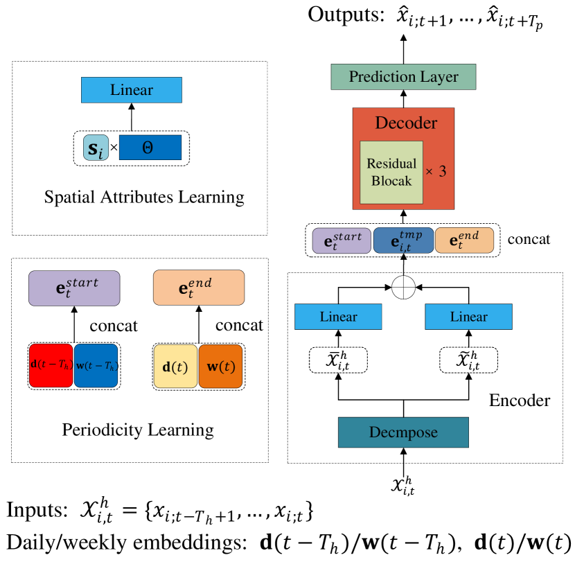
Figure 1: Overview of STLinear’s architecture

Linear Encoder

Time Series Decomposition.

Recent studies have demonstrated that simple linear models combined with decomposition techniques can achieve competitive or even superior performance against transformers on LSTF tasks (Zeng et al. 2023; Li et al. 2023; Ekambaram et al. 2023). Inspired by these findings, we incorporate a time series decomposition method to enhance our temporal dependency modeling.

For the $i$-th node, the $T_{h}$ historical observations at time-step $t$ are denoted as $\mathcal{X}^{h}_{i,t}=\{{x}_{i,t-T_{h}+1}\ldots,{x}_{i,t}\}\in\mathbb{R}^{T_{h}}$, which is further decomposed into a trend component $\mathcal{\overline{X}}^{h}_{i,t}\in\mathbb{R}^{T_{h}}$ and a remainder component $\mathcal{\tilde{X}}^{h}_{i,t}\in\mathbb{R}^{T_{h}}$ using a moving average kernel. These components are subsequently processed using two linear layers and a summation operation to compute the temporal embedding:

$$\overline{\mathbf{e}}_{i,t} =\mathbf{W}_{tr}\cdot\mathcal{\overline{X}}^{h}_{i,t}+\mathbf{b}_{{tr}}$$ (2)

$$\tilde{\mathbf{e}}_{i,t} =\mathbf{W}_{re}\cdot\mathcal{\tilde{X}}^{h}_{i,t}+\mathbf{b}_{{re}}$$ (3)

$$\mathbf{e}^{tmp}_{i,t} =\overline{\mathbf{e}}_{i,t}+\tilde{\mathbf{e}}_{i,t}$$ (4)

In these equations, $\overline{\mathbf{e}}_{i,t}$, $\tilde{\mathbf{e}}_{i,t}$, and $\mathbf{e}^{tmp}_{i,t}$ all possess a dimension of $\mathbb{R}^{d}$. Here, $d$ is a modifiable hyperparameter dictating the volume of encoded information. $\mathbf{W}_{tr},\mathbf{W}_{re}\in\mathbb{R}^{d\times T_{h}}$ and $\mathbf{b}_{tr},\mathbf{b}_{re}\in\mathbb{R}^{d}$ are the learnable model weights and biases of the linear layers.

Spatial Attributes Learning.

In Equations (2) and (3), the learnable parameters $\mathbf{W}_{tr}$, $\mathbf{W}_{re}$, $\mathbf{b}_{tr}$, and $\mathbf{b}_{re}$ are indeed $i$-invariant, i.e., shared between all nodes. However, traffic data from various nodes often manifest diverse patterns. Solely sharing parameters among nodes does not address the unique characteristics of each node based on their spatial locations, which can result in suboptimal predictions.

Exclusively assigning distinct sets of parameters to every node, however, might not be the optimal solution either. Research has shown that knowledge sharing across nodes can enhance both inference accuracy and efficiency (Bai et al. 2020). Given the limited data available for each node, sharing knowledge among nodes—akin to multitask learning paradigms—can elevate the overall inference accuracy.

To strike a balance between these two aspects, we adjust Equations (2) and (3) by introducing a spatial embedding vector $\mathbf{s}_{i}\in\mathbb{R}^{e}$ for each node:

$$\overline{\mathbf{e}}_{i,t} =(\Theta_{tr}\mathbf{s}_{i})\mathcal{\overline{X}}^{h}_{i,t}+\mathbf{\beta}_{tr}\mathbf{s}_{i}$$ (5)

$$\tilde{\mathbf{e}}_{i,t} =(\Theta_{re}\mathbf{s}_{i})\mathcal{\overline{X}}^{h}_{i,t}+\mathbf{\beta}_{re}\mathbf{s}_{i}$$ (6)

Here, $\Theta_{{tr}},\Theta_{{re}}\in\mathbb{R}^{d\times T_{h}\times e}$ and $\beta_{tr}$, $\beta_{re}\in\mathbb{R}^{d\times e}$ serve as learnable parameter pools. The hyperparameter $e$ decides the total number of parameters in these pools. Effective model parameters for each node are derived by multiplying the corresponding embedding $\mathbf{s}_{i}$ with the parameter pools, extracting the node-specific weights $\Theta_{tr}\mathbf{s}_{i},\Theta_{re}\mathbf{s}_{i}\in\mathbb{R}^{d\times T_{h}}$ and biases $\mathbf{\beta}_{tr}\mathbf{s}_{i},\mathbf{\beta}_{re}\mathbf{s}_{i}\in\mathbb{R}^{d}$. Importantly, this computation is only performed post-training, ensuring no additional computational load during inference. Moreover, these node-specific spatial embeddings encapsulate the spatial attributes yet bypassing the need to model inter-node spatial dependencies. This frees the model completely from the necessity of inter-node data-exchange during inference.

Periodicity Learning.

Urban activities heavily influence traffic data, resulting in discernible periodicity patterns such as morning and evening rushes. To capture time-of-the-day and day-of-the-week patterns, we introduce two sets of learnable vectors: $\mathbf{d}_{1},\dots,\mathbf{d}_{N_{d}}\in\mathbb{R}^{c}$ (where $N_{d}$ represents the number of time-steps per day) and $\mathbf{w}_{1},\dots,\mathbf{w}_{7}\in\mathbb{R}^{c}$. The hyperparameter $c$ is used for controlling the precision of the encoding. For a time-step $t$, the corresponding vector is denoted as $\mathbf{d}(t)$ and $\mathbf{w}(t)$, respectively.

Leveraging the two sets of vector which encode time-of-the-day and day-of-the-week information, we passes the initial and the terminal time of a given input $\mathcal{X}^{h}_{i,t}$ to the model using the initial time vector and the terminal time vector

$$\mathbf{e}^{start}_{t} =[\mathbf{d}(t-T_{h});\mathbf{w}(t-T_{h})]$$ (7)

$$\mathbf{e}^{end}_{t} =[\mathbf{d}(t);\mathbf{w}(t)]$$ (8)

Here, $[\cdot;\cdot]$ denotes vector concatenation.

Combining Embeddings.

Finally, integrating all the aforementioned embedding vectors (4), (7), and (8) which encode temporal information and spatial attributes, we derive the final embedding vector:

$$\mathbf{e}_{i,t}=[\mathbf{e}^{start}_{t};\mathbf{e}^{tem}_{i,t};\mathbf{e}^{end}_{t}]\in\mathbb{R}^{{(d+4c)}}$$ (9)

Linear Decoder

Our decoder employs a multi-layer structure featuring residual blocks. For the $l$-th layer:

$$\mathrm{Fc}(\mathbf{y}^{l-1}_{i,t}) =\mathbf{W}_{B}^{l}(\sigma(\mathbf{W}_{A}^{l}\mathbf{y}^{l-1}_{i,t}+\mathbf{b}_{A}^{l}))+\mathbf{b}^{l}_{B}$$ (10)

$$\mathrm{Res}(\mathbf{y}^{l}_{i,t}) =\mathrm{Fc}(\mathbf{y}^{l-1}_{i,t})+\mathbf{y}^{l-1}_{i,t}$$ (11)

In the above, $\mathbf{y}^{l}{i,t}$ represents the layer output of the $l$-th residual block of node $i$ at time-step $t$. The output of a decoder with $L$ residual blocks is denoted therefore as $\mathbf{y}_{i,t}^{L}$. We also define $\mathbf{y}^{0}_{i,t}=\mathbf{e}_{i,t}$, which is the encoder output in (9). $\mathbf{W}_{A}^{l}$, $\mathbf{W}_{B}^{l}$, $\mathbf{b}^{l}_{A}$, and $\mathbf{b}^{l}_{B}$ are learnable parameters for fully connected layers and are shared among nodes. $\sigma(\cdot)$ is the activation function, for which we primarily use Gaussian Error Linear Unit (GELU) in this paper.

To make $T_{p}$-step predictions, we incorporate one extra linear layer as the output layer:

$$\left\{{\hat{x}}_{i,t+1},\ldots,{\hat{x}}_{i,t+T_{p}}\right\}=\mathbf{W}_{p}\mathbf{y}_{i,t}^{L}+\mathbf{b}_{p}$$ (12)

The final output $\left\{{\hat{x}}_{i,t+1},\ldots,{\hat{x}}_{i,t+T_{p}}\right\}\in\mathbb{R}^{T_{p}}$ serves as the prediction of $\left\{{x}_{i,t+1},\ldots,{x}_{i,t+T_{p}}\right\}$.

Table 1: Summary of datasets used in experiments.

Datasets	#Nodes	Range
PEMS03	358	09/01/2018 - 30/11/2018
PEMS04	307	01/01/2018 - 28/02/2018
PEMS07	883	01/07/2017 - 31/08/2017
PEMS08	170	01/07/2016 - 31/08/2016

Evaluations

Datasets and metrics

Table 2: Overall prediction performance of different methods on the PEMS03, PEMS04, PEMS07 and PEMS08 dataset, the best results are highlighted in bold. (smaller value means better performance)

Dataset	Horizon	12			48			192			288
	Method	MAE	RMSE	MAPE	MAE	RMSE	MAPE	MAE	RMSE	MAPE	MAE	RMSE	MAPE
PEMS03	DLinear	21.18	37.67	20.22%	27.16	60.71	28.13%	39.20	59.98	28.22%	38.64	58.72	28.13%
	GraphWavenet	19.85	32.94	19.31%	23.14	37.40	21.64%	25.00	42.71	23.89%	24.89	42.74	23.76%
	DCRNN	17.99	30.31	18.34%	28.07	45.00	27.93%	28.36	45.76	26.56%	29.69	48.03	26.79%
	AGCRN	16.03	28.52	14.65%	19.68	37.29	22.38%	22.27	41.62	25.03%	23.49	43.15	25.29%
	STGNCDE	15.47	28.09	15.76%	22.36	39.92	21.66%	23.56	41.73	22.87%	23.93	44.93	22.91%
	GMAN	15.11	28.63	15.72%	20.45	33.85	20.98%	23.98	41.35	22.81%	N/A	N/A	N/A
	SSTBAN	N/A	N/A	N/A	N/A	N/A	N/A	N/A	N/A	N/A	N/A	N/A	N/A
	PDFormer	14.79	25.40	15.34%	19.89	32.75	19.59	N/A	N/A	N/A	N/A	N/A	N/A
	STID	15.20	25.20	16.09%	19.82	34.80	21.06%	22.22	40.96	23.50%	23.01	42.34	25.33%
	STLinear	14.73	25.33	14.62%	19.22	32.03	20.00%	21.81	40.51	22.33%	22.49	41.73	22.53%
PEMS04	DLinear	28.95	47.31	21.22%	39.29	60.71	28.13%	39.20	59.98	28.22%	38.64	58.72	28.13%
	GraphWavenet	22.24	30.59	16.51%	26.40	40.60	18.99%	28.63	44.36	19.98%	29.17	44.27	20.01%
	DCRNN	19.71	31.43	13.54%	23.70	36.42	15.23%	26.78	41.40	16.10%	27.24	40.85	16.21%
	AGCRN	19.83	32.30	12.97%	24.18	38.26	16.31%	26.65	41.89	16.33%	26.73	42.26	16.14%
	STGNCDE	19.21	31.09	12.76%	23.79	37.62	16.01%	27.37	41.88	17.81%	29.19	42.62	18.01%
	GMAN	19.14	31.60	13.20%	23.35	47.85	17.98%	25.02	50.68	18.93%	25.35	50.85	17.74%
	SSTBAN	22.63	38.24	14.69%	21.66	35.51	15.90%	N/A	N/A	N/A	N/A	N/A	N/A
	PDFormer	18.32	29.97	11.87%	21.19	34.67	14.46%	N/A	N/A	N/A	N/A	N/A	N/A
	STID	18.29	29.82	12.49%	21.04	34.04	14.51%	23.20	38.51	16.44%	23.78	39.99	16.79%
	STLinear	18.21	29.89	11.87%	20.54	33.97	13.66%	22.32	38.13	15.17%	23.24	39.87	15.66%
PEMS07	DLinear	30.29	49.63	14.36%	42.17	63.45	22.51%	42.09	63.14	22.43	41.05	63.28	22.07%
	GraphWavenet	20.65	33.49	8.91%	24.16	40.19	10.34%	26.82	45.73	11.58%	26.91	46.69	11.44%
	DCRNN	25.22	38.61	11.82%	27.48	41.31	12.53%	30.23	45.86	13.73%	34.26	53.20	15.38%
	AGCRN	22.37	36.55	9.12%	26.10	42.78	12.03%	30.28	49.53	14.20%	31.10	49.78	14.36%
	STGNCDE	20.53	33.84	8.80%	30.34	48.75	13.33%	35.83	55.79	14.97%	36.64	56.75	15.13%
	GMAN	20.43	33.30	8.69%	23.78	40.15	10.25%	25.87	46.45	11.78%	N/A	N/A	N/A
	SSTBAN	N/A	N/A	N/A	N/A	N/A	N/A	N/A	N/A	N/A	N/A	N/A	N/A
	PDFormer	19.83	32.87	8.40%	23.25	41.14	10.08%	N/A	N/A	N/A	N/A	N/A	N/A
	STID	19.54	32.85	8.25%	23.49	40.05	10.52%	26.14	48.87	11.92%	26.50	48.10	11.97%
	STLinear	19.19	32.47	8.07%	22.63	39.05	9.73%	25.18	44.56	11.57%	25.57	45.89	11.41%
PEMS08	DLinear	21.41	30.34	15.95%	31.99	46.17	22.55%	32.38	47.28	22.69%	32.99	47.39	22.63%
	GraphWavenet	16.63	26.03	10.42%	18.59	30.27	11.63%	18.73	31.24	13.95%	19.04	31.38	13.97%
	DCRNN	18.19	28.18	11.24%	18.60	30.04	12.66%	22.82	35.67	14.73%	23.27	36.94	15.10%
	AGCRN	15.95	25.22	10.09%	17.45	28.05	11.25%	21.17	32.86	14.83%	21.96	33.41	12.98%
	STGNCDE	15.45	24.81	10.18%	21.18	33.46	13.69%	23.28	37.13	14.91%	24.57	38.56	15.60%
	GMAN	15.31	24.92	10.13%	18.70	35.89	16.81%	20.21	35.89	18.66%	20.86	40.84	18.82%
	SSTBAN	18.37	24.87	10.59%	16.94	28.82	12.47%	20.07	32.32	14.29%	20.34	33.40	14.20%
	PDFormer	13.58	23.51	9.05%	16.91	28.28	11.74%	18.61	31.17	13.72%	19.63	32.57	14.19%
	STID	14.20	23.49	9.28%	16.89	27.02	11.67%	18.86	31.24	13.30%	19.14	31.94	13.81%
	STLinear	13.95	23.39	9.21%	16.52	27.63	10.87%	17.97	30.37	12.47%	18.29	31.26	12.87%

To assess the performance of the proposed STLinear, we carried out comprehensive experiments using four widely recognized real-world traffic benchmark datasets: PEMS03, PEMS04, PEMS07, and PEMS08 (Chen et al. 2001). Detailed descriptions of these datasets can be found in Table 1.

We partitioned each dataset using a 6:2:2 split for training, validation, and testing purposes, respectively. Traffic flows were aggregated at 5-minute intervals. To provide a thorough evaluation of STLinear for both short-term and long-term traffic prediction, we examined four prediction scenarios where $T_{h}=T_{p}\in\{12,48,192,288\}$. Our performance metrics included the Root Mean Square Error (RMSE), Mean Absolute Error (MAE), and Mean Absolute Percentage Error (MAPE).

Baselines and configurations

Baselines.

We compare STLinear with following baselines: DLinear (Zeng et al. 2023), Graph Wavenet (Wu et al. 2019), AGCRN (Bai et al. 2020), STG-NCDE (Choi et al. 2022), GMAN (Zheng et al. 2020), SSTBAN (Guo et al. 2023), PDFormer (Jiang et al. 2023), and STID (Shao et al. 2022). DLinear represents a linear-based approach for long time series forecasting. Graph Wavenet is a notable CNN-based STGNN. Meanwhile, DCRNN, AGCRN, and STG-NCDE are RNN-based STGNNs. GMAN, SSTBAN, and PDFormer are Transformer-based STGNNs. Notably, SSTBAN is the state-of-the-art STGNN for long-term traffic prediction, while PDFormer excels in short-term forecasting. STID is the state-of-the-art linear-based approach for traffic prediction.

Configurations.

For all datasets, models were trained over 300 epochs using the Adam optimizer (Kingma and Ba 2015). The learning rate was set to 2e-4, with a batch size of 32. Hyperparameter $d$ was configured at 32, $e$ at 8, and $c$ at 32. The decoder has $L=3$ residual blocks. The moving average kernel size was optimized from among ${3,5,15,25}$. All evaluations are implemented and executed on workstations equipped with NVIDIA A100 GPU. For all baseline models, we proceed as follows:

• If experimental results for a specific scenario are not available, we execute their codes using default configurations.

• When official results are available, we directly cite these findings.

However, there are exceptions. The execution of PDFormer and GMAN’s code on certain scenarios resulted in out-of-memory errors, rendering their results inapplicable for those scenarios. Furthermore, while SSTBAN employs a unique data-preprocessing technique, it does not furnish the processed PEMS03 and PEMS07 datasets. Consequently, we were unable to evaluate SSTBAN on these two datasets using its original source code. For our evaluations, we reported the average outcomes derived from five separate runs.

Inference Accuracy

In Table 2, we present an exhaustive evaluation of all baseline methods alongside STLinear, tested on four distinct datasets across forecast horizons of 12, 48, 192, and 288. Our analysis leads to the following observations:

• Across nearly all datasets and scenarios, STLinear consistently delivers top-tier performance. An exception to this trend is the PEMS08-12 scenario. Nonetheless, STLinear remains the leading model in the majority of scenarios for the PEMS08 dataset.

• Compared to DLinear, STGNN-based methods display a pronounced edge. We hypothesize this advantage arises because STGNNs harness the power of GNNs to identify spatial interdependencies among traffic series. Conversely, DLinear overlooks these spatial dependencies, making it less adept at handling the intricacies of traffic data. On the contrary, however, STLinear outperforms STGNN-based baselines even without explicitly modeling these spatial dependencies. This suggests the possibility that emphasizing spatial dependencies might not be quintessential. Learning only spatial attributes could potentially serve as a more efficient alternative to GNNs.

• STLinear excels in both short-term and long-term traffic forecasting, outpacing competing methodologies. This highlights that even in the absence of sophisticated sequential models like Transformers, leveraging conventional time series decomposition techniques and embedding temporal patterns (time-of-the-day and day-of-the-week information) within simple linear layers can effectively discern the temporal correlations in traffic data.

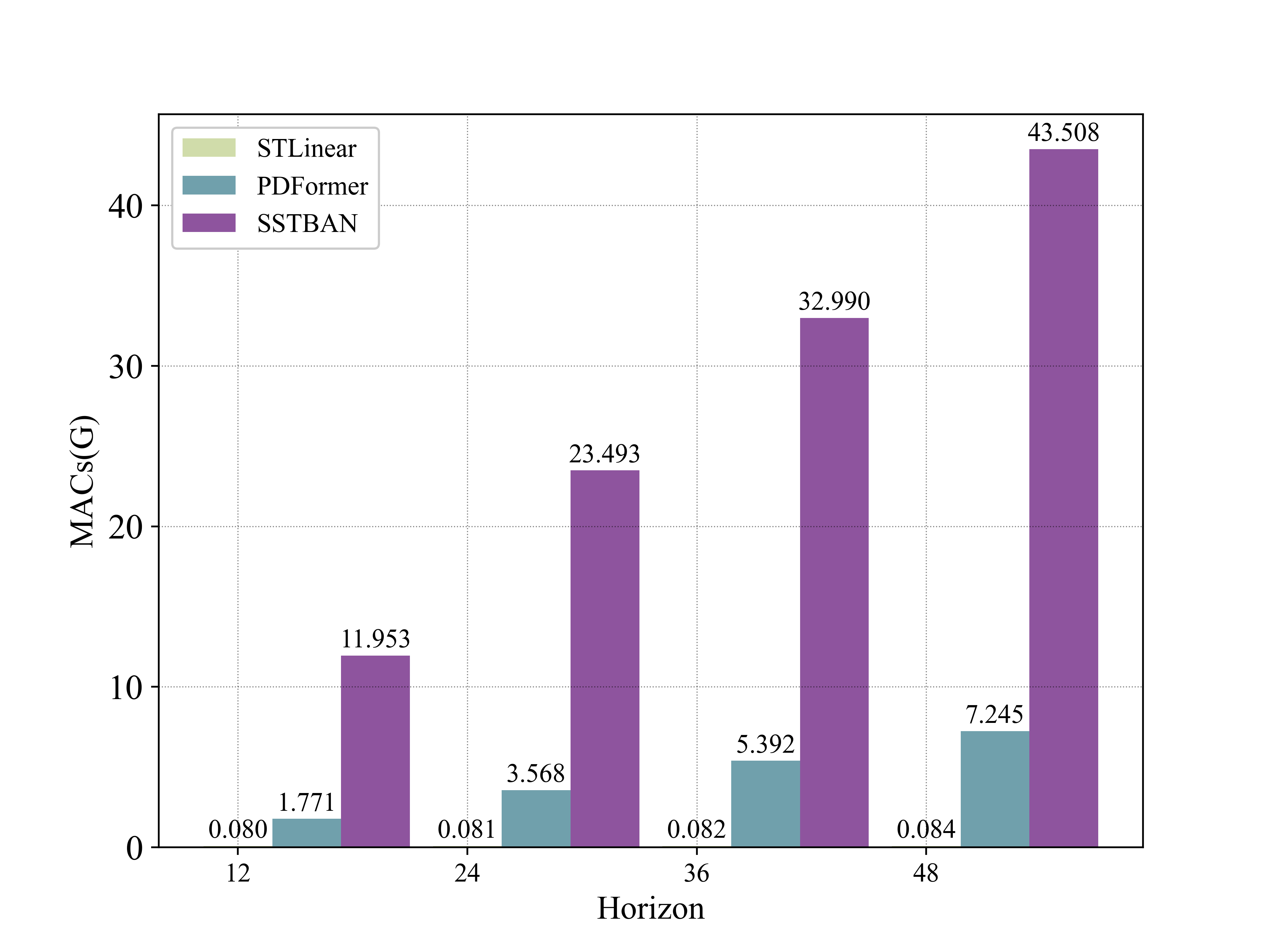
(a) MACs/epoch with different prediction horizon length.

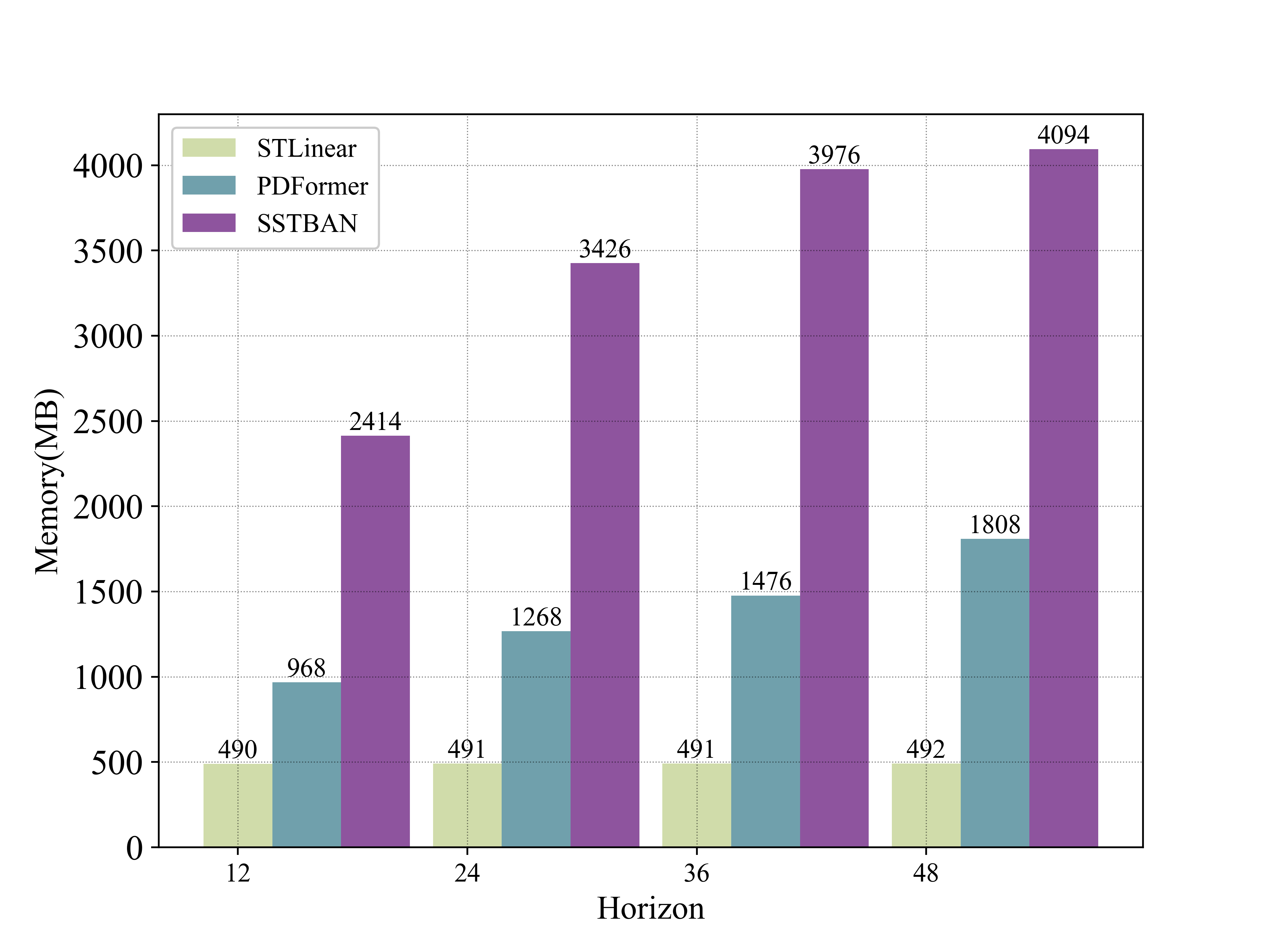
(b) Memory cost with different prediction horizon length.

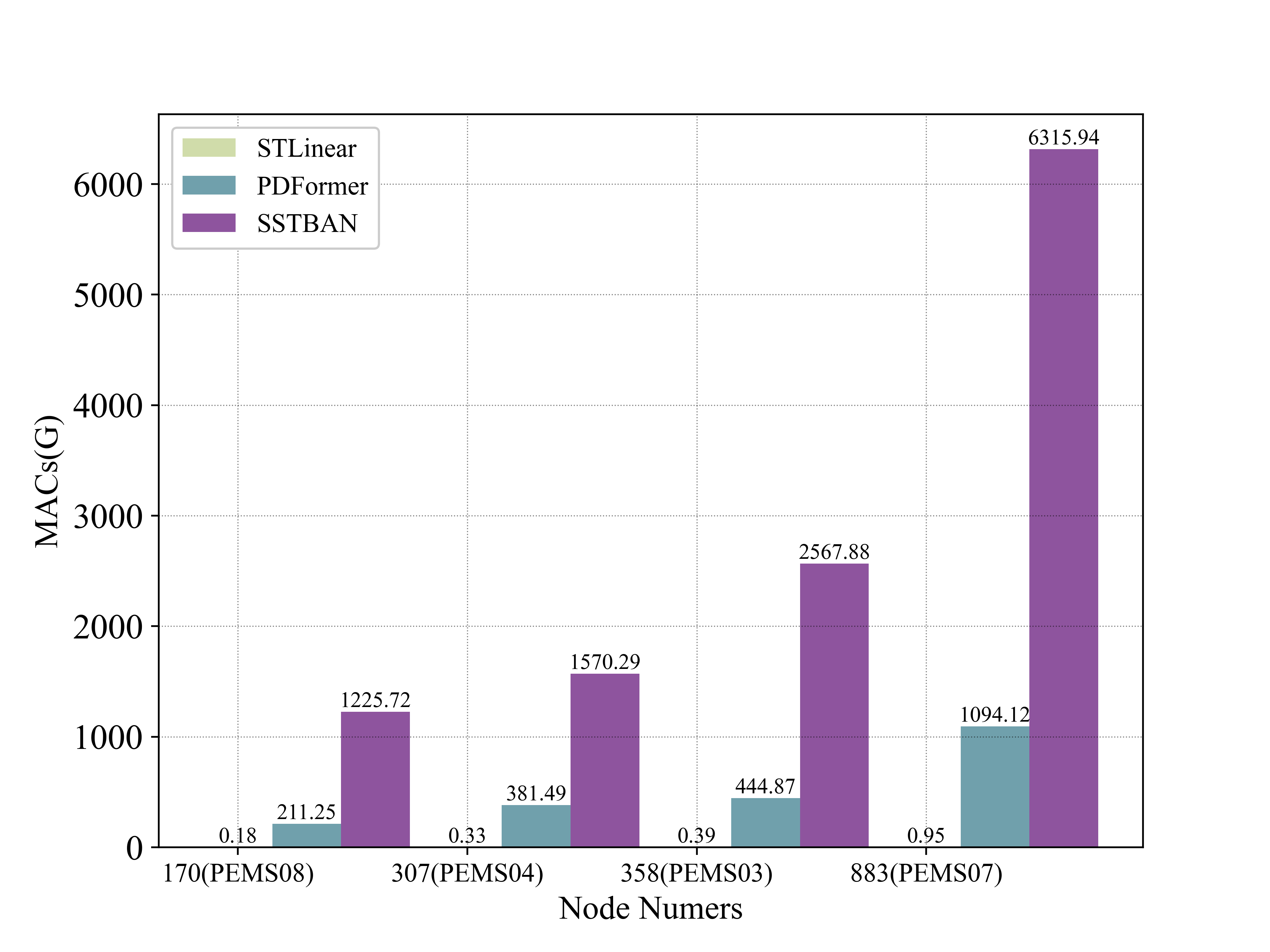
(c) MACs/epoch with different numbers of node.

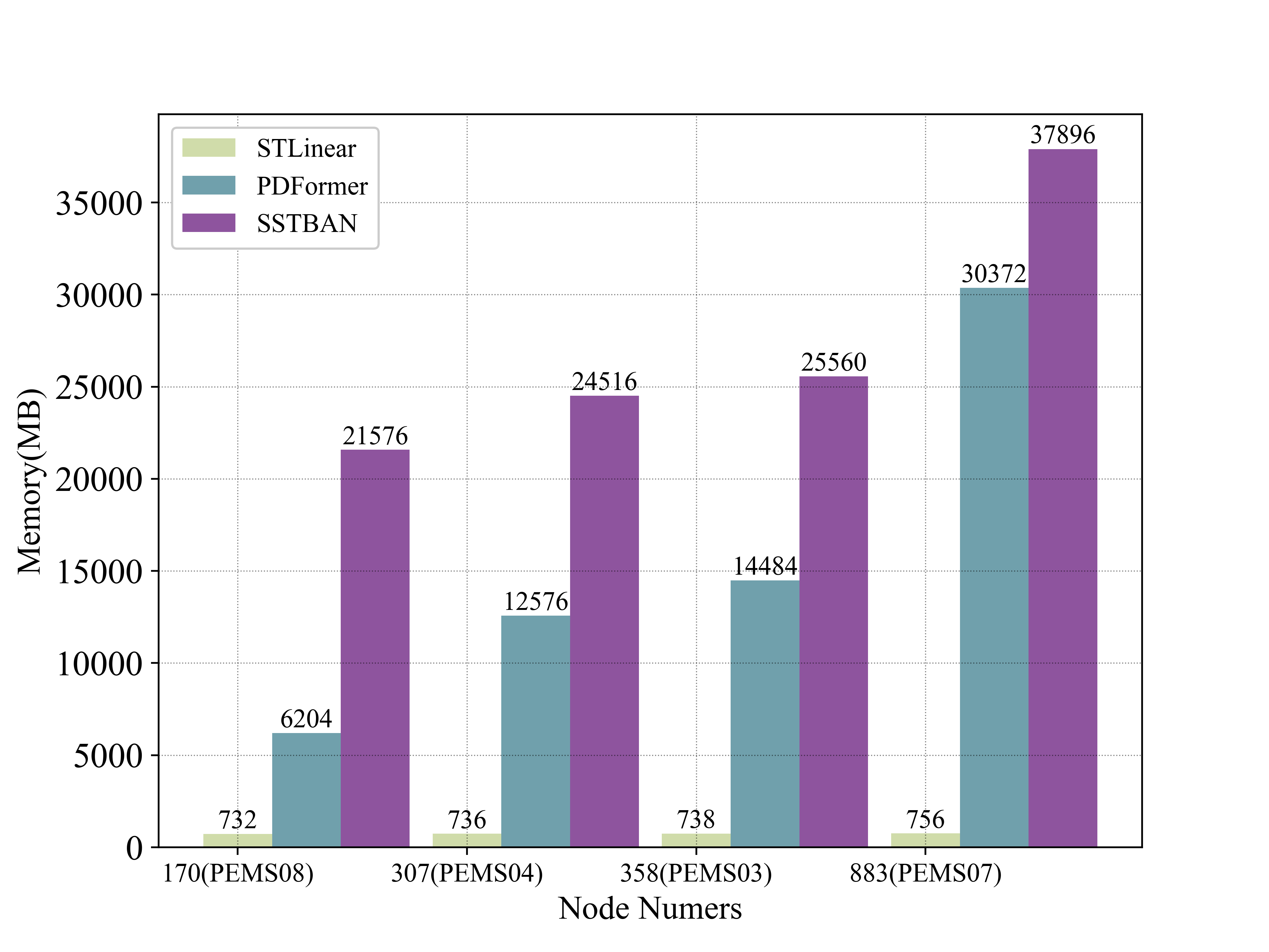
(d) Memory cost with different numbers of node.

Figure 2: (a) MACs per epoch for inference on dataset PEMS04 with prediction horizon length $\{12,24,36,48\}$; (b) Memory cost for the same setup as (a); (c) MACs per epoch for inference on four different datasets containing 170, 307, 358 and 883 nodes, respectively. The prediction horizon length is fixed to 288; (d) Memory cost for the same setup as (c)

Efficiency

Table 3: MACs per epoch and memory cost for training with prediction horizon length of $\{12,48,192,288\}$.

Dataset	Method		12	48	192	288
PEMS04	PDFormer	MACs(G)/epoch	4.64e+4($22.1\times$)	1.89e+5($86.7\times$)	N/A	N/A
		Memory(MB)	5.83e+3($2.6\times$)	2.32e+4($10.1\times$)	OOM	OOM
	SSTBAN	MACs(G)/epoch	2.23e+5($105.9\times$)	8.09e+5($371.0\times$)	N/A	N/A
		Memory(MB)	4.31e+3($1.9\times$)	1.65e+4($7.2\times$)	OOM	OOM
	STLinear	MACs(G)/epoch	2.10e+3($1\times$)	2.18e+3($1\times$)	2.48e+3($1\times$)	2.68e+3($1\times$)
		Memory(MB)	2.27e+3($1\times$)	2.30e+3($1\times$)	2.43e+3($1\times$)	2.59e+3($1\times$)
PEMS08	PDFormer	MACs(G)/epoch	2.70e+4($22.1\times$)	1.10e+5($79.5\times$)	1.35e+5($93.6\times$)	6.57e+6(4209.7$\times$)
		Memory(MB)	2.61e+3($1.2\times$)	8.83e+3($4.0\times$)	2.71e+4($11.8\times$)	4.77e+4($20.5\times$)
	SSTBAN	MACs(G)/epoch	1.99e+5($162.3\times$)	6.64e+5($523.1\times$)	3.37e+6($2232.6\times$)	3.81e+7($24425.6\times$)
		Memory(MB)	3.68e+3($1.7\times$)	8.93e+3($4.1\times$)	3.12e+4($13.6\times$)	4.84e+4($20.5\times$)
	STLinear	MACs(G)/epoch	1.22e+3($1\times$)	1.27e+3($1\times$)	1.45e+3($1\times$)	1.56e+3($1\times$)
		Memory(MB)	2.19e+3($1\times$)	2.20e+3($1\times$)	2.30e+3($1\times$)	2.32e+3($1\times$)

Efficiency, one of the major motivation for the designing of STLinear, critically influences the practicality of deep-learning-enabled traffic prediction methods. STLinear has a time complexity of $\mathcal{O}(N)$. In other words, the computational expense of STLinear increases linearly with the number of nodes in the traffic network, far superior than the STGNN-based baselines with a quadratic time complexity $\mathcal{O}(N^{2})$.

Apart from the theoretical time complexity, we empirically evaluated the training and inference efficiencies of STLinear against two state-of-the-art models: SSTBAN and PDFormer. Table 3 provides a summary of the training efficiency on PEMS04 and PEMS08 datasets, while Figure. 2 illustrates the influence of prediction horizon length $T_{p}$ and node count $N$ on inference efficiency. Both during training and inference, STLinear stands out as the most efficient model. For example, in a direct comparison with SSTBAN (state-of-the-art method published in 2023), STLinear showcases a notable reduction in computational demands. Specifically, there’s a reduction of 95.50% to 99.81% in MACs per epoch and 49.38% to 98.01% in memory usage. These efficiencies become even more evident during the training phase, with reductions ranging from 99.10% to 99.96% in MACs per epoch and 15.99% to 95.20% in memory usage.

It is pertinent to note that, during our evaluations on a platform equipped with 80 GB of graphic memory, both SSTBAN and PDFormer faced out-of-memory issues when tested on the PEMS04-192 and PEMS04-288 configurations. This observation underscores potential limitations in deploying Transformer-based models in extensive traffic prediction scenarios.

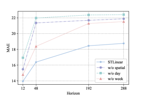
(a) MAE

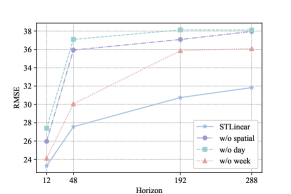
(b) RMSE

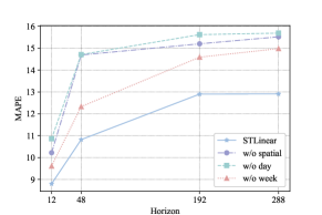
(c) MAPE

Figure 3: Inference accuracy of STLinear against the three variants for the ablation study. Evaluated on PEMS08 dataset.

Contribution of Spatial Attributes and Periodicity

In this section, we conduct ablation studies to validate the contributions of the three embedding vectors: (i) the spatial embedding $\mathbf{s}_{i}$ modeling the spatial attributes; (ii) the time-of-the-day embedding $\mathbf{d}(t)$; (iii) the day-of-the-week embedding $\mathbf{w}(t)$. We assess STLinear against the following three model variants:

1. w/o spatial embedding $\mathbf{s}_{i}$: This variant omits the spatial embedding $\mathbf{s}_{i}$, implying that all nodes share the same parameters. Consequently, it cannot capture distinct spatial attributes associated with each node.

2. w/o time-of-the-day embedding $\mathbf{d}(t)$: This variant excludes the time-of-the-day embedding $\mathbf{d}(t)$ from both initial time vector $\mathbf{e}^{start}_{t}$ the terminal time vector $\mathbf{e}^{end}_{t}$.

3. w/o day-of-the-week embedding $\mathbf{w}(t)$: Similarly, this omits the day-of-the-week embedding $\mathbf{w}(t)$ from both initial time vector $\mathbf{e}^{start}_{t}$ the terminal time vector $\mathbf{e}^{end}_{t}$.

The comparative performance of these variants on the PEMS08 datasets is illustrated in Figure. 3. From our findings, we infer the following:

• Overall, STLinear consistently achieves better results than all other variants, showing that the inclusion of the spatial attributes learning and periodicity information indeed enhances the model’s capabilities.

• In every scenario, the absence of the time-of-the-day embedding adversely affects the performance of STLinear. The w/o time-of-the-day embedding variant is consistently outperformed by other models, emphasizing that daily periodicity is a critical factor in traffic prediction.

• The w/o spatial embedding variant performs better than the w/o time-of-the-day embedding but falls short of the w/o day-of-the-week embedding. This suggests that the inability to learn spatial attributes has a more pronounced impact than the absence of weekly periodicity, but it’s less detrimental than missing daily periodicity.

Conclusion

Our study sought to address the limitations of the application of state-of-the-art STGNNs on traffic prediction tasks. Driven by recent findings, we pinpointed and advocated for three primary solutions to enhance efficiency: the emphasis on a node-embedding approach, the endorsement of time series decomposition, and the introduction of periodicity learning. To actualize these solutions, we introduced STLinear, a minimalist and innovative model architecture. Distinguished by its fully localized nature, STLinear eliminates the need for inter-node data exchanges during its operations, thus reducing computational overhead and providing a pathway for deployment in communication-restricted environments. The model’s reliance on pure linear layers further amplifies its computational efficiency.

Empirical analyses conducted on real-world datasets underscore the efficacy and efficiency of STLinear. Notably, it matches or surpasses established STGNNs in traffic prediction accuracy while drastically curtailing computational demands. Compared to the benchmark SSTBAN method, STLinear exhibited significant reductions in MACs per epoch during both training and inference stages, coupled with reduced memory consumption. In essence, our work underscores the potential of STLinear to serve as a streamlined, yet potent alternative to traditional STGNNs, offering a more efficient path forward for ITS and smart city development. In the larger canvas of traffic prediction research, our findings may potentially allow a paradigm shift. With models like STLinear, it is feasible to have the best of both worlds: robust predictive capabilities with streamlined computational requirements. As urban landscapes continue to evolve and as the demands on ITS grow, solutions like STLinear will prove invaluable in bridging the gap between theoretical advancements and practical implementations in real-world traffic management systems.

References

- Bai et al. (2020) Bai, L.; Yao, L.; Li, C.; Wang, X.; and Wang, C. 2020. Adaptive Graph Convolutional Recurrent Network for Traffic Forecasting. In Advances in Neural Information Processing Systems, 17804–17815. Red Hook, NY, USA: Curran Associates Inc.
- Chen et al. (2001) Chen, C.; Petty, K.; Skabardonis, A.; Varaiya, P.; and Jia, Z. 2001. Freeway Performance Measurement System: Mining Loop Detector Data. Transportation Research Record, 1748(1): 96–102.
- Chen et al. (2022) Chen, Y.; Segovia-Dominguez, I.; Coskunuzer, B.; and Gel, Y. R. 2022. TAMP-S2GCNets: Coupling Time-Aware Multipersistence Knowledge Representation with Spatio-Supra Graph Convolutional Networks for Time-Series Forecasting. In The Tenth International Conference on Learning Representations, ICLR 2022, Virtual Event, April 25-29, 2022.
- Chen, Segovia-Dominguez, and Gel (2021) Chen, Y.; Segovia-Dominguez, I.; and Gel, Y. R. 2021. Z-GCNETs: Time Zigzags at Graph Convolutional Networks for Time Series Forecasting. In Meila, M.; and Zhang, T., eds., Proceedings of the 38th International Conference on Machine Learning, ICML 2021, 18-24 July 2021, Virtual Event, volume 139 of Proceedings of Machine Learning Research, 1684–1694. PMLR.
- Choi et al. (2022) Choi, J.; Choi, H.; Hwang, J.; and Park, N. 2022. Graph Neural Controlled Differential Equations for Traffic Forecasting. In Thirty-Sixth AAAI Conference on Artificial Intelligence, AAAI 2022, Thirty-Fourth Conference on Innovative Applications of Artificial Intelligence, IAAI 2022, The Twelveth Symposium on Educational Advances in Artificial Intelligence, EAAI 2022 Virtual Event, February 22 - March 1, 2022, 6367–6374. AAAI Press.
- Connor, Atlas, and Martin (1992) Connor, J.; Atlas, L. E.; and Martin, D. R. 1992. Recurrent networks and NARMA modeling. In Advances in Neural Information Processing Systems, 301–308. Red Hook, NY, USA: Curran Associates Inc.
- Duan et al. (2023) Duan, W.; He, X.; Zhou, Z.; Thiele, L.; and Rao, H. 2023. Localised Adaptive Spatial-Temporal Graph Neural Network. In Proceedings of the 29th ACM SIGKDD Conference on Knowledge Discovery and Data Mining, KDD ’23, 448–458. New York, NY, USA: Association for Computing Machinery. ISBN 9798400701030.
- Ekambaram et al. (2023) Ekambaram, V.; Jati, A.; Nguyen, N.; Sinthong, P.; and Kalagnanam, J. 2023. TSMixer: Lightweight MLP-Mixer Model for Multivariate Time Series Forecasting. In Proceedings of the 29th ACM SIGKDD Conference on Knowledge Discovery and Data Mining, KDD ’23, 459–469. New York, NY, USA: Association for Computing Machinery. ISBN 9798400701030.
- Guo et al. (2019) Guo, S.; Lin, Y.; Feng, N.; Song, C.; and Wan, H. 2019. Attention Based Spatial-Temporal Graph Convolutional Networks for Traffic Flow Forecasting. In Proceedings of the AAAI Conference on Artificial Intelligence, 922–929. Palo Alto, CA, USA: AAAI Press.
- Guo et al. (2023) Guo, S.; Lin, Y.; Gong, L.; Wang, C.; Zhou, Z.; Shen, Z.; Huang, Y.; and Wan, H. 2023. Self-Supervised Spatial-Temporal Bottleneck Attentive Network for Efficient Long-term Traffic Forecasting. In 39th IEEE International Conference on Data Engineering, ICDE 2023, Anaheim, CA, USA, April 3-7, 2023, 1585–1596. IEEE.
- Huang et al. (2020) Huang, R.; Huang, C.; Liu, Y.; Dai, G.; and Kong, W. 2020. LSGCN: Long Short-Term Traffic Prediction with Graph Convolutional Networks. In Bessiere, C., ed., Proceedings of the Twenty-Ninth International Joint Conference on Artificial Intelligence, IJCAI 2020, 2355–2361. ijcai.org.
- Jiang et al. (2023) Jiang, J.; Han, C.; Zhao, W. X.; and Wang, J. 2023. PDFormer: Propagation Delay-Aware Dynamic Long-Range Transformer for Traffic Flow Prediction. In Williams, B.; Chen, Y.; and Neville, J., eds., Thirty-Seventh AAAI Conference on Artificial Intelligence, AAAI 2023, Thirty-Fifth Conference on Innovative Applications of Artificial Intelligence, IAAI 2023, Thirteenth Symposium on Educational Advances in Artificial Intelligence, EAAI 2023, Washington, DC, USA, February 7-14, 2023, 4365–4373. AAAI Press.
- Kingma and Ba (2015) Kingma, D. P.; and Ba, J. 2015. Adam: A method for stochastic optimization. In Proceedings of the International Conference on Learning Representations.
- Li and Zhu (2021) Li, M.; and Zhu, Z. 2021. Spatial-Temporal Fusion Graph Neural Networks for Traffic Flow Forecasting. In Proceedings of the AAAI Conference on Artificial Intelligence, 4189–4196. Palo Alto, CA, USA: AAAI Press.
- Li et al. (2018) Li, Y.; Yu, R.; Shahabi, C.; and Liu, Y. 2018. Diffusion Convolutional Recurrent Neural Network: Data-Driven Traffic Forecasting. In 6th International Conference on Learning Representations, ICLR 2018, Vancouver, BC, Canada, April 30 - May 3, 2018, Conference Track Proceedings. OpenReview.net.
- Li et al. (2023) Li, Z.; Rao, Z.; Pan, L.; and Xu, Z. 2023. MTS-Mixers: Multivariate Time Series Forecasting via Factorized Temporal and Channel Mixing. CoRR, abs/2302.04501.
- Makridakis and Hibon (1997) Makridakis, S.; and Hibon, M. 1997. ARMA models and the Box–Jenkins methodology. Journal of forecasting, 16(3): 147–163.
- Pan et al. (2019) Pan, Z.; Liang, Y.; Wang, W.; Yu, Y.; Zheng, Y.; and Zhang, J. 2019. Urban Traffic Prediction from Spatio-Temporal Data Using Deep Meta Learning. In Teredesai, A.; Kumar, V.; Li, Y.; Rosales, R.; Terzi, E.; and Karypis, G., eds., Proceedings of the 25th ACM SIGKDD International Conference on Knowledge Discovery & Data Mining, KDD 2019, Anchorage, AK, USA, August 4-8, 2019, 1720–1730. ACM.
- Shao et al. (2022) Shao, Z.; Zhang, Z.; Wang, F.; Wei, W.; and Xu, Y. 2022. Spatial-Temporal Identity: A Simple yet Effective Baseline for Multivariate Time Series Forecasting. In Hasan, M. A.; and Xiong, L., eds., Proceedings of the 31st ACM International Conference on Information & Knowledge Management, Atlanta, GA, USA, October 17-21, 2022, 4454–4458. ACM.
- Vaswani et al. (2017) Vaswani, A.; Shazeer, N.; Parmar, N.; Uszkoreit, J.; Jones, L.; Gomez, A. N.; Kaiser, Ł.; and Polosukhin, I. 2017. Attention is all you need. In Advances in Neural Information Processing Systems, 6000–6010. Red Hook, NY, USA: Curran Associates Inc.
- Wu et al. (2019) Wu, Z.; Pan, S.; Long, G.; Jiang, J.; and Zhang, C. 2019. Graph Wavenet for Deep Spatial-Temporal Graph Modeling. In Proceedings of the 28th International Joint Conference on Artificial Intelligence, IJCAI’19, 1907–1913. AAAI Press. ISBN 9780999241141.
- Yu, Yin, and Zhu (2018) Yu, B.; Yin, H.; and Zhu, Z. 2018. Spatio-Temporal Graph Convolutional Networks: A Deep Learning Framework for Traffic Forecasting. In Proceedings of the International Joint Conference on Artificial Intelligence, 3634–3640. Burlington, MA, USA: Morgan Kaufmann.
- Zeng et al. (2023) Zeng, A.; Chen, M.; Zhang, L.; and Xu, Q. 2023. Are Transformers Effective for Time Series Forecasting? In Williams, B.; Chen, Y.; and Neville, J., eds., Thirty-Seventh AAAI Conference on Artificial Intelligence, AAAI 2023, Thirty-Fifth Conference on Innovative Applications of Artificial Intelligence, IAAI 2023, Thirteenth Symposium on Educational Advances in Artificial Intelligence, EAAI 2023, Washington, DC, USA, February 7-14, 2023, 11121–11128. AAAI Press.
- Zhang et al. (2022) Zhang, T.; Zhang, Y.; Cao, W.; Bian, J.; Yi, X.; Zheng, S.; and Li, J. 2022. Less is more: Fast multivariate time series forecasting with light sampling-oriented mlp structures. arXiv preprint arXiv:2207.01186.
- Zheng et al. (2020) Zheng, C.; Fan, X.; Wang, C.; and Qi, J. 2020. GMAN: A Graph Multi-Attention Network for Traffic Prediction. In The Thirty-Fourth AAAI Conference on Artificial Intelligence, AAAI 2020, The Thirty-Second Innovative Applications of Artificial Intelligence Conference, IAAI 2020, The Tenth AAAI Symposium on Educational Advances in Artificial Intelligence, EAAI 2020, New York, NY, USA, February 7-12, 2020, 1234–1241. AAAI Press.
- Zhou et al. (2021) Zhou, H.; Zhang, S.; Peng, J.; Zhang, S.; Li, J.; Xiong, H.; and Zhang, W. 2021. Informer: Beyond Efficient Transformer for Long Sequence Time-Series Forecasting. In Thirty-Fifth AAAI Conference on Artificial Intelligence, AAAI 2021, Thirty-Third Conference on Innovative Applications of Artificial Intelligence, IAAI 2021, The Eleventh Symposium on Educational Advances in Artificial Intelligence, EAAI 2021, Virtual Event, February 2-9, 2021, 11106–11115. AAAI Press.
- Zivot and Wang (2006) Zivot, E.; and Wang, J. 2006. Vector autoregressive models for multivariate time series. Modeling financial time series with S-PLUS®, 385–429.