Age of Information in a Multisource Ber/Geo/1/1 Preemptive Queueing System

Abstract

This work studies the information freshness of the vehicle-to-infrastructure status updating in Internet of vehicles, which is modeled as a multi-source Ber/Geo/1/1 preemptive queueing system with heterogeneous service time. We pay attention to both the distribution and average of AoI. To fully track the per-source AoI evolution, a Markov two-dimensional (2D) age process is introduced. The first element of the 2D age process stands for the instantaneous per-source AoI, while the second represents whether an update of the concerned source is being served and its current age. A complete framework and detailed analyses on the per-source AoI are presented based on the Markovity of the 2D age process. By studying the state transition probabilities, stationary equations, and stationary distribution of the 2D age process, analytical expressions of the probability mass function and average of per-source AoI are derived. Numerical results validate the accuracy of the theoretical analyses.

I Introduction

Internet of vehicles (IoV) is in accelerating development with the rapid advances of sensing, communication, computation and artificial intelligence technologies. In IoV, the vehicle-to-infrastructure (V2I) communication provides the real-time vehicle status updating, facilitating the timely vehicular-data-driven analysis and decision-making at the roadside infrastructure (RI)[1]. In effect, the V2I link is usually extracted as a real-time wireless status updating system consisting of multiple information sources, a transmitter and a monitor[2]. Information freshness becomes one of the critical indicators in the V2I link. Age of information (AoI), which is defined as the time elapsed since the latest successfully received update of a concerned source was generated, is pertinent to characterize the information freshness for the status updating system[3].

Queueing systems are effective to model the wireless status updating systems, providing abundant insights for improving the information freshness[4, 5, 6, 7, 8, 9, 10, 11, 12, 13, 14, 15, 16]. In particular, multi-source queueing systems are more appropriate and accurate for modeling the status updating of the V2I link, since there are often multiple kinds of vehicular status, e.g. velocity, acceleration and surrounding object information, required to report to the RI[4]. For queueing systems, most existing works adopted the average AoI, i.e, expectation or time-average of the AoI process to evaluate the information freshness[5, 6, 7, 8]. For instance, average AoIs in the single- and multi-source M/G/1/1 preemptive and non-preemptive systems were derived in [5, 6, 7]. For discrete-time queueing systems, the average AoIs in single-source Ber/G/1 first-come-first-served (FCFS), G/G/1/1 preemptive and G/G/$\infty$ systems were established in [8].

To characterize the information freshness comprehensively, some recent works focused on studying the (stationary) distribution of AoI[9, 10, 11, 12, 13, 14, 15, 16]. For continuous-time queueing systems, the methods for deriving the distribution of AoI mainly include the stochastic hybrid systems (SHS) approach [9] and the sample-path (SP) approach[10, 11, 12]. The distributions of AoIs in the single- and multi-source M/G/1/1 preemptive and non-preemptive systems were investigated by using the SP approach in[10, 11, 12]. In contrast, the two-dimensional (2D) age process approach[13, 14] and the SP approach[15] are two main methods for analysing the distributions of AoI in discrete-time queueing systems. In particular, the 2D age process introduces a 2D Markov age process to fully track the AoI evolution, which can be seen as a generalization of the SHS approach[14]. The first element of the 2D age process stands for the age process at the monitor, while the second represents the age of the update being served. Compared with the SP approach, the AoI evolution is presented more visually by utilizing the 2D age process approach, facilitating to study the statistical characteristics of the AoI thoroughly. With the help of the 2D age process, the distributions of AoIs in the single-source Ber/Geo/1 FCFS and Ber/G/1/1 non-preemptive systems were derived in [13, 14] respectively. Moreover, an algorithm based on the discrete-time Markov chain (DTMC) theory was proposed to numerically obtain the distributions of per-source AoIs in multi-source bufferless preemptive and non-preemptive systems with Bernoulli arrivals and discrete phase-type service times[16].

Thorough studies on the information freshness in the V2I link are necessary due to highly dynamic nature of the vehicle status. However,to the best of our knowledge, the statistical characteristics of AoI (which are key to many extended studies[12]) in the discrete-time multi-source queueing system (which can model the V2I link effectively) have not been sufficiently studied. To fill this gap, we study the AoI in a V2I link with multiple information sources, a vehicle of bufferless transmitter, retransmission protocol and preemption queueing policy, which is modeled as a multi-source Ber/Geo/1/1 preemptive system with the source-dedicated service time, and focus on the probability mass function (p.m.f.) and average of AoI. The main contributions of this work are summarized as follows.

• We extend the 2D age process approach into the discrete-time multi-source queueing system, and present the complete and detailed analyses on the per-source AoI evolution based on the Markovity of the 2D age process.

• The analytical expressions of the p.m.f. and average of the per-source AoI are derived. The AoI performance versus all system parameters and the effect of the retransmission protocol are analysed by numerical results.

Specifically, similar to the approach in single-source systems, we define the first element of the 2D age process as the per-source AoI process. To fit the 2D age process approach into the multi-source bufferless preemptive system and simplify the analysis, we let the second element represent whether an update of the concerned source is in transmission and its current age, while ignoring the link details when no concerned-source update is being transmitted. The Markovity of the 2D age process helps overcome the challenge for analysing the frequently disturbed queuing process caused by the preemption among sources. By analysing state transitions of the 2D age process, we further establish the stationary equations, through which the stationary distribution of the 2D age process is derived. This lays the foundation to find the p.m.f. and average of per-source AoI. Numerical results validate the accuracy of the theoretical analyses and the effectiveness of the retransmission protocol, as well as analyse the average per-source AoI versus update generation and transmission success probabilities.

The remaining part of this paper is organized as follows. Section II introduces the system model. In Section III, we analyse the per-source AoI process based on the 2D age process, and derive the analytical expressions of p.m.f. and average of the per-source AoI. Numerical results and simulations are shown in Section IV. Finally, Section V concludes this paper.

II System Model

Consider a V2I link where a vehicle transmits multiple kinds of vehicle status data to a RI. The vehicle collects the status updates from $N$ information sources, e.g., velocity, acceleration, and surrounding object sensors. Each source independently generates respective updates at random instants, which would be sent to the RI by a transmitter via a wireless channel. In particular, a discrete (slotted)-time model is adopted, where the time is divided into equal-length slots[15, 13, 14, 16].

Specifically, assume that an update of source $i\in\mathcal{N}:=\left\{{1,2,\ldots,N}\right\}$, can be generated at the end of each slot with update generation probability $q_{i}$, and the updates generated at the end of the $U$-th slot possess time stamp $U\in\mathcal{Z}^{+}:=\left\{{1,2,\ldots}\right\}$. It is also assumed that each update transmission starts at the beginning of a slot and completes right before the end of that slot. In fact, transmission failures, e.g., decoding errors would probably occur due to the channel fading[12]. The transmission success probabilities of the updates of different sources can be different, since the information rates of sources can be different. Let us denote the transmission success probability of the source-$i$ updates at each slot by $\gamma_{i}$.

Retransmission protocol is adopted to combat the channel fading. Specifically, if an update transmission fails (succeeds) at a slot and no new update is generated at the end, the RI instantaneously feedbacks an NACK (ACK) and the vehicle retransmits the update (is in idle). No matter whether there is a transmission failure, if new updates are generated at the end of a slot, the vehicle randomly and uniformly selects one of the newly generated updates and immediately starts to transmit it at the beginning of the next slot by following the preemption queuing policy [16]. One can see the transmitter is bufferless except a storage for the update being transmitted. It can be found that the vehicle always sends the latest generated update to the RI and the update waiting time is zero, which hold the potential for improving the information freshness.

In effect, the considered V2I link can be extracted as a multi-source Ber/Geo/1/1 preemptive queueing system: i) The arrival process of source $i$ is a Bernoulli process with rate $q_{i}$, since that the updates are generated at the end of each slot with probability $q_{i}$; ii) The service time is source-dedicated and geometrically distributed with parameter $\gamma_{i}$, since the retransmission protocol is adopted and the transmission success probability is $\gamma_{i}$; iii) The queue length is zero and the system capacity is one, since the bufferless transmitter is employed.

The AoI is adopted as the information freshness metric. Recall the definition of AoI mentioned in Section I. Denote the generation-time stamp of the latest successfully received update of source $i$ at slot $t$ by $U_{i}(t)$. The AoI of source $i$ at slot $t$ can be given by

$$\Delta_{i}(t):=t-U_{i}(t),\;t\in\mathcal{Z}^{+}.$$ (1)

We consider that the per-source AoI process is stationary and ergodic, as commonly assumed in [9, 10, 11, 12, 13, 14, 15, 16]. In fact, subsequent theoretical analyses and simulations confirm this assumption.

To comprehensively characterize the information freshness, let us pay attention to the (stationary) distribution, e.g., the p.m.f. of the per-source AoI:

$$\pi_{i}(n):=\Pr\left\{\Delta_{i}=n\right\},\;n\in\mathcal{Z}^{+}\backslash\{1\}.$$ (2)

Moreover, let us adopt average AoI to evaluate the information freshness effectively. The average AoI of source $i$ is given by

$$\overline{\Delta}_{i}:=\mathbb{E}\left[{\Delta_{i}}\right]=\sum\nolimits_{n=2}^{\infty}{n\pi_{i}(n)},$$ (3)

in which $\mathbb{E}\left[{\cdot}\right]$ represents the expectation operator. It is noteworthy that the minimum of the per-source AoI is two slots, as in [15]. This is because that i) the successfully received update with time stamp $U$, of which minimum total transmission time is one slot, is generated at the end of the $U$-th slot; ii) and starts to be transmitted at the beginning of the next slot.

III P.M.F. and Average of the Per-Source AoI

In this section, we focus on characterizing the statistics of the per-source AoI process. In particular, analytical expressions of the p.m.f. and average of the per-source AoI are derived. First, a Markov 2D age process is introduced to fully track the per-source AoI process. Then, the state transitions of the 2D age process are analysed, based on which the stationary equations are established. By solving the stationary equations, we find the stationary probabilities of the 2D age process. Based on the stationary probabilities, the p.m.f. and average of the per-source AoI are finally derived.

III-A Definition of the 2D Age Process

To fully track the evolution of the per-source AoI process $\Delta_{i}(t)$, let us utilize a 2D age process, which is defined as $\bm{\Delta}_{i}(t)=(\Delta_{i}(t),\Delta^{\prime}_{i}(t))$. Let $\left\{\Delta^{\prime}_{i}(t)=0\right\}$ represent the event that no update is being transmitted or an update of an other source is being transmitted. Let event $\left\{\Delta^{\prime}_{i}(t)\geq 1\right\}$ stand for the opposite, i.e., a source-$i$ update is being transmitted at slot $t$. Moreover, for the case where $\Delta^{\prime}_{i}(t)\geq 1$, let the value of $\Delta^{\prime}_{i}(t)$ denote the time elapsed since the update from source $i$ being transmitted was generated, i.e., the current age of the source-$i$ update being transmitted. Denote the state vector of the 2D age process by $(n,m)$, where $n\in\left\{\mathcal{Z}^{+}\backslash\{1\}\right\}$, $m\in\left\{\mathcal{Z}^{+}\cup\{0\}\right\}$. Note that by definition, $n>m$ always holds.

III-B State Transitions of the 2D Age Process

In this subsection, we study the state transitions of the 2D age process $\bm{\Delta}_{i}(t)$ and the state transition probabilities.

First, let us consider the case where no update of source $i$ is being transmitted at the current slot $\tau$. One can assume that $\bm{\Delta}_{i}(\tau)=(n-1,0)$, where $n\geq 3$. In this case, the state transition of the 2D age process depends on whether an update of source $i$ is generated and selected by the vehicle at the end of the current slot. If an update of source $i$ is generated and selected at the end of slot $\tau$, this update will be transmitted at the beginning of the next slot, which leads to that $\bm{\Delta}_{i}(\tau+1)=(n,1)$. Otherwise, one can obtain that $\bm{\Delta}_{i}(\tau+1)=(n,0)$. Define the effective update generation probability $p_{i}$ as the probability that an update of source $i$ is generated and selected at the end of each slot. Recall that multiple updates of different sources can be generated at the same time, and the vehicle selects one of the newly generated updates randomly and uniformly to transmit. The probability $p_{i}$ is given by

$$p_{i}:=\sum\nolimits_{h=0}^{N-1}\!\sum\limits_{\mathcal{H}_{h}\subset\{\mathcal{N}\backslash\{i\}\}}\!\frac{q_{i}\prod\nolimits_{j\in\mathcal{H}_{h}}q_{j}}{h+1}{\prod\limits_{l\in\{\mathcal{N}\backslash\{\mathcal{H}_{h}\cup\{i\}\}\}}\!(1-q_{l})}=\frac{q_{i}(1-p)}{1-q_{i}}\sum\nolimits_{h=0}^{N-1}\sum\limits_{\mathcal{H}_{h}\subset\{\mathcal{N}\backslash\{i\}\}}{\frac{1}{h+1}\prod\limits_{j\in\mathcal{H}_{h}}\frac{q_{j}}{1-q_{j}}},$$ (4)

where $\mathcal{H}_{h}$ stands for a $h$-ary subset of set $\mathcal{N}$ and $p$ represents the overall update generation probability, i.e.,

$$p:=\sum\nolimits_{i=1}^{N}p_{i}=1-\prod\nolimits_{i=1}^{N}(1-q_{i}).$$ (5)

Accordingly, the state transition probabilities of the 2D age process in this case can be given by

$$P_{(({n-1,0}),(n,1))}^{(i)}= p_{i},n\geq 3,$$ (6)

$$P_{(({n-1,0}),(n,0))}^{(i)}= 1-p_{i},n\geq 3,$$ (7)

in which the first and second elements of the subscript of the state transition probability stands for the states of $\bm{\Delta}_{i}(t)$ at the current and next slots respectively.

Then, let us consider the case where an update of source $i$ is being transmitted at the current slot $\tau$. Assume that $\bm{\Delta}_{i}(\tau)=(n-1,m-1)$, where $n>m\geq 2$. The state transition in this case depends on whether the update being transmitted is successfully transmitted right before the end of the current slot, as well as whether a new update of source $i$ is generated and selected at the end of the slot. If the source-$i$ update is successfully transmitted and an update of source $i$ is generated and selected at the end of the slot, the new update starts to be transmitted at the beginning of the next slot. This leads to that $\bm{\Delta}_{i}(\tau+1)=(m,1)$. If the update is successfully transmitted and no update of source $i$ is generated or selected, the 2D age process at the next slot is given by $\bm{\Delta}_{i}(\tau+1)=(m,0)$. If the update transmission fails and an update of source $i$ is generated and selected at the end of the slot, the vehicle starts to transmit the new update instead at the beginning of the next slot. Hence, $\bm{\Delta}_{i}(\tau+1)=(n,1)$. If the update transmission fails and an update of an other source is generated and selected, the transmission of the source-$i$ update is preempted and the new update is transmitted instead. This leads to that $\bm{\Delta}_{i}(\tau+1)=(n,0)$. Finally, if the update transmission fails and no update is generated, the vehicle retransmits the update at the next slot. One can obtain that $\bm{\Delta}_{i}(\tau+1)=(n,m)$. Accordingly, the corresponding state transition probabilities are given by

$$P_{(({n-1,m-1}),(m,1))}^{(i)}= \gamma_{i}p_{i},n>m\geq 2,$$ (8)

$$P_{(({n-1,m-1}),(m,0))}^{(i)}= \gamma_{i}(1-p_{i}),n>m\geq 2,$$ (9)

$$P_{(({n-1,m-1}),(n,1))}^{(i)}= (1-\gamma_{i})p_{i},n>m\geq 2,$$ (10)

$$P_{(({n-1,m-1}),(n,0))}^{(i)}= (1-\gamma_{i})(p-p_{i}),n>m\geq 2,$$ (11)

$$P_{(({n-1,m-1}),(n,m))}^{(i)}= (1-\gamma_{i})(1-p),n>m\geq 2.$$ (12)

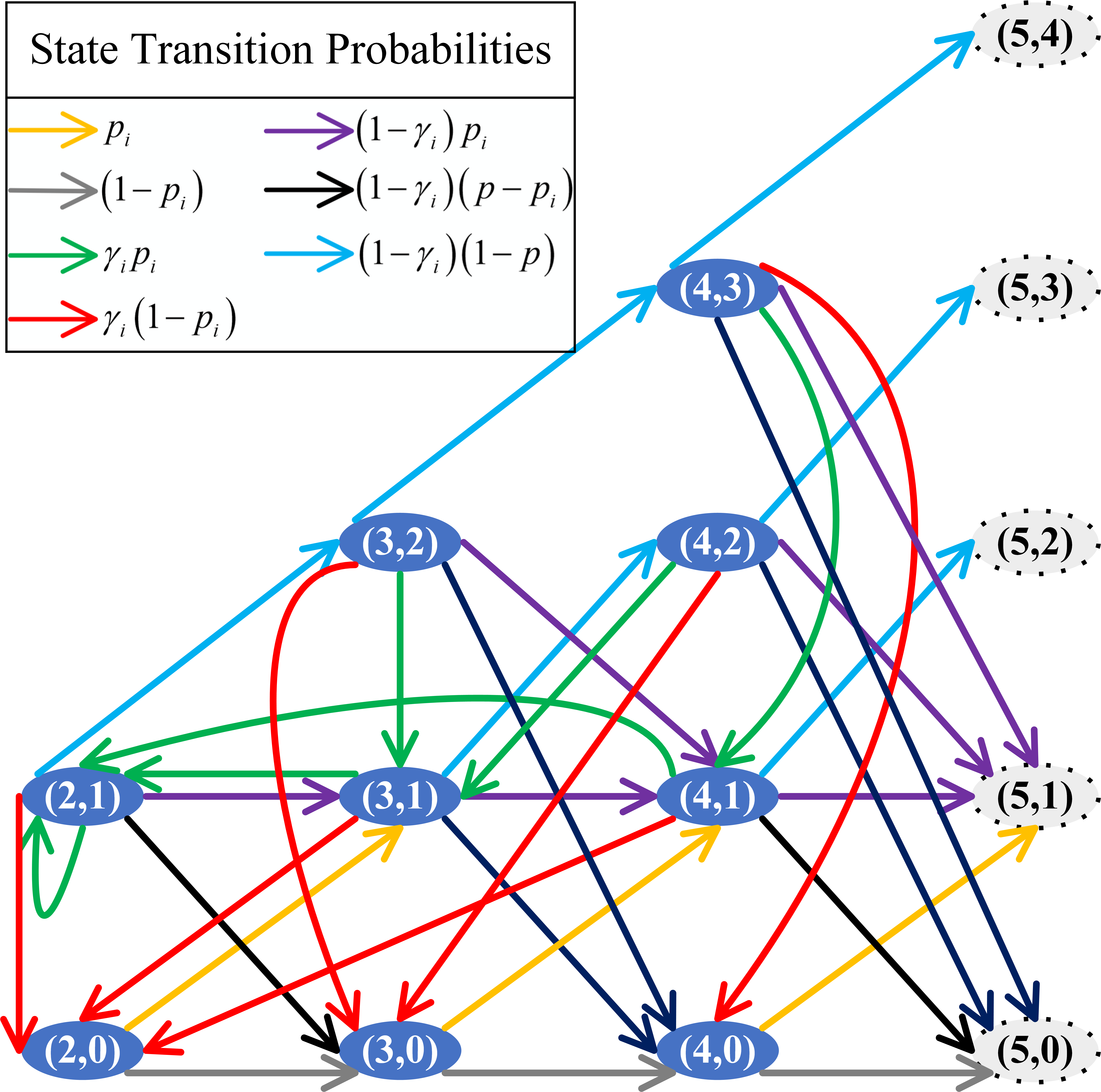
Figure 1: State transition diagram of the 2D age process. State transitions of states $(n,m)$ where $4\geq n>m\geq 0$ and $n\geq 2$, are shown as examples.

Based on the state transition analysis, it is found that the state of 2D age process at the next slot is only determined by the state at the current slot, regardless of the historical states. This indicates that $\bm{\Delta}_{i}(t)$ is a 2D DTMC. To be clarity, a schematic view of the state transitions are presented in Fig. 1.

III-C Stationary Equations of the 2D Age Process

Let us establish the stationary equations of 2D age process $\bm{\Delta}_{i}(t)$. Denote the stationary probabilities of $\bm{\Delta}_{i}(t)$ by $\pi^{(i)}_{(n,m)}$.

Note that all the states of $\bm{\Delta}_{i}(t)$ can be divided into five classes, i.e., $(2,1)$, $(2,0)$, $(n,1)$, $(n,0)$ and $(n,m)$, where $n>m\geq 2$. According to the state transitions (cf. Fig. 1) and the transition probabilities given by Eq.s (6), (7), (8), (9), (10), (11) and (12), it is found that: i) Only state $(n,1)$, $n\geq 2$, can transit to states $(2,1)$ and $(2,0)$ with probabilities $\gamma_{i}p_{i}$ and $\gamma_{i}(1-p_{i})$ respectively; ii) State $(n,1)$, $n\geq 3$, can be transited only from states $(n-1,0)$, $(k,n-1)$ for $k\geq n$, and $(n-1,k)$ for $n-1>k\geq 1$, with probabilities $p_{i}$, $\gamma_{i}p_{i}$ and $(1-\gamma_{i})p_{i}$ respectively; iii) State $(n,0)$, $n\geq 3$, can be transited only from states $(n-1,0)$, $(k,n-1)$ for $k\geq n$, and $(n-1,k)$ for $n-1>k\geq 1$, with probabilities $1-p_{i}$, $\gamma_{i}(1-p_{i})$ and $(1-\gamma_{i})(p-p_{i})$ respectively; iv) State $(n,m)$, $n>m\geq 2$, can be transited only from state $(n-1,m-1)$ with probability $\lambda_{i}:=(1-\gamma_{i})(1-p)$. Hence, the stationary equations of $\bm{\Delta}_{i}(t)$ can be formulated as

$$\pi^{(i)}_{(2,1)}= \gamma_{i}p_{i}\sum\nolimits_{n=2}^{\infty}\pi^{(i)}_{(n,1)},$$ (13a)

$$\pi^{(i)}_{(2,0)}= \gamma_{i}(1-p_{i})\sum\nolimits_{n=2}^{\infty}\pi^{(i)}_{(n,1)},$$ (13b)

$$\pi^{(i)}_{(n,1)}= p_{i}\pi^{(i)}_{(n-1,0)}+\gamma_{i}p_{i}\sum\nolimits_{k=n}^{\infty}\pi^{(i)}_{(k,n-1)}+(1-\gamma_{i})p_{i}\sum\nolimits_{k=1}^{n-2}\pi^{(i)}_{(n-1,k)},n\geq 3,$$ (13c)

$$\pi^{(i)}_{(n,0)}= (1-p_{i})\pi^{(i)}_{(n-1,0)}+\gamma_{i}(1-p_{i})\sum\nolimits_{k=n}^{\infty}\pi^{(i)}_{(k,n-1)}+(1-\gamma_{i})(p-p_{i})\sum\nolimits_{k=1}^{n-2}\pi^{(i)}_{(n-1,k)},n\geq 3,$$ (13d)

$$\pi^{(i)}_{(n,m)}= \lambda_{i}\pi^{(i)}_{(n-1,m-1)},n>m\geq 2.$$ (13e)

III-D Stationary Probabilities of the 2D Age Process as well as P.M.F. and Average of the Per-Source AoI

In this subsection, the stationary probabilities of the 2D age process $\bm{\Delta}_{i}(t)$ are found, based on which the p.m.f. and average of the per-source AoI ${\Delta}_{i}(t)$ are derived.

Based on the stationary equations of $\bm{\Delta}_{i}(t)$ formulated as Eq.s (13a)–(13e), the stationary probabilities can be obtained.

Lemma 1.

The stationary probabilities of the 2D age process $\bm{\Delta}_{i}(t)$ are given by

$$\pi^{(i)}_{(n,0)}= p_{i}\left({\frac{(\beta_{i}+\gamma_{i}-1)\beta^{n-1}_{i}-(\alpha_{i}+\gamma_{i}-1)\alpha^{n-1}_{i}}{\beta_{i}-\alpha_{i}}-\lambda^{n-1}_{i}}\right),n\geq 2,$$ (14)

$$\pi^{(i)}_{(n,m)}= \gamma_{i}p^{2}_{i}\lambda^{m-1}_{i}\left({\frac{\beta^{n-m}_{i}-\alpha^{n-m}_{i}}{\beta_{i}-\alpha_{i}}}\right),n>m\geq 1,$$ (15)

where $p_{i}$ is given by Eq. (4), $\lambda_{i}=(1-\gamma_{i})(1-p)$, as well as $\alpha_{i}$ and $\beta_{i}$ are the two different solutions of the quadratic equation $x^{2}-(1-\gamma_{i}p_{i}+\lambda_{i})x+\lambda_{i}=0$ w.r.t. $x$.

The proof of Lemma 1 is given in Appendix -A.

Note that the p.m.f. of the per-source AoI ${\Delta}_{i}(t)$ can be expressed by the stationary probabilities of $\bm{\Delta}_{i}(t)$, as

$$\pi_{i}(n)= \sum\nolimits_{m=0}^{n-1}\Pr\left\{\Delta_{i}=n,\Delta^{\prime}_{i}=m\right\}=\pi^{(i)}_{(n,0)}+\sum\nolimits_{m=1}^{n-1}\pi^{(i)}_{(n,m)},n\geq 2.$$ (16)

Based on Eq. (16) and Lemma 1, the p.m.f. and average of per-source AoI can be derived, as presented in the following.

Theorem 1.

The p.m.f. and average of the per-source AoI ${\Delta}_{i}(t)$ are respectively given by

$$\pi_{i}(n)= \gamma_{i}p_{i}\left({\frac{\beta^{n-1}_{i}-\alpha^{n-1}_{i}}{\beta_{i}-\alpha_{i}}}\right),n\geq 2,$$ (17)

$$\overline{\Delta}_{i}= \frac{\gamma_{i}+(1-\gamma_{i})p}{\gamma_{i}p_{i}}+1,$$ (18)

in which $p_{i}$ is given by Eq. (4), $p$ is given by Eq. (5), as well as $\alpha_{i}$ and $\beta_{i}$ are the two different solutions of the quadratic equation $x^{2}-(1-\gamma_{i}p_{i}+\lambda_{i})x+\lambda_{i}=0$ w.r.t. $x$.

Proof.

First, the p.m.f. of per-source AoI given by Eq. (17) can be obtained by substituting Eq.s (14) and (15) into Eq. (16) as well as using Eq. (31). On the other hand, one can obtain the average per-source AoI given by Eq. (18) by plugging Eq. (17) into Eq. (3) as well as utilizing $0<\alpha_{i}<1$, $0<\beta_{i}<1$, Eq. (31) and $\lambda_{i}=(1-\gamma_{i})(1-p)$. It is noteworthy that Eq. (31) as well as the proofs of $0<\alpha_{i}<1$ and $0<\beta_{i}<1$ are presented in Appendix -A. The detailed computations in this proof are omitted due to the page limit. ∎

By setting $q_{j}=0$, $j\in\mathcal{N}$, $j\neq i$, one can find that Theorem 1 is able to be applied to the single-source case, where the results in this work agree with those in [15].

IV Numerical Results

In this section, we first present and study the p.m.f. and average of per-source AoI. Simulations are provided to validate the theoretical analyses. Then, the effect of the retransmission protocol is analysed.

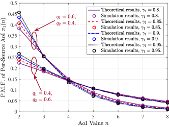
(a) The p.m.f. of per-source AoI.

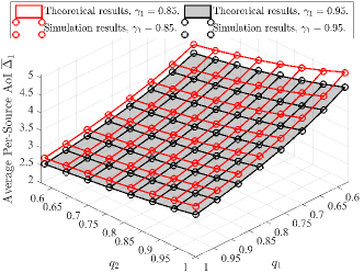
(b) The average per-source AoI.

Figure 2: The p.m.f. and average of per-source AoI in the two-source V2I link.

Fig. 2(a) presents the p.m.f. of per-source AoI versus transmission success probabilities. It is found that the probability distribution of per-source AoI tends to concentrate on the lower AoI value with the transmission success probability. This is consistent with the intuition that the better communication conditions leads to the better freshness. Fig. 2(b) describes the average per-source AoI versus update generation probabilities. It is shown that the average concerned-source AoI decreases with the update generation probability of the concerned source, however increases with that of the other source. Because: i) The increase of the concerned-source update generation probability raises the probability that the concerned-source update preempts the stale updates of all sources, which improves the concerned-source freshness; ii) Oppositely, the increases of the update generation probabilities of the other sources raise the probability that the concerned source is preempted by the other sources, which leads to the deterioration of the information freshness of concerned source. Besides, we simulate the per-source AoI processes in $10^{5}$ slots in Fig. 2. The simulation results verify the theoretical analyses.

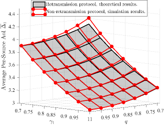
Figure 3: The average per-source AoIs in the two-source V2I links with and without the retransmission protocol.

Fig. 3 shows the average per-source AoIs in the V2I links with and without retransmission protocol. Consider two V2I links where one of them is adopted with the retransmission protocol (i.e., the V2I link considered before) while the other is not, and that the update generation probabilities in the V2I links are equal to $q$. In the latter V2I link, if an update transmission fails, this update is discarded. It is presented that the AoI in the V2I link with retransmission is lower especially when the update generation and transmission success probabilities are low, which represents that the retransmission can improve the information freshness. Because the retransmission enables the RI the chance to receive older but still fresh updates when no new update is generated at the vehicle. Moreover, it is found that the retransmission-leaded freshness improvement, i.e., the effect of the retransmission protocol increases along with the decreases of the update generation and transmission success probabilities. Because lower update generation and transmission success probabilities lead to higher probability of that the vehicle retransmits updates in the V2I link with retransmission while it is idle in the other V2I link.

V Conclusions

Information freshness of the V2I link, which is extracted as the multi-source Ber/Geo/1/1 preemptive queueing system with the heterogeneous service time, was studied in this work. To comprehensively characterize and evaluate the per-source AoI, we focused on the distribution and average. Specifically, to fully track the per-source AoI process, we introduced a Markov 2D age process. By analysing the state transitions, state transitions probabilities and establishing the stationary equations, we found the stationary probabilities of the 2D age process. Based on the stationary probabilities of the 2D age process, we derived the analytical expressions of the p.m.f. and average of the per-source AoI. Finally, the numerical results validated the correctness of the theoretical analyses.

-A Proof of Lemma 1

First, let us simplify the stationary equations of the 2D age process $\bm{\Delta}_{i}(t)$ given by Eq.s (13a)–(13e). Note that based on Eq.s (13a)–(13e), one can find the following results:

$$\pi^{(i)}_{(2,1)}= \frac{p_{i}}{1-p_{i}}\pi^{(i)}_{(2,0)},$$ (19)

$$\pi^{(i)}_{(n,m)}= \lambda^{m-1}_{i}\pi^{(i)}_{(n-m+1,1)},n>m\geq 1,$$ (20)

$$\sum\nolimits_{k=n}^{\infty}\pi^{(i)}_{(k,n-1)}= \sum\nolimits_{k=n}^{\infty}\lambda^{n-2}_{i}\pi^{(i)}_{(k-n+2,1)}=\lambda^{n-2}_{i}\sum\nolimits_{h=2}^{\infty}\pi^{(i)}_{(h,1)}=\frac{\lambda^{n-2}_{i}}{\gamma_{i}(1-p_{i})}\pi^{(i)}_{(2,0)},$$ (21)

$$\sum\nolimits_{k=1}^{n-2}\pi^{(i)}_{(n-1,k)}= \sum\nolimits_{k=1}^{n-2}\lambda^{k-1}_{i}\pi^{(i)}_{(n-k,1)}=\lambda^{n-2}_{i}\sum\nolimits_{r=2}^{n-1}\lambda^{-r+1}_{i}\pi^{(i)}_{(r,1)},n\geq 3.$$ (22)

Specifically, i) Eq. (19) holds following form Eq.s (13a) and (13b); ii) One can obtain Eq. (20) by repeatedly iterating Eq. (13e); iii) Eq. (21) holds following from Eq.s (13a) and (20); iv) Eq. (22) holds following from Eq. (20). By substituting Eq.s (19), (20), (21) and (22) into $\mathcal{E}_{1}$, the stationary equations of $\bm{\Delta}_{i}(t)$ can be simplified as

$$\pi^{(i)}_{(2,1)}= \gamma_{i}p_{i}\sum\nolimits_{n=2}^{\infty}\pi^{(i)}_{(n,1)},$$ (23a)

$$\pi^{(i)}_{(2,1)}= \frac{p_{i}}{1-p_{i}}\pi^{(i)}_{(2,0)},$$ (23b)

$$\pi^{(i)}_{(n,1)}= p_{i}\pi^{(i)}_{(n-1,0)}+\frac{p_{i}}{1-p_{i}}\lambda^{n-2}_{i}\pi^{(i)}_{(2,0)}+(1-\gamma_{i})p_{i}\lambda^{n-2}_{i}\sum\nolimits_{r=2}^{n-1}\lambda^{-r+1}_{i}\pi^{(i)}_{(r,1)},n\geq 3,$$ (23c)

$$\pi^{(i)}_{(n,0)}= (1-p_{i})\pi^{(i)}_{(n-1,0)}+\lambda^{n-2}_{i}\pi^{(i)}_{(2,0)}+(1-\gamma_{i})(p-p_{i})\lambda^{n-2}_{i}\sum\nolimits_{r=2}^{n-1}\lambda^{-r+1}_{i}\pi^{(i)}_{(r,1)},n\geq 3,$$ (23d)

$$\pi^{(i)}_{(n,m)}= \lambda^{m-1}_{i}\pi^{(i)}_{(n-m+1,1)},n>m\geq 1.$$ (23e)

Let us solve Eq.s (23a)–(23e). By observing, it is found that $\pi^{(i)}_{(n,0)}$ can be derived first. It is valuable to note that

$$\frac{1}{p_{i}}\left({\pi^{(i)}_{(n,1)}-p_{i}\pi^{(i)}_{(n-1,0)}-\frac{p_{i}}{1-p_{i}}\lambda^{n-2}_{i}\pi^{(i)}_{(2,0)}}\right)=\frac{1}{p-p_{i}}\left({\pi^{(i)}_{(n,0)}-(1-p_{i})\pi^{(i)}_{(n-1,0)}-\lambda^{n-2}_{i}\pi^{(i)}_{(2,0)}}\right),n\geq 3,$$ (24)

which holds following from Eq.s (23c) and (23d). One can deduce the relationship between $\pi^{(i)}_{(n,0)}$ and $\pi^{(i)}_{(n,1)}$, $n\geq 3$, as

$$\pi^{(i)}_{(n,1)}= \frac{p_{i}}{p-p_{i}}\left({\pi^{(i)}_{(n,0)}-(1-p)\pi^{(i)}_{(n-1,0)}-\frac{1-p}{1-p_{i}}\lambda^{n-2}_{i}\pi^{(i)}_{(2,0)}}\right),n\geq 3.$$ (25)

Based on Eq.s (23d) and (25), one can respectively obtain that

$$(1-\gamma_{i})(p-p_{i})\lambda^{n-3}_{i}\sum\nolimits_{r=2}^{n-2}\lambda^{-r+1}_{i}\pi^{(i)}_{(r,1)}= \pi^{(i)}_{(n-1,0)}-(1-p_{i})\pi^{(i)}_{(n-2,0)}-\lambda^{n-3}_{i}\pi^{(i)}_{(2,0)},n\geq 4,$$ (26)

$$\pi^{(i)}_{(n-1,1)}= \frac{p_{i}}{p-p_{i}}\left({\pi^{(i)}_{(n-1,0)}-(1-p)\pi^{(i)}_{(n-2,0)}-\frac{1-p}{1-p_{i}}\lambda^{n-3}_{i}\pi^{(i)}_{(2,0)}}\right),n\geq 4.$$ (27)

On the other hand, Eq. (23d) can be rewritten as

$$\pi^{(i)}_{(n,0)}\!=\!(1-p_{i})\pi^{(i)}_{(n-1,0)}\!+\!\lambda^{n-2}_{i}\pi^{(i)}_{(2,0)}\!+\!(1-\gamma_{i})(p-p_{i})\pi^{(i)}_{(n-1,1)}\!+\!\lambda_{i}(1-\gamma_{i})(p-p_{i})\lambda^{n-3}_{i}\sum\nolimits_{r=2}^{n-2}\lambda^{-r+1}_{i}\pi^{(i)}_{(r,1)},n\geq 3.$$ (28)

By substituting Eq.s (26) and (27) into Eq. (28) as well as utilizing $\lambda_{i}=(1-\gamma_{i})(1-p)$, the second-order recursive expression of $\pi^{(i)}_{(n,0)}$ can be deduced, as

$$\pi^{(i)}_{(n,0)}=(1-\gamma_{i}p_{i}+\lambda_{i})\pi^{(i)}_{(n-1,0)}-\lambda_{i}\pi^{(i)}_{(n-2,0)}-\frac{p_{i}}{1-p_{i}}\lambda^{n-2}_{i}\pi^{(i)}_{(2,0)},n\geq 4.$$ (29)

Let us derive $\pi^{(i)}_{(n,0)}$ by decreasing the order of the recursion. It is valuable to note that Eq. (29) can be rewritten as

$$\pi^{(i)}_{(n,0)}-\alpha_{i}\pi^{(i)}_{(n-1,0)}= \beta_{i}\left({\pi^{(i)}_{(n-1,0)}-\alpha_{i}\pi^{(i)}_{(n-2,0)}}\right)-\frac{p_{i}}{1-p_{i}}\lambda^{n-2}_{i}\pi^{(i)}_{(2,0)},n\geq 4,$$ (30)

in which $\alpha_{i}$ and $\beta_{i}$ satisfy that

$$\begin{cases}\alpha_{i}+\beta_{i}=1-\gamma_{i}p_{i}+\lambda_{i},\\ \alpha_{i}\beta_{i}=\lambda_{i},\end{cases}$$ (31)

i.e., $\alpha_{i}$ and $\beta_{i}$ are the two different solutions of the quadratic equation $x^{2}-(1-\gamma_{i}p_{i}+\lambda_{i})x+\lambda_{i}=0$ w.r.t. $x$. In fact, this quadratic equation always has two different solutions, since that the corresponding discriminant satisfies that

$$(1-\gamma_{i}p_{i}+\lambda_{i})^{2}-4\lambda_{i}=((1-\gamma_{i})+(1-p)+\gamma_{i}(p-p_{i}))^{2}-4(1-\gamma_{i})(1-p)> (-(1-\gamma_{i})+(1-p)+\gamma_{i}(p-p_{i}))^{2}$$

$$\geq 0,$$ (32)

where the first equality holds following from that $\lambda_{i}=(1-\gamma_{i})(1-p)$. By repeatedly iterating Eq. (30), one can obtain the first-order recursive expression of $\pi^{(i)}_{(n,0)}$, as

$$\pi^{(i)}_{(n,0)}-\alpha_{i}\pi^{(i)}_{(n-1,0)}=\beta^{n-3}_{i}\left({\pi^{(i)}_{(3,0)}-\alpha_{i}\pi^{(i)}_{(2,0)}}\right)-\frac{p_{i}}{1-p_{i}}\sum\nolimits_{k=0}^{n-4}{\beta^{k}_{i}\lambda^{n-k-2}_{i}}\pi^{(i)}_{(2,0)},n\geq 4.$$ (33)

Note that based on Eq. (23d) and $\lambda_{i}=(1-\gamma_{i})(1-p)$, $\pi^{(i)}_{(3,0)}$ can be expressed as

$$\pi^{(i)}_{(3,0)}=\left({\alpha_{i}+\beta_{i}-\frac{p_{i}\lambda_{i}}{1-p_{i}}}\right)\pi^{(i)}_{(2,0)}.$$ (34)

The first-order recursive expression can be simplified as

$$\pi^{(i)}_{(n,0)}=\alpha_{i}\pi^{(i)}_{(n-1,0)}+\left({\left({1+\frac{p_{i}\lambda_{i}}{(1-p_{i})(\lambda_{i}-\beta_{i})}}\right)\beta^{n-2}_{i}-\frac{p_{i}\lambda_{i}}{(1-p_{i})(\lambda_{i}-\beta_{i})}\lambda^{n-2}_{i}}\right)\pi^{(i)}_{(2,0)},n\geq 3.$$ (35)

By repeatedly iterating Eq. (35), $\pi^{(i)}_{(n,0)}$ can be determined by

$$\pi^{(i)}_{(n,0)}= \alpha^{n-2}_{i}\pi^{(i)}_{(n-1,0)}+\left({\left({1+\frac{p_{i}\lambda_{i}}{(1-p_{i})(\lambda_{i}-\beta_{i})}}\right)\sum\nolimits_{k=0}^{n-3}\alpha^{k}_{i}\beta^{n-k-2}_{i}-\frac{p_{i}\lambda_{i}}{(1-p_{i})(\lambda_{i}-\beta_{i})}\sum\nolimits_{k=0}^{n-3}\alpha^{k}_{i}\lambda^{n-k-2}_{i}}\right)\pi^{(i)}_{(2,0)}$$

$$= \frac{1}{\gamma_{i}(1-p_{i})}\left({\frac{(\beta_{i}+\gamma_{i}-1)\beta^{n-1}_{i}-(\alpha_{i}+\gamma_{i}-1)\alpha^{n-1}_{i}}{\beta_{i}-\alpha_{i}}-\lambda^{n-1}_{i}}\right){\pi^{(i)}_{(2,0)}},n\geq 2,$$ (36)

where the last equality holds following from Eq. (31). By substituting Eq. (36) into Eq. (25), as well as utilizing $\lambda_{i}=(1-\gamma_{i})(1-p)$ and Eq. (31), one can further obtain $\pi^{(i)}_{(n,1)}$, as

$$\pi^{(i)}_{(n,1)}=\frac{p_{i}}{1-p_{i}}\left({\frac{\beta^{n-1}_{i}-\alpha^{n-1}_{i}}{\beta_{i}-\alpha_{i}}}\right)\pi^{(i)}_{(2,0)},n\geq 2.$$ (37)

Furthermore, by plugging Eq. (37) into Eq. (23e), $\pi^{(i)}_{(n,m)}$, $n>m\geq 1$, can be determined by

$$\pi^{(i)}_{(n,m)}=\frac{p_{i}}{1-p_{i}}\lambda^{m-1}_{i}\left({\frac{\beta^{n-m}_{i}-\alpha^{n-m}_{i}}{\beta_{i}-\alpha_{i}}}\right)\pi^{(i)}_{(2,0)}.$$ (38)

Based on Eq.s (36) and (38), it is found that to obtain the explicit expressions of the stationary probabilities, $\pi^{(i)}_{(2,0)}$ needs to be derived first. In effect, according to the regularization condition of the stationary probabilities, one can obtain that

$$1=\sum\limits_{n>m\geq 0,n\geq 2}\pi^{(i)}_{(n,m)}=\sum\nolimits_{n=2}^{\infty}\left({\pi^{(i)}_{(n,0)}+\sum\nolimits_{m=1}^{n-1}\pi^{(i)}_{(n,m)}}\right)=\frac{\pi^{(i)}_{(2,0)}}{1-p_{i}}\sum\nolimits_{n=2}^{\infty}\frac{\beta^{n-1}_{i}-\alpha^{n-1}_{i}}{\beta_{i}-\alpha_{i}}=\frac{\pi^{(i)}_{(2,0)}}{\gamma_{i}p_{i}(1-p_{i})},$$ (39)

where the third equality holds following from Eq.s (31), (36) and (38), and the last equality holds based on that $0<\alpha_{i}<1$ and $0<\beta_{i}<1$ as well as Eq. (31). In particular, $0<\alpha_{i}<1$ and $0<\beta_{i}<1$ always hold since that

$$\alpha_{i}\beta_{i}= \lambda_{i}=(1-\gamma_{i})(1-p)>0,$$ (40)

$$0<\alpha_{i}+\beta_{i}= 1-\gamma_{i}p_{i}+\lambda_{i}<(1-\gamma_{i})(1-p)<1.$$ (41)

Eq. (39) implies that

$${\pi^{(i)}_{(2,0)}}={\gamma_{i}p_{i}(1-p_{i})}.$$ (42)

Finally, by plugging Eq. (42) into Eq.s (36) and (38), all the stationary probabilities of $\bm{\Delta}_{i}(t)$ can be given by Eq.s (14) and (15). The detailed computations in this proof are omitted.

References

- [1] K. Zheng et al., “Heterogeneous vehicular networking: A survey on architecture, challenges, and solutions,” IEEE Commun. Surv. Tut., vol. 17, no. 4, pp. 2377–2396, 2015.
- [2] X. Qin et al., “Distributed data collection in age-aware vehicular participatory sensing networks,” IEEE Internet of Things J., vol. 8, no. 19, pp. 14 501–14 513, 2021.
- [3] R. D. Yates et al., “Age of information: An introduction and survey,” IEEE J. Sel. Areas Commun., vol. 39, no. 5, pp. 1183–1210, 2021.
- [4] Z. Chen et al., “Improving the timeliness of two-source status update systems in Internet of vehicles with source-dedicated buffer: Resource allocation,” IEEE Trans. Veh. Technol., vol. 72, no. 7, pp. 9337–9350, 2023.
- [5] E. Najm et al., “Status updates through M/G/1/1 queues with HARQ,” in IEEE Int. Symp. Inf. Theory (ISIT), 2017, pp. 131–135.
- [6] E. Najm and E. Telatar, “Status updates in a multi-stream M/G/1/1 preemptive queue,” in IEEE Conf. Comput. Commun. Workshops (INFOCOM WKSHPS), 2018, pp. 124–129.
- [7] Z. Chen et al., “Age of information: The multi-stream M/G/1/1 non-preemptive system,” IEEE Trans. Commun., pp. 1–1, 2022.
- [8] V. Tripathi et al., “Age of information for discrete time queues,” 2019. [Online]. Available: arXiv:1901.10463
- [9] M. Moltafet et al., “Moment generating function of the AoI in a two-source system with packet management,” IEEE Wireless Commun. Lett., vol. 10, no. 4, pp. 882–886, 2021.
- [10] Y. Inoue et al., “A general formula for the stationary distribution of the age of information and its application to single-server queues,” IEEE Trans. Inf. Theory, vol. 65, no. 12, pp. 8305–8324, 2019.
- [11] M. Moltafet et al., “Moment generating function of age of information in multisource M/G/1/1 queueing systems,” IEEE Trans. Commun., vol. 70, no. 10, pp. 6503–6516, 2022.
- [12] T. Zhang et al., “AoI and PAoI in the IoT-based multi-source status update system: Violation probabilities and optimal arrival rate allocation,” IEEE Internet of Things J., pp. 1–1, 2023.
- [13] J. Zhang and Y. Xu, “On age of information for discrete time status updating system with infinite size,” in IEEE Inf. Theory Workshop (ITW), 2022, pp. 392–397.
- [14] ——, “On age of information for discrete time status updating system with Ber/G/1/1 queues,” in IEEE Inf. Theory Workshop (ITW), 2021, pp. 1–6.
- [15] A. Kosta et al., “The age of information in a discrete time queue: Stationary distribution and non-linear age mean analysis,” IEEE J. Sel. Areas Commun., vol. 39, no. 5, pp. 1352–1364, 2021.
- [16] N. Akar and O. Dogan, “Discrete-time queueing model of age of information with multiple information sources,” IEEE Internet of Things J., vol. 8, no. 19, pp. 14 531–14 542, 2021.