Exact Solutions of a Spin-Orbit Coupling Model in Two-Dimensional Central-Potentials and Quantum-Classical Correspondence

Abstract

In this paper we present both the classical and quantum periodic-orbits of a neutral spinning particle constrained in two-dimensional central-potentials with a cylindrically symmetric electric-field in addition which leads to an effective non-Abelian gauge field generated by the spin-orbit coupling. Coherent superposition of orbital angular-eigenfunctions obtained explicitly at the condition of zero-energy exhibits the quantum-classical correspondence in the meaning of exact coincidence between classical orbits and spatial patterns of quantum wave-functions, which as a consequence results in the fractional quantization of orbital angular-momentum by the requirement of the same rotational symmetry of quantum and classical orbits. A non-Abelian anyon-model emerges in a natural way.

1 Introduction

Quantum-classical correspondence (QCC) in one-dimensional space is a well known issue, for example, the quantum dynamics of harmonic oscillator in coherent states coincides exactly with the classical one. While it has attracted considerable interesting just recently for two-dimensional (2D) harmonic oscillator[1], central potentials [2, 3, 4] and for the non-Hermitian many-particle system, namely, a non-Hermitian N-particle Bose-Hubbard dimer with a complex on-site energy [5]. The QCC in stationary states, which means quite naturally and inevitably that quantum wave functions are localized on classical orbits, plays a central role in the explanation of many peculiar quantum-phenomena, for example, shell effects in nuclei and metallic clusters [6, 7], fluctuations of conductance in mesoscopic semiconductor billiards [8, 9], and the oscillations of photodetachment cross-sections [10, 11] as well.

In the interesting works[2, 3, 4, 12] both the classical and quantum periodic-orbits of a particle in 2D scalar-central-potentials of the general form are obtained analytically with the zero total-energy and it is shown that the fractional angular-momentum-quantization can be determined by the QCC with the wave functions well localized on the classical periodic-orbits, which imposes a special boundary condition on the angular wave functions [3, 4, 12]. The zero-energy states are of importance for the description of cold-atom collisions [13, 14] and some vortex lattices [15]. The spin coherent states [16, 17, 18, 19] which are the most representative states related to classical dynamics and the most persistent states describing the interaction with the environment[20] are essential in the construction of quantum wave functions localized on the classical orbits in 2D central-potentials and the 2D harmonic oscillators[1] as well.

The spin-orbit (SO) interaction, which coupling the internal and orbital degrees of freedom exists intrinsically in semiconductors, is responsible for the quantum spin-Hall-effect[21, 22] and has been realized experimentally for pseudo spin-1/2 atomic-condensates recently [23, 24, 25]. It has become a very active field of research known as spintronics[26], where the spin degree of freedom of the electron is exploited for improved functionality of electronic devices. Moreover, the SO is crucial in the description of tunneling magnetoresistance [27] and also of cold atom-dynamics[28]. SO coupling is naturally depicted as the interaction between an effective non-Abelian gauge potential and a particle with spin. In quantum systems, the concept of non-Abelian gauge-field was proposed by Wilczek and Zee in the context of Berry phase for a system of degenerate ground-states [29]. The realization of non-Abelian gauge fields in cold atomic systems was theoretically suggested for a neutral spinning particle (pseudo-spin) in electromagnetic fields [30] as well as in a cavity QED system [31].

As of yet the QCC in the meaning that the density of wave functions is well localized on the classical orbits has been studied only for the point particle without spin, since the spin is directly introduced in non-relativistic quantum mechanics and has no classical counterpart. The dynamics for a particle with intrinsic angular momentum or spin is different from that of a point particle and the key point is the definition of classical spin-variable [32], based on which the both classical and quantum dynamics of a neutral spinning-particle in the Aharonov-Casher (AC) gauge field[33] was explored long ago [34] giving rise to the theoretical analyses of neutron-experiments for the Aharonov-Bohm effect [35]. We in the present paper study the QCC for a spinning particle confined in 2D central-potentials, in which macroscopic wave functions are constructed by the coherent superposition of orbital angular-eigenfunctions in the spirit of usual SU(2) spin coherent-states [16, 17, 18, 19]. Both classical orbits and quantum probability-clouds in the macroscopic states are obtained, which possess the exactly same spatial patterns. Moreover, it is shown that the SO coupling leads naturally to a non-Abelian gauge potential and acts as a non-Abelian anyon model, which may be realized with cold-atoms in planner traps or with planner quantum-dots.

The classical dynamics of spinning particle with spin treated as a classical variables is formulated and general solutions of periodic-orbits are obtained in Sec. II. In Sec. III, the QCC is established by the coherent superposition of orbital angular-eigenfunctions, which along with the radial-part solutions of the Schr$\ddot{o}$dinger equation form the desired probability clouds of wave functions well localized on classical periodic orbits. In addition both the classical and quantum precessions of spin variables are also demonstrated explicitly. Our solutions give rise to the explicit non-Abelian gauge potential and the property of non-Abelian anyon.

2 Classical dynamics of spin and periodic orbits

2.1 Lagrangian and Hamiltonian

The classical dynamics of a neutral spinning-particle constrained in the 2D central-potential of $V(r)=-\frac{\varrho}{r^{2k+2}}$, with ${r}=\sqrt{x^{2}+y^{2}}$ and $\varrho$ being a potential constant, can be described by the Lagrangian

$$\mathcal{L}_{0}=\frac{1}{2}[M\mathbf{\dot{r}}^{2}+i\lambda Tr(\sigma_{3}g^{-1}\dot{g})]-V(r)$$ (1)

where $M$ and $\lambda$ are mass and spin-value of the particle. The configuration space is a product space $\mathbb{R}^{2}\times\Gamma$, where $\Gamma=\{g\}$ denotes the usual spin-$\frac{1}{2}$ representation of the rotation group with element $g$ being a $SU(2)$ matrix [32, 35], $g^{\dagger}g=1,\det g=1.$ The (classic) dynamic variables of spin $\mathbf{S}$ constrained by $\mathbf{S}^{2}=S_{1}^{2}+S_{2}^{2}+S_{3}^{2}=\lambda^{2}$ are connected with the group element $g$ through the relation

$$\mathbf{S\cdot\mbox{\boldmath$\sigma$}}=\lambda g\sigma_{3}g^{-1}$$ (2)

where $\sigma_{i}$ is Pauli matrices. We moreover assume that a cylindrically symmetric electric field

$$\mathbf{E=}\frac{\eta\mathbf{e}_{\mathbf{r}}}{r}$$ (3)

is applied, which can be realized by an infinitely long line-charge with charge-density (the charge of per unit length) $\eta$. The interaction part of Lagrangian between the moving spin of velocity $\mathbf{\dot{r}}$ and the electric field, i.e. the SO, is

$$\mathcal{L}_{i}=\frac{\mu\lambda}{2c}Tr[g\sigma_{3}g^{-1}(\mathbf{E\times\mathbf{\dot{r}}})\cdot\mathbf{\mbox{\boldmath$\sigma$}}]$$ (4)

where $\mu$ denotes the magnetic moment of spinning particle. Using relation Eq. (2), the total Lagrangian including the SO coupling Eq. (4) $\mathcal{L}=\mathcal{L}_{0}+\mathcal{L}_{i}$can be written as familiar form,

$$\mathcal{L}=\mathcal{L}_{0}+\frac{\mu}{c}[\mathbf{\dot{r}\cdot(S\times E)}]$$ (5)

Noticing that the spin variable $\mathbf{S}$ is a function of $g$, we can obtain equations of motion in the configuration space by means of the variation $\delta\int\mathcal{L}dt=0$ with respect to space coordinates $\mathbf{r}$ and spin-space coordinate $g$ respectively

$$M\mathbf{\ddot{r}+\dot{p}}_{i} = -\nabla V(r)+\frac{\mu}{c}\nabla[\mathbf{S\cdot}(\mathbf{E\times\dot{r}})]$$ (6)

$$\mathbf{\dot{S}} = \frac{\mu}{c}(\mathbf{\dot{r}\times E})\times\mathbf{S}$$ (7)

where

$$\mathbf{p}_{i}=\frac{\mu}{c}\mathbf{(S\times E)}$$

is called the intrinsic momentum[35]. In the absence of SO coupling (i.e. $\mathbf{E=0}$), the spin variables become a conserved quantity and the equation of motion Eq. (6) reduces to that of a point particle in the central potential $V(r)$. The canonical momentum is defined by

$$\mathbf{p=}\nabla_{\mathbf{\dot{r}}}\mathcal{L}=M\mathbf{\dot{r}+}\frac{\mu}{c}\mathbf{(S\times E)}$$ (8)

Then the Hamiltonian has the usual minimum coupling form

$$H=\frac{[\mathbf{p-\frac{\mu}{c}A}]^{2}}{2M}\mathbf{+}V(r)$$ (9)

with an effective vector gauge-potential $\mathbf{A=S\times E}$, which, we will see, becomes a pseudo non-Abelian gauge field after quantization. The gauge field structure may be the most significant consequence of our formalism for the introduction of classical spin-variables.

2.2 Reduced classical equation of motion

The coupled classical equations of motion (6) and (7) can be reduced (in the initial condition $\dot{z}|_{t=0}=0$) to[34, 35]

$$M\ddot{x} =-\frac{\partial}{\partial x}V(r)$$

$$M\ddot{y} =-\frac{\partial}{\partial y}V(r)$$ (10)

and

$$\dot{S}_{x} = -\frac{q}{r^{2}}[\dot{x}y-\dot{y}x]S_{y}$$

$$\dot{S}_{y} = \frac{q}{r^{2}}[\dot{x}y-\dot{y}x]S_{x}$$

$$\dot{S}_{z} = 0$$ (11)

up to the order $0$($q^{2}$), where $q=\eta\mu/c<<1$ is a dimensionless small parameter, since the SO coupling is an effect of relativity. It is interesting to see that the motion of central mass is effectively confined in a 2D plane and is not affected by the spin motion. The solutions of intrinsic (spin variables) motions are found as

$$S_{x}(t) = S_{x}(0)\cos[q\varphi(t)]+S_{y}(0)\sin[q\varphi(t)]$$

$$S_{y}(t) = -S_{x}(0)\sin[q\varphi(t)]+S_{y}(0)\cos[q\varphi(t)]$$

$$S_{z}(t) = S_{z}(0)$$ (12)

where $\varphi(t)=\arctan y(t)/x(t)$ and $S_{i}(0)(i=x,y,z)$ denotes the initial value of spin variables. The motion of spin variables is nothing but a Larmor precession around the $z$-axis with the $z$-component being constant ( $S_{z}$=const). The precession angle $q\varphi(t)$ is proportional to the polar angle of particle position $\varphi(t)$. For the case of non-integer $q$ the spin vector does not return to its original orientation even if the particle comes full circle. This , we will see, is the dynamic reason of the non-Abelian anyon. The motion of central mass along $z$-direction is a relativistic oscillating-perturbation around the $z=0$ plane with velocity

$$\dot{z}=-\frac{q}{Mr}[S_{x}(0)\sin\varphi-S_{y}(0)\cos\varphi]$$

which does not affect the planner motion of Eq. (10) and the spin precession of Eq. (11) for periodic orbits in the central potential. Thus we can consider only the motion of central mass in 2D space with spin-orbit coupling.

2.3 Effective Hamiltonian in 2D spatial space and classical orbits

The effective Lagrangian corresponding to the reduced equations of motion Eq. (10-11) in 2D spatial space of polar coordinate is seen to be $\mathcal{L}^{e}=\mathcal{L}_{0}^{e}+\mathcal{L}_{i}^{e}$ with $\mathcal{L}_{0}^{e}=\frac{M}{2}(\dot{r}^{2}+r^{2}\dot{\varphi}^{2})-V(r)$, where the SO coupling term is of the Wess-Zummino type,

$$\mathcal{L}_{i}^{e}=qS_{z}\dot{\varphi}$$ (13)

The canonical momentums conjugate to $r,\varphi$ are

$$p_{r} =\frac{\partial\mathcal{L}^{e}}{\partial\dot{r}}=M\dot{r}$$ (14)

$$L_{z}^{c} =L_{z}^{K}+qS_{z}$$ (15)

$L_{z}^{c}$ is the canonical angular momentum (CAM), while $L_{z}^{K}$ $=Mr^{2}\dot{\varphi}$ is kinetic angular momentum (KAM). The Hamiltonian is

$$H=\frac{p_{r}^{2}}{2M}+\frac{1}{2Mr^{2}}[L_{z}^{c}-qS_{z}]^{2}+V(r)$$ (16)

Considering non-zero initial KAM of the value

$$L_{z}^{K}=\gamma\hbar$$ (17)

the orbital motion of zero-energy satisfies the equation

$$\frac{(L_{z}^{K})^{2}}{2Mr^{4}}[(\frac{dr}{d\varphi})^{2}+r^{2}]-\frac{\varrho}{r^{2k+2}}=0$$ (18)

Changing variables successively to $\xi=r/a_{c},y=\xi^{k}$ and $x=\cos^{-1}y$, a direct mathematical solution[2] can be obtained by integrating the orbital Eq. (18)

$$\varphi-\varphi_{0} =\int_{1}^{\xi}\frac{\xi^{k-1}}{\sqrt{1-\xi^{2k}}}d\xi=k^{-1}\int_{1}^{y}\frac{dy}{\sqrt{1-y^{2}}}$$

$$=-k^{-1}\int_{0}^{\arccos y}dx$$

and the result is

$$\xi^{k}=\cos k(\varphi-\varphi_{0})$$

or

$$r^{k}=a_{c}^{k}\cos[k(\varphi-\varphi_{0})]$$ (19)

where $a_{c}^{2k}={2M\varrho/(L_{z}^{K})^{2}}={2M\varrho}/{\gamma^{2}\hbar^{2}}$. The classical orbits with the initial angle setting to zero ($\varphi_{0}=0$ ) are shown in Fig. 1 for the closed orbits with the scalar potentials of power-indexes $k=1,7/3,4,9/2,5$, $17/3$, and in Fig. 2 for the open orbits with potential power-indexes $k=$ $-6$ ,$-17/4$, where we set the dimensionless constant $2M\varrho/\hbar^{2}=1$ in the numerical calculation. The classical orbits Eq. (19) are invariant under a rotation-angle $2\pi/\left|k\right|$ and the $2\pi$-symmetry holds only for $k=1$. The initial values of KAM for closed orbits in Fig. 1 are set by $\gamma=15,35,60,135/2,85,75,$ respectively, while $\gamma$= $255/4$, $90$ in Fig. 2.

3
Quantum wave functions and QCC

3.1 Pseudo non-Abelian gauge field

After quantization the gauge field in Hamiltonian Eq. (9) becomes a field-valued operator $\mathbf{A=S\times E}$, with

$$\mathbf{S=\hbar}\frac{\mbox{\boldmath$\sigma$}}{2}$$ (20)

for the spin-1/2 case, which is a matrix field called  pseudo non-Abelian gauge field. The Hamilton operator in the representation of a covariant derivative can be written as

$$H=-\frac{\hbar^{2}}{2M}\sum_{i=x,y,z}D_{i}^{2}\mathbf{+}V(r)$$ (21)

where

$$D_{i}=\frac{\partial}{\partial x_{i}}-i\beta A_{i}$$ (22)

denotes a covariant derivative with $\beta=\frac{\mu}{2c}$. The non-Abelian gauge field

$$A_{i}=\sum_{j,k=x,y,z}\epsilon_{ijk}\sigma_{j}E_{k}$$ (23)

(where $\epsilon_{ijk}$ is the Levi-Civita tensor) has the explicit form

$$A_{x} = -\frac{\eta\sin\varphi}{r}\sigma_{z}$$

$$A_{y} = \frac{\eta\cos\varphi}{r}\sigma_{z}$$

$$A_{z} = \frac{\eta}{r}(\sin\varphi\sigma_{x}+\cos\varphi\sigma_{y})$$ (24)

for the cylindrically symmetric electric field Eq. (3). The effective magnetic-field can be expressed by the antisymmetric tensor

$$F_{i,j}=\frac{i}{\beta}[D_{i},D_{j}]=(\frac{\partial A_{j}}{\partial x_{i}}-\frac{\partial A_{i}}{\partial x_{j}})-i\beta[A_{i},A_{j}]$$ (25)

which gives rise to

$$B_{x} = 0$$

$$B_{y} = \frac{\eta}{r^{2}}\{(1-\beta\eta)\sin 2\varphi\sigma_{x}+[(1-\beta\eta)\cos 2\varphi+\beta\eta]\sigma_{y}\}$$

$$B_{z} = \frac{\eta}{r^{2}}\{[(1-\beta\eta)\cos 2\varphi-\beta\eta]\sigma_{x}-(1-\beta\eta)\sin 2\varphi\sigma_{y}\}$$ (26)

The unitary operator of gauge transformation is defined as

$$U=e^{i\beta\sum_{i}f_{i}\sigma_{i}}$$ (27)

where $f$ is a function of space coordinate. The covariant derivative operator under the gauge transformation becomes

$$D_{i}^{{}^{\prime}}=UD_{i}U^{{\dagger}}=\frac{\partial}{\partial x_{i}}-i\beta A_{i}^{{}^{\prime}}$$

where gauge field becomes

$$A_{i}^{{}^{\prime}}=UA_{i}U^{{\dagger}}-\frac{i}{\beta}(\frac{\partial U}{\partial x_{i}})U^{{\dagger}}$$

Spinor wave function transformation is

$$\psi^{{}^{\prime}}=U\psi$$ (28)

It is worth while to remark that the non-Abelian gauge field in quantum mechanics is only of formal meaning which is a concept first introduced by Wilczek and Zee[29]. To avoid confusion we call it the pseudo non-Abelian gauge field. The SO coupling and non-Abelian gauge field have become an active research field of ultracold atoms in optical fields. The gauge field method might help us to have a deeper understanding of the fundamental quantum phenomena in the atomic, molecular and optical physics.

3.2 2D wave functions, fractional angular momentum and QCC

We are particularly interested in the QCC. To this end we turn to the quantum mechanics of reduced 2D problem with Hamiltonian Eq. (16). In the polar coordinate, the stationary Schrödinger equation of zero-energy with wave function $\Psi=R(r)Y_{j,\chi}(\varphi)$

$$\frac{-\hbar^{2}}{2M}\{\frac{\partial^{2}}{\partial r^{2}}+\frac{1}{r}\frac{\partial}{\partial r}+\frac{1}{r^{2}}[\frac{\partial}{\partial\varphi}-i\frac{1}{2}q\hat{\sigma}_{z}]^{2}\}\Psi+V(r)\Psi=0$$

becomes

$$(\frac{\partial^{2}}{\partial r^{2}}+\frac{1}{r}\frac{\partial}{\partial r}-\frac{j^{2}}{r^{2}})R_{j}(r)+\frac{2M}{\hbar^{2}}\frac{\varrho}{r^{2k+2}}R_{j}(r) = 0$$ (29)

$$(\frac{\partial}{\partial\varphi}-i\frac{1}{2}q\hat{\sigma}_{z})^{2}Y_{j,\chi}(\varphi) = -j^{2}Y_{j,\chi}(\varphi)$$ (30)

where $\chi$ denotes the spin index and $j$ is the eigenvalue of orbital angular-momentum. The angular wave function, which possesses a non-Abelian topological phase, is seen to be

$$Y_{j,\chi}(\varphi)=Y_{j}(\varphi)e^{i(q\hat{\sigma}_{z}/2)\varphi}|\chi\rangle$$ (31)

with $Y_{j}(\varphi)=C_{j}e^{ij\varphi}$ where $C_{j}=\sqrt{\left|k\right|/2\pi}$ is the normalization constant depending on the angular momentum quantization in 2D spatial space and $|\chi\rangle$ denotes a spin state. We consider the QCC with the meaning that both the probability density of wave functions and the expectation value of spin-operator well coincide with the classical orbits Eq. (19) and the classical spin precession Eq. (12) respectively. This kind of QCC results in a special boundary condition of the angular eigenstates such that the rotational period of angular wave-functions, which is not necessarily 2$\pi$, should be the same as that of classical orbits i.e. $Y_{j}(\varphi)=Y_{j}(\varphi+\frac{2\pi}{\left|k\right|})$. Thus the CAM eigenvalue is no longer integer but should be set as

$$j=\nu\left|k\right|$$ (32)

where $\nu$ is a non-vanishing integer. Introducing the dimensionless radius $z={\tilde{a}_{q}}/{r}$ and a parameter $\tilde{a}_{q}$ with dimension of length the radius equation,

$$\ (\frac{\partial^{2}}{\partial r^{2}}+\frac{1}{r}\frac{\partial}{\partial r}-\frac{j^{2}}{r^{2}})R_{j}(r)+\frac{2M}{\hbar^{2}}\frac{\varrho}{r^{2k+2}}R_{j}(r)=0$$

becomes

$$[z^{2}\frac{d^{2}}{dz^{2}}+z\frac{d}{dz}+B^{2}z^{2k}-j^{2}]\Theta_{j}(z)=0$$

where $B^{2}={2M\varrho}/{\hbar^{2}\tilde{a}_{q}^{2k}}$, and can be rewritten as

$$\{y^{2}\frac{d^{2}}{dy^{2}}+y\frac{d}{dy}+[y^{2}-\nu^{2}]\}\Theta_{j}(y)=0$$ (33)

by the change of variables $\xi=z^{k}$ and $y={B}\xi/{k}$. The solution is Bessel function of order $\nu$,

$$\ \Theta_{j}(y)=N_{j}J_{\nu}(y)$$

which is the same as in Ref. [3]. The radius wave function is

$$R_{j}(r)=N_{j}J_{\nu}(\frac{1}{\left|k\right|r^{k}})$$

With the angular quantum-number $j=\nu\left|k\right|$, classical orbits can be mimicked by the probability density of wave functions, which we will see in the followings. The normalization constant obtained from the integral

$$\ \int_{0}^{\infty}R_{j}^{2}(r)rdr=1$$

with the infinite integrals of Bessel function[36] is

$$\left|N_{j}\right|^{2}=2\sqrt{\pi}\left|{k}\right|^{\frac{2}{k}+1}\frac{\Gamma(\frac{1}{k}+1)\Gamma(\frac{1}{k}+\nu+1)}{\Gamma(\frac{1}{k}+\frac{1}{2})\Gamma(\nu-\frac{1}{k})}$$ (34)

by setting $B\tilde{a}_{q}^{k}=1$. It is of fundamental importance to show the correspondence between wave function and classical orbit. Recently, it was demonstrated that the probability density of wave function can be well localized on the classical orbits in a 2D central potentials with the representation of $SU(2)$ coherent states[3, 4], which is a superposition of degenerate eigenstates. To coincide with the classical orbits we construct the macroscopic wave functions in the spirit of $SU(2)$ coherent-state representation in terms of the degenerate partial-waves and the macroscopic wave-function is

$$\Psi_{n}=\frac{1}{2^{n/2}}\sum_{\nu=0}^{n}{n\choose\nu}^{1/2}R_{j}(r)Y_{j,\chi}(\varphi)$$ (35)

which is normalized to unity in the angular range of $\varphi$ being from $-\pi/\left|k\right|$ to $\pi/\left|k\right|$. The probability densities $\Psi_{n}^{{\dagger}}\Psi_{n}$ of macroscopic state with $n=30$ shown in Figs. 3 and 4 are in excellent agreement with the classical orbits (see Figs.1,2) indicating the exact QCC. As a consequence we have the fractional orbital-angular-momentum with the eigenvalue $j=\nu\left|k\right|$, if $\nu\left|k\right|$ is a fractional number.

Besides the spatial orbits the QCC holds also for the spin motion. To this end we begin with the expectation value of Heisenberg equation of the spin operator in the macroscopic wave function Eq. (35), which gives rise to

$$\langle\dot{\sigma}_{x}\rangle = q\dot{\varphi\langle}\sigma_{y}\rangle$$

$$\langle\dot{\sigma}_{y}\rangle = -q\dot{\varphi\langle}\sigma_{x}\rangle$$

$$\langle\dot{\sigma}_{z}\rangle = 0$$

where

$$\ \langle\sigma_{i}\rangle=\langle\chi|\sigma_{i}|\chi\rangle$$

and the constant being angular velocity is calculated as

$$\ \dot{\varphi}=\langle\psi_{n}|\frac{\hat{L}_{z}^{K}}{Mr^{2}}|\psi_{n}\rangle$$

in which $\psi_{n}=\frac{1}{2^{n/2}}\sum_{\nu=0}^{n}{n\choose\nu}^{1/2}R_{j}(r)Y_{j}(\varphi)$ is the macroscopic orbital-wave-function and $\hat{L}_{z}^{K}$ is the orbital angular momentum operator. The expectation value of spin equation of motion in the macroscopic state is the same as the classical one Eq. (11).

3.3 Non-Abelian Anyon

The orbital angular momentum operator is $\hat{L}_{z}^{K}=-i\hbar\partial/\partial\varphi$ and total angular-momentum operator i.e the CAM operator reads

$$\hat{L}_{z}^{c}=-i\hbar\frac{\partial}{\partial\varphi}+\frac{1}{2}q\hbar\hat{\sigma}_{z}$$ (36)

which possesses eigenstates $Y_{j,\chi}(\varphi)$ if the spin state is chosen as eigenstates of $\hat{\sigma}_{z}$, such that $|\chi\rangle=|\pm\rangle$, where $\hat{\sigma}_{z}|\pm\rangle=\pm|\pm\rangle$. Thus the total angular-momentum spectrum $\Lambda$ is seen to be

$$\Lambda=(\nu\left|k\right|\pm\frac{1}{2}q)\hbar$$ (37)

with $\nu$ being a integer. The angular momentum is quantized with an eigenvalue-space $\left|k\right|$, which can be a fractional number determined completely by the QCC. The gauge potential of SO coupling can shift the spectrum of CAM by an arbitrary value $q\hbar/{2}$, which results in a common topological phase for all wave functions in the given model, since $q$ is not necessarily an integer. Thus non-Abelian anyons[37] naturally appear, which obey non-Abelian braiding statistics.

4 Conclusion

In summary, both classical and quantum periodic orbits of a SO coupling model in a wide class of central potentials are obtained analytically, where the classical spin-variables are introduced in a consistent way to give rise to the correct equation of motion. The exact QCC with a perfect match between classical orbits and the spatial probability clouds is found with the coherent superposition of angular wave functions, which imposes a special boundary condition on the angular wave functions resulting in the fractional angular momentum quantization. Simultaneously, the QCC for the spin degree of freedom is also established, which displays the exactly same spin-precession in addition to the orbital motion of central mass. The SO coupling model exhibits explicitly a pseudo non-Abelian gauge field and the anyon behavior.

Figure 1: Closed classical periodic-orbits for various value of KAM with potential power-indexes $k=1,7/3,4,9/2,17/3,5$.

Figure 2: Open classical periodic orbits for various value of KAM with the potential power-indexes $k=-6,-17/4$.

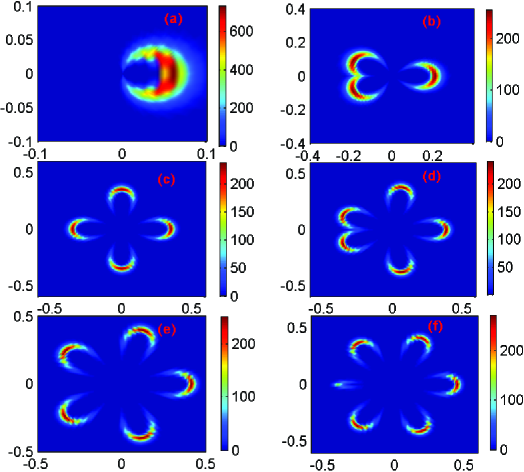
Figure 3: (color online) Probability density $\left|Y_{j,\chi}(\varphi)\right|^{2}$ for the parameters corresponding to closed classical orbits shown in Fig. 1.

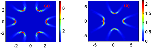
Figure 4: (color online) Probability density $\left|Y_{j,\chi}(\varphi)\right|^{2}$ for the parameters corresponding to open classical orbits shown in Fig. 2.

References

- [1] Y. F. Chen, Phys. Rev. A. 83 (2011) 032124.
-
[2]
M. M. Nieto and J. Daboul, Phys. Rev. E. 52 (1995) 4430.
J. Daboul and M. M. Nieto, Int. J. Mod. Phys. A. 11 (1996) 3801. - [3] A. J. Makowski and K. J. Gorska, J. Phys. A: Math. Theor. 40 (2007) 11373.
- [4] A. J. Makowski and K. J. Gorska, Phys. Rev. A. 79 (2009) 052116.
- [5] E. M. Graefe, H. J. Korsch and A. E. Niederle, Phys. Rev. A. 82 (2010) 013629.
- [6] M. Brack, Rev. Mod. Phys. 65 (1993) 677.
- [7] W. A. De Heer, Rev. Mod. Phys. 65 (1993) 611.
- [8] I. V. Zozoulenko and K. F. Berggren, Phys. Rev. B. 56 (1997) 6931.
- [9] R. Brunner, R. Meisels, F. Kuchar, R. Akis, D. K. Ferry and J. P. Bird, Phys. Rev. Lett. 98 (2007) 204101.
- [10] A. D. Peters, C. Jaffé and J. B. Delos, Phys. Revs. Lett. 73 (1994) 2825.
- [11] C. Bracher and J. B. Delos, Phys. Rev. Lett. 96 (2006) 100404.
- [12] A. J. Makowski, Ann. Phys. 325 (2010) 1622.
- [13] H. R. Sadeghpour, J. L. Bohn, M. J. Cavagnero, B. D. Esry, I. I. Fabrikant, J. H. Macek and A. R. P. Rau, J. Phys. B: At. Mol. Opt. Phys. 33 R (2000) 93.
- [14] H. Wang, X. T. Wang, P. L. Gould and W. C. Stwalley, Phys. Rev. Lett. 78 (1997) 4173.
- [15] T. Kobayashi, Physica A. 303 (2002) 469.
- [16] E. Schrödinger, Naturwissenschaften. 14 (1926) 664.
- [17] W. M. Zhang, D. H. Feng and R. Gilmore, Rev. Mod. Phys. 62 (1990) 867.
- [18] J. R. Klauder and Bo. Sture. Skagerstam, Coherehent States Applications in Physics and Mathematical Physics. (World Scientific, Singapore, 1985).
- [19] Kh. Muminov and Y. Yousefi, arXiv:1103.6080 (2011).
- [20] W. H. Zurek, S. Habib and J. P. Paz, Phys. Rev. Lett. 70 (1993) 1187.
-
[21]
S. Murakami et al., Science. 301 (2003) 1348.
J. Sinova et al., Phys. Rev. Lett. 92 (2004) 126603. -
[22]
Y. K. Kato et al., Science. 306 (2004) 1910.
J. Wunderlich et al., Phys. Rev. Lett. 94 (2005) 047204. - [23] T. L. Ho and S. Z. Zhang, arXiv: 1007.0650(2010).
- [24] Y. J. Lin, K. Jiménez. García and I. B. Spielman, Nature. 471 (2011) 83.
- [25] S. K. Yip, arXiv:1008.2263 (2010).
- [26] S. A. Wolf et al., Science. 294 (2001) 1488.
- [27] A. Matos. Abiague and J. Fabian, Phys. Rev. B. 79 (2009) 155303.
- [28] A. Jacob, P. Öhberg and G. Juzeliūnas, L. Santos, Appl. Phys. B. 89 (2007) 439.
- [29] F. Wilczek and A. Zee, Phys. Rev. Lett. 52 (1984) 2111.
-
[30]
R. Dum and M. Olshanii, Phys. Rev. Lett. 76 (1996) 1788.
Y. J. Lin et al., Phys. Rev. Lett. 102 (2009)130401. - [31] J. Larson and S. Levin, Phys. Rev. Lett. 103 (2009) 013602.
- [32] A. P. Balachandran, G. Marmo, B.S. Skagerstam and A. Stern, Gauge Symmetries and Fibre Bundels. (Springer Verlag, berlin, 1983).
- [33] Y. Aharonov and A. Casher, Phys. Rev. Lett. 53 (1984) 319.
- [34] J. Q. Liang and X. X. Ding, Phys. Lett. A. 176 (1993) 165.
- [35] J. Q. Liang, G. Marmo, A. Simoni and F. Zaccaria, Mod. Phys. Lett. A. 5 (1990) 2361.
- [36] G. N. Watson, Theory of Bessel Function. (Cambrige Univ.Press, London, 1952).
-
[37]
F. Wliczek, Phys. Rev. Lett. 48 (1982) 1144.
F. Wliczek, Phys. Rev. Lett. 49 (1982) 957.