MUSE-Fi: Contactless MUti-person SEnsing Exploiting Near-field Wi-Fi Channel Variation

Abstract.

Having been studied for more than a decade, Wi-Fi human sensing still faces a major challenge in the presence of multiple persons, simply because the limited bandwidth of Wi-Fi fails to provide a sufficient range resolution to physically separate multiple subjects. Existing solutions mostly avoid this challenge by switching to radars with GHz bandwidth, at the cost of cumbersome deployments. Therefore, could Wi-Fi human sensing handle multiple subjects remains an open question. This paper presents MUSE-Fi, the first Wi-Fi multi-person sensing system with physical separability. The principle behind MUSE-Fi is that, given a Wi-Fi device (e.g., smartphone) very close to a subject, the near-field channel variation caused by the subject significantly overwhelms variations caused by other distant subjects. Consequently, focusing on the channel state information (CSI) carried by the traffic in and out of this device naturally allows for physically separating multiple subjects. Based on this principle, we propose three sensing strategies for MUSE-Fi: i) uplink CSI, ii) downlink CSI, and iii) downlink beamforming feedback, where we specifically tackle signal recovery from sparse (per-user) traffic under realistic multi-user communication scenarios. Our extensive evaluations clearly demonstrate that MUSE-Fi is able to successfully handle multi-person sensing with respect to three typical applications: respiration monitoring, gesture detection, and activity recognition.

1. Introduction

Since we were first able to obtain CSI (channel state information) in certain Wi-Fi devices (CSI-CCR11), Wi-Fi human sensing (LiFS-MobiCom16; WiAG-MobiSys17; Widar2-MobiSys18; Widar3-MobiSys19; WiPose-MobiCom20; Wang2022Placement; VitalSign-MobiHoc15; MultiSense-UbiComp20) has been attracting significant attention from both academia and industry. During the past decade or so, many applications of Wi-Fi human sensing have been developed, notably including vital signs monitoring (VitalSign-MobiHoc15; MultiSense-UbiComp20), gesture detection (Widar3-MobiSys19; WiAG-MobiSys17), activity recognition (WiPose-MobiCom20; RF-Net-SenSys20), as well as localization and motion tracking (ilocScan; Widar2-MobiSys18; LiFS-MobiCom16; chen2019m). Whereas such sensing applications have a promising potential to be integrated with the ubiquitously deployed Wi-Fi communication infrastructures, they all face a major obstacle in conducting realistic multi-person sensing: the limited Wi-Fi bandwidth fails to offer a sufficient range resolution to distinguish different sensing subjects.

Because Wi-Fi communication does not seem to embrace a super-wide bandwidth due to its contention-based multi-access nature, existing sensing proposals often avoid its limitation by resorting to radars with a GHz-level bandwidth (adib2015smart; PhySep-SenSys22), yet radar sensing is somehow inferior to Wi-Fi sensing as it demands extra deployments. In order to continue exploiting Wi-Fi’s potential in integrated sensing and communication (ISAC) (isacot; isac_wifi), two makeshifts are often adopted. On one hand, many distributed antennas can be used to achieve enhanced spatial resolution for separating subjects (Widar2-MobiSys18), at the cost of messing up with the Wi-Fi communication functions. On the other hand, signal processing techniques for separating five subjects at the CSI level have been attempted (MultiSense-UbiComp20) without offering guaranteed separability in general (zhang2022can; PhySep-SenSys22).

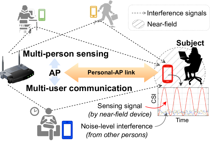
Figure 1. While each personal device uniquely identifies a person, the sensing signal (upon the person) offered by the identifying device within near-field overwhelms the interference from other persons.

In reality (as in Figure 1), each person often has its own wearable Wi-Fi devices, typically a smartphone or even a smartwatch. Although the communication link between such a personal device and the nearby Wi-Fi access point (AP) is deemed as the basic sensing media by earlier proposals on Wi-Fi human sensing, those proposals aim to leverage either a single link to perform sensing (Wang2022Placement; VitalSign-MobiHoc15; Widar2-MobiSys18; MultiSense-UbiComp20) or multiple links to offer a slightly improved spatial resolution (LiFS-MobiCom16; Widar-MobiHoc17; Widar3-MobiSys19; WiPose-MobiCom20). They all neglect two fundamental factors in such a realistic multi-user communication setting shown in Figure 1: i) each personal-AP link uniquely identifies the human subject to be sensed, and ii) since the subject is within the near-field (less than 0.2 ​m in range) of its own Wi-Fi device, the channel variation caused by its motions to its personal-AP link could be so strong as to push the interference from other subjects down to the noise floor. In other words, the default multi-user communication setting of Wi-Fi does offer the potential to be naturally extended to multi-person sensing, if one can properly integrate sensing into communication.

From application perspective, such near-field multi-person sensing naturally supports various functions under the pervasive deployment of Wi-Fi infrastructure. As these functions include sensing vital signals, gestures, activities, and locations, they are especially applicable to eXtended Reality (XR). In particular, integrating gestures and activities recognition into Wi-Fi communication reduces the peripheral sensors, leading to lighter and less power-consuming virtual reality (VR) and merged reality (MR) headsets, making them more desirable for long-time wearing (Akyildiz2022Wireless; Tan2022Commodity). Furthermore, the environmental and human sensing results indicate key contextual and localization information of nearby human and object motions; overlaying such information on the top of real-world visions facilitates augmented reality (AR) and MR applications in intrusion detection, patient monitoring, and machine status assessing (Carmigniani2011Augmented; Li2020Wireless).

Nonetheless, integrating multi-person sensing with multi-user communication is highly non-trivial, as existing practices, exploiting only artificial Wi-Fi traffic for the sensing purpose, barely offer any experience. In practice, multi-user scenarios typically cause a much lower and very irregular frame arrival rate per link, thanks to the contention-based multi-access nature of Wi-Fi. Since the CSI carried by each frame is a critical channel state sample for Wi-Fi sensing, a lower and irregular frame rate indicates a lower and irregular sampling rate, which may significantly confine the usability of Wi-Fi sensing. As most Wi-Fi sensing applications have been developed upon a high and regular frame rate (up to 1000 ​ frame/s (MultiSense-UbiComp20; Widar2-MobiSys18; WiPose-MobiCom20)), this challenge, crucial to seamless integration of multi-person sensing with multi-user communication for Wi-Fi, has never been seriously tackled.

To address these challenges, we propose MUSE-Fi as a novel MUlti-person SEnsing system leveraging Wi-Fi. To motivate MUSE-Fi, we first theoretically characterize and experimentally verify the dominating effect in near-field Wi-Fi sensing, upon which we develop criteria on the physical separability of multiple subjects. Based on the theoretical characterizations, we propose three sensing strategies for MUSE-Fi to be integrated with the traffic cross each personal-AP link, namely exploiting i) uplink (to AP) CSI, ii) downlink (from AP) CSI, and iii) downlink BFI (beamforming feedback information) (bejarano2013ieee). For all strategies, we propose a sparse recovery algorithm (SRA) to mask the potential variance in frame rate; it aims to regulate the input samples so as to deliver a unified data flow to later processing pipelines for respective sensing functions. In addition, we study the sensing effectiveness of these strategies by contrasting the BFI-enabled compressive sensing with conventional CSI-based Wi-Fi sensing. Our key contributions can be summarized as follows:

• We propose MUSE-Fi as the first true multi-person Wi-Fi sensing system; it integrates multi-person sensing with multi-user communication in a seamless manner.

• We, for the first time, expose the dominating effect of near-field Wi-Fi sensing; it is exploited by MUSE-Fi to achieve physical separation of multiple subjects.

• We design three sensing strategies for MUSE-Fi and equip them with an SRA to mask the variance in frame rate.

• We reveal the pros and cons of BFI-enabled Wi-Fi sensing against the conventional CSI-enabled one.

• We implement MUSE-Fi prototype and evaluate it with extensive experiments. The promising results confirm that MUSE-Fi indeed supports multi-person Wi-Fi sensing under realistic scenarios.

The rest of the paper is organized as follows. Section 2 discusses the dominating effect of near-field sensing both theoretically and experimentally. Section LABEL:sec:design presents the sensing strategies for MUSE-Fi, along with the crucial SRA to regulate the frame rate. Section LABEL:sec:implementation specifies how the MUSE-Fi prototype is implemented and how the application scenarios for case studies are set up. Section LABEL:sec:evaluation reports the evaluation results of three case studies. Related works are briefly discussed in Section LABEL:sec:related_work. Finally, Section LABEL:sec:conclusion concludes our paper.

2. Sensing by Near-field Domination

In this section, we introduce the Wi-Fi human sensing basics, and systematically study and validate the dominating signal variations in near-field sensing. Compared with conventional antenna near-field and capacitive coupling (Balanis2016Antenna; Grosse2014Capacitive) not developed for practical multi-person sensing, our theoretical analyses allow for characterizing the feasible region of near-field sensing and shedding insights on the upper/lower bounds of subject number and spacing.

2.1. Wi-Fi Human Sensing Basics

We start by introducing a Wi-Fi sensing system with an AP and user equipment (UE) pair aiming to sense the physical motion of a human subject denoted by $\mathcal{S}$. At time $t$, denote the distance between the AP and S by $d_{A,\lx@glossaries@gls@link{main}{tar}{\leavevmode\mathcal{S}}}(t)$ and the distance between S and the UE by $d_{\lx@glossaries@gls@link{main}{tar}{\leavevmode\mathcal{S}},E}(t)$. Further focusing on the influence of $\mathcal{S}$, we model the wireless channel gain between the AP and the UE as:

(1) $$h_{A,E}(t)=h_{A,\lx@glossaries@gls@link{main}{tar}{\leavevmode\mathcal{S}},E}(t)+h_{A,E}^{S}+h_{A,E}^{D}(t),$$

where $h_{A,E}^{S}$ and $h_{A,E}^{D}(t)$ represent the static and dynamic channel gains between the AP and UE due to, respectively, the direct communication path and interfering motions along it, and $h_{A,\lx@glossaries@gls@link{main}{tar}{\leavevmode\mathcal{S}},E}(t)$ indicates the channel gain from the AP to UE via the reflection of S, which can be expressed as:

(2) $$\!\!\!h_{A,\lx@glossaries@gls@link{main}{tar}{\leavevmode\mathcal{S}},E}(t)=\frac{\lambda^{2}\sqrt{G_{A,\lx@glossaries@gls@link{main}{tar}{\leavevmode\mathcal{S}},E}}\exp(-\mathrm{i}{2\pi}(d_{A,\lx@glossaries@gls@link{main}{tar}{\leavevmode\mathcal{S}}}(t)+d_{\lx@glossaries@gls@link{main}{tar}{\leavevmode\mathcal{S}},E}(t))/{\lambda})}{(4\pi)^{2}(d_{A,\lx@glossaries@gls@link{main}{tar}{\leavevmode\mathcal{S}}}(t)d_{\lx@glossaries@gls@link{main}{tar}{\leavevmode\mathcal{S}},E}(t))^{\alpha/2}},$$

where $\lambda$ is the carrier wavelength, $G_{A,\lx@glossaries@gls@link{main}{tar}{\leavevmode\mathcal{S}},E}$ represents the product of Tx and Rx antenna gains and the reflection coefficient of $\mathcal{S}$, and $\alpha$ is the path loss exponent (goldsmith2005wireless). Typically, $\alpha\in[2,4]$ with $\alpha\approx 4$ for indoor environments (rappaport2010wireless). Therefore, Wi-Fi human sensing can be described as follows: the physical motion of a human subject results in changes of $d_{A,\lx@glossaries@gls@link{main}{tar}{\leavevmode\mathcal{S}}}(t)$ and $d_{\lx@glossaries@gls@link{main}{tar}{\leavevmode\mathcal{S}},E}(t)$, which in turn lead to the changes of channel gain $h_{A,\lx@glossaries@gls@link{main}{tar}{\leavevmode\mathcal{S}},E}(t)$ over time. Therefore, by analyzing the time series of $h_{A,\lx@glossaries@gls@link{main}{tar}{\leavevmode\mathcal{S}},E}(t)$ obtained from the CSI of the Wi-Fi frames, both AP and UE are able to sense the motion of $\mathcal{S}$.

2.2. Feasible Region for Near-field Sensing

Consider a more general scenario where two persons exist in the Wi-Fi sensing system. Without loss of generality, we let one of them be the subject $\mathcal{S}$, and refer to the other as the interferer denoted by $\mathcal{I}$. Consequently, the channel gain between the AP and UE in Eqn. (1) becomes:

(3) $$\tilde{h}_{A,E}(t)=h_{A,\lx@glossaries@gls@link{main}{tar}{\leavevmode\mathcal{S}},E}(t)+h_{A,\lx@glossaries@gls@link{main}{int}{\leavevmode\mathcal{I}},E}(t)+h_{A,E}^{S}+h_{A,E}^{D}(t),$$

where $h_{A,\lx@glossaries@gls@link{main}{int}{\leavevmode\mathcal{I}},E}(t)$ is the channel gain from the AP to UE via the reflection of I; it can be modeled in a similar manner as Eqn. (2). Eqn. (3) seems to suggest that it is hard to separate the channel influences imposed by $\mathcal{S}$ and $\mathcal{I}$ since their channel gains get mixed up. Nevertheless, we point out that, in the Wi-Fi sensing scenarios where $\mathcal{S}$ is close to or in the near-field of UE (i.e., distance below 0.2 ​m, empirically), the variation of the channel gain is dominated by the $\mathcal{S}$’s physical motion; in other words, $\partial|h_{A,\lx@glossaries@gls@link{main}{tar}{\leavevmode\mathcal{S}},E}(t)|/\partial t\gg\partial|h_{A,\lx@glossaries@gls@link{main}{int}{\leavevmode\mathcal{I}},E}(t)|/\partial t$. We term this phenomenon near-field domination effect, and we provide its theoretical analysis as follows.

Firstly, to quantify the variation of $h_{A,\lx@glossaries@gls@link{main}{tar}{\leavevmode\mathcal{S}},E}(t)$, we evaluate it by the squared amplitude of the partial derivative of $h_{A,\lx@glossaries@gls@link{main}{tar}{\leavevmode\mathcal{S}},E}(t)$ w.r.t. $t$, which is referred to as the power of channel variation. To simplify the analysis, we assume $\partial d_{A,\lx@glossaries@gls@link{main}{tar}{\leavevmode\mathcal{S}}}(t)/\partial t=\partial d_{\lx@glossaries@gls@link{main}{tar}{\leavevmode\mathcal{S}},E}(t)/\partial t=v_{\lx@glossaries@gls@link{main}{tar}{\leavevmode\mathcal{S}}}$. The value of $v_{\lx@glossaries@gls@link{main}{tar}{\leavevmode\mathcal{S}}}$ can be interpreted as the intensity of $\mathcal{S}$’s motion in terms of speed. The power of channel variation of $\mathcal{S}$ can then be calculated as:

$$P_{\lx@glossaries@gls@link{main}{tar}{\leavevmode\mathcal{S}}} =\left|\frac{\partial h_{A,\lx@glossaries@gls@link{main}{tar}{\leavevmode\mathcal{S}},E}(t)}{\partial t}\right|^{2}$$

$$\approx\frac{{G_{A,\lx@glossaries@gls@link{main}{tar}{\leavevmode\mathcal{S}},E}}\lambda^{4}v_{\lx@glossaries@gls@link{main}{tar}{\leavevmode\mathcal{S}}}^{2}}{(4\pi)^{4}(d_{A,\lx@glossaries@gls@link{main}{tar}{\leavevmode\mathcal{S}}}d_{\lx@glossaries@gls@link{main}{tar}{\leavevmode\mathcal{S}},E})^{\alpha}}\left[\frac{\alpha^{2}}{4}\Big{(}\frac{d_{A,\lx@glossaries@gls@link{main}{tar}{\leavevmode\mathcal{S}}}+d_{\lx@glossaries@gls@link{main}{tar}{\leavevmode\mathcal{S}},E}}{d_{A,\lx@glossaries@gls@link{main}{tar}{\leavevmode\mathcal{S}}}d_{\lx@glossaries@gls@link{main}{tar}{\leavevmode\mathcal{S}},E}}\Big{)}^{2}+\frac{16\pi^{2}}{\lambda^{2}}\right]$$

(4) $$\stackrel{{\scriptstyle(\star)}}{{\approx}}{\tilde{G}_{A,\lx@glossaries@gls@link{main}{tar}{\leavevmode\mathcal{S}},E}}\cdot v_{\lx@glossaries@gls@link{main}{tar}{\leavevmode\mathcal{S}}}^{2}\cdot{(d_{A,\lx@glossaries@gls@link{main}{tar}{\leavevmode\mathcal{S}}}d_{\lx@glossaries@gls@link{main}{tar}{\leavevmode\mathcal{S}},E})^{-\alpha}},$$

where we omit symbol $t$ in the distance notations and let $\tilde{G}_{A,\lx@glossaries@gls@link{main}{tar}{\leavevmode\mathcal{S}},E}=(\lambda/4\pi)^{2}G_{A,\lx@glossaries@gls@link{main}{tar}{\leavevmode\mathcal{S}},E}$ for the sake of brevity. In the second row of Eqn. (2.2), the first term inside the bracket is caused by the amplitude variation of the channel gain and the second term results from the phase variation of the channel gain. $(\star)$ holds because, in typical 5 ​GHz Wi-Fi sensing systems with $\mathcal{S}$ in the near-field of UE (e.g., $d_{A,\lx@glossaries@gls@link{main}{tar}{\leavevmode\mathcal{S}}}\!\sim\!3$ ​m, $d_{\lx@glossaries@gls@link{main}{tar}{\leavevmode\mathcal{S}},E}\!\sim\!0.1$ ​m, and $\lambda\!\sim\!0.06$ ​m), the first term in the bracket is much smaller than the second term and thus can be omitted, implying that the channel variation is mainly due to that $\mathcal{S}$’s motion changes the phase of the channel.

The power of variation of $h_{A,\lx@glossaries@gls@link{main}{int}{\leavevmode\mathcal{I}},E}(t)$ can be similarly derived for $\mathcal{I}$ as $P_{\lx@glossaries@gls@link{main}{int}{\leavevmode\mathcal{I}}}=\tilde{G}_{A,\lx@glossaries@gls@link{main}{int}{\leavevmode\mathcal{I}},E}v_{\lx@glossaries@gls@link{main}{int}{\leavevmode\mathcal{I}}}^{2}(d_{A,\lx@glossaries@gls@link{main}{int}{\leavevmode\mathcal{I}}}d_{\lx@glossaries@gls@link{main}{int}{\leavevmode\mathcal{I}},E})^{-\alpha}$, with $d_{A,\lx@glossaries@gls@link{main}{int}{\leavevmode\mathcal{I}}}$ and $d_{\lx@glossaries@gls@link{main}{int}{\leavevmode\mathcal{I}},E}$ being the distance between the AP and $\mathcal{I}$ and between $\mathcal{I}$ and the UE, respectively, and $v_{\lx@glossaries@gls@link{main}{int}{\leavevmode\mathcal{I}}}$ being the intensity. Consequently, the near field domination effect can be interpreted as $P_{\lx@glossaries@gls@link{main}{tar}{\leavevmode\mathcal{S}}}$ being significantly larger than $P_{\lx@glossaries@gls@link{main}{int}{\leavevmode\mathcal{I}}}$, thanks to $d_{\lx@glossaries@gls@link{main}{tar}{\leavevmode\mathcal{S}},E}$ being much smaller than $d_{\lx@glossaries@gls@link{main}{int}{\leavevmode\mathcal{I}},E}$, given $d_{A,\lx@glossaries@gls@link{main}{tar}{\leavevmode\mathcal{S}}}\approx d_{A,\lx@glossaries@gls@link{main}{int}{\leavevmode\mathcal{I}}}$ and $v_{\lx@glossaries@gls@link{main}{tar}{\leavevmode\mathcal{S}}}\approx v_{\lx@glossaries@gls@link{main}{int}{\leavevmode\mathcal{I}}}$. It is worth noting that assuming $v_{\lx@glossaries@gls@link{main}{tar}{\leavevmode\mathcal{S}}}\approx v_{\lx@glossaries@gls@link{main}{int}{\leavevmode\mathcal{I}}}$ may not be practical, because human sensing to different targets may have distinct meaning (e.g., respiration monitoring against gesture detection). Though our following derivation shall stick to this symmetric assumption for the ease of exposition, we will experimentally validate that the near-field domination still holds even with asymmetric intensities, as far as there is a sufficient discrepancy between $d_{\lx@glossaries@gls@link{main}{tar}{\leavevmode\mathcal{S}},E}$ and $d_{\lx@glossaries@gls@link{main}{int}{\leavevmode\mathcal{I}},E}$.

In order to concretely characterize the interferer’s feasible region that maintains the domination of $P_{\lx@glossaries@gls@link{main}{tar}{\leavevmode\mathcal{S}}}$ at the UE, we propose an novel metric variation to interference ratio (VIR); it evaluates the variation power ratio between $h_{A,\lx@glossaries@gls@link{main}{tar}{\leavevmode\mathcal{S}},E}(t)$ and the sum of $h_{A,\lx@glossaries@gls@link{main}{int}{\leavevmode\mathcal{I}},E}(t)$ and dynamic channel $h_{A,E}^{D}(t)$. Based on (Wang2022Placement), $h_{A,E}^{D}(t)$ can be also treated as an interference, whose power $P_{d}$ is in linear proportion to that of the static channel gain. Therefore, assuming a LoS path between the AP and UE, we have $P_{d}=\eta{\lambda}^{2}{d_{A,E}}^{-\alpha}+b$, where $\eta$ and $b$ are fixed for a given pair of AP and UE. Then, we have:

(5)