Static and Dynamic BART for Rank-Order Data

Abstract

Ranking lists are often provided at regular time intervals by one or multiple rankers in a range of applications, including sports, marketing, and politics. Most popular methods for rank-order data postulate a linear specification for the latent scores, which determine the observed ranks, and ignore the temporal dependence of the ranking lists. To address these issues, novel nonparametric static (ROBART) and autoregressive (ARROBART) models are introduced, with latent scores defined as nonlinear Bayesian additive regression tree functions of covariates.

To make inferences in the dynamic ARROBART model, closed-form filtering, predictive, and smoothing distributions for the latent time-varying scores are derived. These results are applied in a Gibbs sampler with data augmentation for posterior inference.

The proposed methods are shown to outperform existing competitors in simulation studies, and the advantages of the dynamic model are demonstrated by forecasts of weekly pollster rankings of NCAA football teams.

Keywords: Autoregressive Process; BART; Filtering and Smoothing; Rank-Order Data; Thurstone model

1 Introduction

Rank-order data emerge when an expert is asked to rank a finite set of $N$ alternatives, or items, according to a certain criterion, such as personal preference or a predetermined statistic. The study of rank-order data is becoming popular in several fields, including political science (Gormley and Murphy, 2008), music preferences (Bradlow and Fader, 2001), economics (Fok et al., 2012), and sports analytics (Graves et al., 2003). In practice, the rankers are likely heterogeneous in their qualities or opinions, and it is often of interest to investigate how the rankings may be dependent on covariates of the ranked items (e.g., summary statistics). For example, for sports leagues such as the NCAA, NFL, or NBA, many experts provide ranking lists of teams by relying on their experiences and team-specific statistics, like the win percentage and the margin of victory. Moreover, reflecting the inherently dynamic nature of competitors’ abilities and human preferences, the experts’ rankings may change over time (e.g., Graves et al., 2003). Analogous considerations hold for rank-order data from other fields, such as marketing, politics, and health economics.

In this article, we focus on models for rank-order data, also called order-statistics models (Alvo and Philip, 2014; Liu et al., 2019). Specifically, we consider the family of Thurstone models, which assumes the existence of an unobserved evaluation score for each of the $N$ items whose noisy versions determine the rankings provided by the $M$ experts. However, most of the existing models in this class are designed to study cross-sectional data and are inherently static, thus ignoring any temporal dependence.

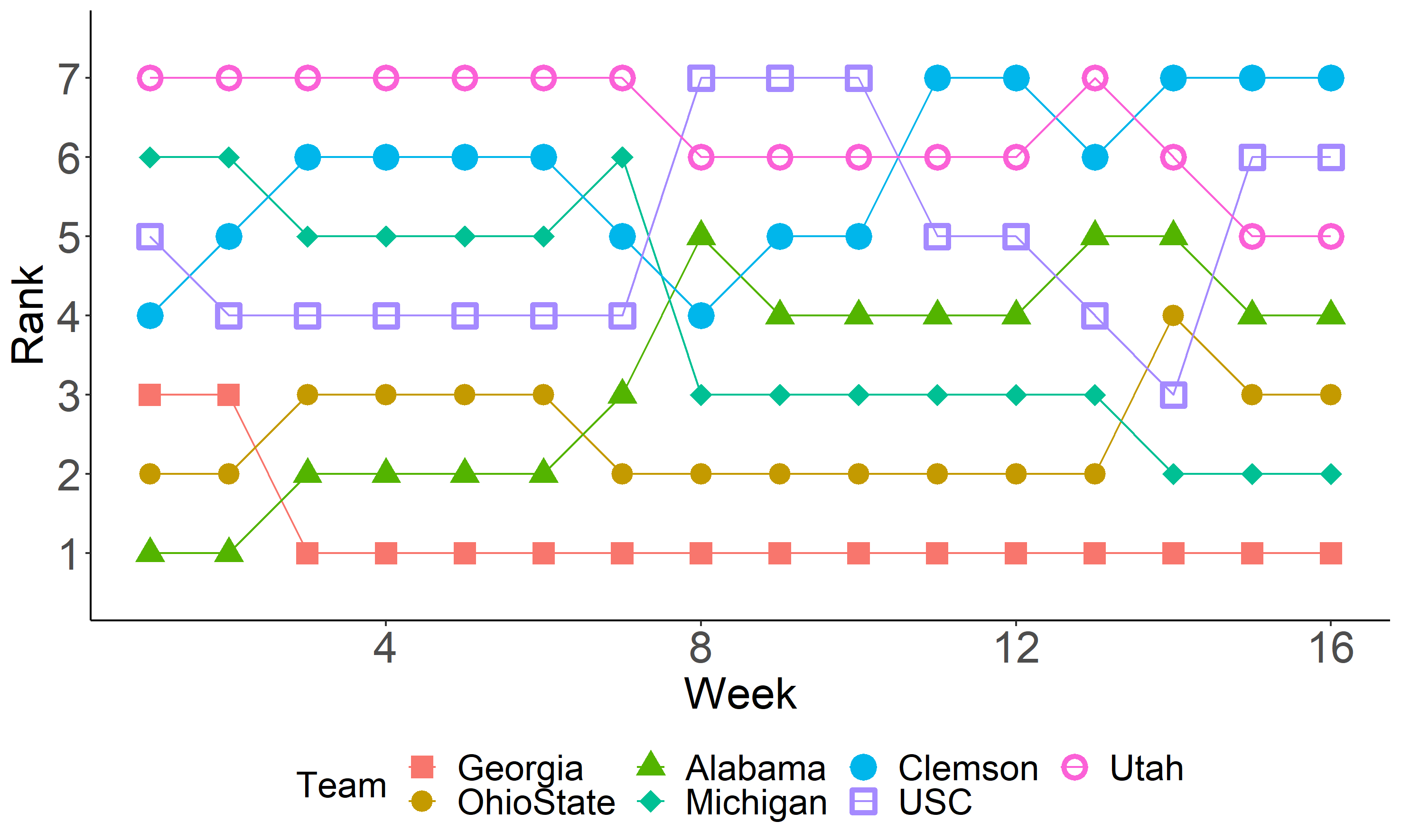
Figure 1: AP Pollster Brian Howell: Observed relative ranks for $N=7$ teams of the 2022 NCAA Division I Football season.

Figure 1 shows the time-varying ranking list of a single pollster from the 2022 NCAA Division I Football season, which will be investigated in Section 5. First, all teams are ranked each week, where the temporal evolution is highlighted by the colored lines. Second, the overall ranking list seems persistent over time. Third, the shifts in the ranking are heterogeneous in magnitude, as both large and small changes are observed. Overall, this suggests that a team’s ranking is rather stable within the season, with small changes driven by the slow evolution of teams’ abilities and sporadic large breaks often due to sudden events, such as players’ injuries and coach replacements. Similar features are found in other rank-order data, such as political voting or customer preferences.

The main challenge in investigating and forecasting this class of data is the constraint among the items in a ranking list (or time series of them), which prevents the use of equation-by-equation modeling and calls for specific statistical tools. However, the existing rank-order models fall short of the flexibility necessary (i) to address the highly nonlinear relationship between the item’s features and observed rankings and (ii) to forecast time series characterized by possibly large changes.

This article contributes to the literature on rank-order models by proposing two new methods for addressing these issues. Specifically, we leverage the Bayesian additive regression trees (BART, see Chipman et al., 2010) framework to define a flexible nonparametric static model for rank-order data, named rank-order Bayesian additive regression trees (ROBART). Then, we extend this framework to a dynamic model called autoregressive rank-order Bayesian additive regression trees (ARROBART), which accounts for the persistence in time series of rank-order data (e.g., see Fig. 1).

The most widely used families of models for rank data are the Thurstone (Thurstone, 1927) and Plackett-Luce (Luce, 1959; Plackett, 1975), which differ in the distribution of the noise in the random utility representations (normal and Gumbel, respectively) and in the ordering interpretation (joint or sequential). Relying on normal regression models makes the Thurstone family easier to interpret and extend in several directions. However, the estimation of these models is generally difficult, especially for large numbers of ranked items, due to the high-dimensional integral form of the likelihood function. Within the Thurstone family, the Bayesian approach coupled with data augmentation methods provides an advantageous computational alternative that also allows for the introduction of covariates (Yu, 2000). Johnson et al. (2002) developed a hierarchical Bayesian Thurstone model for rank-order data from known groups of evaluators, whereas Li et al. (2022) propose a Thurstone model with ranker-specific error variances and a Dirichlet process mixture prior for ranker-specific effects of covariates. Recently, Gu and Yu (2023) introduce a Bayesian spatial autoregressive model to learn ranking data in social networks and to account for social dependencies among individuals. We contribute to this literature by proposing two new Thurstone models, a static and a dynamic one, where a Bayesian nonparametric approach is used to capture the possibly nonlinear impact of covariates.

The study of time series of rankings is less developed but has attracted increasing attention in recent years. Most existing dynamic ranking models are generalizations of the Plackett-Luce model (Bradlow and Fader, 2001; Grewal et al., 2008; Glickman and Hennessy, 2015; Henderson and Kirrane, 2018), whereas this article provides a dynamic extension to the Thurstone family. Specifically, we propose a novel time-varying nonparametric approach that considers an autoregressive process for the latent scores and uses a specification based on regression trees to flexibly model the impact of the lagged response and the external covariates. Its linear counterpart is also introduced as a benchmark.

The possibility of having large deviations as well as small changes in the time series of ranking lists, as shown in Fig. 1, calls for the use of flexible tools to model the dynamics of the latent teams’ scores. To address these issues, we introduce for the first time the BART specification in order-statistics models to design static and dynamic nonparametric frameworks for rank-order data. Bayesian additive regression trees provide a powerful approach for fitting and forecasting regression models while avoiding parametric assumptions; see Hill et al. (2020) for an overview of the most popular extensions. Despite its advantages, BART has rarely been used in time series or state space models. Recent advances include Bayesian additive vector autoregressive trees for multiple time series (Huber and Rossini, 2022), and an extension to a mixed-frequency context for nowcasting in the presence of extreme observations (Huber et al., 2023) .

Our contribution to this literature concerns the derivation of new closed-form filtering, predictive, and smoothing distributions for the latent time-varying scores in the ARROBART model. Furthermore, we show the proportionality of these distributions to finite mixtures. These results, coupled with a data augmentation approach, are crucial to designing a Gibbs sampler for posterior inference.

The proposed ROBART and ARROBART models are tested on static and dynamic synthetic datasets, respectively, highlighting the superior performance against their linear counterparts as well as other existing methods. The proposed models are then used to forecast NCAA Division I football poll data, of which Fig. 1 shows the time series provided by a single pollster. We find strong evidence supporting the dynamic nonlinear ARROBART model against the dynamic linear and static counterparts, thus suggesting the importance of accounting for temporal persistence and nonlinearities.

The remainder of the article is organized as follows: Section 2 provides an overview of the Thurstone model and illustrates the ROBART and the ARROBART models. It also provides a theorem describing the filtering and smoothing distributions for ARROBART. Section 3 presents a Bayesian approach to inference. Section 4 investigates the performance of our methods on simulated data, then Section 5 shows the results of an application to real data on NCAA College Football team rankings. Section 6 concludes the article.

2 Nonparametric Thurstone Models for Rank-Order Data

This section introduces the notation on ranking lists, then it presents a new class of nonparametric models for rank-order data that extends the Thurstone model (Thurstone, 1927) by allowing for flexible, possibly nonlinear functions of the covariates. Then, we extend the framework to account for temporal dependence and persistence for investigating and forecasting time series data.

A full ranking of $N$ items is a mapping $\tau:\mathds{A}\to\mathcal{P}_{N}$ from a finite, ordered set of alternatives/items, $\mathds{A}=\{a_{1},\ldots,a_{N}\}$ to the space of $N$-dimensional permutations, $\mathcal{P}_{N}$. Let $\#$ denote the cardinality of a set. With a slight abuse of notation, we denote a full ranking of $N$ items by the vector $\tau=(\tau_{1},\ldots,\tau_{N})^{\prime}\in\mathcal{P}_{N}$, where $\tau_{i}=\tau(i)$ is the rank of item $a_{i}\in\mathds{A}$, for $i=1,\ldots,N$, and $\tau_{i}<\tau_{j}$ means that alternative $a_{i}$ is preferred to $a_{j}$, written $a_{i}\succ a_{j}$ since it is assigned a lower rank. Rankings and pairwise comparisons are related, as, given a full ranking $\tau$, it holds $[a_{i}\succ a_{j}]\iff\tau_{i}<\tau_{j}$ for each $i,j\in\{1,\ldots,N\}$. Therefore, a full ranking $\tau$ is an ordered $N$-tuple representing a set of non-contradictory pairwise relationships in $\mathds{A}$, and as such, it encodes an ordered preference for all the items in $\mathds{A}$.

In this article, we consider a setting where $N$ items are ordered by $M$ rankers. For each item $i=1,\ldots,N$ and ranker $j=1,\ldots,M$, the $K_{x}$-dimensional vector of covariates is denoted by $\mathbf{X}_{ij}\in\mathds{R}^{K_{x}}$. In the dynamic case, this setup is replicated for each of the $T$ time periods. Finally, for any vector $\mathbf{z}=(z_{1},\ldots,z_{N})^{\prime}\in\mathds{R}^{N}$, we use $\operatorname{rank}(\mathbf{z})=[a_{i_{1}}\succ\ldots\succ a_{i_{N}}]$ to denote the full ranking of $z_{i}$’s in decreasing order of preference, that is, $z_{i_{1}}<\ldots<z_{i_{N}}$.

2.1 Overview of Bayesian Additive Regression Trees

A Bayesian additive regression tree (BART) specification for a function $f:\mathds{R}^{K_{x}}\to\mathds{R}$ is a hierarchical prior that approximates $f$ by means of a sum of regression trees. Let us denote by $\mathcal{T}$ a binary tree consisting of a set of interior node decision rules and a set of terminal nodes (or leaves), and let $\bm{\mu}=\{\mu_{1},\ldots,\mu_{b}\}$ be a set of parameter values associated with each of the $b$ terminal nodes of $\mathcal{T}$. A regression tree takes covariate values as input and produces a fitted outcome value given by the parameter associated with a terminal node of the tree. This outcome is obtained by dividing the domain of the covariate $\mathbf{x}_{i}=(x_{i1},\ldots,x_{iK_{x}})^{\prime}\in\mathds{R}^{K_{x}}$ into disjoint regions $\{B_{\ell}\}_{\ell=1}^{b}$ using a sequence of binary rules of the form $\{\mathbf{x}_{i}\in A_{h}\}$ versus $\{\mathbf{x}_{i}\notin A_{h}\}$, where $h\in\mathcal{I}$ indexes the internal nodes of the tree. Most commonly, $A_{h}$ is defined by a splitting variable $k_{h}$ and splitting point $c_{h}$, such as $A_{h}=\{\mathbf{x}_{i}:x_{ik_{h}}\leq c_{h}\}$. Then, $\mathbf{x}_{i}$ is assigned the value $\mu_{\ell}$, with $\ell\in\{1,\ldots,b\}$, associated with a single terminal node $B_{\ell}$ of $\mathcal{T}$ defined by a sequence of decision rules.

A tree $\mathcal{T}$ and a collection of leaf parameters $\bm{\mu}$ define a step function $g(\mathbf{x}_{i}|\mathcal{T},\bm{\mu})$ that assigns value $\mu_{\ell}\in\bm{\mu}$ to $\mathbf{x}_{i}$, thus resulting in:

$$g(\mathbf{x}_{i}|\mathcal{T},\bm{\mu})=\sum_{\ell=1}^{b}\mu_{\ell}\mathbb{I}(\mathbf{x}_{i}\in B_{\ell}),$$

where $\mathbb{I}(\cdot)$ is the indicator function and $\{B_{\ell}\}_{\ell=1}^{b}$ is the partition of the domain of the covariate $\mathbf{x}_{i}$ associated to the tree $\mathcal{T}$. The BART specification consists in approximating the function $f$ through a sum of $S$ trees, as follows:

$$f(\mathbf{x}_{i})\approx\sum_{s=1}^{S}g_{s}(\mathbf{x}_{i}|\mathcal{T}_{s},\bm{\mu}_{s})=\sum_{s=1}^{S}\sum_{\ell=1}^{b_{s}}\mu_{\ell,s}\mathbb{I}(\mathbf{x}_{i}\in B_{\ell,s}),$$ (1)

where $g_{s}$ is a tree function that assigns $\mu_{\ell,s}\in\bm{\mu}_{s}$ to $\mathbf{x}_{i}$ for each binary regression tree $\mathcal{T}_{s}$.

2.2 Static Model: Rank-Order BART

The Thurstone model can be described as a random utility model (e.g., see Walker and Ben-Akiva, 2002), where the full ranking $\tau$ is driven by a latent score, $\mathbf{z}$, such that for any two items $i_{1},i_{2}$, it holds $z_{i_{1}}<z_{i_{2}}$ if and only if $i_{1}\succ i_{2}$. The latent vector $\mathbf{z}$ is assumed to follow a multivariate normal distribution with mean $\bm{\gamma}=(\gamma_{1},\ldots,\gamma_{N})^{\prime}$ representing the score of each item:

$$\begin{split}\tau&=\operatorname{rank}(\mathbf{z}),\qquad z_{i}=\gamma_{i}+\varepsilon_{i},\qquad\varepsilon_{i}\sim\mathcal{N}(0,\sigma_{\varepsilon}^{2}).\end{split}$$ (2)

The model in Eq. (2) poses an identification problem since the observations only provide information about the ordering of the elements in $\mathbf{z}$, which implies that the parameters $(\bm{\gamma},\sigma_{\varepsilon}^{2})$ are not separately identifiable from the likelihood. Therefore, to ensure the identification of the parameters, we fix $\sigma_{\varepsilon}^{2}=1$.

Consider a framework where no temporal observations are available or the time dependence is irrelevant to the analysis. Moreover, we assume each individual in a collection of $M$ professionals or rankers provides a ranking list of the same set of $N$ items, as is common in many real-world situations such as sports analytics and customer reviews. To investigate data without temporal dependence, we define a new static model that extends the Thurston approach in Eq. (2) by including the BART specification from Eq. (1) for the conditional mean of the latent scores. Specifically, we generalise Eq. (2) by assuming ranker-specific scores, $\mathbf{z}_{j}$. To account for external information that might affect the rankers’ decision process, we can include item- and ranker-specific covariates, $\mathbf{x}_{i}^{a}\in\mathds{R}^{K_{a}}$ and $\mathbf{x}_{j}^{r}\in\mathds{R}^{K_{r}}$, as well as covariates specific to both alternatives and rankers, $\mathbf{w}_{ij}\in\mathds{R}^{K_{w}}$. Then, for each pair $(i,j)$, we replace the intercept $\gamma_{ij}$ with an unknown function of the covariates, $f$. Moreover, to cope with potential deviations from linearity and to allow for wide changes in the dynamics of the rankers’ score, we adopt a nonparametric approach based on a BART specification for the latent regression function, $f$.

For each item $i=1,\ldots,N$ and ranker $j=1,\ldots,M$, let $\mathbf{\tilde{X}}_{ij}=(\mathbf{x}_{i}^{a\prime},\mathbf{x}_{j}^{r\prime},\mathbf{w}_{ij}^{\prime})^{\prime}\in\mathds{R}^{K_{x}}$ be a covariate vector. The Rank-Order BART model (ROBART) is defined as:

$$\begin{split}\tau_{j}=\operatorname{rank}(\mathbf{z}_{j}),\qquad z_{ij}&=f(\mathbf{\tilde{X}}_{ij})+\varepsilon_{ij},\qquad\varepsilon_{ij}\mathbin{\overset{iid}{\kern 0.0pt\sim}}\mathcal{N}(0,1),\\ f(\mathbf{\tilde{X}}_{ij})&=\sum_{s=1}^{S}\sum_{\ell=1}^{b_{s}}\mu_{\ell,s}\mathbb{I}(\mathbf{\tilde{X}}_{ij}\in B_{\ell,s}),\end{split}$$ (3)

where $f:\mathds{R}^{K_{x}}\to\mathds{R}$ is a regression function for which we assume a BART specification. Denoting with $\delta_{\mathbf{z}}(\tau)$ the Dirac mass at $\mathbf{z}$, $\left\lVert\cdot\right\rVert$ the $L_{2}$ norm, and $\bm{\theta}$ a vector collecting the ranker-specific parameters, one obtains the likelihood:

$$\begin{split}L(\tau_{1},\ldots,\tau_{M}|\bm{\theta})&=\prod_{j=1}^{M}\int_{\mathds{R}^{N}}(2\pi)^{-\frac{N}{2}}\exp\Bigg{(}-\frac{\big{\|}\mathbf{z}_{j}-f(\mathbf{\tilde{X}}_{ij})\big{\|}^{2}}{2}\Bigg{)}\delta_{\operatorname{rank}(\mathbf{z}_{j})}(\tau_{j})\>\mathrm{d}\mathbf{z}_{j}.\end{split}$$ (4)

2.3 Dynamic Model: AutoRegressive Rank-Order BART

In many real-world cases, multiple professionals continuously evaluate the alternatives and provide their ranking lists periodically over time. The latent scores that a ranker assigns to each item, which ultimately determine the professional’s ranking lists observed by the researcher, evolve over time to reflect the change in the information set and in the features of the alternatives. Nonetheless, most of the existing models for rank-order data disregard the temporal dimension of the data, thus missing information on the serial correlation in the rankers’ latent scores and observed ranks. We aim to address this issue by proposing a modification of the Thurstone model that accounts for the temporal persistence of the ranking lists as implied by an evolution of the underlying rankers’ scores.

Suppose that each ranker provides a ranking of alternatives at each time $t=1,\ldots,T$, and let $\tau_{j,t}$ denote the observed ranking list of ranker $j$ in period $t$. Moreover, let $\mathbf{z}_{j,t}=(z_{1j,t},\ldots,z_{Nj,t})^{\prime}$, where $z_{ij,t}$ denotes the unobserved ranker $j$’s score for alternative $i$, such that $z_{i_{1}j,t}>z_{i_{2}j,t}$ if and only if $i_{1}\prec i_{2}$ for ranker $j$ at time $t$. In this setting, each latent score $z_{ij,t}$ can be modeled as an unknown function $f$ of its first lag and the external covariates. This is done by considering the covariate vector $\mathbf{X}_{ij,t}=(z_{ij,t-1},\mathbf{x}_{i,t}^{a\prime},\mathbf{x}_{j,t}^{r\prime},\mathbf{w}_{ij,t}^{\prime})^{\prime}\in\mathds{R}^{K_{x}}$, where $\mathbf{x}_{i,t}^{a}$, $\mathbf{x}_{j,t}^{r}$, and $\mathbf{w}_{ij,t}$ are the item-, ranker-, and item/ranker-specific variables.

Therefore, in the presence of time series rank-order data where temporal persistence is a relevant feature, we extend the ROBART model in Eq. (3) to a dynamic framework by defining an AutoRegressive Rank-Order BART model with exogenous covariates (ARROBARTX) as follows:

$$\begin{split}\tau_{j,t}=\operatorname{rank}(\mathbf{z}_{j,t}),\qquad z_{ij,t}&=f(\mathbf{X}_{ij,t})+\varepsilon_{ij,t},\qquad\varepsilon_{ij,t}\mathbin{\overset{iid}{\kern 0.0pt\sim}}\mathcal{N}(0,1),\\ f(\mathbf{X}_{ij,t})&=\sum_{s=1}^{S}\sum_{\ell=1}^{b_{s}}\mu_{\ell,s}\mathbb{I}(\mathbf{X}_{ij,t}\in B_{\ell,s}),\end{split}$$ (5)

where the regression function $f$ is approximated by a BART specification. A special case of the ARROBARTX in Eq. (5) is an AutoRegressive Rank-Order BART model without covariates (ARROBART) and with one lag, which is obtained by assuming $\mathbf{X}_{ij,t}=\mathbf{z}_{j,t-1}$. The ARROBART model can be interpreted as a hidden Markov model (HMM, see Cappé et al., 2005) with measurement and transition density given by, respectively:

$$\tau_{j,t}|\mathbf{z}_{j,t} \sim\delta_{\operatorname{rank}(\mathbf{z}_{j,t})}(\tau_{j,t}),$$

$$\mathbf{z}_{j,t}|\mathbf{z}_{j,t-1} \sim\mathcal{N}_{N}(\mathbf{z}_{j,t}|f(\mathbf{z}_{j,t-1}),I_{N}),$$

where $f$ is approximated by a BART and $I_{N}$ denotes the $N$-dimensional identity matrix. Let $\bm{\tau}=\{\tau_{j,t}:j\in\{1,\dots,M\},t\in\{1,\dots,T\}\}$ denote the collection of all the observations and $\bm{\theta}$ be the collection of all parameters. The ARROBART likelihood function is:

$$L(\bm{\tau}|\bm{\theta})=\prod_{j=1}^{M}\underbrace{\int_{\mathds{R}^{N}}\dots\int_{\mathds{R}^{N}}}_{\text{T+1 integrals}}\left(\prod_{t=1}^{T}p(\tau_{j,t}|\mathbf{z}_{j,t})p(\mathbf{z}_{j,t}|\mathbf{z}_{j,t-1},\bm{\theta})\right)p(\mathbf{z}_{j,0}|\bm{\theta})\>\mathrm{d}\mathbf{z}_{j,0}\dots\mathrm{d}\mathbf{z}_{j,T},$$ (6)

where $\mathbf{z}_{j,0}$ is the initial value of the latent vector. As the ARROBART model postulates independence across rankers $j$, hereafter, without loss of generality, we focus on the case $M=1$ and drop the corresponding index.

The temporal dependence among the latent variables introduces a filtering problem in the estimation of the ARROBART model, as making inferences on the latent vector $\mathbf{z}_{t}$ requires the derivation of appropriate filtering and smoothing distributions.

Let us first introduce some additional notation. For a variable $x\in\mathcal{D}\subseteq\mathds{R}$, the BART specification induces a partition $\{C_{k}\}_{k=1}^{K}$ of the domain $\mathcal{D}$ (see the Supplement for a proof). Notice that $\{B_{\ell,s}\}_{\ell=1}^{b_{s}}$ is a partition of $\mathcal{D}$ for each tree $s\in\{1,\ldots,S\}$, where the $\ell$th leaf of the $s$th tree is associated to a scalar coefficient $\mu_{\ell,s}\in\mathds{R}$. Let us define a one-to-one map that associates each tuple $(j_{1},\ldots,j_{S})\in\mathop{\mathchoice{\vbox{\hbox to10.03749pt{\vrule height=15.05624pt,width=0.0pt\hss}}}{\vbox{\hbox to10.03749pt{\kern 1.00374pt\vrule height=10.03749pt,width=0.0pt\hss}}}{\times}{\times}}_{s=1}^{S}\{1,\ldots,b_{s}\}$ to an index $k\in\{1,\ldots,K\}$, where $K=\sum_{s=1}^{S}b_{s}$ is the total number of the tuples. Then, for each tuple $(j_{1},\ldots,j_{S})$ and associated $k$ index, define $C_{k}=B_{j_{1},1}\cap\ldots\cap B_{j_{S},S}$ and let $\tilde{\mu}_{k}=\sum_{s=1}^{S}\mu_{j_{s},s}$ be the associated coefficient. Note that the intervals $C_{k}$ can be empty ($C_{k}=\emptyset$) or unbounded, that is $C_{k}=(-\infty,a)$ and $C_{k}=(b,\infty)$ for some $a,b\in\mathcal{D}$.

We denote by $\mathbf{k}=(k_{1},\ldots,k_{N})^{\prime}\in\{1,\ldots,K\}^{N}$ a tuple or multi-index and define $\bm{\tilde{\mu}}_{\mathbf{k}}=(\tilde{\mu}_{k_{1}},\ldots,\tilde{\mu}_{k_{N}})^{\prime}$ as a vector of leaf parameters indexed by $\mathbf{k}$. Then, we use the shorthand notation

$$\sum_{\mathbf{k}}a_{\mathbf{k}}=\sum_{k_{1}=1}^{K}\dots\sum_{k_{N}=1}^{K}a_{k_{1},\ldots,k_{N}}.$$

In the presence of summations across different tuples, we use the notation $\mathbf{k}^{(m)}=(k_{1}^{(m)},\ldots,k_{N}^{(m)})^{\prime}\in\{1,\ldots,K\}^{N}$, for $m\in\mathbb{N}$. Given an $N$-dimensional vector of ranks at time $t$, $\tau_{t}$, we introduce $A_{t}$ as the set of vectors $\mathbf{z}\in\mathds{R}^{N}$ whose elements follow the same ordering as in $\tau_{t}$, that is:

$$A_{t}=\big{\{}\mathbf{z}\in\mathds{R}^{N}:z_{j,t}<z_{i,t}\iff\tau_{j,t}<\tau_{i,t},\;\forall\,i,j=1,\ldots,N\big{\}}.$$

We use the notation $\mathbf{C}_{\mathbf{k}}=(\mathop{\mathchoice{\vbox{\hbox to10.03749pt{\vrule height=15.05624pt,width=0.0pt\hss}}}{\vbox{\hbox to10.03749pt{\kern 1.00374pt\vrule height=10.03749pt,width=0.0pt\hss}}}{\times}{\times}}_{i=1}^{N}C_{k_{i}})$ and $\mathbf{C}_{\mathbf{k},t}=\mathbf{C}_{\mathbf{k}}\cap A_{t}$, for $t=1,\ldots,T$. For a vector $\tau$, we denote by $\tau_{1:t}$ the collection $\{\tau_{1},\ldots,\tau_{t}\}$, and by $A_{1:t}$ the collection of sets $\{A_{1},\ldots,A_{t}\}$.

Theorem 1 below derives the filtering, predictive, and smoothing distributions for the latent vector $\mathbf{z}_{j,t}$, then Corollary 1 shows that they are proportional to finite mixtures with time-varying weights and components. We refer to the Supplement for the proofs.

Theorem 1.

The filtering distribution is given by

$$p(\mathbf{z}_{t}|\tau_{1:t})\propto\mathbb{I}(\mathbf{z}_{t}\in A_{t})\sum_{\mathbf{k}}\mathcal{N}_{N}(\mathbf{z}_{t}|\bm{\tilde{\mu}}_{\mathbf{k}},I_{N})q_{\mathbf{k},t}(A_{1:t-1}),$$ (7)

where $A_{t}$ is the set of possible vectors $\mathbf{z}_{t}$ that agree with the rank-order given by $\tau_{t}$, $\bm{\tilde{\mu}}_{\mathbf{k}}$ are mean vectors corresponding to possible combinations of regions $C_{k_{1}},\ldots,C_{k_{N}}$ in which the latent variable $\mathbf{z}_{t-1}$ can be located, and for $t>1$,

$$q_{\mathbf{k},t}(A_{1:t-1}) =\sum_{\mathbf{m}}q_{\mathbf{m},t-1}(A_{1:t-2})\int_{\mathbf{C}_{\mathbf{k},t-1}}\mathcal{N}_{N}(\mathbf{z}_{t-1}|\bm{\tilde{\mu}}_{\mathbf{m}},I_{N})\>\mathrm{d}\mathbf{z}_{t-1},$$

whereas, at time $t=1$ the dependence on $A_{t}$ is suppressed and we have:

$$q_{\mathbf{k},1} =\int_{\mathbf{C}_{\mathbf{k}}}\mathcal{N}_{N}(\underline{\mathbf{z}}_{0}|\underline{\mathbf{z}}_{prior},I_{N})\>\mathrm{d}\underline{\mathbf{z}}_{0}.$$

The one-step-ahead predictive distribution, for each $t=1,\ldots,T-1$, is

$$p(\mathbf{z}_{t+1}|\tau_{1:t})\propto\sum_{\mathbf{k}}\mathcal{N}_{N}(\mathbf{z}_{t+1}|\bm{\tilde{\mu}}_{\mathbf{k}},I_{N})q_{\mathbf{k},t+1}(A_{1:t}).$$ (8)

The smoothing distribution is $p(\mathbf{z}_{t}|\tau_{1:T})\propto p(\mathbf{z}_{t}|\tau_{1:t})r_{t}(\mathbf{z}_{t})$, where $r_{t}(\mathbf{z}_{t})$ embeds all information from the periods $t^{\prime}=t+1,\ldots,T$ and is defined recursively for each $t<T$ as

$$r_{t}(\mathbf{z}_{t}) =\int_{A_{t+1}}r_{t+1}(\mathbf{z}_{t+1})\mathcal{N}_{N}\Big{(}\mathbf{z}_{t+1}\big{|}\sum_{s=1}^{S}g_{s}(\mathbf{z}_{t}),I_{N}\Big{)}\>\mathrm{d}\mathbf{z}_{t+1},$$

whereas, at the final time $t=T$, it is given by $r_{T}(\mathbf{z}_{T})=1$.

Corollary 1 shows that both the filtering and smoothing distributions are proportional to finite mixtures. These alternative representations for the filtering and smoothing distributions can be used to design a more efficient algorithm for posterior inference based on a data augmentation approach coupled with a Metropolis-Hastings step (see Section 3).

Corollary 1 (Mixture representations).

At each time $t=1,\ldots,T$, the filtering distribution is proportional to the finite mixture:

$$p(\mathbf{z}_{t}|\tau_{1:t}) \propto\sum_{\mathbf{k}}w^{F}_{\mathbf{k},t}u^{F}_{\mathbf{k},t}(\mathbf{z}_{t}),$$ (9)

with weights $w^{F}_{\mathbf{k},t}$ and components $u^{F}_{\mathbf{k},t}(\mathbf{z}_{t})=\bar{u}^{F}_{\mathbf{k},t}(\mathbf{z}_{t})/n_{\mathbf{k},t}$, where

$$\bar{u}^{F}_{\mathbf{k},t}(\mathbf{z}_{t}) =\mathbb{I}(\mathbf{z}_{t}\in A_{t})\mathcal{N}_{N}(\mathbf{z}_{t}|\bm{\tilde{\mu}}_{\mathbf{k}},I_{N}),$$

$$n_{\mathbf{k},t} =\int_{\mathds{R}^{N}}\bar{u}^{F}_{\mathbf{k},t}(\mathbf{z}_{t})\>\mathrm{d}\mathbf{z}_{t}=\int_{A_{t}}\mathcal{N}_{N}(\mathbf{z}_{t}|\bm{\tilde{\mu}}_{\mathbf{k}},I_{N})\>\mathrm{d}\mathbf{z}_{t},$$

$$w^{F}_{\mathbf{k},t} =\frac{q_{\mathbf{k},t}(A_{1:t-1})n_{\mathbf{k},t}}{\sum_{\mathbf{m}}q_{\mathbf{m},t}(A_{1:t-1})n_{\mathbf{m},t}},$$

with $\mathbf{m}=(m_{1},\ldots,m_{N})\in\{1,\ldots,K\}^{N}$. At each time $t=1,\ldots,T$, the smoothing distribution is proportional to the finite mixture:

$$p(\mathbf{z}_{t}|\tau_{1:T}) \propto\sum_{\mathbf{k}}w^{S}_{\mathbf{k},t}u^{S}_{\mathbf{k},t}(\mathbf{z}_{t}),$$ (10)

with weights $w^{S}_{\mathbf{k},t}$ and components $u^{S}_{\mathbf{k},t}(\mathbf{z}_{t})=\bar{u}^{S}_{\mathbf{k},t}(\mathbf{z}_{t})/m_{\mathbf{k},t}$, where

$$\bar{u}^{S}_{\mathbf{k},t}(\mathbf{z}_{t}) =r_{t}(\mathbf{z}_{t})\mathbb{I}(\mathbf{z}_{t}\in A_{t})\mathcal{N}_{N}(\mathbf{z}_{t}|\bm{\tilde{\mu}}_{\mathbf{k}},I_{N}),$$

$$m_{\mathbf{k},t} =\int_{\mathds{R}^{N}}\bar{u}^{S}_{\mathbf{k},t}(\mathbf{z}_{t})\>\mathrm{d}\mathbf{z}_{t},$$

$$w^{S}_{\mathbf{k},t} =\frac{q_{\mathbf{k},t}(A_{1:t-1})m_{\mathbf{k},t}}{\sum_{\bm{\ell}}q_{\bm{\ell},t}(A_{1:t-1})m_{\bm{\ell},t}},\qquad\bm{\ell}=(\ell_{1},\ldots,\ell_{N})\in\{1,\ldots,K\}^{N}.$$

Notice that $\bar{u}^{F}_{\mathbf{k},t}(\mathbf{z}_{t})$ is a multivariate normal distribution restricted such that the elements satisfy the specific ordering encoded by $A_{t}$.

3 Bayesian Inference

3.1 Prior on the BART Parameters

The BART specification is completed by choosing a prior for the parameters of the sum-of-trees model, namely, the binary trees $\mathcal{T}_{s}$ and the terminal node parameters $\bm{\mu}_{s}$. We assume:

$$p(\mathcal{T}_{1},\bm{\mu}_{1},\ldots,\mathcal{T}_{S},\bm{\mu}_{S})=\prod_{s=1}^{S}p(\bm{\mu}_{s}|\mathcal{T}_{s})p(\mathcal{T}_{s})=\prod_{s=1}^{S}\Big{[}\prod_{\ell=1}^{b_{s}}p(\mu_{\ell,s}|\mathcal{T}_{s})\Big{]}p(\mathcal{T}_{s}),$$ (11)

where $\mu_{\ell,s}\in\bm{\mu}_{s}$. To deal with the potential overfitting of the nonparametric BART specification, we follow Chipman et al. (2010) and choose a regularization prior for the tree structure and terminal nodes that constrains the size and fit of each tree so that each one contributes only a small part to the overall fit. This prior strongly encourages each tree to be a weak learner, with leaf parameters close to zero.

The marginal prior for each tree structure, $p(\mathcal{T}_{s})$, is specified by three parts. First, the probability that a node at depth $d=0,1,\ldots$ is nonterminal, given by $\underline{\alpha}(1+d)^{-\underline{\beta}}$, for $\underline{\alpha}\in(0,1)$, $\underline{\beta}\in[0,\infty)$. Smaller (larger) values of $\underline{\alpha}$ ($\underline{\beta}$) impose a larger penalty on more complex tree structures. We use the default choice proposed by Chipman et al. (2010), that is $\underline{\alpha}=0.95$ and $\underline{\beta}=2$. Second, the distribution of the splitting variable at each interior node is assumed to be discrete uniform over all the covariates. Third, the distribution on the splitting rule assignment in each interior node, $c_{h}$, conditional on the splitting variable, is uniform on the discrete set of available splitting values. We remark that this tree generating prior flexibly adjusts to the data since the implied prior on the decision rules depends on the range of the covariates. Hence, if $\mathbf{X}_{ij,t}$ contains extreme observations, this prior places equal weights on them without bounding away prior mass from the boundary of the parameter space of the thresholds used to define splitting rules.

The conditional prior on the terminal leaf parameters, $p(\mu_{\ell,s}|\mathcal{T}_{s})$, is assumed to be the conjugate normal distribution $\mathcal{N}(\mu_{\mu},\sigma^{2}_{\mu})$, where the hyperparameters are chosen such that $\mathcal{N}(S\mu_{\mu},S\sigma^{2}_{\mu})$ assigns substantial probability to the interval $(z_{min},z_{max})$. In line with Chipman et al. (2010), the prior on $\mu_{\ell,s}$ is constructed after first shifting and rescaling the response variable $z_{ij,t}$ to have a range from $z_{min}=-0.5$ to $z_{max}=0.5$.

3.2 Posterior Sampling for ARROBART

To draw samples from the joint posterior distribution, a Markov Chain Monte Carlo (MCMC) algorithm is provided. The Gibbs sampler iterates over the following steps:

1. sample the path of the latent variables $\mathbf{z}=\{\mathbf{z}_{1},\ldots,\mathbf{z}_{T}\}$, recursively over time;

2. sample the tree and leaf parameters from $p(\mathcal{T}_{s},\bm{\mu}_{s}|\mathcal{T}_{-s},\bm{\mu}_{-s},\mathbf{z})$, for $s=1,\ldots,S$:

   1. compute the $NJT$-dimensional vector of partial residuals, $R_{s}$, as

      $$R_{s,ijt}={z}_{ijt}-\sum_{\begin{subarray}{c}k=1\\ k\neq s\end{subarray}}^{S}g_{k}(\mathbf{X}_{ij,t}|\mathcal{T}_{k},\bm{\mu}_{k}),$$

      and notice that $p(\mathcal{T}_{s},\bm{\mu}_{s}|\mathcal{T}_{-s},\bm{\mu}_{-s},\mathbf{z})=p(\mathcal{T}_{s},\bm{\mu}_{s}|R_{s})$;

   2. since $p(\mathcal{T}_{s}|R_{s})$ has a closed form, sample the trees structure from $p(\mathcal{T}_{s}|R_{s})$ using a Metropolis-Hastings algorithm;

   3. sample the terminal nodes from $p(\bm{\mu}_{s}|\mathcal{T}_{s},R_{s})$, which is a set of independent draws from a normal distribution.

Sampling the path of the latent variables using the filtering and smoothing recursions in Theorem 1 is highly computationally intensive. This is due to (i) evaluation of many Gaussian integrals over very small subspaces of $\mathds{R}^{N}$ and (ii) drawing from an $N$-dimensional Gaussian distribution truncated such that its elements satisfy a given ordering constraint. Both issues worsen as the number of alternatives, $N$, increases. To overcome these computational issues, for each period $t=1,\ldots,T$, we approximate the joint posterior distribution of the vector $\mathbf{z}_{t}$ and derive the element-wise posterior distribution for each $i=1,\ldots,N$, conditioning on all the other $j\neq i$ elements. This approach is similar to the standard technique used in rank-order data models (e.g., see Hoff, 2009, Ch. 12). We refer to the Supplement for a description of the method used to sample the path of the latent states.

4 Simulation Studies

This section investigates the performance of the proposed methods on synthetic data. In particular, Section 4.1 compares the ROBART model to the methods for rank-order data introduced by Li et al. (2022). Then, Section 4.2 presents a comparative study between ARROBART and a range of models that account for (or ignore) the possible temporal persistence of the data.

4.1 Comparison of ROBART and Linear Models

The performance of the ROBART model defined in Section 2.2 is compared to the methods for rank-order data introduced by Li et al. (2022) by using the normalized Kendall tau distance (Kendall, 1938). Given two ranking lists $\hat{\tau}$ and $\tau$, the normalized Kendall tau distance is defined as the percentage of pairwise disagreements between them:

$$K_{n}(\hat{\tau},\tau)=\frac{\#\big{\{}(i,j):i<j,\>[\hat{\tau}_{i}<\hat{\tau}_{j}\wedge\tau_{i}>\tau_{j}]\vee[\hat{\tau}_{i}>\hat{\tau}_{j}\wedge\tau_{i}<\tau_{j}]\big{\}}}{N(N-1)/2}\in[0,1].$$ (12)

The three synthetic datasets used in this simulation are generated as in Li et al. (2022), and we report briefly their structures. For each $i=1,\ldots,N$, item $i$ has a true score $\gamma_{i}$, while the covariate vector $\mathbf{x}_{i}=(x_{i1},\ldots,x_{iK_{x}})^{\prime}$ is drawn independent and identically distributed from a Normal distribution with zero mean and covariance equal to $\mathbb{C}ov(x_{il},x_{im})=\rho^{\left|l-m\right|}$, for $1\leq l,m\leq v$ and $\left|\rho\right|<1$. The true score vector $\bm{\gamma}$ is generated by considering the different roles of the covariates as:

1. $\gamma_{i}=\mathbf{x}_{i}^{\prime}\bm{\beta}$, where $\bm{\beta}=(3,2,-1,-0.5)^{\prime}$, $K_{x}=4$, and $\rho=0$;

2. $\gamma_{i}=\mathbf{x}_{i}^{\prime}\bm{\beta}+\left\lVert\mathbf{x}_{i}\right\rVert^{2}$, where $\bm{\beta}=(3,2,1)^{\prime}$, $K_{x}=3$, and $\rho=0.5$;

3. $\gamma_{i}=\left\lVert\mathbf{x}_{i}\right\rVert^{2}$, where $K_{x}=4$, and $\rho=0.5$.

The covariates are linearly related to the score in Scenario 1, have a nonlinear relationship in Scenario 3, and a combination of both in Scenario 2. Given the scores, $M$ full ranking lists $\{\tau_{j}\}_{j=1}^{M}$ are generated as $\tau_{j}=\operatorname{rank}(\mathbf{z}_{j})$ with $\mathbf{z}_{j}\mathbin{\overset{i.i.d.}{\kern 0.0pt\sim}}\mathcal{N}_{N}(\bm{\gamma},\sigma^{2}I_{N})$.

For each of the three scenarios and each value of $\sigma\in\{1,5,10,20,40\}$, we generate $100$ synthetic datasets. We compare the results for ROBART against several competitors: the Borda Count, the Markov-Chain methods (MC1, MC2, MC3 - Dwork et al., 2001), the Cross-Entropy Monte Carlo method (CEMC - Lin and Ding, 2009), the Plankett-Luce (PL) model, the BARC model with and without covariates, and the BARC model with Mixture of rankers with different opinions (BARCM - Li et al., 2022).

We use the default values for the ROBART model as in Chipman et al. (2010) and follow Li et al. (2022) in choosing the hyperparameters for all the remaining models.

$\sigma$ Borda MC1 MC2 MC3 CEMC PL BAR $\text{BARC}_{1}$ $\text{BARC}_{2}$ $\text{BARC}_{3}$ BARCM ROBART Scenario 1 1 (0.03) 1.31 1.08 1.01 2.55 5.62 0.99 0.65 0.65 0.98 0.65 0.89 5 (0.13) 1.27 1.02 1.01 1.13 1.09 0.99 0.65 0.65 0.97 0.65 0.68 10 (0.22) 1.57 1.01 1.00 1.05 1.07 1.00 0.71 0.71 0.99 0.71 0.69 20 (0.32) 1.47 1.00 1.00 1.02 1.04 0.99 0.78 0.78 0.99 0.78 0.75 40 (0.41) 1.23 1.00 1.00 1.01 1.01 0.99 0.88 0.88 0.99 0.88 0.87 Scenario 2 1 (0.03) 1.33 1.04 1.00 2.65 1.06 0.99 0.97 0.97 0.98 0.97 0.86 5 (0.12) 1.30 1.01 1.00 1.12 1.10 0.99 0.83 0.83 0.97 0.83 0.69 10 (0.20) 1.36 1.01 1.00 1.05 1.07 1.00 0.77 0.77 0.99 0.77 0.67 20 (0.29) 1.48 1.01 1.00 1.03 1.04 0.99 0.80 0.80 0.99 0.80 0.72 40 (0.39) 1.25 1.00 1.00 1.01 1.03 1.00 0.89 0.89 1.00 0.89 0.85 Scenario 3 1 (0.05) 1.28 1.03 1.00 1.60 1.11 1.00 1.00 1.00 1.00 1.00 0.88 5 (0.18) 1.32 1.01 1.00 1.06 1.06 0.99 1.00 1.00 0.99 1.00 0.73 10 (0.29) 1.38 1.00 1.00 1.03 1.04 0.99 1.00 1.00 0.99 1.00 0.78 20 (0.36) 1.34 1.00 1.00 1.02 1.03 1.00 1.00 1.00 1.00 1.00 0.85 40 (0.42) 1.18 1.00 1.00 1.01 1.01 1.00 1.00 1.00 1.00 1.00 0.91 • ​​​​ Notes: scaled Kendall tau distance across the same scenarios as in Li et al. (2022). The Borda column with parentheses shows the average Kendall tau distances between estimated and true ranking lists using the Borda Count, while the remaining columns show the standardized by the one. Small values have better estimation, and big ones have worst results.

Table 1: Comparison between ROBART, BARC, and other ranking methods.

Table 1 reports the Kendall tau distances between the true and estimated rank lists averaged over the $100$ replications. For each column, we provide the ratios of the average Kendall tau distances over the corresponding values for the Borda Count, which serves as the baseline. In Scenarios 2 and 3, for any $\sigma$, the proposed ROBART model outperforms all the competing models. In particular, there is a strong gain in Scenario 3, for any $\sigma$, moving from an improvement of around 10% (for $\sigma=1$ or $40$) to 27% (for $\sigma=5$). Similarly in Scenario 2, irrespective of $\sigma$, ROBART performs better than BARC and BARCM, with a gain of 10% (for $\sigma$ equal to 1) to 20% (for $\sigma$ equal to 5). Increasing the value of $\sigma$ leads to similar results in magnitude, except for $\sigma$ equal to 40, where the ROBART model provides slightly better insights with respect to the BARCM and BARC. These better performances are less evident in Scenario 1, where for small values of $\sigma$ (equal to 1 and 5), the ROBART is outperformed by the BARC and BARCM models, while it beats the other models of 1% and 3% when $\sigma$ is bigger than 10. As expected, nonlinear relationships in the data-generating process are correctly estimated by the BART specification. On the other hand, the proposed model does not yield improvements for estimates of linear functions of covariates when $\sigma$ is small.

4.2 Comparison of ARROBART and Linear Models

We investigate the performance of the proposed ARROBART against several competitors by means of the normalized Kendall tau distance defined in Eq. (12). In particular, the synthetic datasets are generated according to three main scenarios:

1. $\gamma_{ij,t}=0.1z_{ij,t-1}^{2}$,

2. $\gamma_{ij,t}=0.05z_{ij,t-1}+0.1z_{ij,t-1}^{2}$,

3. $\gamma_{ij,t}=0.1z_{ij,t-1}x_{ij,t-1,1}$,  $K_{x}=3$,  $\rho=0.5$,

where in the last scenario the $K_{x}$ covariates $\mathbf{x}_{ij,t}=(x_{ij,t,1},\ldots,x_{ij,t,K_{x}})^{\prime}$ are drawn independently from a multivariate normal distribution with mean zero and $\mathbb{C}ov(x_{ij,t,l},x_{ij,t,m})=\rho^{\left|l-m\right|}$, for $1\leq l,m\leq v$ and $\left|\rho\right|<1$. In detail, each scenario describes a nonlinear relationship, where $i=1,\ldots,N$, $j=1,\ldots,M$, and $t=1,\ldots,T$. We fix the number of rankers, $M$, the number of items, $N$ and the period, $T$, to $5$, $20$ and $52$, respectively.

For each scenario, the latent scores and the full ranking lists are generated as $\mathbf{z}_{j,t}\mathbin{\overset{iid}{\kern 0.0pt\sim}}\mathcal{N}_{N}(\bm{\gamma}_{jt},\sigma^{2}I_{N})$ and $\tau_{j,t}=\operatorname{rank}(\mathbf{z}_{j,t})$, respectively. Moreover, for each scenario, we generate three datasets varying the signal-to-noise ratio; specifically, the data are simulated using a value of $\sigma\in\{0.1,0.5,1.0,1.5,2.0\}$.

We compare the results against different competitors, such as (i) an autoregressive linear model for the latent score (ARROLinear); (ii) an ARROBART specification with exogenous covariates (ARROBARTX); (iii) an autoregressive linear model with exogenous covariates (ARROLinearX). Moreover, we extend the ARROBART model to include the lag-1 of the observed response variable (ARROBART-lag) and compare it with (i) an analogous linear model (ARROLinear-lag); (ii) a ROBART model using the first lag of the response variable as covariate (ROBART-lag); (iii) a linear rank order model (BARC) with the first lag of the response variable (ROLinear-lag).

Scenario 1 Scenario 2 Scenario 3 $\sigma$ 0.1 0.5 1.0 1.5 2.0 0.1 0.5 1.0 1.5 2.0 0.1 0.5 1.0 1.5 2.0 ARROBART (0.39) (0.20) (0.21) (0.16) (0.15) (0.21) (0.18) (0.15) (0.13) (0.13) (0.48) (0.50) (0.48) (0.49) (0.52) ARROLinear 1.31 2.44 2.37 2.97 2.99 1.58 2.25 2.73 3.08 2.91 1.06 0.98 1.01 1.05 0.97 ARROBARTX – – – – – – – – – – 0.85 0.91 0.96 0.96 0.87 ARROLinearX – – – – – – – – – – 1.07 1.05 1.06 1.06 1.01 • ​​​​ Notes: the ARROBART row shows in brackets the average Kendall’s tau distances between estimated and true ranking lists using the ARROBART method. The remaining rows report the ratio of average Kendall’s tau for the model in the row to average Kendall’s tau for ARROBART. Values greater than one mean that the benchmark outperforms the competitor. Bold denotes the best-performing model.

Table 2: Comparison between ARROBART and ARROLinear with and without covariates.

Scenario 1 Scenario 2 Scenario 3 $\sigma$ 0.1 0.5 1.0 1.5 2.0 0.1 0.5 1.0 1.5 2.0 0.1 0.5 1.0 1.5 2.0 ARROBART-lag (0.41) (0.30) (0.25) (0.20) (0.19) (0.29) (0.29) (0.23) (0.19) (0.17) (0.28) (0.31) (0.32) (0.32) (0.37) ARROLinear-lag 1.24 1.63 1.99 2.30 2.33 1.04 1.38 1.74 2.01 2.16 1.83 1.60 1.51 1.61 1.40 ROBART-lag 1.03 1.05 1.05 1.05 1.01 1.08 1.03 1.06 1.05 1.02 1.03 1.02 1.02 1.02 1.01 ROLinear-lag 1.83 1.62 1.96 2.18 2.24 0.96 1.28 1.69 1.88 2.14 1.83 1.65 1.56 1.62 1.42 • ​​​​ Notes: the ARROBART-lag row shows in brackets the average Kendall’s tau distances between estimated and true ranking lists using the ARROBART-lag method. The remaining rows report the ratio of average Kendall’s tau for the model in the row to average Kendall’s tau for ARROBART-lag. Values greater than one mean that the benchmark outperforms the competitor. Bold denotes the best-performing model.

Table 3: Comparison between ARROBART, ARROLinear, ROBART, and ROLinear with one lag of the observed ranks as a covariate.

The results are shown in Table 2, where the normalized Kendall tau distance is reported for the benchmark ARROBART model, whereas for the competitors the ratio of their performance over the ARROBART is shown. Instead, Table 3 illustrates the outcome for all the models estimated using also the lag of the observed rank as a covariate, where we use the ARROBART-lag model as a benchmark. For the benchmark models, the closer the normalized Kendall tau distance is to zero, the better the performance. Therefore, ratios of performances for the competitors greater than 1 mean that the benchmark is outperforming them (and vice versa). The results suggest several interesting insights. First, the ARROBART (ARROBART-lag) benchmark outperforms the competitors in all three scenarios for almost all the noise levels. A few exceptions occur in the presence of an extremely strong signal ($\sigma=0.1$); this is due to the sub-optimal performance of the BART specification in almost the absence of noise and is in line with previous results in the literature (Chipman et al., 2010). Second, in the third scenario, the ARROBARTX shows up as the best model, thus highlighting the ability of the proposed methods to leverage exogenous covariates when they are relevant to the regression. As a third point, the results suggest that the nonlinear specifications, that is the ARROBART and ROBART models, always outperform their respective linear counterparts.

5 Application to NCAA Rankings

5.1 Data Description

We apply the proposed methods to a real dataset of pollster-specific rankings of $N=7$ American football teams from the Associated Press weekly poll for the 2022 NCAA Division I Football season. The data includes the ranking lists of $M=15$ pollsters across $T=16$ weeks. As many teams are not listed in the top 20 by at least one pollster in at least one week, we consider a subset of $N=7$ teams to obtain a time series of full rankings. Figure 1 shows the entire time series of ranking lists for a single pollster. See the Supplement for more details on the dataset.

To account for external factors driving each pollster’s evaluation, we include the following covariates, updated each week before pollsters submit their rankings: the win percentage, the average margin of victory, the margin of victory of the last game, and a binary variable equal to 1 if the team won the previous game.

The purpose of this application is to assess the forecasting performance of the proposed methods. By comparing the static ROBART and dynamic ARROBART together with their linear counterparts, we aim to determine the relative importance of accounting for nonlinearities (via the BART) and temporal persistence in time series. Specifically, we perform an out-of-sample forecasting exercise where we train the models using an expanding window with test periods from week 12 to week 16 of the poll.

5.2 Results

The models under investigation are the proposed ROBART, ARROBART, and ARROBARTX, together with their linear counterparts ROLinear, ARROLinear, and ARROLinearX. The ARROBARTX and ARROLinearX models include exogenous covariates in addition to the lagged latent variable, whereas ROBART and ROLinear, being static, only consider the former.

Table 4: Kendall’s tau distance for forecasts of the AP Football Poll 2022 rankings.

Model	t=12	t=13	t=14	t=15	t=16	Average
ARROBART	(0.04)	(0.07)	(0.09)	(0.16)	(0.07)	(0.09)
ARROBARTX	2.00	0.52	1.72	1.40	2.48	1.58
ROLinear	3.43	2.62	2.76	0.60	2.74	2.01
ARROLinearX	2.79	1.05	2.24	1.40	3.57	2.03
ARROLinear	2.79	1.05	2.24	1.40	3.57	2.03
ROBART	2.79	1.05	2.24	1.42	3.57	2.04

• ​​​​ Notes: average across pollsters by week (columns 2 to 6) and global average across weeks (column 7). Models are sorted in ascending order according to the global average across weeks. The first row contains the Kendall’s tau distances between ARROABRT and the true ranks. For all other models, the ratios to the ARROBART Kendall’s tau distances are presented.

Table 4 displays averages across pollsters of Kendall’s tau distances for forecasts of team rankings. Columns 2 to 6 contain week-specific average tau distances, and the last column gives the average over the last 5 weeks. The results highlight a slight heterogeneity across horizons and models, and we rely on the total average across rankers and time horizons to determine the overall forecasting performance of each model.

Overall, we find strong evidence in favor of the ARROBART class of models, both with and without covariates. This is in line with our simulation study, where the ARROBART generally outperforms ARROLinear models. Moreover, the total average indicates that the dynamic models (ARROBART and ARROLinear) outperform the static framework (ROBART and ROLinear), thus suggesting the importance of accounting for temporal dependence in forecasting this dataset. Finally, the nonparametric (BART) specification is found to yield the best performance in the autoregressive models and very similar outcomes to the linear counterpart in the static case. The better average performance of ROLinear is essentially due to a very good forecast at $t=15$, whereas in all the previous periods, it is underperforming compared to the competitors.

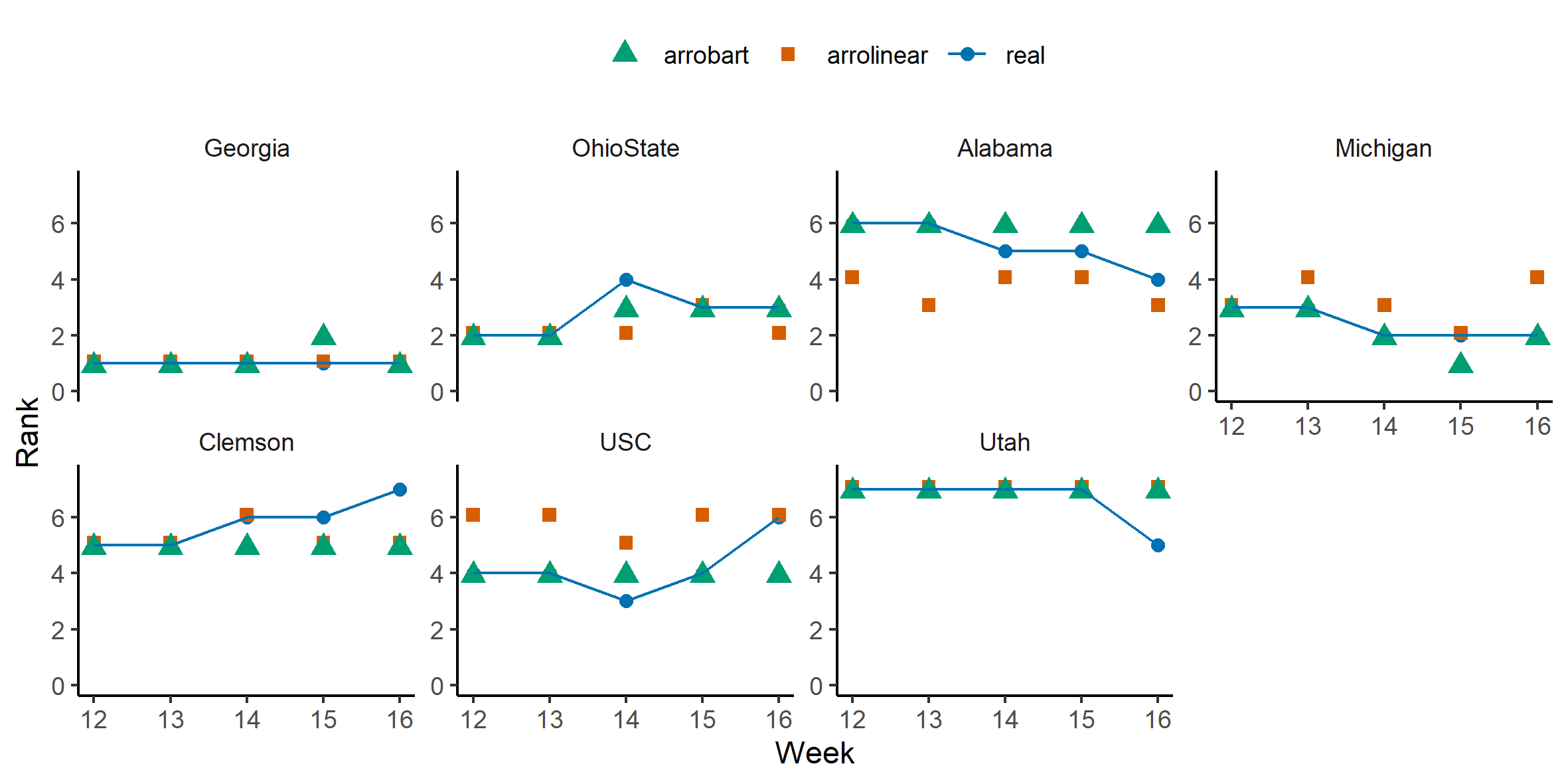
Figure 2: AP Pollster Brian Howell: observed poll ranks (blue dots and line) and ranks forecasted using the ARROBART (green triangles) and ARROLinear (orange squares) models.

To inspect in more detail the advantages of the BART specification compared to the linear one, we report the point forecasts from the best ARROBART and ARROLinear models in Fig. 2 against the observed ranks, for $N=7$ teams and $h=5$ test periods. As the rankers are assumed to be independent, we present the results for a single pollster. The ARROBART model is able to correctly predict the rank for several teams, with minor deviations for Alabama and Clemson. Conversely, the ARROLinear forecasts are generally more distant from the actual ranks. In particular, it can be observed that while both methods often produce similar forecasts, ARROBART produces more accurate forecasts for Alabama, USC, and Michigan in weeks 12 to 14.

The point forecast falls short of quantifying the uncertainty about the predicted value. To tackle this issue, we investigate in deeper detail the posterior predictive distribution of the best-performing model. Figure 3 reports the posterior predictive distribution of the rank for Alabama and Michigan, whose observed ranks have changed multiple times during the testing sample (see Fig. 2). For both teams, the predictive density of the rank is unimodal and changes over time in terms of its mode and dispersion, suggesting a horizon-specific uncertainty of predictions. Furthermore, the comparison of Fig. 2 and Fig. 3 highlights that in those periods where the point forecast differs from the observed one, the latter falls within the second-most frequent rank of the posterior predictive distribution.

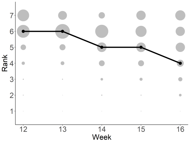
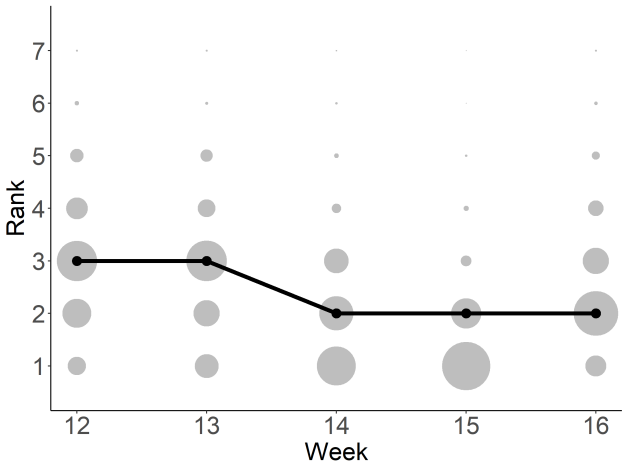
Figure 3: ARROBART posterior predictive distribution (grey balls, with size proportional to the probability mass) against the observed ranks (black dots and line) for Alabama (left) and Michigan (right) ranks of AP Pollster Brian Howell.

6 Discussion

This article introduces a novel class of nonparametric Thurstone models for static and dynamic regressions for rank-order data called ROBART and ARROBART. The proposed frameworks use a BART specification for the regression function of the latent variable representation to allow for flexible, possibly nonlinear relationships between the latent scores and their lagged values as well as exogenous covariates. The filtering and smoothing recursions for the dynamic model are derived, followed by a discussion on the computational tools needed to sample from them. A simulation study illustrates that the proposed ROBART and ARROBART outperform the competitors in a forecasting setting. The ARROBART model is applied to an out-of-sample forecasting exercise of a real dataset of weekly rankings of American football teams for the 2022 NCAA season. The results highlight the better performance of the ARROBART family compared to linear and static counterparts. Overall, this suggests the importance of accounting for temporal persistence in sports rankings and the usefulness of BART in accounting for the nonlinearities driving the evolution of the latent team-specific scores.

Besides representing an advancement in the literature on rank-order data and time series of them, the proposed methods can be applied to a wide range of datasets other than sports data. Examples include the analysis of the main drivers of customers’ rankings, university rankings, and political ratings. In the presence of more complex dynamics of the latent scores, the proposed ARROBART model can be generalised to $p>1$ lags. Other interesting possible extensions of the proposed methods include investigating the performance of more general BART specifications. For instance, the introduction of a varying-coefficient BART (Deshpande et al., 2022) or of the Dirichlet additive regression trees approach (Linero and Yang, 2018), which assumes a Dirichlet hyperprior for the BART variable splitting probabilities. These methods would allow us to alleviate or address the main shortcomings of plain BART specifications, such as their lack of smoothness and vulnerability to the curse of dimensionality. The proposed autoregressive BART methods can also be adapted to investigate binary outcome data and count data, which are popular for example in epidemiology and climate studies. These data are characterized by potentially highly nonlinear dynamics and/or relationships with external factors, thus making the use of BART a viable candidate for improving forecasting performance. Finally, it would be interesting to extend the proposed dynamic model to investigate the problem of aggregation of ranking lists (Deng et al., 2014; Zhu et al., 2023) in a time series setting.

Supplementary Materials

An online Supplement provides proof of the results, the derivation of the posterior, details on the simulation study, and additional results for the application to NCAA football data.

References

- Alvo and Philip (2014) Alvo, M. and L. Philip (2014). Statistical methods for ranking data, Volume 1341. Springer.
- Bradlow and Fader (2001) Bradlow, E. T. and P. S. Fader (2001). A Bayesian lifetime model for the “Hot 100” Billboard songs. Journal of the American Statistical Association 96(454), 368–381.
- Cappé et al. (2005) Cappé, O., E. Moulines, and T. Rydén (2005). Inference in hidden Markov models. Springer.
- Chipman et al. (2010) Chipman, H. A., E. I. George, and R. E. McCulloch (2010). BART: Bayesian additive regression trees. The Annals of Applied Statistics 4(1), 266–298.
- Deng et al. (2014) Deng, K., S. Han, K. J. Li, and J. S. Liu (2014). Bayesian aggregation of order-based rank data. Journal of the American Statistical Association 109(507), 1023–1039.
- Deshpande et al. (2022) Deshpande, S. K., R. Bai, C. Balocchi, J. E. Starling, and J. Weiss (2022). VCBART: Bayesian trees for varying coefficients. arXiv:2003.06416.
- Dwork et al. (2001) Dwork, C., R. Kumar, M. Naor, and D. Sivakumar (2001). Rank aggregation methods for the web. In Proceedings of the 10th international conference on World Wide Web, pp. 613–622.
- Fok et al. (2012) Fok, D., R. Paap, and B. Van Dijk (2012). A rank-ordered logit model with unobserved heterogeneity in ranking capabilities. Journal of Applied Econometrics 27(5), 831–846.
- Glickman and Hennessy (2015) Glickman, M. E. and J. Hennessy (2015). A stochastic rank ordered logit model for rating multi-competitor games and sports. Journal of Quantitative Analysis in Sports 11(3), 131–144.
- Gormley and Murphy (2008) Gormley, I. C. and T. B. Murphy (2008). Exploring voting blocs within the Irish electorate: A mixture modeling approach. Journal of the American Statistical Association 103(483), 1014–1027.
- Graves et al. (2003) Graves, T., C. S. Reese, and M. Fitzgerald (2003). Hierarchical models for permutations: Analysis of auto racing results. Journal of the American Statistical Association 98(462), 282–291.
- Grewal et al. (2008) Grewal, R., J. A. Dearden, and G. L. Llilien (2008). The university rankings game: Modeling the competition among universities for ranking. The American Statistician 62(3), 232–237.
- Gu and Yu (2023) Gu, J. and P. L. Yu (2023). Social order statistics models for ranking data with analysis of preferences in social networks. The Annals of Applied Statistics 17(1), 89–107.
- Henderson and Kirrane (2018) Henderson, D. A. and L. J. Kirrane (2018). A comparison of truncated and time-weighted Plackett–Luce models for probabilistic forecasting of Formula One results. Bayesian Analysis 13(2), 335–358.
- Hill et al. (2020) Hill, J., A. Linero, and J. Murray (2020). Bayesian additive regression trees: A review and look forward. Annual Review of Statistics and its Application 7, 251–278.
- Hoff (2009) Hoff, P. D. (2009). A first course in Bayesian statistical methods, Volume 580. Springer.
- Huber et al. (2023) Huber, F., G. Koop, L. Onorante, M. Pfarrhofer, and J. Schreiner (2023). Nowcasting in a pandemic using non-parametric mixed frequency VARs. Journal of Econometrics 232(1), 52–69.
- Huber and Rossini (2022) Huber, F. and L. Rossini (2022). Inference in Bayesian additive vector autoregressive tree models. Annnals of Applied Statistics 16(1), 104–123.
- Johnson et al. (2002) Johnson, V. E., R. O. Deaner, and C. P. Van Schaik (2002). Bayesian analysis of rank data with application to primate intelligence experiments. Journal of the American Statistical Association 97(457), 8–17.
- Kendall (1938) Kendall, M. G. (1938). A new measure of rank correlation. Biometrika 30(1/2), 81–93.
- Li et al. (2022) Li, X., D. Yi, and J. S. Liu (2022). Bayesian analysis of rank data with covariates and heterogeneous rankers. Statistical Science 37(1), 1–23.
- Lin and Ding (2009) Lin, S. and J. Ding (2009). Integration of ranked lists via cross entropy Monte Carlo with applications to mRNA and microRNA studies. Biometrics 65(1), 9–18.
- Linero and Yang (2018) Linero, A. R. and Y. Yang (2018). Bayesian regression tree ensembles that adapt to smoothness and sparsity. Journal of the Royal Statistical Society: Series B (Statistical Methodology) 80(5), 1087–1110.
- Liu et al. (2019) Liu, Q., M. Crispino, I. Scheel, V. Vitelli, and A. Frigessi (2019). Model-based learning from preference data. Annual Review of Statistics and its Application 6, 329–354.
- Luce (1959) Luce, R. D. (1959). Individual choice behavior. New York: Wiley.
- Plackett (1975) Plackett, R. L. (1975). The analysis of permutations. Journal of the Royal Statistical Society: Series C (Applied Statistics) 24(2), 193–202.
- Thurstone (1927) Thurstone, L. L. (1927). A law of comparative judgment. Psychological review 34(4), 273.
- Walker and Ben-Akiva (2002) Walker, J. and M. Ben-Akiva (2002). Generalized random utility model. Mathematical Social Sciences 43(3), 303–343.
- Yu (2000) Yu, P. L. (2000). Bayesian analysis of order-statistics models for ranking data. Psychometrika 65(3), 281–299.
- Zhu et al. (2023) Zhu, W., Y. Jiang, J. S. Liu, and K. Deng (2023). Partition–mallows model and its inference for rank aggregation. Journal of the American Statistical Association 118(541), 343–359.