Machine Learning-powered Combinatorial Clock Auction

Abstract

We study the design of iterative combinatorial auctions (ICAs). The main challenge in this domain is that the bundle space grows exponentially in the number of items. To address this, several papers have recently proposed machine learning (ML)-based preference elicitation algorithms that aim to elicit only the most important information from bidders. However, from a practical point of view, the main shortcoming of this prior work is that those designs elicit bidders’ preferences via value queries (i.e., “What is your value for the bundle $\{A,B\}$?”). In most real-world ICA domains, value queries are considered impractical, since they impose an unrealistically high cognitive burden on bidders, which is why they are not used in practice. In this paper, we address this shortcoming by designing an ML-powered combinatorial clock auction that elicits information from the bidders only via demand queries (i.e., “At prices $p$, what is your most preferred bundle of items?”). We make two key technical contributions: First, we present a novel method for training an ML model on demand queries. Second, based on those trained ML models, we introduce an efficient method for determining the demand query with the highest clearing potential, for which we also provide a theoretical foundation. We experimentally evaluate our ML-based demand query mechanism in several spectrum auction domains and compare it against the most established real-world ICA: the combinatorial clock auction (CCA). Our mechanism significantly outperforms the CCA in terms of efficiency in all domains, it achieves higher efficiency in a significantly reduced number of rounds, and, using linear prices, it exhibits vastly higher clearing potential. Thus, with this paper we bridge the gap between research and practice and propose the first practical ML-powered ICA.

1 Introduction

Combinatorial auctions (CAs) are used to allocate multiple items among several bidders who may view those items as complements or substitutes. In a CA, bidders are allowed to submit bids over bundles of items. CAs have enjoyed widespread adoption in practice, with their applications ranging from allocating spectrum licences (Cramton 2013) to TV ad slots (Goetzendorff et al. 2015) and airport landing/take-off slots (Rassenti, Smith, and Bulfin 1982).

One of the key challenges in CAs is that the bundle space grows exponentially in the number of items, making it infeasible for bidders to report their full value function in all but the smallest domains. Moreover, Nisan and Segal (2006) showed that for general value functions, CAs require an exponential number of bids in order to achieve full efficiency in the worst case. Thus, practical CA designs cannot provide efficiency guarantees in real world settings with more than a modest number of items. Instead, the focus has shifted towards iterative combinatorial auctions (ICAs), where bidders interact with the auctioneer over a series of rounds, providing a limited amount of information, and the aim of the auctioneer is to find a highly efficient allocation.

The most established mechanism following this interaction paradigm is the combinatorial clock auction (CCA) (Ausubel, Cramton, and Milgrom 2006). The CCA has been used extensively for spectrum allocation, generating over $\$20$ Billion in revenue between $2012$ and $2014$ alone (Ausubel and Baranov 2017). Speed of convergence is a critical consideration for any ICA since each round can entail costly computations and business modelling for the bidders (Kwasnica et al. 2005; Milgrom and Segal 2017; Bichler, Hao, and Adomavicius 2017). Large spectrum auctions following the CCA format can take more than $100$ bidding rounds. In order to decrease the number of rounds, many CAs in practice use aggressive price update rules (e.g., increasing prices by up to $10$% each round), which can harm efficiency (Ausubel and Baranov 2017). Thus, it remains a challenging problem to design a practical ICA that elicits information via demand queries, is efficient, and converges in a small number of rounds. Specifically, given the value of resources allocated in such real-world ICAs, increasing their efficiency by even one percentage point already translates into monetary gains of hundreds of millions of dollars.

1.1 ML-Powered Preference Elicitation

To address this challenge, researchers have proposed various ways of using machine learning (ML) to improve the efficiency of CAs. The seminal works by Blum et al. (2004) and Lahaie and Parkes (2004) were the first to frame preference elicitation in CAs as a learning problem. In the same strand of research, Brero, Lubin, and Seuken (2018, 2021), Weissteiner and Seuken (2020) and Weissteiner et al. (2022b) proposed ML-powered ICAs. At the heart of those approaches lies an ML-powered preference elicitation algorithm that uses an ML model to approximate each bidder’s value function and to generate the next value query, which in turn refines that bidder’s model. Weissteiner et al. (2022a) designed a special network architecture for this framework while Weissteiner et al. (2023) incorporated a notion of uncertainty (Heiss et al. 2022) into the framework, further increasing its efficiency. Despite their great efficiency gains compared to traditional CA designs, those approaches suffer from one common limitation. They fundamentally rely on value queries of the form “What is your value for bundle $\{A,B\}$”, which are cognitively more complex, and thus typically impractical for real-world ICAs that instead prioritize employing demand queries.

Conceptually, most related to the present paper is the work by Brero and Lahaie (2018) and Brero, Lahaie, and Seuken (2019), who proposed integrating ML in a price-based ICA to generate the next price vector in order to achieve faster convergence. Similar to our design, in these works the auctioneer maintains a model of each agent’s value function, which are updated as the agents bid in the auction and reveal more information about their values. Then, those models are used in each round to compute new prices and drive the bidding process. Unlike our approach, the design of this prior work focuses only on clearing potential, as the authors do not report efficiency results. Additionally, their design suffers from some significant limitations: (i) it does not exploit any notion of similarity between bundles that contain overlapping items, (ii) it only incorporates a small part of the information revealed by the agents’ bidding. Specifically, they only make use of the fact that for the bundle an agent bids on, her value for it must be larger than its price, and (iii) their approach is computationally intractable already in medium-sized auction domains, as their price update rule requires a large number $l$ of posterior samples for expectation maximization and then solving a linear program whose number of constraints for each bidder is proportional to $l$ times the number of bids by that agent. These limitations are significant, as they can lead to large efficiency decreases in complex combinatorial domains. Furthermore, their design cannot be easily modified to alleviate these limitations.

1.2 Our Contributions

In this paper, we address the main shortcomings of prior work by designing an ML-powered combinatorial clock auction. Our auction elicits information from bidders via demand queries instead of value queries, while simultaneously being computationally feasible for large domains and incorporating the complete information the demand query observations provide into the training of our ML models. Concretely, we use Monotone-Value Neural Networks (MVNNs) (Weissteiner et al. 2022a) as ML models, which are tailored to model monotone and non-linear combinatorial value functions in CAs.

The main two technical challenges are (i) training those MVNNs only on demand query observations and (ii) efficiently determining the next demand query that is most likely to clear the market based on the trained MVNNs. In detail, we make the following contributions:

1. We first propose an adjusted MVNN architecture, which we call multiset MVNNs (mMVNNs). mMVNNs can be used more generally in multiset domains (i.e., if multiple indistinguishable copies of the same good exist) (Section 3.1) and we prove the universality property of mMVNNs in such multiset domains (Theorem 1).

2. We present a novel method for training mMVNNs on demand query observations (Section 3.2).

3. We introduce an efficient method for determining the price vector that is most likely to clear the market based on the trained ML models (Section 4). For this, we derive a simple and intuitive price update rule that results from performing GD on an objective function which is minimized exactly at clearing prices (Theorem 3).

4. Based on Items 2 and 3, we propose a practical ML-powered clock auction (Section 5).

5. We experimentally show that compared to the CCA, our ML-powered clock auction can achieve substantially higher efficiency on the order of 9% points. Furthermore, using linear prices, our ML-powered clock auction exhibits significantly higher clearing potential compared to the CCA (Section 6).

GitHub

Our source code is publicly available on GitHub via: https://github.com/marketdesignresearch/ML-CCA.

1.3 Further Related Work

In the field of automated mechanism design, Dütting et al. (2015, 2019), Golowich, Narasimhan, and Parkes (2018) and Narasimhan, Agarwal, and Parkes (2016) used ML to learn new mechanisms from data, while Cole and Roughgarden (2014); Morgenstern and Roughgarden (2015) and Balcan, Sandholm, and Vitercik (2023) bounded the sample complexity of learning approximately optimal mechanisms. In contrast to this prior work, our design incorporates an ML algorithm into the mechanism itself, i.e., the ML algorithm is part of the mechanism. Lahaie and Lubin (2019) suggest an adaptive price update rule that increases price expressivity as the rounds progress in order to improve efficiency and speed of convergence. Unlike that work, we aim to improve preference elicitation while still using linear prices. Preference elicitation is a key market design challenge outside of CAs too. Soumalias et al. (2023) introduce an ML-powered mechanism for course allocation that improves preference elicitation by asking students comparison queries.

1.4 Practical Considerations and Incentives

Our ML-powered clock phase can be viewed as an alternative to the clock phase of the CCA. In a real-world application, many other considerations (beyond the price update rule) are also important. For example, the careful design of activity rules is vital to induce truthful bidding in the clock phase of the CCA (Ausubel and Baranov 2017). The payment rule used in the supplementary round is also important, and it has been argued that the use of the VCG-nearest payment rule, while not strategy-proof, induces good incentives in practice (Cramton 2013). Similar to the clock phase of the CCA, our ML-powered clock phase is not strategyproof. If our design were to be fielded in a real-world environment, we envision that one would combine it with carefully designed activity and payment rules in order to induce good incentives. Thus, we consider the incentive problem orthogonal to the price update problem and in the rest of the paper, we follow prior work (Brero, Lahaie, and Seuken 2019; Parkes and Ungar 2000) and assume that bidders follow myopic best-response (truthful) bidding throughout all auction mechanisms tested.

2 Preliminaries

2.1 Formal Model for ICAs

We consider multiset CA domains with a set $N=\{1,\ldots,n\}$ of bidders and a set $M=\{1,\ldots,m\}$ of distinct items with corresponding capacities, i.e., number of available copies, $c=(c_{1},\ldots,c_{m})\in\mathbb{N}^{m}$. We denote by $x\in\mathcal{X}=\{0,\ldots,c_{1}\}\times\ldots\times\{0,\ldots c_{m}\}$ a bundle of items represented as a positive integer vector, where $x_{j}=k$ iff item $j\in M$ is contained $k$-times in $x$. The bidders’ true preferences over bundles are represented by their (private) value functions $v_{i}:\mathcal{X}\to\mathbb{R}_{\geq 0},\,\,i\in N$, i.e., $v_{i}(x)$ represents bidder $i$’s true value for bundle $x\in\mathcal{X}$. We collect the value functions $v_{i}$ in the vector $v=(v_{i})_{i\in N}$. By $a=(a_{1},\ldots,a_{n})\in\mathcal{X}^{n}$ we denote an allocation of bundles to bidders, where $a_{i}$ is the bundle bidder $i$ obtains. We denote the set of feasible allocations by $\mathcal{F}=\left\{a\in\mathcal{X}^{n}:\sum_{i\in N}a_{ij}\leq c_{j},\,\,\forall j\in M\right\}$. We assume that bidders have quasilinear utility functions $u_{i}$ of the form $u_{i}(a_{i})=v_{i}(a_{i})-\pi_{i}$ where $v_{i}$ can be highly non-linear and $\pi_{i}\in\mathbb{R}_{\geq 0}$ denotes the bidder’s payment. This implies that the (true) social welfare $V(a)$ of an allocation $a$ is equal to the sum of all bidders’ values $\sum_{i\in N}v_{i}(a_{i})$. We let $a^{*}\in\operatorname*{argmax}_{a\in{\mathcal{F}}}V(a)$ denote a social-welfare maximizing, i.e., efficient, allocation. The efficiency of any allocation $a\in\mathcal{F}$ is determined as $V(a)/V(a^{*})$.

An ICA mechanism defines how the bidders interact with the auctioneer and how the allocation and payments are determined. In this paper, we consider ICAs that iteratively ask bidders linear demand queries. In such a query, the auctioneer presents a vector of item prices $p\in\mathbb{R}^{m}_{\geq 0}$ and each bidder $i$ responds with her utility-maximizing bundle, i.e.,

$$x_{i}^{*}(p)\in\operatorname*{argmax}_{x\in\mathcal{X}}\left\{v_{i}(x)-\left\langle p,x\right\rangle\right\}\,i\in N,$$ (1)

where $\left\langle\cdot,\cdot\right\rangle$ denotes the Euclidean scalar product in $\mathbb{R}^{m}$.

Even though our approach could conceptually incorporate any kind of (non-linear) price function $p:\mathcal{X}\to\mathbb{R}_{\geq 0}$, our concrete implementation will only use linear prices (i.e., prices over items). Linear prices are most established in practice since they are intuitive and simple for the bidders to understand (e.g., (Ausubel, Cramton, and Milgrom 2006)).

For bidder $i\in N$, we denote a set of $K\in\mathbb{N}$ such elicited utility-maximizing bundles and price pairs as $R_{i}=\left\{\left(x_{i}^{*}(p^{r}),p^{r}\right)\right\}_{r=1}^{K}$. Let $R=(R_{1},\ldots,R_{n})$ be the tuple of elicited demand query data from all bidders. The ICA’s (inferred) optimal feasible allocation $a^{*}(R)\in\mathcal{F}$ and payments $\pi_{i}\coloneqq\pi_{i}(R)\in\mathbb{R}^{n}_{+}$ are computed based on the elicited reports $R$ only. Concretely, $a^{*}_{R}\in\mathcal{F}$ is defined as

$$a^{*}(R)\in\operatorname*{argmax}_{\begin{subarray}{c}\mathcal{F}\,\ni\,\left(x_{i}^{*}\left(p^{r_{i}}\right)\right)_{i=1}^{n}\\ :\,r_{i}\in\{1,\ldots,K\}\,\forall i\in N\end{subarray}}\sum_{i\in N}\left\langle p^{r_{i}},x_{i}^{*}(p^{r_{i}})\right\rangle.$$ (2)

As payment rule $\pi_{i}(R)$ one could use any reasonable choice (e.g., VCG payments, see Appendix A). As the auctioneer can only ask a limited number of demand queries $|R_{i}|\leq Q^{\textrm{max}}$ (e.g., $Q^{\textrm{max}}=100$), an ICA needs a practically feasible and smart preference elicitation algorithm.

2.2 The Combinatorial Clock Auction (CCA)

We consider the CCA (Ausubel, Cramton, and Milgrom 2006) as the main benchmark auction. The CCA consists of two phases. The initial clock phase proceeds in rounds. In each round, the auctioneer presents anonymous item prices $p\in\mathbb{R}_{\geq 0}^{m}$, and each bidder is asked to respond to a demand query, declaring her utility-maximizing bundle at $p$. The clock phase of the CCA is parametrized by the reserve prices employed in its first round, and the way prices are updated. An item $j$ is over-demanded at prices $p$, if, for those prices, its total demand based on the bidders’ responses to the demand query exceeds its capacity, i.e., $\sum_{i\in N}(x_{i}^{*}(p))_{j}>c_{j}$. The most common price update rule is to increase the price of all over-demanded items by a fixed percentage, which we set to $5\%$ for our experiments, as in many real-world applications (e.g., (Industry Canada 2013)).

The second phase of the CCA is the supplementary round. In this phase, each bidder can submit a finite number of additional bids for bundles of items, which are called push bids. Then, the final allocation is determined based on the combined set of all inferred bids of the clock phase, plus all submitted push bids of the supplementary round. This design aims to combine good price discovery in the clock phase with good expressiveness in the supplementary round. In simulations, the supplementary round is parametrized by the assumed bidder behaviour in this phase, i.e., which bundle-value pairs they choose to report. As in (Brero, Lubin, and Seuken 2021), we consider the following heuristics when simulating bidder behaviour:

• Clock Bids: Corresponds to having no supplementary round. Thus, the final allocation is determined based only on the inferred bids of the clock phase (Equation 2).

• Raised Clock Bids: The bidders also provide their true value for all bundles they bid on during the clock phase.

• Profit Max: Bidders provide their true value for all bundles that they bid on in the clock phase, and additionally submit their true value for the $Q^{\textrm{P-Max}}$ bundles earning them the highest utility at the prices of the final clock phase.

3 Training on Demand Query Observations

In this section, we first propose a new version of MVNNs that are applicable to multiset domains $\mathcal{X}$ and extend the universality proof of classical MVNNs. Finally, we present our demand-query training algorithm.

Input : Demand query data $R_{i}=\left\{\left(x_{i}^{*}(p^{r}),p^{r}\right)\right\}_{r=1}^{K}$, Epochs $T\in\mathbb{N}$, Learning Rate $\gamma>0$.

1 $\theta_{0}\leftarrow$ init mMVNN $\triangleright$ Weissteiner et al. (2023, S.3.2)

2 for $t=0\text{ to }T-1$ do

3       for $r=1\text{ to }K$ do $\triangleright$ Demand responses for prices

4             Solve $\hat{x}^{*}_{i}(p^{r})\in\operatorname*{argmax}_{x\in\mathcal{X}}\mathcal{M}_{i}^{\theta_{t}}(x)-\left\langle p^{r},x\right\rangle$

5             if $\hat{x}^{*}_{i}(p^{r})\neq x_{i}^{*}(p^{r})$ then $\triangleright$ mMVNN is wrong

                   $L(\theta_{t})\leftarrow(\mathcal{M}_{i}^{\theta_{t}}(\hat{x}^{*}_{i}(p^{r}))-\left\langle p^{r},\hat{x}^{*}_{i}(p^{r})\right\rangle)-(\mathcal{M}_{i}^{\theta_{t}}(x_{i}^{*}(p^{r}))-\left\langle p^{r},x_{i}^{*}(p^{r})\right\rangle)$

                    $\triangleright$ Add predicted utility difference to loss

                   $\theta_{t+1}\leftarrow\theta_{t}-\gamma(\nabla_{\theta}L(\theta))_{\theta=\theta_{t}}$

                    $\triangleright$ SGD step

6                  

return Trained parameters $\theta_{T}$ of the mMVNN $\mathcal{M}_{i}^{\theta_{T}}$

Algorithm 1 TrainOnDQs

3.1 Multiset MVNNs

MVNNs (Weissteiner et al. 2022a) are a recently introduced class of NNs specifically designed to represent monotone combinatorial valuations. In the following, we present an adapted version of the MVNNs, which we call multiset MVNNs (mMVNNs). For mMVNNs, we add a linear normalization layer D after the input layer. We add this normalization since the input (i.e., a bundle) $x\in\mathcal{X}$ is a positive integer vector instead of a binary vector as in the classic case of indivisible items with capacities $c_{j}=1$ for all $j\in M$. This normalization ensures that $\hyperref@@ii[itm:D]{\normalcolor D}x\in[0,1]$ and thus we can use the weight initialization scheme from (Weissteiner et al. 2023). For details, please see Appendix B.

Definition 1 (Multiset MVNN).

An mMVNN $\mathcal{M}_{i}^{\theta}:\mathcal{X}\to\mathbb{R}_{\geq 0}$ for bidder $i\in N$ is defined as

$$\mathcal{M}_{i}^{\theta}(x)\coloneqq W^{i,K_{i}}\varphi_{0,t^{i,K_{i}-1}}\left(\ldots\varphi_{0,t^{i,1}}(W^{i,1}\left(\hyperref@@ii[itm:D]{\normalcolor D}x\right)+b^{i,1})\ldots\right)$$ (3)

• $K_{i}+2\in\mathbb{N}$ is the number of layers ($K_{i}$ hidden layers),

• $\{\varphi_{0,t^{i,k}}{}\}_{k=1}^{K_{i}-1}$ are the MVNN-specific activation functions with cutoff $t^{i,k}>0$, called bounded ReLU (bReLU):

  $$\varphi_{0,t^{i,k}}(\cdot)\coloneqq\min(t^{i,k},\max(0,\cdot))$$ (4)

• $W^{i}\coloneqq(W^{i,k})_{k=1}^{K_{i}}$ with $W^{i,k}\geq 0$ and $b^{i}\coloneqq(b^{i,k})_{k=1}^{K_{i}-1}$ with $b^{i,k}\leq 0$ are the non-negative weights and non-positive biases of dimensions $d^{i,k}\times d^{i,k-1}$ and $d^{i,k}$, whose parameters are stored in $\theta=(W^{i},b^{i})$.

• $\hyperref@@ii[itm:D]{\normalcolor D}\coloneqq\operatorname{diag}\left(\nicefrac{{1}}{{c_{1}}},\ldots,\nicefrac{{1}}{{c_{m}}}\right)$ is the linear normalization layer that ensures $\hyperref@@ii[itm:D]{\normalcolor D}x\in[0,1]$ and is not trainable.

In Theorem 1, we extend the proof from Weissteiner et al. (2022a) and show that mMVNNs are also universal in the set of monotone value functions defined on a multiset domain $\mathcal{X}$. For this, we first define the following properties:

1. Monotonicity (“more items weakly increase value”):
   For $a,b\in\mathcal{X}$: if $a\leq b$, i.e. $\forall k\in M:a_{i}\leq b_{i}$, it holds that $v_{i}(a)\leq v_{i}(b)$,

2. Normalization (”no value for empty bundle”):
   $v_{i}(\emptyset)=v_{i}((0,\ldots,0))\coloneqq 0$,

These properties are common assumptions and are satisfied in many market domains. We can now present the following universality result:

Theorem 1 (Multiset Universality).

Any value function $v_{i}:\mathcal{X}\to\mathbb{R}_{+}$ that satisfies (M) and (N) can be represented exactly as an mMVNN $\mathcal{M}_{i}^{\theta}$ from Definition 1, i.e., for $\mathcal{V}:=\{v_{i}:\mathcal{X}\to\mathbb{R}_{+}|\,\text{satisfy {(M)} and {(N)}}\}$ it holds that

$$\mathcal{V}=\left\{\mathcal{M}_{i}^{(W^{i},b^{i})}:W^{i}\geq 0,b^{i}\leq 0\}\right\}.$$ (5)

Proof.

Please, see Section B.2 for the proof. ∎

Furthermore, we can formulate maximization over mMVNNs, i.e., $\max_{x\in\mathcal{X}}\mathcal{M}_{i}^{\theta}(x)-\left\langle p,x\right\rangle$, as a mixed integer linear program (MILP) analogously to Weissteiner et al. (2022a), which will be key for our ML-powered clock phase.

3.2 Training Algorithm

In Algorithm 1, we describe how we train, for each bidder $i\in N$, a distinct mMVNN $\mathcal{M}_{i}^{\theta}$ on demand query data $R_{i}$.

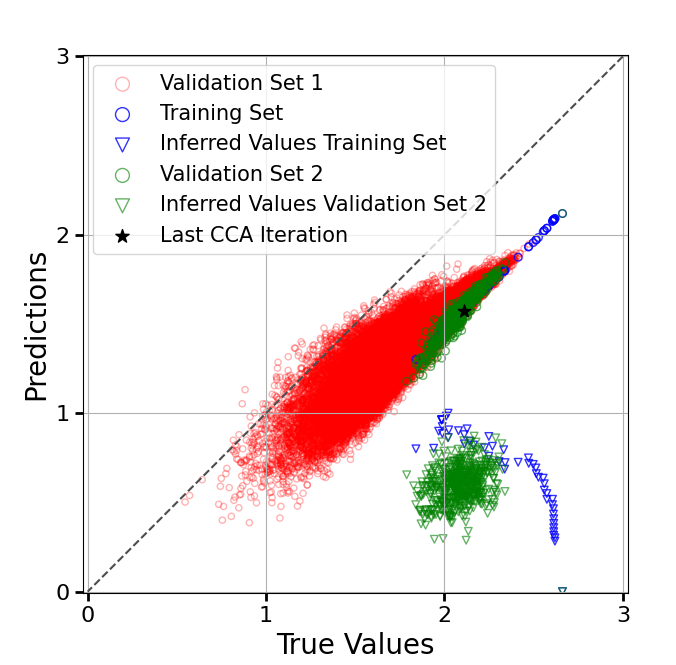
Figure 1: Scaled prediction vs. true plot of a trained mMVNN via Algorithm 1 for the national bidder in the MRVM domain (see Section 6).

Our design choices regarding this training algorithm are motivated by the information that responses to demand queries provide. According to myopic best response bidding, at each round $r$, bidder $i$ reports a utility-maximizing bundle $x_{i}^{*}\left(p^{r}\right)\in\mathcal{X}$ at current prices $p^{r}$. Formally, for all $x\in\mathcal{X}$:

$$v_{i}(x_{i}^{*}\left(p^{r}\right))-\left\langle p^{r},x_{i}^{*}\left(p^{r}\right)\right\rangle\geq v_{i}(x)-\left\langle p^{r},x\right\rangle.$$ (6)

Notice that for any epoch $t$ and round $r$, the loss $L(\theta_{t})$ for that round calculated in Algorithms 1, 1 and 1 is always non-negative, and can only be zero if the mMVNN $\mathcal{M}_{i}^{\theta}$ (instead of $v_{i}$) satisfies Equation 6. Thus, the loss for an epoch is zero iff the mMVNN $\mathcal{M}_{i}^{\theta}$ satisfies Equation 6 for all rounds, and in that case the model has captured the full information provided by the demand query responses $R_{i}$ of that bidder. Finally, note that Algorithm 1 can be applied to any MILP-formalizable ML model whose parameters can be efficiently updated via GD, such as MVNNs or ReLU-NNs.

In Figure 1, we present a prediction vs. true plot of an mMVNN, which we trained via Algorithm 1. We present the training set of $50$ demand query data points $R_{i}$ in blue circles, where the prices $\{p^{r}\}_{r=1}^{50}$ are generated according to the same rule as in CCA. Additionally, we mark the bundle $x^{\text{CCA}}\in\mathcal{X}$ from this last CCA iteration (i.e., the one resulting from $p^{50}$) with a black star. Moreover, we present two different validation sets on which we evaluate mMVNN configurations in our hyperparameter optimization (HPO): Validation set 1 (red circles), which are $50,000$ uniformly at random sampled bundles $x\in\mathcal{X}$, and validation set 2 (green circles), where we first sample $500$ price vectors $\{p^{r}\}_{r=1}^{500}$ where the price of each item is drawn uniformly at random from the range of $0$ to $3$ times the average maximum value of an agent of that type for a single item, and then determine utility-maximizing bundles $x_{i}^{*}(p^{r})$ (w.r.t. $v_{i}$) at those prices (cp. Equation 1). While validation set 1 measures generalization performance in a classic sense over the whole bundle space, validation set 2 focuses on utility-maximizing bundles. We additionally demonstrate the inferred values of the bundles of the training set and validation set 2 using triangles of the same colour, i.e., $\{\left\langle p^{r},x_{i}^{*}(p^{r})\right\rangle\}_{r=1}^{50/500}$. These triangles highlight the only cardinal information that our mMVNNs have access to during training and are a lower bound of the true value. In Figure 1, we see that our mMVNN is able to learn at the training points (blue circles) the true value functions almost perfectly up to a constant shift $\kappa$, i.e., $\mathcal{M}_{i}^{\theta_{T}}(x)\approx v_{i}(x)+\kappa$. This is true even though the corresponding inferred values (blue triangles) are very far off from the true values $\left\langle p^{r},x_{i}^{*}(p^{r})\right\rangle\ll v_{i}(x_{i}^{*}(p^{r}))$. Moreover, the mMVNN generalizes well (up to the constant shift $\kappa$) on validation sets 1 and 2. Overall, this shows that Algorithm 1 indeed leads to mMVNNs $\mathcal{M}_{i}^{\theta_{T}}$ which are a good approximation of $v_{i}+\kappa$. Note that learning the true value function up to a constant shift suffices for our proposed demand query generation procedure presented in Section 4.

4 ML-powered Demand Query Generation

In this section, we show how we generate ML-powered demand queries and provide the theoretical foundation for our approach by extending a well-known connection between clearing prices, efficiency and a clearing objective function. First, we define indirect utility, revenue and clearing prices.

Definition 2 (Indirect Utility and Revenue).

For linear prices $p\in\mathbb{R}_{\geq 0}^{m}$, a bidder’s indirect utility $U$ and the seller’s indirect revenue $R$ are defined as

$$U(p,v_{i})\coloneqq\max\limits_{x\in\mathcal{X}}\left\{v_{i}(x)-\left\langle p,x\right\rangle\right\}\text{ and }$$ (7)

$$R(p)\coloneqq\max\limits_{a\in\mathcal{F}}\left\{\sum\limits_{i\in N}\left\langle p,a_{i}\right\rangle\right\}\stackrel{{\scriptstyle\hyperref@@ii[foot:Rlinear]{}}}{{\hyperlink{proof:app:eq:indirect_revenue}{=}}}\sum\limits_{j\in M}c_{j}p_{j},$$ (8)

i.e., at prices $p$, Equations 7 and 8 are the maximum utility a bidder can achieve for all $x\in\mathcal{X}$ and the maximum revenue the seller can achieve among all feasible allocations.

Definition 3 (Clearing Prices).

Prices $p\in\mathbb{R}_{\geq 0}^{m}$ are clearing prices if there exists an allocation $a(p)\in\mathcal{F}$ such that

1. for each bidder $i$, the bundle $a_{i}(p)$ maximizes her utility, i.e., $v_{i}(a_{i}(p))-\left\langle p,a_{i}(p)\right\rangle=U(p,v_{i}),\forall i\in N$, and

2. the allocation $a(p)\in\mathcal{F}$ maximizes the sellers revenue, i.e., $\sum_{i\in N}\left\langle p,a_{i}(p)\right\rangle=R(p)$.

Next, we provide an important connection between clearing prices, efficiency and a clearing objective $W$. Theorem 2 extends Bikhchandani and Ostroy (2002, Theorem 3.1).

Theorem 2.

Consider the notation from Definitions 2 and 3 and the objective function $W(p,v)\coloneqq R(p)+\sum_{i\in N}U(p,v_{i})$. Then it holds that, if a linear clearing price vector exists, every price vector

$$p^{\prime}\in \operatorname*{argmin}_{\tilde{p}\in\mathbb{R}_{\geq 0}^{m}} W(\tilde{p},v)$$ (9a)

such that $$(x^{*}_{i}(\tilde{p}))_{i\in N}\in\mathcal{F}$$ (9b)

is a clearing price vector and the corresponding allocation $a(p^{\prime})\in\mathcal{F}$ is efficient.

Proof.

We provide the proof in Section C.1. ∎

Theorem 2 does not claim the existence of linear clearing prices (LCPs) $p\in\mathbb{R}_{\geq 0}^{m}$. For general value functions $v$, LCPs may not exist (Bikhchandani and Ostroy 2002). However, in the case that LCPs do exist, Theorem 2 shows that all minimizers of (9) are LCPs and their corresponding allocation is efficient. This is at the core of our ML-powered demand query generation approach, which we discuss next.

The key idea to generate ML-powered demand queries is as follows: As an approximation for the true value function $v_{i}$, we use for each bidder a distinct mMVNN $\mathcal{M}_{i}^{\theta}:\mathcal{X}\to\mathbb{R}_{\geq 0}$ that has been trained on the bidder’s elicited demand query data $R_{i}$ (see Section 3). Motivated by Theorem 2, we then try to find the demand query $p\in\mathbb{R}_{\geq 0}^{m}$ minimizing $W(p,\left(\mathcal{M}_{i}^{\theta}\right)_{i=1}^{n})$ subject to the feasibility constraint (9b). This way, we find demand queries $p\in\mathbb{R}_{\geq 0}^{m}$ which, given the already observed demand responses $R$, have high clearing potential. Note that unlike the CCA, this process does not result in monotone prices.

Remark 1 (Constraint (9b)).

An important economic insight is that minimizing $W(\cdot,(\mathcal{M}_{i}^{\theta})_{i=1}^{n})$ is optimal, when LCPs exist (also without constraint (9b) as shown in Lemma 2 in Section C.1). If however LCPs do not exist, it is favourable to minimize $W$ under the constraint of having no predicted over-demand for any items (see Section D.9 for an empirical comparison of minimizing $W$ with and without constraint (9b)). This is because in case the market does not clear, our ML-CCA (see Section 5), just like the CCA, will have to combine the clock bids of the agents to produce a feasible allocation with the highest inferred social welfare according to Equation 2. See Section D.6 for details.

Note that (9) is a hard, bi-level optimization problem. We minimize (9) via gradient descent (GD), since Theorem 3 gives us the gradient and convexity of $W(\cdot,\left(\mathcal{M}_{i}^{\theta}\right)_{i=1}^{n})$.

Theorem 3.

Let $\left(\mathcal{M}_{i}^{\theta}\right)_{i=1}^{n}$ be a tuple of trained mMVNNs and let $\hat{x}^{*}_{i}(p)\in\operatorname*{argmax}_{x\in\mathcal{X}}\left\{\mathcal{M}_{i}^{\theta}(x)-\left\langle p,x\right\rangle\right\}$ denote each bidder’s predicted utility maximizing bundle w.r.t. $\mathcal{M}_{i}^{\theta}$. Then it holds that $p\mapsto W(p,\left(\mathcal{M}_{i}^{\theta}\right)_{i=1}^{n})$ is convex, Lipschitz-continuous and a.e. differentiable. Moreover,

$$c-\sum_{i\in N}\hat{x}^{*}_{i}(p)\in\nabla^{\textnormal{sub}}_{p}W(p,\left(\mathcal{M}_{i}^{\theta}\right)_{i=1}^{n})$$ (10)

is always a sub-gradient and a.e. a classical gradient.

Proof.

In Section C.2 we provide the full proof. Concretely, Lemmas 3 and 4 prove the Lipschitz-continuity and the convexity. In the following, we provide a sketch of how the (sub-)gradients are derived. First, since $\mathcal{X}$ is finite, it is intuitive that $\hat{x}^{*}_{i}(p)$ is a piece-wise constant function and thus $\partial_{p}\hat{x}^{*}_{i}(p)\stackrel{{\scriptstyle\mathrm{a.e.}}}{{=}}0$ (as intuitively argued by Pogančić et al. (2020) and proven by us in Lemma 6). Then we can compute the gradient a.e. as if $\hat{x}^{*}_{i}(p)$ was a constant:

$$\nabla_{p}W\left(p,\left(\mathcal{M}_{i}^{\theta}\right)_{i=1}^{n}\right)=\nabla_{p}\left(R(p)+\sum_{i\in N}U(p,\mathcal{M}_{i}^{\theta})\right)$$

$$=\nabla_{p}\left(\sum_{j\in M}c_{j}p_{j}+\sum_{i\in N}\left(\mathcal{M}_{i}^{\theta}(\hat{x}^{*}_{i}(p))-\left\langle p,\hat{x}^{*}_{i}(p)\right\rangle\right)\right)$$

$$\stackrel{{\scriptstyle\mathclap{\mathrm{a.e.}}}}{{=}}\,c+\sum_{i\in N}(0-\nabla_{p}\left\langle p,\hat{x}^{*}_{i}(p)\right\rangle)=c-\sum_{i\in N}\hat{x}^{*}_{i}(p).$$

For a mathematically rigorous derivation of sub-gradients and a.e. differentiability see Lemmas 5 and 6. ∎

With Theorem 3, we obtain the following update rule of classical GD $p^{\textnormal{new}}_{j}\stackrel{{\scriptstyle a.e.}}{{=}}p_{j}-\gamma(c_{j}-\sum_{i\in N}(\hat{x}^{*}_{i}(p))_{j}),\,\forall j\in M$. Interestingly, this equation has an intuitive economic interpretation. If the $j$^th item is over/under-demanded based on the predicted utility-maximizing bundles $\hat{x}^{*}_{i}(p)$, then its new price $p^{\textnormal{new}}_{j}$ is increased/decreased by the learning rate times its over/under-demand. However, to enforce constraint (9b) in GD, we asymmetrically increase the prices $1+\mu\in\mathbb{R}_{\geq 0}$ times more in case of over-demand than we decrease them in case of under-demand. This leads to our final update rule (see Item 1 in Section D.6 for more details):

$$p^{\textnormal{new}}_{j}\stackrel{{\scriptstyle a.e.}}{{=}}p_{j}-\tilde{\gamma_{j}}(c_{j}-\sum_{i\in N}(\hat{x}^{*}_{i}(p))_{j}),\,\forall j\in M,$$ (11a)

$$\tilde{\gamma}_{j}\coloneqq\begin{cases}\gamma\cdot(1+\mu)&,c_{j}<\sum_{i\in N}(\hat{x}^{*}_{i}(p))_{j}\\ \gamma&,\text{else}\\ \end{cases}$$ (11b)

To turn this soft constraint into a hard constraint, we increase this asymmetry via $\mu$ iteratively until we achieve feasibility and in the end we select the GD step with the lowest $W$ value within those steps that were feasible. Based on the final update rule from (11), we propose NextPrice (Algorithm 3 in Section D.6), an algorithm that generates demand queries with high clearing potential, which additionally induce utility-maximizing bundles that are predicted to be feasible (see Section D.6 for all details).

	GSVM				LSVM				SRVM				MRVM
Mechanism	Eclock	Eraise	Eprofit	Clear	Eclock	Eraise	Eprofit	Clear	Eclock	Eraised	Eprofit	Clear	Eclock	Eraise	Eprofit	Clear
ML-CCA	98.23	98.93	100.00	56	91.64	96.39	99.95	26	99.59	99.93	100.00	13	93.04	93.31	93.68	0
CCA	90.40	93.59	100.00	3	82.56	91.60	99.76	0	99.63	99.81	100.00	8	92.44	92.62	93.18	0

Table 1: ML-CCA vs CCA. Shown are averages over a test set of $100$ synthetic CA instances of the following metrics: efficiency in % for clock bids (E_clock), raised clock bids (E_raise) and raised clock bids plus $100$ profit-max bids (E_profit) and percentage of instances where clearing prices were found (Clear). Winners based on a paired t-test with $\alpha=5\%$ are marked in grey.

5 ML-powered Combinatorial Clock Auction

In this section, we describe our ML-powered combinatorial clock auction (ML-CCA), which is based on our proposed new training algorithm from Section 3 as well as our new demand query generation procedure from Section 4.

Parameters : $Q^{\textrm{init}},Q^{\textrm{max}}$ with $Q^{\textrm{init}}\leq Q^{\textrm{max}}$ and $F_{\text{init}}$

1 $R\leftarrow(\{\})_{i=1}^{N}$

2 for $r=1,...,Q^{\textrm{init}}$ do $\triangleright$ Draw $Q^{\textrm{init}}$ initial prices

3       $p^{r}\leftarrow F_{\text{init}}(R)$

4       foreach $i\in N$ do $\triangleright$ Initial demand query responses

5             $R_{i}\leftarrow R_{i}\cup\{(x^{*}_{i}(p^{r}),p^{r})\}$

6for $r=Q^{\textrm{init}}+1,...,Q^{\textrm{max}}$ do $\triangleright$ ML-powered rounds

7       foreach $i\in N$ do

            $\mathcal{M}_{i}^{\theta}\leftarrow$ TrainOnDQs$(R_{i})$

              $\triangleright$ Algorithm 1

8            

      $p^{r}\leftarrow$ NextPrice$(\left(\mathcal{M}_{i}^{\theta}\right)_{i=1}^{n})$

        $\triangleright$ Algorithm 3

9       foreach $i\in N$ do $\triangleright$ Demand query responses for $p^{r}$

10             $R_{i}\leftarrow R_{i}\cup\{(x^{*}_{i}(p^{r}),p^{r})\}$

11      if $\sum\limits_{i=1}^{n}(x^{*}_{i}(p^{k}))_{j}=c_{j}\,\forall j\in M$ then $\triangleright$ Market-clearing

12             Set final allocation $a^{*}(R)\leftarrow(x^{*}_{i}(p^{r}))_{i=1}^{n}$

13             Calculate payments $\pi(R)\leftarrow(\pi_{i}(R))_{i=1}^{n}$

14             return $a^{*}(R)$ and $\pi(R)$

15foreach $i\in N$ do

      $R_{i}\leftarrow R_{i}\cup B_{i}$

        $\triangleright$ Optional Push bids

16      

17Calculate final allocation $a^{*}(R)$ as in Equation 2

Calculate payments $\pi(R)$

  $\triangleright$ E.g., VCG (Appendix A)

return $a^{*}(R)$ and $\pi(R)$

Algorithm 2 ML-CCA($Q^{\textrm{init}},Q^{\textrm{max}},F_{\text{init}}$)

We present ML-CCA in Algorithm 2. In Lines 2 to 2, we draw the first $Q^{\textrm{init}}$ price vectors using some initial demand query method $F_{\text{init}}$ and receive the bidders’ demand responses to those price vectors. Concretely, in Section 6, we report results using the same price update rule as the CCA for $F_{\text{init}}$. In each of the next up to $Q^{\textrm{max}}-Q^{\textrm{init}}$ ML-powered rounds, we first train, for each bidder, an mMVNN on her demand responses using Algorithm 1 (Algorithm 2). Next, in Algorithm 2, we call NextPrice to generate the next demand query $p$ based on the agents’ trained mMVNNs (see Section 4). If, based on the agents’ responses to the demand query (Algorithm 2), our algorithm has found market-clearing prices, then the corresponding allocation is efficient and is returned, along with payments $\pi(R)$ according to the deployed payment rule (Algorithm 2). If, by the end of the ML-powered rounds, the market has not cleared, we optionally allow bidders to submit push bids, analogously to the supplementary round of the CCA (Algorithm 2) and calculate the optimal allocation $a^{*}(R)$ and the payments $\pi(R)$ (Algorithms 2 and 2). Note that ML-CCA can be combined with various possible payment rules $\pi(R)$, such as VCG or VCG-nearest.

6 Experiments

In this section, we experimentally evaluate the performance of our proposed ML-CCA from Algorithm 2.

Experiment Setup.

To generate synthetic CA instances, we use the GSVM, LSVM, SRVM, and MRVM domains from the spectrum auction test suite (SATS) (Weiss, Lubin, and Seuken 2017) (see Section D.1 for details). We compare our ML-CCA with the original CCA. For both mechanisms, we allow a maximum of $100$ clock rounds per instance, i.e., we set $Q^{\textrm{max}}=100$. For CCA, we set the price increment to $5$% as in (Industry Canada 2013) and optimized the initial reserve prices to maximize its efficiency. For ML-CCA, we create $Q^{\textrm{init}}$ price vectors to generate the initial demand query data using the same price update rule as the CCA, with the price increment adjusted to accommodate for the reduced number of rounds following this price update rule. In GSVM, LSVM and SRVM we set $Q^{\textrm{init}}=20$ for ML-CCA, while in MRVM we set $Q^{\textrm{init}}=50$. After each clock round, we report efficiency according to the clock bids up to that round, as well as efficiency if those clock bids were raised (see Section 2.2). Finally, we report the efficiency if the last clock round was supplemented with $Q^{\textrm{P-Max}}=100$ bids using the profit max heuristic. Note that this is a very unrealistic and cognitively expensive bidding heuristic in practice, as it requires the agents to both discover their top $100$ most profitable bundles as well as report their exact values for them, and thus only adds theoretical value to gauge the difficulty of each domain.

Hyperparameter Optimization (HPO).

We optimized the hyperparameters (HPs) of the mMVNNs for each bidder type of each domain. Specifically, for each bidder type we trained an mMVNN on the demand responses of a bidder of that type on $50$ CCA clock rounds and selected the HPs that resulted in the highest $R^{2}$ on validation set $2$ as described in Section 3.1. For more details please see Section D.3.

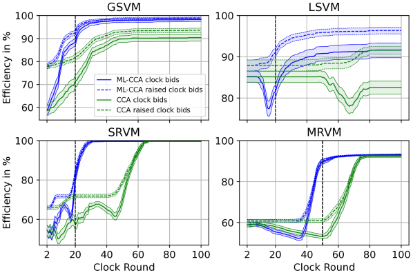
Figure 2: Efficiency path plots in SATS for ML-CCA and CCA both after clock bids (solid lines) and raised clock bids (dashed lines). Averaged over 100 runs including a 95% CI. The dashed black vertical line indicates the value of $Q^{\textrm{init}}$.

Results.

All efficiency results are presented in Table 1, while in Figure 2 we present the efficiency after each clock round, as well as the efficiency if those clock bids were enhanced with the clock bids raised heuristic (for $95$% CIs and $p$-values see Section D.7). In GSVM, ML-CCA’s clock phase exhibits over $7.8$% points higher efficiency compared to the CCA, while if we add the clock bids raised heuristic to both mechanisms, ML-CCA still exhibits over $5.3$% points higher efficiency. At the same time, ML-CCA is able to find clearing prices in $56$% of the instances, as opposed to only $3$% for the CCA. The results for LSVM are qualitatively very similar; ML-CCA’s clock phase increases efficiency compared to the CCA by over $9$% points, while clearing the market in $26$% of the cases as opposed to $0$%. If we add the clock bids raised heuristic to both mechanisms, ML-CCA still increases efficiency by over $4.7$% points. The SRVM domain, as suggested by the existence of only $3$ unique goods, is quite easy to solve. Thus, both mechanisms can achieve almost $100$% efficiency after their clock phase. For the clock bids raised heuristic our method reduces the efficiency loss by a factor of more than two (from $0.19$% to $0.07$%), and additionally, one can see from Figure 2 that our method reaches over $99$% in less than $30$ rounds. In MRVM, ML-CCA again achieves statistically significantly better results for all 3 bidding heuristics. Notably, the CCA needs both the clock bids raised heuristic and $38$ profit max bids to reach the same efficiency as our ML-CCA clock phase, i.e., it needs up to $138$ additional value queries per bidder (see Section D.7). In MRVM, LCPs never exist, thus neither ML-CCA nor the CCA can ever clear the market. To put our efficiency improvements in perspective, in the GSVM, LSVM and MRVM domains, ML-CCA’s clock phase achieves higher efficiency than the CCA enhanced with the clock bids raised heuristic, i.e., the CCA, even if it uses up to an additional $100$ value queries per bidder, cannot match the efficiency of our ML-powered clock phase. In Figure 2, we see that our ML-CCA can (almost) reach the efficiency numbers of Table 1 in a significantly reduced number of clock rounds compared to the CCA, while if we attempt to “speed up” the CCA, then its efficiency can substantially drop, see Section D.8. In particular, in GSVM and LSVM, using $50$ clock rounds, our ML-CCA can achieve higher efficiency than the CCA can in $100$ clock rounds.

7 Conclusion

We have proposed a novel method for training MVNNs to approximate the bidders’ value functions based on demand query observations. Additionally, we have framed the task of determining the price vector with the highest clearing potential as minimization of an objective function that we prove is convex, Lipschitz-continuous, a.e. differentiable, and whose gradient for linear prices has an intuitive economic interpretation: change the price of every good proportionally to its predicted under/over-demand at the current prices. The resulting mechanism (ML-CCA) from combining these two components exhibits significantly higher clearing potential than the CCA and can increase efficiency by up to $9$% points while at the same time converging in a much smaller number of rounds. Thus, we have designed the first practical ML-powered auction that employs the same interaction paradigm as the CCA, i.e., demand queries instead of cognitively too complex value queries, yet is able to significantly outperform the CCA in terms of both efficiency and clearing potential in realistic domains.

Appendix

Appendix A Payment and Activity Rules

In this section, we reprint the VCG and VCG-nearest payment rules, as well as give an overview of activity rules for the CCA, and argue why the most prominent choices are also applicable to our ML-CCA.

A.1 VCG Payments from Demand Query Data

Definition A.1.

(VCG Payments from Demand Query Data) Let $R=(R_{1},\ldots,R_{n})$ denote an elicited set of demand query data from each bidder and let $R_{-i}\coloneqq(R_{1},\ldots,R_{i-1},R_{i+1},\ldots,R_{n})$. We then calculate the VCG payments $\pi^{\text{VCG}}(R)=(\pi^{\text{VCG}}_{1}(R)\ldots,\pi^{\text{VCG}}_{n}(R))\in\mathbb{R}_{\geq 0}^{n}$ as follows:

$$\pi^{\text{VCG}}_{i}(R)\coloneqq$$ (12)

$$\sum_{j\in N\setminus\{i\}}\left\langle\left(p^{*}_{R_{-i}}\right)_{j},\left(a^{*}_{R_{-i}}\right)_{j}\right\rangle-\sum_{j\in N\setminus\{i\}}\left\langle\left(p^{*}_{R}\right)_{j},\left(a^{*}_{R}\right)_{j}\right\rangle.$$ (13)

where $a^{*}_{R_{-i}}$ is the allocation that maximizes the inferred social welfare (SW) when excluding bidder $i$, i.e.,

$$a^{*}_{R_{-i}}\in\operatorname*{argmax}_{\begin{subarray}{c}\mathcal{F}\,\ni\,\left(x_{j}^{*}\left(p^{(r_{j})}\right)\right)_{j\in N\setminus\{i\}}\\ :\,r_{j}\in\{1,\ldots,K\}\,\forall j\in N\setminus\{i\}\end{subarray}}\sum_{j\in N\setminus\{i\}}\left\langle p^{(r_{j})},x_{j}^{*}(p^{(r_{j})})\right\rangle,$$ (14)

and $p^{*}_{R_{-i}}=\left((p^{*}_{R_{-i}})_{1},\ldots,(p^{*}_{R_{-i}})_{n}\right)\in\mathbb{R}^{mn}_{\geq 0}$ denote the corresponding price vectors that lead to $a^{*}_{R_{-i}}$, and $a^{*}_{R}$ is a inferred-social-welfare-maximizing allocation (see Equation 2) with corresponding prices $p^{*}_{R}=\left((p^{*}_{R})_{1},\ldots,(p^{*}_{R})_{n}\right)\in\mathbb{R}^{mn}_{\geq 0}$.

Thus, when using VCG, bidder $i$’s utility is:

$$u_{i} =v_{i}((a_{R}^{*})_{i})-\pi^{\text{VCG}}_{i}(R)$$

$$=v_{i}((a_{R}^{*})_{i})+\sum_{j\in N\setminus\{i\}}\left\langle\left(p^{*}_{R}\right)_{j},\left(a^{*}_{R}\right)_{j}\right\rangle-\sum_{j\in N\setminus\{i\}}\left\langle\left(p^{*}_{R_{-i}}\right)_{j},\left(a^{*}_{R_{-i}}\right)_{j}\right\rangle.$$

Remark A.1.

Note that Definition A.1 defines VCG payments for a set of elicited demand query data $R$ using the bidders’ inferred values from this data set. Specifically, those would be the VCG payments after the CCA’s clock phase for example (i.e., if there was no supplementary round). However, one can analogously define VCG-payments for any given set of reported bundle-value pairs (see Weissteiner et al. (2023, Definition B.1.)). For example, in the case of additional value bids, such as supplementary round push bids, one would use Weissteiner et al. (2023, Definition B.1.) and set $\hat{v}_{i}(x^{r})=\max\{\left\langle x^{r},p^{r}\right\rangle,b_{i}^{s}(x^{r})\}$, where $b^{s}$ is the bidder’s supplementary round bid for that bundle (or zero, if she did not bid on it in the supplementary round), i.e., bidder $i$’s bid for any bundle is the maximum of her largest inferred value for that bundle based on the clock round bids and the supplementary round bids.

A.2 VCG-Nearest Payments

To define the VCG-nearest payments, we must first introduce the core:

Definition A.2.

(The Core) An outcome $(a,\pi)\in\mathcal{F}\times\mathbb{R}_{\geq 0}^{n}$ (i.e., a tuple of a feasible allocation $a$ and payments $\pi$) is in the core if it satisfies the following two properties:

1. The outcome is individual rational, i.e, $u_{i}=v_{i}(a_{i})-\pi_{i}\geq 0$ for all $i\in N$

2. The core constraints

   $$\forall\;L\subseteq N\;\sum_{i\in N\setminus L}\pi_{i}(R)\geq\max_{a^{\prime}\in\mathcal{F}}\sum_{i\in L}v_{i}(a^{\prime}_{i})-\sum_{i\in L}v_{i}(a_{i})$$ (15)

   where $v_{i}(a_{i})$ is bidder $i$’s value for bundle $a_{i}$ and $\mathcal{F}$ is the set of feasible allocations.

In words, a payment vector $\pi$ (together with a feasible allocation $a$) is in the core if no coalition of bidders $L\subset N$ is willing to pay more for the items than the mechanism is charging the winners. Note that by replacing the true values $v_{i}(a_{i})$ with the bidders’ (possibly untruthful) bids $b_{i}(a_{i})$ in Definition A.2 one can equivalently define the revealed core.

Now, we can define

Definition A.3.

(Minimum Revenue Core) Among all payment vectors in the (revealed) core, the (revealed) minimum revenue core is the set of payment vectors with smallest $L_{1}$-norm, i.e., which minimize the sum of the payments of all bidders.

We can now define VCG-nearest payments:

Definition A.4.

(VCG-Nearest Payments) Given an allocation $a_{R}$ for bidder reports $R$, the VCG-nearest payments $\pi^{\text{VCG-nearest}}(R)$ are defined as the vector of payments in the (revealed) minimum revenue core that minimizes the $L_{2}$-norm to the VCG payment vector $\pi^{\text{VCG}}(R)$.

A.3 On the Importance of Activity Rules to Align Incentives

In the CCA, activity rules serve multiple purposes. First, they can help speed up the auction process. Second, they reduce ”bid-sniping” opportunities, i.e., bidders concealing their true intentions until the very last rounds of the auction. Third, they can limit surprise bids in the supplementary round of the CCA and significantly reduce a bidder’s ability to drive up her opponents payments by overbidding on bundles that she can no longer win (Ausubel and Baranov 2017). There are two types of activity rules that are implemented in a CCA:

1. Clock phase activity rules, that limit the bundles that an agent can bid on during the clock phase, based on her bids in previous clock rounds.

2. Supplementary round activity rules, that restrict the amount that an agent can bid on for various sets of items during the supplementary round.

Most of the activity rules that were traditionally used for the clock phase of the CCA were based on either revealed-preference considerations or some points-based system, where the main idea is to assign points to each item prior to the auction, and only allow bidders to submit monotonically non-increasing in points bids, i.e., as the rounds progress and the prices increase, the bidders cannot submit bids for larger sets of items. Both of these approaches, as well as hybrid combinations thereof, were shown to actually further interfere with truthful bidding in some cases (Ausubel and Baranov 2014, 2020).

However, Ausubel and Baranov (2019) showed that basing the clock phase activity rule not on the above but instead entirely upon the generalized axiom of revealed preference (GARP) can dynamically approximate VCG payoffs and thus improve the bidding incentives of the CCA. GARP imposes revealed-preference constraints (see Definition A.5) to the bidder’s demand responses, i.e., the GARP activity rule requires the bidder to exhibit rational behaviour in her demand choices. Importantly, the GARP activity rule does not require a monotonic price trajectory. Thus, it can also be applied in our ML-powered clock phase, allowing the clock phase of our ML-CCA to enjoy the same improvement in bidding incentives.

For the supplementary round, the CCA’s most prominent activity rules are again based on a combination of the same points-based system and revealed-preference ideas. For this, we need to define the following constraint:

Definition A.5.

(Revealed-preference constraint) The revealed-preference constraint for bundle $x\in X$ with respect to clock round $r$ is

$$b_{i}(x)\leq b_{i}(x^{r})+\left\langle p^{r},x-x^{r}\right\rangle,$$ (16)

where $b_{i}(x)\in\mathbb{R}_{\geq 0}$ is bidder $i$’s bid for bundle $x\in X$ in the supplementary round, $x^{r}\in\mathcal{X}$ is the bundle demanded by the agent at clock round $r$, $b_{i}(x^{r})\in\mathbb{R}_{\geq 0}$ is the final bid for bundle $x^{r}\in\mathcal{X}$ and $p^{r}\in\mathbb{R}_{\geq 0}^{m}$ is the linear price vector of clock round $r$.

Intuitively, the revealed-preference constraint states that a bidder is not allowed to claim a high value for bundle $x\in\mathcal{X}$ relative to bundle $x^{r}\in\mathcal{X}$, given that she claimed to prefer bundle $x^{r}\in\mathcal{X}$ at clock round $r$ (see Inequality (6)). The difference between the three most prominent supplementary round activity rules is with respect to which clock rounds the revealed-preference constraint should be satisfied. Specifically:

1. Final Cap: A bid for bundle $x\in\mathcal{X}$ should satisfy the revealed-preference constraint (Definition A.5) with respect to the final clock round’s price $p^{Q^{\textrm{max}}}\in\mathbb{R}_{\geq 0}$ and bundle $x^{Q^{\textrm{max}}}\in\mathcal{X}$.

2. Relative Cap: A bid for bundle $x\in\mathcal{X}$ should satisfy the revealed-preference constraint (Definition A.5) with respect to the last clock round for which the bidder was eligible for that bundle $x\in\mathcal{X}$, based on the points-based system.

3. Intermediate Cap: A bid for bundle $x\in\mathcal{X}$ should satisfy the revealed-preference constraint (Definition A.5) with respect to all eligibility-reducing rounds, starting from the last clock round for which the bidder was eligible for $x\in\mathcal{X}$ based on the point system.

Ausubel and Baranov (2017) showed that combining the Final Cap and Relative Cap activity rules leads to the largest amount of reduction in bid-sniping opportunities for the UK 4G auction, as measured by the theoretical bid amount that each bidder would need to increase her bid by in the supplementary round in order to protect her final clock round bundle. Finally, note that the Final- and Intermediate Cap activity rules can also be applied to our ML-CCA.

To conclude, we observe that for both its clock phase and the supplementary round, our ML-CCA (with the same $F_{\text{init}}$ method as the CCA), is compatible with the most prominent activity rules for the corresponding phases of the CCA, while it is also obviously compatible with the most prominent payment rule, VCG-nearest prices (Definition A.4). This, combined with the fact that the ML-CCA has the same interaction paradigm for the bidders as the CCA, is a very strong indication that our ML-CCA can reduce the opportunities for the bidders to misreport to a similar extent as the classical CCA.

Appendix B Multiset MVNNs

B.1 Advantages of mMVNNs over MVNNs

In Weissteiner and Seuken (2020) and Weissteiner et al. (2022b, a, 2023) items with a capacity $c_{k}$, were treated as $c_{k}$ distinct items, without exploiting the prior knowledge that these $c_{k}$ items are indistinguishable to the bidders. Sufficiently large classical MVNNs that were trained on large enough training sets would at some point learn that these items are indistinguishable, but this prior information was not incorporated at an architectural level. For multiset MVNNs this hard prior knowledge is hard-coded directly into the architecture (see Definition 1). This additional prior knowledge is particularly beneficial for small training data sets in terms of generalization.

Also the MILPs solve times should be able to benefit from the reduced number of variables of mMVNNs compared to MVNNs. (For classical MVNNs one had to introduce one binary variable for each indistinguishable copy of an item, i.e., classical MVNNs got $\tilde{m}=\sum_{k=1}^{m}c_{k}$ binary variables at input, while mMVNNs get only $m$ integer variables as input.)

B.2 Universality of mMVNNs

Note that Weissteiner et al. (2022a) have proven universality of MVNNs only for the case of binary input vectors corresponding to classical sets (i.e., $c_{k}=1\ \forall k\in M$). Here, we prove in Section B.2 universality of mMVNNs for arbitrary capacities $c\in\mathbb{N}^{m}$ corresponding to multiset domains such as our $\mathcal{X}$.

First, we recall the following definition:

Definition B.1.

The set $\mathcal{V}$ of all monotonic and normalized functions from $\mathcal{X}$ to $\mathbb{R}_{\geq 0}$ is defined as

$$\mathcal{V}:=\{v_{i}:\mathcal{X}\to\mathbb{R}_{+}|\,\text{satisfy {\hyperref@@ii[itm:normalization]{(N)}{}} and {\hyperref@@ii[itm:monotonicity]{(M)}{}}}\}.$$ (17)

The following lemma says that every mMVNN is monotonic (M) and and normalized (N) in the sense of Definition B.1.

Lemma 1.

Let $\mathcal{M}_{i}^{\theta}:\mathcal{X}\to\mathbb{R}_{+}$ be an mMVNN from Definition 1. Then it holds that $\mathcal{M}_{i}^{(W^{i},b^{i})}\in\mathcal{V}$ for all $W^{i}\geq 0$ and $b^{i}\leq 0$.

Proof.

The proof of this lemma is perfectly analogous to the proof of (Weissteiner et al. 2022a, Lemma 1). ∎

Now we are ready to present a constructive proof for Theorem 1.

Proof of Theorem 1

Proof.

This proof follows a similar strategy as the proof of (Weissteiner et al. 2022a, Theorem 1).

1. $\mathcal{V}\supseteq\left\{\mathcal{M}_{i}^{(W^{i},b^{i})}:W^{i,k}\geq 0,b^{i,k}\leq 0\,\,\forall k\in\{1,\ldots,K_{i}\}\right\}$
   

   This direction follows immediately from Lemma 1.
   

2. $\mathcal{V}\subseteq\left\{\mathcal{M}_{i}^{(W^{i},b^{i})}:W^{i,k}\geq 0,b^{i,k}\leq 0\,\,\forall k\in\{1,\ldots,K_{i}\}\right\}$
   

   Let $(v_{i}(x))_{x\in\mathcal{X}}\in\mathcal{V}$. For the reverse direction, we give a constructive proof, i.e., we construct an mMVNN $\mathcal{M}_{i}^{\theta}$ with $\theta=(W^{i}_{v_{i}},b^{i}_{v_{i}})_{i\in\{1,\dots,4\}}$ such that $\mathcal{M}_{i}^{\theta}(x)=v_{i}(x)$ for all $x\in\mathcal{X}$.

   Let $(w_{j})_{j=1}^{|\mathcal{X}|}$ denote the values corresponding to $(v_{i}(x))_{x\in\mathcal{X}}$ of all $|\mathcal{X}|=\prod_{j=1}^{m}(c_{j}+1)$ possible bundles $x\in\mathcal{X}$ sorted by value in increasing order, i.e, let $x_{1}=(0,\ldots,0)$ with

   $$w_{1}:=v_{i}(x_{1})=0,$$ (18)

   let $x_{|\mathcal{X}|}=c=(c_{1},\ldots,c_{m})$ with

   $$w_{|\mathcal{X}|}:=v_{i}(x_{|\mathcal{X}|}),$$ (19)

   and $x_{j},x_{l}\in\mathcal{X}\setminus\{x_{1},x_{|\mathcal{X}|}\}$ for $1<l\leq j\leq|\mathcal{X}|-1$ with

   $$w_{j}:=v_{i}(x_{j})\,\leq\,w_{l}:=v_{i}(x_{l}).$$ (20)

   In the following, for $x_{l},x_{j}\in\mathcal{X}$, we use the notation $x_{l}\leq x_{j}$ iff $x_{l,k}\leq x_{j,k}\ \ \forall k\in M$. Thus, we write $x_{l}\not\leq x_{j}$ iff $\exists k\in M:x_{l,k}>x_{j,k}$, i.e., iff $x_{l}\leq x_{j}$ is not the case. Furthermore, we denote by $\left<\cdot,\cdot\right>$ the Euclidean scalar product on $\mathbb{R}^{m}$. Then, for all $x\in\mathcal{X}$:

   $$v_{i}(\xi)=\sum_{l=1}^{|\mathcal{X}|-1}\left(w_{l+1}-w_{l}\right)\text{1}_{\left\{\forall j\in\{1,\dots,l\}\,:\,\xi\not\leq x_{j}\right\}}$$ (21)

   $$=\sum_{l=1}^{|\mathcal{X}|-1}\left(w_{l+1}-w_{l}\right)\varphi_{0,1}{}\left(\sum_{j=1}^{l}\varphi_{0,1}{}\left(\sum_{k=1}^{m}\varphi_{0,1}(\xi_{k}-x_{j,k})\right)-(l-1)\right),$$ (22)

   where the second equality follows since

   $$\xi\not\leq x_{j} \iff\exists k\in M:\xi_{k}>x_{j,k}$$ (23)

   $$\iff\exists k\in M:\varphi_{0,1}(\xi_{k}-x_{j,k})=1$$ (24)

   $$\iff\varphi_{0,1}{}\left(\sum_{k=1}^{m}\varphi_{0,1}(\xi_{k}-x_{j,k})\right)=1,$$ (25)

   which implies that

   $$\left(\forall j\in\{1,\dots,l\}:\xi\not\leq x_{j}\right)$$

   $$\iff\sum_{j=1}^{l}\varphi_{0,1}{}\left(\sum_{k=1}^{m}\varphi_{0,1}(\xi_{k}-x_{j,k})\right)=l,$$ (26)

   and

   $$\text{1}_{\left\{\forall j\in\{1,\dots,l\}\,:\,x\not\leq x_{j}\right\}}$$

   $$=\varphi_{0,1}{}\left(\sum_{j=1}^{l}\varphi_{0,1}{}\left(\sum_{k=1}^{m}\varphi_{0,1}(\xi_{k}-x_{j,k})\right)-(l-1)\right).$$ (27)

   To match the structure of the mMVNN architecture defined in Definition 1, we can write $v_{i}(\xi)=v_{i}({\hyperref@@ii[itm:D]{\normalcolor D}}^{-1}\hyperref@@ii[itm:D]{\normalcolor D}\xi)$ and plug in ${\hyperref@@ii[itm:D]{\normalcolor D}}^{-1}\hyperref@@ii[itm:D]{\normalcolor D}\xi$ instead of $\xi$ in Equation 22.

   Equation 22 can be rewritten as the following mMVNN

   $$\mathcal{M}_{i}^{\theta}(x)=$$

   $$W^{i,4}_{v_{i}}\varphi_{0,1}{}\left(W^{i,3}_{v_{i}}\varphi_{0,1}{}\left(W^{i,2}_{v_{i}}\varphi_{0,1}{}\left(W^{i,1}_{v_{i}}\hyperref@@ii[itm:D]{\normalcolor D}\xi+b^{i,1}_{v_{i}}\right)+b^{i,2}_{v_{i}}\right)b^{i,3}_{v_{i}}\right)$$

   $$+b^{i,4}_{v_{i}}$$ (28)

   in the matrix-notation of Definition 1 with weight matrices and bias-vectors be given as:

   $$W_{v_{i}}^{i,1} :=\begin{bmatrix}\hyperref@@ii[itm:D]{\normalcolor D}^{-1}\\ \vdots\\ \hyperref@@ii[itm:D]{\normalcolor D}^{-1}\end{bmatrix}\in\mathbb{R}^{m(|\mathcal{X}|-1)\times m},$$ (29)

   $$b_{v_{i}}^{i,1} :=-\begin{bmatrix}x_{1}\\ x_{2}\\ \vdots\\ x_{|\mathcal{X}|-1}\end{bmatrix}\in\mathbb{R}^{m(|\mathcal{X}|-1)},$$ (30)

   $$\begin{split}W_{v_{i}}^{i,2}&:=\begin{bmatrix}\overbrace{1,\dots,1}^{m}&\overbrace{0,\dots,0}^{m}&\ldots&\overbrace{0,\dots,0}^{m}\\ 0,\dots,0&1,\dots,1&\ddots&\vdots\\ \vdots&\ddots&\ddots&0,\dots,0\\ 0,\dots,0&\ldots&0,\dots,0&1,\dots,1\end{bmatrix}\\ &\in\mathbb{R}^{(|\mathcal{X}|-1)\times m(|\mathcal{X}|-1)},\end{split}$$ (31)

   $$b_{v_{i}}^{i,2} :=0\in\mathbb{R}^{|\mathcal{X}|-1},$$ (32)

   $$W^{i,3}_{v_{i}} :=\begin{bmatrix}1&0&\ldots&0\\ \vdots&\ddots&\ddots&\vdots\\ \vdots&&\ddots&0\\ 1&\ldots&\ldots&1\end{bmatrix}\in\mathbb{R}^{(|\mathcal{X}|-1)\times(|\mathcal{X}|-1)},$$ (33)

   $$b_{v_{i}}^{i,3} :=\begin{bmatrix}0\\ -1\\ \vdots\\ -(|\mathcal{X}|-2)\end{bmatrix}\in\mathbb{R}^{|\mathcal{X}|-1},$$ (34)

   $$W_{v_{i}}^{i,4} :=\begin{bmatrix}w_{2}-w_{1}\\ w_{3}-w_{2}\\ \vdots\\ w_{|\mathcal{X}|}-w_{|\mathcal{X}|-1}\end{bmatrix}^{\top}\in\mathbb{R}^{1\times(|\mathcal{X}|-1)},$$ (35)

   $$b_{v_{i}}^{i,4} :=0\in\mathbb{R},$$ (36)

   where $W_{v_{i}}^{i,2}=\left(\text{1}_{\left\{(j-1)m<k\leq jm\right\}}\right)_{1\leq j\leq|\mathcal{X}|-1,1\leq k\leq m(|\mathcal{X}|-1)}$ is an alternative notation to describe Equation 31. Thus, $\mathcal{M}_{i}^{\theta}(x)$ is an mMVNN from Definition 1 with 6 layers in total (i.e., 1 input layer, 1 linear normalization layer D, 3 non-linear hidden layers and 1 output layer) and respective dimensions $[m,m,m(|\mathcal{X}|-1),|\mathcal{X}|-1,|\mathcal{X}|-1,1]$.

∎

Remark B.1 (Normalization Layer).

Note that our proof of Theorem 1 would also work without the linear normalization layer D. The normalization layer has the advantage that we can use similar hyperparameters as for classical MVNNs. E.g., we can use the same values of the parameters in the initialization scheme as provided in Weissteiner et al. (2023, Section 3.2 and Appendix E).

Remark B.2 (Number of Hidden Layers).

Note that for binary input vectors (corresponding to classical sets, i.e., $c=(1,\dots,1)$), 2 non-linear hidden layers were sufficient (Weissteiner et al. 2022a, Proof of Theorem 1), while for integer-valued input vectors (corresponding to multisets with capacities $c\in\mathbb{N}^{m}$), we used 3 non-linear hidden layers for our proof of Theorem 1. It is an interesting open question if 2 non-linear hidden layers would already be sufficient also for our multiset setting with capacities $c\in\mathbb{N}^{m}$.

Remark B.3 (Number of Hidden Neurons).

The dimension $[m,m,m(|\mathcal{X}|-1),|\mathcal{X}|-1,|\mathcal{X}|-1,1]$ of the mMVNN used in the proof of Theorem 1 is just an upper bound. This proof does not imply that such large networks are actually. From a theoretical perspective it is interesting that this upper bound is finite, while for NNs on continuous domains no finite upper bound for perfect approximation exits. In practice much smaller networks are usually sufficient. All the results reported in this paper were achieved by much smaller networks with at most 30 neurons per layer (see Table 2 in Section D.3).

Appendix C ML-powered Demand Query Generation:Theoretical Results

In this section, we prove Theorems 2 and 3.

C.1 Proof of Theorem 2

In this subsection, we first present and prove in Lemma 2 an unconstrained version of Theorem 2, which we later use to prove our main statement from Theorem 2.

Lemma 2 extends (Bikhchandani and Ostroy 2002, Theorem 3.1.). Concretely, we additionally show that if linear clearing prices exist, every minimizer of $W$ is a clearing price (while Bikhchandani and Ostroy (2002, Theorem 3.1.) only showed that every clearing price $p$ minimizes $W$ not specifying if there could be other minimizers of $W$ which are not clearing prices).

Lemma 2.

Consider the notation from Definitions 2 and 3 and the objective function $W(p,v)\coloneqq R(p)+\sum_{i\in N}U(p,v_{i})$. Then it holds that, if a linear clearing price exists, every price vector

$$p^{\prime}\in\operatorname*{argmin}_{\tilde{p}\in\mathbb{R}_{\geq 0}^{m}}W(\tilde{p},v)$$ (37)

is a clearing price and the corresponding allocation $a(p^{\prime})\in\mathcal{F}$ is efficient.

Proof of Lemma 2.

We first show in Item 1 that for clearing prices $p\in\mathbb{R}_{\geq 0}^{m}$, the corresponding allocation $a(p)\in\mathcal{F}$ is efficient. Next, in Item 2 we show that every linear clearing price $p\in\mathbb{R}_{\geq 0}^{m}$ minimizes $W$, i.e., formally $p\in\operatorname*{argmin}_{\tilde{p}\in\mathbb{R}_{\geq 0}^{m}}W(\tilde{p},v)$. Finally, in Item 3 we show that if linear clearing prices exist, any minimizer of $W$ is in fact a linear clearing price.

1. Let $(p,a(p))\in\mathbb{R}^{m}_{\geq 0}\times\mathcal{F}$ be clearing prices and the corresponding supported allocation (see Definition 3). Furthermore, let $\tilde{a}\in\mathcal{F}$ be any other feasible allocation. Then it holds that:

   $$\sum_{i=1}^{n}v_{i}(a_{i}(p))=$$ (38)

   $$\sum_{i=1}^{n}[v_{i}(a_{i}(p))-\left\langle p,a_{i}(p)\right\rangle]+\sum_{i=1}^{n}\left\langle p,a_{i}(p)\right\rangle=$$ (39)

   $$\left(\sum_{i=1}^{n}U(p,v_{i})\right)+R(p)\geq$$ (40)

   $$\sum_{i=1}^{n}[v_{i}(\tilde{a}_{i})-\left\langle p,\tilde{a}_{i}\right\rangle]+\sum_{i=1}^{n}\left\langle p,\tilde{a}_{i}\right\rangle=$$ (41)

   $$\sum_{i=1}^{n}v_{i}(\tilde{a}_{i}),$$ (42)

   where the first inequality follows since $(p,a(p))$ are clearing prices and fulfill Items 1 and 2 in Definition 3 and because $\tilde{a}\in\mathcal{F}$ is another feasible allocation. This shows that a supported allocation $a(p)$ is efficient.

2. Let $(p,a(p))\in\mathbb{R}^{m}_{\geq 0}\times\mathcal{F}$ be clearing prices and the corresponding supported allocation (see Definition 3). Furthermore, let $\tilde{p}\in\mathbb{R}_{\geq 0}^{m}$ be any other linear prices. Then it holds that:

   $$W(p,v)=$$ (43)

   $$\max_{a\in\mathcal{F}}\left\{\sum_{i=1}^{n}\left\langle p,a_{i}\right\rangle\right\}+\sum_{i=1}^{n}\max_{x\in\mathcal{X}}\left\{v_{i}(x)-\left\langle p,x\right\rangle\right\}=$$ (44)

   $$\sum_{i=1}^{n}\left\langle p,a_{i}(p)\right\rangle+\sum_{i=1}^{n}[v_{i}(a_{i}(p))-\left\langle p,a_{i}(p)\right\rangle]=$$ (45)

   $$\sum_{i=1}^{n}v_{i}(a_{i}(p))=$$ (46)

   $$\sum_{i=1}^{n}\left\langle\tilde{p},a_{i}(p)\right\rangle+\sum_{i=1}^{n}[v_{i}(a_{i}(p))-\left\langle\tilde{p},a_{i}(p)\right\rangle]\leq$$ (47)

   $$\max_{a\in\mathcal{F}}\left\{\sum_{i=1}^{n}\left\langle\tilde{p},a_{i}\right\rangle\right\}+\sum_{i=1}^{n}\max_{x\in\mathcal{X}}\left\{v_{i}(x)-\left\langle\tilde{p},x\right\rangle\right\}=$$ (48)

   $$W(\tilde{p},v),$$ (49)

   where Equation 44 follows by definition of $W$ and Equation 45 follows since $(p,a(p))$ are clearing prices and the corresponding supported allocation, respectively Thus, we get that

   $$W(p,v)\leq W(\tilde{p},v),$$ (50)

   for all linear prices $\tilde{p}\in\mathbb{R}_{\geq 0}^{m}$, which concludes the proof.

3. Let $p^{\prime}\in\operatorname*{argmin}_{\tilde{p}\in\mathbb{R}_{\geq 0}^{m}}W(\tilde{p},v)$ be a minimizer of $W$. Moreover, let $p\in\mathbb{R}_{\geq 0}^{m}$ denote a linear clearing price and let $a(p)\in\mathcal{F}$ be the corresponding supported allocation (see Definition 3). Furthermore, let $x_{i}^{*}(p^{\prime})\in\operatorname*{argmax}_{x\in\mathcal{X}}\left\{v_{i}(x)-\left\langle p^{\prime},x\right\rangle\right\}\,\forall i\in N$. We know from Item 2 that $W(p^{\prime},v)=W(p,v)$. Furthermore, we get that

   $$\sum_{i=1}^{n}v_{i}(x_{i}^{*}(p^{\prime}))-\sum_{i=1}^{n}\left\langle p^{\prime},x_{i}^{*}(p^{\prime})\right\rangle+\left\langle p^{\prime},c\right\rangle=$$ (51a)

   $$W(p^{\prime},v)=W(p,v)=$$ (51b)

   $$\sum_{i=1}^{n}v_{i}(a_{i}(p))-\sum_{i=1}^{n}\left\langle p,a_{i}(p)\right\rangle+\left\langle p,c\right\rangle\stackrel{{\scriptstyle\eqref{eq:app:proof:thm1:itm3:3}}}{{=}}$$ (51c)

   $$\sum_{i=1}^{n}v_{i}(a_{i}(p))=$$ (51d)

   $$\sum_{i=1}^{n}v_{i}(a_{i}(p))-\sum_{i=1}^{n}\left\langle p^{\prime},a_{i}(p)\right\rangle+\left\langle p^{\prime},c\right\rangle,$$ (51e)

   where the last equation follows since $a(p)$ is a clearing allocation supported by $p$ and thus $\sum_{i=1}^{n}\left\langle p^{\prime},a_{i}(p)\right\rangle=\left\langle p^{\prime},c\right\rangle$. Next, we can subtract $\left\langle p^{\prime},c\right\rangle$ from both sides of Equation 51 to obtain

   $$\sum_{i=1}^{n}v_{i}(x_{i}^{*}(p^{\prime}))-\left\langle p^{\prime},x_{i}^{*}(p^{\prime})\right\rangle=$$

   $$\sum_{i=1}^{n}v_{i}(a_{i}(p))-\left\langle p^{\prime},a_{i}(p)\right\rangle.$$ (52)

   Moreover, from the optimality of $x_{i}^{*}(p^{\prime})$ it follows that

   $$v_{i}(x_{i}^{*}(p^{\prime}))-\left\langle p^{\prime},x_{i}^{*}(p^{\prime})\right\rangle\geq v_{i}(a_{i}{(p)})-\left\langle p^{\prime},a_{i}{}(p)\right\rangle,$$ (53)

   holds for every $i\in\{1,\dots,n\}$.

   Using now Equations 52 and 53, it follows that for every $i\in\{1,\dots,n\}$

   $$U(p^{\prime},v_{i})=v_{i}(x_{i}^{*}(p^{\prime}))-\left\langle p^{\prime},x_{i}^{*}(p^{\prime})\right\rangle=$$ (54)

   $$v_{i}(a_{i}(p))-\left\langle p^{\prime},a_{i}(p)\right\rangle.$$ (55)

   Taken all together, since $\sum_{i\in N}\left\langle p^{\prime},a_{i}(p)\right\rangle=\sum_{j\in M}\left\langle p^{\prime}_{j},c_{j}\right\rangle=R(p^{\prime})$ and $U(p^{\prime},v_{i})=v_{i}(a_{i}(p))-\left\langle p^{\prime},a_{i}(p)\right\rangle$ for all $i\in N$ , we can conclude that $(p^{\prime},a(p))\in\mathbb{R}^{m}_{\geq 0}\times\mathcal{F}$ by Definition 3 is a linear clearing price with corresponding supported allocation $a(p)\in\mathcal{F}$. This finalizes the proof of Lemma 2.

∎

Now, we are ready to prove Theorem 2, which follows almost immediately from Lemma 2.

Proof of Theorem 2.

Let $p^{\prime}$ be a solution to the constrained minimization problem defined by Equation 9. Moreover, let $p\in\mathbb{R}_{\geq 0}^{m}$ denote a linear clearing price vector and let $a(p)\in\mathcal{F}$ be the corresponding supported allocation (see Definition 3).

In Item 2 in the proof of Lemma 2, we have seen that $p$ minimizes $W$ without any constraints. The clearing price vector $p$ obviously satisfies constraint (9b), thus $p$ is also a solution to the constrained optimization problem (9). Therefore, in the case that linear clearing prices exist the minimal objective value of the constrained optimization problem from (9) is equal to the minimal objective value of the unconstrained minimization problem (37). From this we can conclude that in the case that linear clearing prices exist, every solution $p^{\prime}$ of (9) is also a solution of the optimization problem (37). Finally, Lemma 2 tells us that every solution $p^{\prime}$ of the optimization problem (37) is a clearing price and $a(p^{\prime})$ is efficient. ∎

In Theorem 2 we proved that the constraint minimizer of $W$ has the same economical favourable properties as the unconstrained minimizer of $W$ if linear clearing prices exist. Thus, we do not lose anything in cases where linear clearing prices exist, while due to the constraint (9b) we have the advantage of receiving feasible allocations in the case that no linear clearing price exist.

C.2 Details: Proof of Theorem 3

Before we start with the proof, we will quickly provide a proof for Equation 8, since this equation (that we have not explicitly proven in the main paper) is essential in the proof of Theorem 3.

Proof of Equation 8.

$$R(p) \coloneqq\max\limits_{a\in\mathcal{F}}\left\{\sum\limits_{i\in N}\left\langle p,a_{i}\right\rangle\right\}$$ (56)

$$=\max\limits_{a\in\mathcal{F}}\left\{\sum\limits_{i\in N}\sum_{j\in M}p_{j}a_{i,j}\right\}$$ (57)

$$=\max\limits_{a\in\mathcal{F}}\left\{\sum_{j\in M}\sum_{i\in N}p_{j}a_{i,j}\right\}$$ (58)

$$=\max\limits_{a\in\mathcal{F}}\left\{\sum_{j\in M}p_{j}\sum_{i\in N}a_{i,j}\right\}$$ (59)

$$=\max\left\{\sum_{j\in M}p_{j}\sum_{i\in N}a_{i,j}:\sum_{i\in N}a_{i,j}\leq c_{j}\ \forall j\in M\right\}$$ (60)

$$=\sum\limits_{j\in M}p_{j}c_{j}=\sum\limits_{j\in M}c_{j}p_{j}=\left\langle c,p\right\rangle.$$ (61)

∎

In the first lemma we prove that $p\mapsto W(p,\left(\mathcal{M}_{i}^{\theta}\right)_{i=1}^{n})$ is Lipschitz-continuous. While neither $p\mapsto x^{*}_{i}(p)$, nor $p\mapsto\mathcal{M}_{i}^{\theta}(x^{*}_{i}(p))$ nor $p\mapsto\left\langle p,x^{*}_{i}(p)\right\rangle$ are continuous, (surprisingly) $p\mapsto\mathcal{M}_{i}^{\theta}(x^{*}_{i}(p))+\left\langle p,x^{*}_{i}(p)\right\rangle$ is continuous.

Lemma 3 (Continuity).

The map $p\mapsto W\left(p,\left(\mathcal{M}_{i}^{\theta}\right)_{i=1}^{n}\right)$ from $\mathbb{R}_{\geq 0}^{m}$ to $\mathbb{R}_{\geq 0}$ is Lipschitz-continuous with Lipschitz-constant $(n+1)\left\|{c}\right\|_{2}$.

Proof.

Since $W\left(p,\left(\mathcal{M}_{i}^{\theta}\right)_{i=1}^{n}\right)\coloneqq R(p)+\sum_{i\in N}U\left(p,\mathcal{M}_{i}^{\theta}\right)$ is the sum of $1+n$ functions, we first quickly show that $R$ is Lipschitz-continuous in $p$ and afterwards we will show that also $U$ is Lipschitz-continuous in $p$.

From Equation 8 it follows that $R(p)=\sum\limits_{j\in M}c_{j}p_{j}$ is linear in $p$ and thus Lipschitz-continuous with Lipschitz-constant $\left\|{c}\right\|_{2}$.

In the remainder of the proof we are going to show that $U\left(p,\mathcal{M}_{i}^{\theta}\right)\coloneqq\max\limits_{x\in\mathcal{X}}\left\{\mathcal{M}_{i}^{\theta}(x)-\left\langle p,x\right\rangle\right\}$ is Lipschitz-continuous in $p$. Let $p,\tilde{p}\in\mathbb{R}_{\geq 0}^{m}$ be two price vectors, then we have

$$U\left(\tilde{p},\mathcal{M}_{i}^{\theta}\right) \geq\mathcal{M}_{i}^{\theta}(\hat{x}^{*}_{i}(p))+\left\langle\tilde{p},\hat{x}^{*}_{i}(p)\right\rangle$$ (62)

$$=\mathcal{M}_{i}^{\theta}(\hat{x}^{*}_{i}(p))+\left\langle\tilde{p}+p-p,\hat{x}^{*}_{i}(p)\right\rangle$$ (63)

$$=\mathcal{M}_{i}^{\theta}(\hat{x}^{*}_{i}(p))+\left\langle p,\hat{x}^{*}(p)\right\rangle+\left\langle\tilde{p}-p,\hat{x}^{*}_{i}(p)\right\rangle$$ (64)

$$=U\left(p,\mathcal{M}_{i}^{\theta}\right)+\left\langle\tilde{p}-p,\hat{x}^{*}_{i}(p)\right\rangle$$ (65)

$$\geq U\left(p,\mathcal{M}_{i}^{\theta}\right)-\left\|{\tilde{p}-p}\right\|_{2}\left\|{\hat{x}^{*}_{i}(p)}\right\|_{2}$$ (66)

$$\geq U\left(p,\mathcal{M}_{i}^{\theta}\right)-\left\|{\tilde{p}-p}\right\|_{2}\left\|{c}\right\|_{2},$$ (67)

and thus

$$U\left(\tilde{p},\mathcal{M}_{i}^{\theta}\right)-U\left(p,\mathcal{M}_{i}^{\theta}\right)\geq-\left\|{\tilde{p}-p}\right\|_{2}\left\|{c}\right\|_{2}.$$ (68)

By exchanging the roles of $p$ and $\tilde{p}$, we also obtain $U\left(p,\mathcal{M}_{i}^{\theta}\right)\geq U\left(\tilde{p},\mathcal{M}_{i}^{\theta}\right)-\left\|{\tilde{p}-p}\right\|_{2}\left\|{c}\right\|_{2}$ and thus,

$$U\left(\tilde{p},\mathcal{M}_{i}^{\theta}\right)-U\left(p,\mathcal{M}_{i}^{\theta}\right)\leq\left\|{\tilde{p}-p}\right\|_{2}\left\|{c}\right\|_{2}.$$ (69)

Finally, Equations 68 and 69 together imply

$$\left|U\left(\tilde{p},\mathcal{M}_{i}^{\theta}\right)-U\left(p,\mathcal{M}_{i}^{\theta}\right)\right|\leq\left\|{\tilde{p}-p}\right\|_{2}\left\|{c}\right\|_{2}.$$ (70)

Equation 70 by definition says that $U$ is Lipschitz-continuous in $p$ with Lipschitz-constant $\left\|{c}\right\|_{2}$.

So, we finally obtain, that $W$ is Lipschitz-continuous in $p$ with Lipschitz-constant $(n+1)\left\|{c}\right\|_{2}$. ∎

Lemma 4 (Convexity).

The map $p\mapsto W\left(p,\left(\mathcal{M}_{i}^{\theta}\right)_{i=1}^{n}\right)$ from $\mathbb{R}_{\geq 0}^{m}$ to $\mathbb{R}_{\geq 0}$ is convex.

Proof.

Since $W\left(p,\left(\mathcal{M}_{i}^{\theta}\right)_{i=1}^{n}\right)\coloneqq R(p)+\sum_{i\in N}U\left(p,\mathcal{M}_{i}^{\theta}\right)$ is the sum of $1+n$ functions, we first quickly show that $R$ is obviously convex in $p$ and afterwards we will show that also $U$ is convex in $p$.

From Equation 8 it follows that $R(p)=\sum\limits_{j\in M}c_{j}p_{j}$ is linear in $p$ and thus convex in $p$.

In the remainder of the proof we are going to show that $U\left(p,\mathcal{M}_{i}^{\theta}\right)\coloneqq\max\limits_{x\in\mathcal{X}}\left\{\mathcal{M}_{i}^{\theta}(x)-\left\langle p,x\right\rangle\right\}$ is convex in $p$. For every $i\in N$ and for every $x\in\mathcal{X}$, the map $p\mapsto\mathcal{M}_{i}^{\theta}(x)-\left\langle p,x\right\rangle$ is (affine-)linear in $p$ and thus convex in $p$. As the maximum over convex functions is always convex (Danskin 1967; Bertsekas 1971, 1999), $U\left(p,\mathcal{M}_{i}^{\theta}\right)\coloneqq\max\limits_{x\in\mathcal{X}}\left\{\mathcal{M}_{i}^{\theta}(x)-\left\langle p,x\right\rangle\right\}$ is convex in $p$.

So finally we get that $W$ is convex in $p$, since it is the sum of $(n+1)$ convex functions. ∎

Lemma 5 (Sub-gradients).

Let $\hat{\mathcal{X}}^{*}_{i}(p):=\operatorname*{argmax}_{x\in\mathcal{X}}\left\{\mathcal{M}_{i}^{\theta}(x)-\left\langle p,x\right\rangle\right\}$ denote the set of utility maximizing bundles w.r.t. $\mathcal{M}_{i}^{\theta}$ for the $i$-th bidder. Then the sub-gradients of the map $p\mapsto W\left(p,\left(\mathcal{M}_{i}^{\theta}\right)_{i=1}^{n}\right)$ from $\mathbb{R}_{\geq 0}^{m}$ to $\mathbb{R}_{\geq 0}$ are given by

$$\nabla^{\textnormal{sub}}_{p}W(p,\left(\mathcal{M}_{i}^{\theta}\right)_{i=1}^{n})\\ :=\operatorname{conv}\left\{c-\sum_{i\in N}\hat{x}^{*}_{i}(p):\left(\hat{x}^{*}_{i}(p)\right)_{i\in N}\in\bigtimes_{i\in N}\hat{\mathcal{X}}^{*}_{i}(p)\right\},$$ (71)

where $\operatorname{conv}$ denotes the convex hull and $\bigtimes$ denotes the Cartesian product. In particular, for each $\left(\hat{x}^{*}_{i}(p)\right)_{i\in N}\in\bigtimes_{i\in N}\hat{\mathcal{X}}^{*}_{i}(p)$,

$$c-\sum_{i\in N}\hat{x}^{*}_{i}(p)\in\nabla^{\textnormal{sub}}_{p}W(p,\left(\mathcal{M}_{i}^{\theta}\right)_{i=1}^{n})$$ (72)

is a subgradient of $W$ with respect to $p$.

Proof.

Since $W\left(p,\left(\mathcal{M}_{i}^{\theta}\right)_{i=1}^{n}\right)\coloneqq R(p)+\sum_{i\in N}U\left(p,\mathcal{M}_{i}^{\theta}\right)$ is the sum of $1+n$ functions, we first quickly compute the (sub-)gradient of $R$ with respect to $p$ and afterwards we will compute the sub-gradients of $U$ with respect to $p$.

From Equation 8 it follows that $R(p)=\sum\limits_{j\in M}c_{j}p_{j}$ is linear in $p$ and thus its sub-gradient is uniquely defined as its gradient $\nabla_{p}R(p)=c$, i.e., $\nabla^{\textnormal{sub}}_{p}R(p)=\{c\}$.

In the remainder of the proof we are going to compute the set of sub-gradients of $U\left(p,\mathcal{M}_{i}^{\theta}\right)\coloneqq\max\limits_{x\in\mathcal{X}}\left\{\mathcal{M}_{i}^{\theta}(x)-\left\langle p,x\right\rangle\right\}$ with respect to $p$ with the help of Danskin’s theorem (originally proven by Danskin (1967) and later refined by Bertsekas (1971, 1999)). Let’s define $\phi_{i}(p,x):=\mathcal{M}_{i}^{\theta}(x)-\left\langle p,x\right\rangle$. Then $U\left(p,\mathcal{M}_{i}^{\theta}\right)=\max\limits_{x\in\mathcal{X}}\phi_{i}(p,x)$ and $\hat{\mathcal{X}}^{*}_{i}(p)=\operatorname*{argmax}\limits_{x\in\mathcal{X}}\phi_{i}(p,x)$. Next, we show that $\phi_{i}:\mathbb{R}_{\geq 0}^{m}\times\mathcal{X}\to\mathbb{R}$ fulfills all the assumptions of Danskin’s theorem:

• For every $x\in\mathcal{X}$ the map $p\mapsto\phi_{i}(p,x)$ is convex and differentiable, since it is (affine-)linear.

• For every $p\in\mathbb{R}_{\geq 0}^{m}$ the map $x\mapsto\phi_{i}(p,x)$ is continuous, since $\mathcal{X}$ is discrete and every function is continuous with respect to the discrete topology.

• Furthermore, the set $\mathcal{X}$ is compact (since it is finite).

Under these three assumptions Danskin’s theorem tells us that

$$\nabla^{\textnormal{sub}}_{p}U\left(p,\mathcal{M}_{i}^{\theta}\right)=\operatorname{conv}\left\{\nabla_{p}\phi_{i}(p,x):x\in\hat{\mathcal{X}}^{*}_{i}(p)\right\}.$$ (73)

Now we can simply compute $\nabla_{p}\phi_{i}(p,x)$ for any constant $x\in\mathcal{X}$, i.e.,

$$\nabla_{p}\phi_{i}(p,x) =\nabla_{p}\left(\mathcal{M}_{i}^{\theta}(x)-\left\langle p,x\right\rangle\right)$$ (74a)

$$=\nabla_{p}\mathcal{M}_{i}^{\theta}(x)-\nabla_{p}\left\langle p,x\right\rangle$$ (74b)

$$=0-x=-x.$$ (74c)

Plugging in Equation 74 into Equation 73 results in

$$\nabla^{\textnormal{sub}}_{p}U\left(p,\mathcal{M}_{i}^{\theta}\right)=\operatorname{conv}\left\{-x:x\in\hat{\mathcal{X}}^{*}_{i}(p)\right\}.$$ (75)

Note that set of sub-gradients of a sum of real-valued convex functions, is equal to the sum of the sets of sub-gradients of the individual functions (Rockafellar 1970, Theorem 23.8). Further note that the sum of convex hulls of sets is equal to the convex hull of their sum. We use these two insights and Equation 75 to finally compute the set of sub-gradients

$$\nabla^{\textnormal{sub}}_{p}W(p,\left(\mathcal{M}_{i}^{\theta}\right)_{i=1}^{n})=$$ (76a)

$$=\nabla^{\textnormal{sub}}\left(R(p)+\sum_{i\in N}U\left(p,\mathcal{M}_{i}^{\theta}\right)\right)$$ (76b)

$$=\nabla^{\textnormal{sub}}R(p)+\sum_{i\in N}\nabla^{\textnormal{sub}}U\left(p,\mathcal{M}_{i}^{\theta}\right)$$ (76c)

$$=\{c\}+\sum_{i\in N}\operatorname{conv}\left\{-x:x\in\hat{\mathcal{X}}^{*}_{i}(p)\right\}$$ (76d)

$$=\{c\}+\operatorname{conv}{\sum_{i\in N}\left\{-x:x\in\hat{\mathcal{X}}^{*}_{i}(p)\right\}}$$ (76e)

$$=\{c\}-\operatorname{conv}{\sum_{i\in N}\hat{\mathcal{X}}^{*}_{i}(p)}$$ (76f)

$$=\{c\}-\operatorname{conv}{\left\{\sum_{i\in N}\hat{x}^{*}_{i}(p):\left(\hat{x}^{*}_{i}(p)\right)_{i\in N}\in\bigtimes_{i\in N}\hat{\mathcal{X}}^{*}_{i}(p)\right\}}$$ (76g)

$$=\operatorname{conv}{\left\{c-\sum_{i\in N}\hat{x}^{*}_{i}(p):\left(\hat{x}^{*}_{i}(p)\right)_{i\in N}\in\bigtimes_{i\in N}\hat{\mathcal{X}}^{*}_{i}(p)\right\}},$$ (76h)

which proves the main statement (71) of Lemma 5. This directly implies that for each $\left(\hat{x}^{*}_{i}(p)\right)_{i\in N}\in\bigtimes_{i\in N}\hat{\mathcal{X}}^{*}_{i}(p)$,

$$c-\sum_{i\in N}\hat{x}^{*}_{i}(p)\in\nabla^{\textnormal{sub}}_{p}W(p,\left(\mathcal{M}_{i}^{\theta}\right)_{i=1}^{n})$$ (77)

is an element of the convex hull in (76h) and thus a sub-gradient of $W$ with respect to $p$. ∎

Next, Lemma 6 shows that the map $p\mapsto W\left(p,\left(\mathcal{M}_{i}^{\theta}\right)_{i=1}^{n}\right)$ from $\mathbb{R}_{\geq 0}^{m}$ to $\mathbb{R}_{\geq 0}$ is Lebesgue-almost everywhere differentiable with (proper) gradient

$$\nabla_{p}W(p,\left(\mathcal{M}_{i}^{\theta}\right)_{i=1}^{n})\stackrel{{\scriptstyle\mathrm{a.e.}}}{{=}}c-\sum_{i\in N}\hat{x}^{*}_{i}(p),$$ (78)

where $\hat{x}^{*}_{i}(p)\in\hat{\mathcal{X}}^{*}_{i}(p):=\operatorname*{argmax}_{x\in\mathcal{X}}\left\{\mathcal{M}_{i}^{\theta}(x)-\left\langle p,x\right\rangle\right\}$ denotes the utility maximizing bundle w.r.t. $\mathcal{M}_{i}^{\theta}$ for the $i$-th bidder, which is Lebesgue-almost everywhere unique.

Lemma 6 (A.e. Differentiable).

Let $\left(\mathcal{M}_{i}^{\theta}\right)_{i=1}^{n}$ be a tuple of mMVNNs. Then there exists a dense subset $P\subseteq\mathbb{R}_{\geq 0}^{m}$ such that $\mathbb{R}_{\geq 0}^{m}\setminus P$ is a Lebesgue null set, and that $\forall p\in P:$

1. A unique optimizer $\hat{x}^{*}_{i}(p)\in\hat{\mathcal{X}}^{*}_{i}(p)$ exists, i.e.,

   $$\left\{x^{*}_{i}(p)\right\}=\hat{\mathcal{X}}^{*}_{i}(p):=\operatorname*{argmax}_{x\in\mathcal{X}}\left\{\mathcal{M}_{i}^{\theta}(x)-\left\langle p,x\right\rangle\right\}$$ (79)

   and

2. the map $p\mapsto W\left(p,\left(\mathcal{M}_{i}^{\theta}\right)_{i=1}^{n}\right)$ is differentiable with gradient

   $$\nabla_{p}W(p,\left(\mathcal{M}_{i}^{\theta}\right)_{i=1}^{n})=c-\sum_{i\in N}\hat{x}^{*}_{i}(p),$$ (80)

   which is also the unique sub-gradient, i.e. $\left\{c-\sum_{i\in N}\hat{x}^{*}_{i}(p)\right\}=\nabla^{\textnormal{sub}}_{p}W(p,\left(\mathcal{M}_{i}^{\theta}\right)_{i=1}^{n})$.

3. The unique optimizer $\hat{x}^{*}_{i}(p)$ is constant in a local neighborhood of $p$, and thus $\partial_{p}\hat{x}^{*}_{i}(p)=0$.

Proof.

We start this proof by defining $P$ and showing a.e. differentiability. Since $W\left(p,\left(\mathcal{M}_{i}^{\theta}\right)_{i=1}^{n}\right)\coloneqq R(p)+\sum_{i\in N}U\left(p,\mathcal{M}_{i}^{\theta}\right)$ is the sum of $1+n$ functions, we first quickly show that $R$ is obviously differentiable and afterwards we show that each $U\left(p,\mathcal{M}_{i}^{\theta}\right)$ is differentiable on a set $P_{i}$. Afterwards we will define $P$ as their intersection.

From Equation 8 it follows that $R(p)=\sum\limits_{j\in M}c_{j}p_{j}$ is linear in $p$ and thus differentiable.

Next, we show that $U\left(p,\mathcal{M}_{i}^{\theta}\right)\coloneqq\max\limits_{x\in\mathcal{X}}\left\{\mathcal{M}_{i}^{\theta}(x)-\left\langle p,x\right\rangle\right\}$ is differentiable a.e. and define $P_{i}$. We know already from the proof of Lemma 4 that $U\left(p,\mathcal{M}_{i}^{\theta}\right)$ is convex and Rockafellar (1970, Theorem 25.5 on p. 246) tells us that for any real-valued convex function there exists a dense set $P_{i}$ on which the functions is differentiable with the complement of $P_{i}$ being a null set. Thus, for each $p\mapsto U\left(p,\mathcal{M}_{i}^{\theta}\right),\,i\in N$, we obtain such a $P_{i}$. If $1+n\in\mathbb{N}$ functions are differentiable at a point $p$, then their sum is too. Thus, $p\mapsto W\left(p,\left(\mathcal{M}_{i}^{\theta}\right)_{i=1}^{n}\right)$ is differentiable on $P:=\bigcap_{i=1}^{n}P_{i}$. Since each $P_{i}$ is dense in $\mathbb{R}_{\geq 0}^{m}$, $P$ is also dense in $\mathbb{R}_{\geq 0}^{m}$. Moreover, it holds that $\lambda^{m}\left(\mathbb{R}_{\geq 0}^{m}\setminus P\right)=\lambda^{m}\left(\bigcup_{i=1}^{n}(\mathbb{R}_{\geq 0}^{m}\setminus P_{i})\right)\leq\sum_{i=1}^{n}\lambda^{m}\left(\mathbb{R}_{\geq 0}^{m}\setminus P_{i}\right)=\sum_{i=1}^{n}0=0$, i.e., the $m$-dimensional Lebesgue measure of $\mathbb{R}_{\geq 0}^{m}\setminus P$ vanishes. Putting everything together, we get that $p\mapsto W\left(p,\left(\mathcal{M}_{i}^{\theta}\right)_{i=1}^{n}\right)$ is a.e. differentiable (concretely differentiable for all $p\in P$).

Next, we prove the uniqueness of $\hat{x}^{*}_{i}(p)\in\hat{\mathcal{X}}^{*}_{i}(p)$ for every $p\in P_{i}\supseteq P$. We know that $p\mapsto U\left(p,\mathcal{M}_{i}^{\theta}\right)$ is differentiable at $p\in P_{i}$, and thus we know that the sub-gradient is unique, i.e., $\left|\nabla^{\textnormal{sub}}_{p}U\left(p,\mathcal{M}_{i}^{\theta}\right)\right|=\left|\left\{\nabla_{p}U\left(p,\mathcal{M}_{i}^{\theta}\right)\right\}\right|=1$. We have already computed this set of sub-gradients $\nabla^{\textnormal{sub}}_{p}U\left(p,\mathcal{M}_{i}^{\theta}\right)=\operatorname{conv}\left\{-x:x\in\hat{\mathcal{X}}^{*}_{i}(p)\right\}=\operatorname{conv}-\hat{\mathcal{X}}^{*}(p)\supseteq-\hat{\mathcal{X}}^{*}(p)$ in Equation 75 in the proof of Lemma 5. This set can only be a singleton, if $\hat{\mathcal{X}}^{*}(p)$ is a singleton. Finally, $\left|\hat{\mathcal{X}}^{*}(p)\right|=1$ immediately implies Item 1, i.e., the uniqueness of $\hat{x}^{*}_{i}(p)\in\hat{\mathcal{X}}^{*}_{i}(p)$.

Using that $p\mapsto U\left(p,\mathcal{M}_{i}^{\theta}\right)$ is differentiable for every $p\in P$ together with Item 1 and Lemma 5, we finally obtain Item 2 for every $p\in P$.

For Item 3 it is crucial that $\mathcal{X}$ is finite. For every $p\in P$, we know from Item 1 that there is a unique maximizer $\hat{x}^{*}_{i}(p)\in\hat{\mathcal{X}}^{*}_{i}(p)=\operatorname*{argmax}\limits_{x\in\mathcal{X}}\phi_{i}(p,x)$ with $\phi_{i}(p,x):=\mathcal{M}_{i}^{\theta}(x)-\left\langle p,x\right\rangle$. Since $\mathcal{X}$ is finite, we can define

$$\epsilon_{i}(p):=\phi_{i}(p,\hat{x}^{*}_{i}(p))-\max\limits_{x\in\mathcal{X}\setminus\{\hat{x}^{*}_{i}(p)\}}\phi_{i}(p,x),$$ (81)

which has to be strictly larger than 0 for every $p\in P$ because of the uniqueness of the maximizer. Equation 81 implies that $\hat{x}^{*}_{i}(p)$ outperforms every other $x\in\mathcal{X}$ by at least a margin of $\epsilon_{i}(p)$. Since $\phi_{i}$ is continuous, $\hat{x}^{*}_{i}(p)$ cannot be “overtaken” by any other $x\in\mathcal{X}$ within a small neighbourhood of $p$ as we will calculate explicitly in the following using the Lipschiz constant $\left\|{c}\right\|_{2}$ of $\phi_{i}$ that we derived in the proof of Lemma 3: For any $x\in\mathcal{X}\setminus\{\hat{x}^{*}_{i}(p)\},p\in P,\tilde{p}\in\mathbb{R}_{\geq 0}^{m}$, we have

$$\phi_{i}(\tilde{p},x) \leq\phi_{i}(p,x)+\left\|{c}\right\|_{2}\left\|{\tilde{p}-p}\right\|_{2}$$ (82a)

$$\leq\max\limits_{x\in\mathcal{X}\setminus\{\hat{x}^{*}_{i}(p)\}}\phi_{i}(p,x)+\left\|{c}\right\|_{2}\left\|{\tilde{p}-p}\right\|_{2}$$ (82b)

$$\leq\phi_{i}(p,\hat{x}^{*}_{i}(p))-\epsilon_{i}(p)+\left\|{c}\right\|_{2}\left\|{\tilde{p}-p}\right\|_{2}$$ (82c)

$$\leq\phi_{i}(\tilde{p},\hat{x}^{*}_{i}(p))-\epsilon_{i}(p)+2\left\|{c}\right\|_{2}\left\|{\tilde{p}-p}\right\|_{2}.$$ (82d)

From this inequality we obtain, that within an open ball with radius $\min_{i\in N}\frac{\epsilon_{i}(p)}{2\left\|{c}\right\|_{2}}>0$ around $p\in P$, the optimizers $\hat{x}^{*}_{i}(p)$ stay constant for every $i\in N$. Therefore, the differential $\partial_{p}\hat{x}^{*}_{i}(p)$ is zero for all $p\in P$, which concludes the proof of Item 3. ∎

Putting everything together, we can finally prove Theorem 3.

Proof of Theorem 3.

Combining Lemmas 3, 4, 5 and 6 proves Theorem 3 (and even slightly stronger statements, e.g., Lemma 5 fully specifies the set of all sub-gradients). ∎

Theorem 3 and most of the statements from Lemmas 3, 4, 5 and 6 can be proven under even less assumptions as we will discuss in the following Remarks C.1 and C.2 which generalize the theory to further settings.

Remark C.1 (General Value Functions).

Theorem 3 and Lemmas 3, 4, 5 and 6 are also true for the map $p\mapsto W(w,(g_{i})_{i=1}^{n})$, with any (possibly non-monotonic) value function $g_{i}:\mathcal{X}\to\mathbb{R}$ instead of $g_{i}=\mathcal{M}_{i}^{\theta}$, since we never used any specific properties of MVNNs $\mathcal{M}_{i}^{\theta}$ in the proofs of these statements. In particular, this includes bidders’ true value functions $g_{i}=v_{i},\,v_{i}:\mathcal{X}\to\mathbb{R}$.

Remark C.2 (Continuous Input Space $\tilde{\mathcal{X}}$).

Theorem 3 and all of the statements from Lemmas 3, 4, 5 and 6 except Item 3 from Lemma 6 are also true if one replaces the finite set $\mathcal{X}$ by any (possibly non-discrete) compact set $\tilde{\mathcal{X}}$ (if one extends the definition of $\mathcal{M}_{i}^{\theta}$ in the natural way from $\mathcal{X}$ to $\tilde{\mathcal{X}}\subseteq\mathbb{R}^{m}$). When combining Remarks C.1 and C.2 one has to assume that the $g_{i}:\tilde{\mathcal{X}}\to\mathbb{R}$ are continuous for our proof. Item 3 from Lemma 6 can be violated for compact $\tilde{\mathcal{X}}\subseteq\mathbb{R}^{m}$ if $\left|\tilde{\mathcal{X}}\right|=\infty$.

Remark C.3 (Piece-wise Linear).

In our case of finite $\mathcal{X}$, one can intuitively see with similar arguments as in the proof of Lemma 4, that $p\mapsto W\left(p,\left(\mathcal{M}_{i}^{\theta}\right)_{i=1}^{n}\right)$ is piece-wise linear as a sum over a linear function and $n$ functions which are the maxima over finitely many linear functions.

Appendix D Experiment Details

In this section, we present all details of our experiments from Section 6.

D.1 SATS Domains

In this section, we provide a more detailed overview of the four SATS domains, which we use to experimentally evaluate ML-CCA:

• Global Synergy Value Model (GSVM) (Goeree and Holt 2010) has 18 items with capacities $c_{j}=1$ for all $j\in\{1,\ldots,18\}$, $6$ regional and $1$ national bidder. In GSVM the value of a package increases by a certain percentage with every additional item of interest. Thus, the value of a bundle only depends on the total number of items contained in a bundle which makes it one of the simplest models in SATS. In fact, bidders’ valuations exhibit at most two-way(i.e., pairwise) interactions between items.

• Local Synergy Value Model (LSVM) (Scheffel, Ziegler, and Bichler 2012) has $18$ items with capacities $c_{j}=1$ for all $j\in\{1,\ldots,18\}$, $5$ regional and $1$ national bidder. Complementarities arise from spatial proximity of items.

• Single-Region Value Model (SRVM) (Weiss, Lubin, and Seuken 2017) has $3$ items with capacities $c_{1}=6,c_{2}=14,c_{3}=9$ and $7$ bidders (categorized as local, high frequency, regional, or national) and models UK 4G spectrum auctions.

• Multi-Region Value Model (MRVM) (Weiss, Lubin, and Seuken 2017) has $42$ items with capacities $c_{j}\in\{2,3\}$ for all $j\in\{1,\ldots,42\}$ and $10$ bidders (local, regional, or national) and models large Canadian 4G spectrum auctions.

In the efficiency experiments in this paper, we instantiated for each SATS domain the $100$ synthetic CA instances with the seeds $\{101,\ldots,200\}$. We used SATS version 0.8.1.

D.2 Compute Infrastructure

All experiments were conducted on a compute cluster running Debian GNU/Linux 10 with Intel Xeon E5-2650 v4 2.20GHz processors with 24 cores and 128GB RAM and Intel E5 v2 2.80GHz processors with 20 cores and 128GB RAM and Python 3.8.10.

D.3 Hyperparameter Optimization

In this section, we provide details on our exact HPO methodology and the ranges that we used.

We separately optimized the HPs of the mMVNNs for each bidder type of each domain, using a different set of SATS seeds than for all other experiments in the paper. Specifically, for each bidder type, we first trained an mMVNN using as initial data points the demand responses of an agent of that type during $50$ consecutive CCA clock rounds, and then measured the generalization performance of the resulting network on a validation set that was created by drawing $500$ price vectors where the price of each item was drawn uniformly at random from the range of zero to three times the average maximum value of an agent of that type for a single item (which was determined using separate seeds, see validation set 2 in Figure 1). The number of seeds used to evaluate each model was equal for all models and set to 10. Finally, for each bidder type we selected the set of HPs that performed the best on this validation set with respect to the coefficient of determination ($R^{2}$). The full range of HPs tested for all agent types and all domains is shown in Table 2, while the winning configurations are shown in Table 3.

Additionally, we determined the set of HPs with the best generalization performance on validation set 2 using as evaluation metric a shift-invariant variation of $R^{2}$, defined as:

$$R^{2}_{c}=1-\frac{\sum_{r}((v_{i}(x^{r})-\bar{v_{i}})-(\mathcal{M}_{i}(x^{r})-\bar{\mathcal{M}}))^{2}}{\sum_{r}(v_{i}(x^{r})-\bar{v_{i}})^{2}},$$ (83)

where $v_{i}(x^{r})$ is the true value of the bidder for the $r$-th bundle, $\mathcal{M}_{i}(x^{r})$ is the neural network’s predicted value for that bundle, and $\bar{v_{i}}$ and $\bar{\mathcal{M}_{i}}$ are their empirical means, respectively. The reason that we opted for this shift-invariant version of $R^{2}$ is that, as explained in Section 3.1, learning the true value functions of the agents up to a constant shift suffices for our query generation procedure as described in Section 4. Surprisingly, in all domains our mechanism performed slightly worse with those HPs, with the maximum efficiency delta between the two configurations being $1.2$% in LSVM. However, in all domains results were qualitatively identical. The winning configurations for both metrics are shown in Tables 3 and 4. In all domains we chose the configurations from Table 3 for our efficiency experiments.

Hyperparameter	HPO-Range
Non-linear Hidden Layers	[1,2,3]
Neurons per Hidden Layer	[8, 10, 20, 30]
Learning Rate	(1e-4, 1e-2)
Epochs	[30, 50, 70, 100]
L2-Regularization	(1e-8, 1e-2)
Linear Skip Connections	[True, False]

Table 2: HPO ranges for all domains.

Domain	Bidder Type	# Hidden Layers	# Hidden Units	Lin. Skip	Learning Rate	L2 Regularization	Epochs
GSVM	Regional	2	20	False	0.005	0.00001	30
	National	3	30	True	0.001	0.000001	30
LSVM	Regional	1	30	True	0.01	0.000001	30
	National	3	20	False	0.005	0.0001	30
SRVM	Local	2	20	True	0.01	0.0001	30
	Regional	1	20	True	0.01	0.0001	50
	National	1	30	False	0.005	0.00001	70
	High Frequency	2	20	False	0.01	0.00001	30
MRVM	Local	3	20	True	0.005	0.000001	100
	Regional	2	20	True	0.001	0.001	100
	National	3	20	True	0.001	0.0001	50

Table 3: Winning HPO configurations for $R^{2}$

Domain	Bidder Type	# Hidden Layers	# Hidden Units	Lin. Skip	Learning Rate	L2 Regularization	Epochs
GSVM	National	3	10	True	0.001	0.001	30
	Regional	2	10	True	0.01	0.001	30
LSVM	National	1	10	True	0.005	0.01	30
	Regional	3	20	True	0.005	0.0001	30
SRVM	Local	2	30	True	0.01	0.0001	30
	Regional	2	20	True	0.01	0.000001	50
	National	1	20	True	0.01	0.0001	50
	High Frequency	2	30	True	0.01	0.00001	70
MRVM	National	1	20	True	0.001	0.000001	30
	Regional	3	20	True	0.001	0.000001	50
	Local	2	20	False	0.001	0.000001	30

Table 4: Winning HPO configurations for $R^{2}_{c}$

D.4 Details on mMVNN Training

Remark D.1 (Other ML-models).

Note that our training method TrainOnDQs (Algorithm 1) also works for any other ML method that can be trained via GD and for which the inner optimization problem $\hat{x}^{*}_{i}(p^{r})\in\operatorname*{argmax}_{x\in\mathcal{X}}\left\{\mathcal{M}_{i}^{\theta_{t}}(x)-\left\langle p^{r},x\right\rangle\right\}$ (see Algorithm 1 of Algorithm 1) can be solved efficiently. This is the case for (m)MVNNs, where Algorithm 1 can be solved as a MILP analogously to (Weissteiner et al. 2022a). Another example would be classical ReLU-neural networks (NNs), where such a MILP formulation exists too (Weissteiner and Seuken 2020), which are suitable for domains without the free disposal property.

Remark D.2 (Initialization).

We use the initialization scheme introduced by Weissteiner et al. (2023), which offers advantages over the original initialization scheme used by Weissteiner et al. (2022a) as explained in Weissteiner et al. (2023, Section 3.2 and Appendix E).

In the conducted experiments, Python 3.8.10 and PyTorch 2.0.0, were employed as the primary programming language and framework for implementing the mMVNNs. The Adam optimizer was chosen as the optimization algorithm for the training process. To further enhance the training procedure, the cosine annealing scheduler was utilized, dynamically adjusting the learning rate over epochs to facilitate convergence and prevent premature stagnation.

D.5 Details MILP Parameters

There are three distinct points in which MILPs are solved in our ML-powered combinatorial clock auction (ML-CCA):

1. in the training of mMVNNs according to Algorithm 1 in Algorithm 1,

2. for $W$ minimization according to Theorem 3 in order to predict the demand of each agent at a given price vector (see Algorithm 3 in Algorithm 3), and

3. finally to solve the winner determination problem (WDP) and determine the resulting allocation based on the elicited bids (see Algorithm 2 in Algorithm 2).

The first two MILPs are of the same type: given as input an mMVNN $\mathcal{M}_{i}^{\theta}$ that approximates a bidder’s value function and linear item prices $p\in\mathbb{R}_{\geq 0}^{m}$, find the utility maximizing bundle for that bidder, i.e., solve $\hat{x}^{*}_{i}(p)\in\operatorname*{argmax}_{x\in\mathcal{X}}\left\{\mathcal{M}_{i}^{\theta}(x)-\left\langle p,x\right\rangle\right\}$. The third MILP is of a different type: given as inputs a set of bundle-value tuples from each agent, find a feasible allocation that maximizes reported social welfare. This WDP is described in more detail in Section 2 and Equation 2. In each clock round, only two WDP MILPs need to be solved, one involving just the clock bids of the agents and one also including the bids that would result from the clock bids raised heuristic. For each agent, on average two thousand MILPs of type 1 need to be solved per clock round. It should be noted that they are very fast, as a single MILP of this type can be solved in under 200 milliseconds in our server architecture as described in Section D.2. The MILPs of the first type used a formulation based on the MILP-formulation for MVNNs in (Weissteiner et al. 2023, Section 3.2 and Appednix F) which is an improved version of the MILP-formulation for MVNNs in (Weissteiner et al. 2022a, Theorem 2 in Section 3.1 and Appendix C.5). The MILPs of the first type were solved using the Gurobi 10 solver, and the WDP MILPs were solved using CPLEX 20.01.0 . For all MILPs, we set the feasibility tolerance to $1e-9$, the integrality tolerance to $1e-8$ and the relative MIP optimality gap to $1e-06$. All other parameters were set to their respective default values.

D.6 Details on NextPrice Procedure

In this section, we describe the details of the NextPrice procedure from Algorithm 2 in Algorithm 2. Given trained mMVNNs, NextPrice generates new demand queries by minimizing $W$ under constraint (9b) via GD which is based on Theorems 2 and 3.

Detailed motivation of constraint (9b)

In the case that linear clearing prices (LCPs) exist, both minimizing $W$ with or without constraint (9b) would lead to clearing prices and thus to efficient allocations, if the mMVNNs approximate the value functions $v$ well enough, as shown in Theorem 2 and Lemma 2, respectively. In this case, constraint (9b) is neither beneficial nor harmful, because both versions are well motivated by theory (see Lemma 2 and Theorem 2): In this case the set of solutions to both problems (9) and (37) are both exactly equal to the set of all possible LCPs and thus result in efficient allocations with no over-demand and no under-demand (see the proof of Lemma 2 and Theorem 2 in Section C.1). Thus in the case that LCPs do exist, both problems (9) and (37) are exactly equivalent and well supported by theory. Indeed our experiments resulted in similarly good results for both versions of the method in domains where LCPs often exist (see GSVM, LSVM, SRVM in Tables 9 and 10).

However, when no LCPs exist, for every price vector $p$ we have over-demand or under-demand for some goods and we need to make a choice on how to select a price vector $p$ for the next demand query based on the over- and under-demand.

Minimizing the classical $W$ introduced in Lemma 2 via a classical GD-update rule using the gradient derived in Theorem 3 punishes over- and under-demand symmetrically. This can be directly seen from the classical GD-update rule

$$p^{\textnormal{new}}_{j}\stackrel{{\scriptstyle a.e.}}{{=}}p_{j}-\gamma(c_{j}-\sum_{i\in N}(\hat{x}^{*}_{i}(p))_{j}),\,\forall j\in M,$$

since the magnitude of change in the price vector would be the same for the same amount of over- or under-demand.

The following example also illustrates this symmetry.

Example D.1.

Suppose there is a single item, and two bidders with a value of $5$ and $5-\epsilon$ for that item. Any price $p\in[5-\epsilon,5]$ is a clearing price, where the indirect utility of the bidder with the higher value is $5-p$ and of the bidder with the lower value is $0$, while the seller’s indirect revenue is $p$ for a $W$ value of $5$. For a price that is $x\in\mathbb{R}_{>0}$ higher than the largest clearing price, i.e., $5+x$, no agent buys the item and they have an indirect utility of $0$, while the seller’s indirect revenue is $5+x$, for a $W$ of value $5+x$. For a price that is $x$ lower than the smallest clearing price, i.e., $5-\epsilon-x$, both agents want to buy the item and they have indirect utilities of $\epsilon+x$ and $x$, while the seller’s indirect revenue is $5-\epsilon-x$, for a total $W$ value of $5+x$.

However, even though the $W$ objective of Lemma 2 punishes over- and under-demand equally, our preference between them is highly asymmetric; we strongly prefer under-demand over over-demand in practice, since the demand responses of the agents at a price vector with no over-demand constitute a feasible allocation, while the demand responses of the agents at a price vector with over-demand do not. This is important because in case that the market does not clear within the clock round limit, our ML-CCA, just like the CCA, will have to combine the clock bids of the agents to produce a feasible allocation with the highest inferred social welfare according to Equation 2. If the demand responses elicited from the agents constituted feasible solutions, it makes it more likely that they can be effectively combined together in the WDP of Equation 2 to produce highly efficient allocations. This is why in domains where no LCPs exist, adding constraint (9b) leads to significantly increased efficiency (see MRVM in Table 10).

Details on NextPrice (Algorithm 3)

In Algorithm 3, we present the details of our NextPrice procedure, a modification of the classical GD in Theorem 3 that systematically favours under-demand over over-demand (see Section 4). Compared to classical gradient descent on $W$ (based on Theorem 3), there are three noteworthy modifications in the NextPrice procedure.

1. First, as outlined at the end of Section 4, to incentivize GD on $W(p,(\mathcal{M}_{i}^{\theta})_{i=1}^{n})$ towards price vectors with no positive over-demand, the GD steps punish over- and under-demand asymmetrically. Specifically, at each iteration step, in case of predicted over-demand for some good, the gradient step for that good is $(1+\mu)$-times larger than what it would have been in case of under-demand (Algorithm 3). Finally, $\mu$ is not a constant, but it adaptively increases as long as Algorithm 3 has not found a price vector with no predicted over-demand (Algorithm 3).

2. Second, as also outlined at the end of Section 4, once the gradient steps have terminated, Algorithm 3 returns the price vector $p$ that led to the lowest value of $W$ among all price vectors examined that led to no positive predicted over-demand (i.e., satisfying constraint (9b)) (Algorithms 3 to 3).

3. Finally, the learning rate for each good in Algorithm 3 is scaled to be proportional to that good’s current price $p_{j}$ (Algorithm 3). In theory, we do not have to do this, as Theorem 3 guarantees that even a uniform learning rate for all goods cannot get stuck in local minima of $W$. Using a uniform learning rate for all goods has two disadvantages. First, we would have to tune that learning rate parameter separately for each domain, since the goods’ values are in different scales in each domain. Additionally, in the SRVM and MRVM domains the prices of different goods can vary by orders of magnitude. If we were to select a uniform learning rate for all goods, we would have to select one that would be suitable for the lowest-valued items (otherwise the GD steps would overshoot a lot for the prices of lower-valued goods, i.e. GD, would jump back and forth between large amounts of over- and under- demand for lower-valued goods), which would increase significantly the number of steps required until the learning rate becomes sufficiently small so that we do not have such extreme jumps. Scaling the learning rate for each good proportionally to its current price alleviates both of these potential issues.

Input : Trained MVNNs $\left(\mathcal{M}_{i}^{\theta}\right)_{i=1}^{n}$, last $F_{\text{init}}$ round prices $p^{Q^{\textrm{init}}}$, Epochs $T\in\mathbb{N}$, Learning Rate Base $\lambda>0$, Learning Rate Decay $\eta\in[0,1]$, Feasibility multiplier $\mu$, Feasibility multiplier increment $\nu$

1 for $j=1\text{ to }m$ do

2       $p^{0}_{j}\leftarrow\sim U[0.75\cdot p^{Q^{\textrm{init}}}_{j},1.25\cdot p^{Q^{\textrm{init}}}_{j}]$

3      

4$W_{best}\leftarrow\infty$

5 $W^{f}_{best}\leftarrow\infty$

6 $\text{feasible}\leftarrow\text{False}$

7 for $t=0\text{ to }T-1$ do

       $W\leftarrow\left\langle p^{t},c\right\rangle$

        $\triangleright$ Seller’s indirect revenue

8       for $i=1\text{ to }n$ do

9             Solve $\hat{x}^{*}_{i}(p^{t})\in\operatorname*{argmax}_{x\in\mathcal{X}}\mathcal{M}_{i}^{\theta}(x)-\left\langle p^{t},x\right\rangle$

10             $U_{i}\leftarrow\mathcal{M}_{i}^{\theta}(\hat{x}^{*}_{i}(p^{t}))-\left\langle p^{t},\hat{x}^{*}_{i}(p^{t})\right\rangle$ $\triangleright$ Bidder $i$’s indirect Utility

11             $W\leftarrow W+U_{i}$

12            

13      $d\leftarrow\sum_{i\in N}\hat{x}^{*}_{i}(p^{t})$ $\triangleright$ Total Predicted Demand

14       if $W<W_{best}$ then $\triangleright$ Found better prices wrt. $W$

15             $W_{best}\leftarrow W$

16             $p_{best}\leftarrow p^{t}$

17            

18      if $W<W^{f}_{best}$ and $d\leq c$ then $\triangleright$ Found better feasible prices

19             $W^{f}_{best}\leftarrow W$

20             $p^{f}_{best}\leftarrow p^{t}$

21             $\text{feasible}\leftarrow\text{True}$

22            

23      if $d=c$ then $\triangleright$ Predicted Market Clearing Prices

24             break

25      for $j=1\text{ to }m$ do

             $\gamma_{j}\leftarrow\lambda\cdot p^{t}_{j}$

              $\triangleright$ Scale l.r. for each good

             $p^{t+1}_{j}\leftarrow p^{t}_{j}-\gamma_{j}(c_{j}-d_{j})$

              $\triangleright$ Theorem 3, eq. 11a

26             if $d_{j}>c_{j}$ then $\triangleright$ Over-demand for good $j$

27                   $p^{t+1}_{j}\leftarrow p^{t}_{j}-\mu\gamma_{j}(c_{j}-d_{j})$ $\triangleright$ Equation 11

28            $\lambda\leftarrow\lambda\cdot(1-\eta)$ $\triangleright$ Learning rate decay

29      if not feasible then $\triangleright$ No feasible allocation yet

30             $\mu\leftarrow\mu\cdot\nu$

31if not feasible then $\triangleright$ No feasible allocation found

32       $p^{f}_{best}\leftarrow p_{best}$ $\triangleright$ Footnote 26

33      

34if $\mu=\nu=0$ then $\triangleright$ Do not enforce feasibility (see Remark D.3)

35       return Prices $p_{best}$ minimizing $W(\cdot,(\mathcal{M}_{i}^{\theta})_{i=1}^{n})$

return Feasible prices $p^{f}_{best}$ minimizing $W(\cdot,(\mathcal{M}_{i}^{\theta})_{i=1}^{n})$

Algorithm 3 NextPrice

Remark D.3.

Note that by setting $\mu=\nu=0$, NextPrice (Algorithm 3) performs symmetrical GD on $W$ without constraint (9b) as suggested by Theorem 3 (see Section D.9 for an empirical evaluation of minimizing $W$ with $\mu=\nu=0$, i.e., without constraint (9b)).

Remark D.4.

For each gradient step we solve the inner optimization problem of Equation 7, i.e., $\max\limits_{x\in\mathcal{X}}\left(\mathcal{M}_{i}^{\theta}(x)-\left\langle p,x\right\rangle\right)$ in Algorithm 3 for all $n$ bidders, using the MILP encoding of MVNNs from (Weissteiner et al. 2022a).

In our experiments, we use $300$ epochs for all domains, with a good-specific learning rate of $1$% of the price $p_{j}^{t}$ of that good and a learning rate decay of $0.5$%, i.e., we set $T=300,\lambda=0.01$ and $\eta=0.005$, while we set $\mu=2$ and $\nu=1.01$.

Intuitively, this way Algorithm 3 punishes over-demand at least three times as much as under-demand, which means that it can very quickly converge to a price region with no over-demand, and then it starts minimizing under-demand in the same way as suggested by Theorem 3. Setting $\nu$ to a number even slightly larger than $1$ ensures that Algorithm 3 can converge to such a price region even in the extreme case where it starts with large amounts of over-demand. As shown in Figure 3, even in the MRVM domain where no linear clearing prices exist, the modifications of Algorithm 3 were sufficient for it to return a price vector with no predicted over-demand in all ML-powered clock rounds, in $100$% of our instances (i.e., SATS seeds), while this number was almost $0$% if we were to apply symmetrical GD as suggested by Theorem 3 by setting $\mu=\nu=0$ in our Algorithm 3. Those results can be found in Section D.9.

Figure 3: Fraction of instances in the MRVM domain where the price vector returned by Algorithm 3 was predicted to be feasible per iteration (starting after the $Q^{\textrm{init}}$-phase, i.e., in clock round 50). This fraction is constantly $100$% across all rounds.

D.7 Detailed Experimental Results

	GSVM				LSVM
Mechanism	Eclock	Eraise	Eprofit	Clear	Eclock	Eraise	Eprofit	Clear
ML-CCA	(97.38 , 98.23 , 98.91)	(98.51 , 98.93 , 99.30)	(100.00 , 100.00 , 100.00)	56	(89.78 , 91.64 , 93.34)	(95.56,96.39,97.16)	(99.90 , 99.95 , 99.99)	26
CCA	(88.89 , 90.40 , 91.84)	(92.64 , 93.59 , 94.49)	(99.99 , 100.00 , 100.00)	3	(80.94 , 82.56 , 84.11)	(90.64 , 91.60 , 92.54)	(99.55 , 99.76 , 99.91)	0
$p$-value	4.2e-18	6.5e-20	0.14	3.19e-18	1.8e-17	1.6e-14	0.0101	2.57e-8

Table 5: Detailed results for the GSVM and LSVM domains of ML-CCA vs CCA including the lower and upper 95%-bootstrapped CI bounds over a test set of $100$ instances of the following metrics: E_clock = efficiency in % for clock bids, E_raise = efficiency in % for raised clock bids, E_profit = efficiency in % for raised clock bids and $100$ profit-max demand queries, Clear = percentage of instances where linear clearing prices were found in the clock phase. Winners based on a paired t-test with $\alpha=5\%$ are marked in grey. The $p$-value for this pairwise t-test with $\mathcal{H}_{0}:\mu_{\text{ML-CCA}}\leq\mu_{\text{CCA}}$ shows at which significance level we can reject the null hypothesis of CCA having a higher or equal average value in the corresponding metric than ML-CCA.

	SRVM				MRVM
Mechanism	Eclock	Eraise	Eprofit	Clear	Eclock	Eraise	Eprofit	Clear
ML-CCA	(99.48 , 99.59 , 99.68)	(99.92 , 99.93 , 99.95)	(100.00 , 100.00 , 100.00)	13	(92.79 , 93.04 , 93.28)	(93.09 , 93.31 , 93.52)	(93.46 , 93.68 , 93.89)	0
CCA	(99.52 , 99.63 , 99.73)	(99.75 , 99.81 , 99.86)	(100.00 , 100.00 , 100.00)	8	(91.87 , 92.44 , 92.86)	(92.25 , 92.62 , 92.96)	(92.84 , 93.18 , 93.48)	0
$p$-value	0.78	2.1e-5	-	0.0122	7.1e-3	1.6e-5	3.0e-4	-

Table 6: Detailed results for the SRVM and MRVM domains of ML-CCA vs CCA including the lower and upper 95%-bootstrapped CI bounds over a test set of $100$ instances of the following metrics: E_clock = efficiency in % for clock bids, E_raise = efficiency in % for raised clock bids, E_profit = efficiency in % for raised clock bids and $100$ profit-max demand queries, Clear = percentage of instances where linear clearing prices were found in the clock phase. Winners based on a paired t-test with $\alpha=5\%$ are marked in grey. The $p$-value for this pairwise t-test with $\mathcal{H}_{0}:\mu_{\text{ML-CCA}}\leq\mu_{\text{CCA}}$ shows at which significance level we can reject the null hypothesis of CCA having a higher or equal average value for the corresponding metric than ML-CCA.

Detailed Efficiency Results

In Tables 5 and 6, we provide the detailed efficiency results corresponding to Table 1 including 95%-bootstrapped CIs and $p$-values. Concretely, we now present triplets which show the lower bound of the bootstrapped 95%-CI, the mean, and the upper bound of the bootstrapped 95%-CI (e.g., (97.05 , 97.87 , 98.56) means that the lower bound of the bootstrapped 95%-CI is equal to 97.05, the mean is equal to 97.87, and the upper bound of the bootstrapped 95%-CI is equal to 98.56). Those bootstrapped CIs were created with the percentile method and 10.000 bootstrap-samples. It is noteworthy that in all domains other than SRVM (which is very easy, and can be solved by both mechanisms), our ML-CCA outperforms the CCA, both for the clock bids and the clock bids raised, and we can reject the null hypothesis of ML-CCA not outperforming the CCA in terms of efficiency at great confidence levels that, based on the domain, vary from less than $2$% all the way to less than $7\cdot 10^{-18}\text{\%}=7\mathrm{e}{-20}$.

For GSVM and LSVM, for both practical bidding heuristics (clock bids and clock bids raised) the improvement of our ML-CCA over the CCA is highly significant with all $p$-values being below $2\mathrm{e}{-14}$. For SRVM, the differences between the methods seem to be small, since both methods almost reach $100\%$ efficiency. However, for clock bids raised this improvement is clearly statistically significant with a $p$-value of $0.0021$%, while for clock bids there is actually no statistically significant difference. Note that for 7 out of all 8 practical settings (4 domains with two practical bidding heuristics) the $p$-value is below $1$%. For clock bids raised all four domains have a $p$-value below $0.0021$%. For MRVM, for all three bidding heuristics our ML-CCA is significantly better than the CCA with $p$-values $0.71$%, $1.6\mathrm{e}{-5}$ and $3\mathrm{e}{-4}$.

In all three domains where LCPs exist, our ML-CCA found them statistically significantly more often than the CCA with $p$-values $3.2\mathrm{e}{-18}$, $2.6\mathrm{e}{-8}$ and $1.22$%.

When reading the efficiency results in Tables 5 and 6 one should keep in mind that the CCA has generated over $\$20$ Billion in revenue for spectrum allocations between $2012$ and $2014$ alone (Ausubel and Baranov 2017). Since revenue is a lower bound for SCW, improving CCA’s efficiency on average by $1$% point would have improved the SCW by more than $\$200$ Million within this time range alone and CCA is still the most prominent practical mechanism for spectrum allocation.

Instead of efficiency $\frac{V(a)}{V(a^{*})}$, one could also study the efficiency loss $\frac{V(a^{*})-V(a)}{V(a^{*})}=1-\frac{V(a)}{V(a^{*})}$, which corresponds to the relative cost of deviating from the efficient allocation in terms of social welfare. For GSVM with clock bids only our ML-CCA can cut down the efficiency loss of the CCA by a factor $5.4$ from $9.6$% to $1.77$%. Similarly for GSVM with clock bids raised our method can cut down the efficiency loss by a factor $5.9$ from $6.41$% to $1.07$%.

Path Plots of Profit-Max Bids

In Figure 4, we show the effect of adding up to $Q^{\textrm{P-Max}}=100$ bids in the supplementary round of both our ML-CCA mechanism as well as the CCA using the profit-max heuristic. In GSVM, both mechanisms can reach $100$% efficiency using those profit-max bids. However, ML-CCA’s clock phase can do so after only $18$ profit-max bids, while the CCA requires $44$. In LSVM, for any number of profit max bids, our mechanism exhibits higher efficiency than the CCA, while with $100$ profit-max bids we can reach $99.95$% efficiency as opposed to $99.76$% for the CCA. In SRVM, both mechanisms can reach over $99.99$% efficiency using only $4$ profit max bids. In MRVM, we can see that for almost any number of profit-max bids, our ML-CCA outperforms the CCA and the results are statistically significant on the $95$% CI level. Furthermore, for MRVM, it is interesting to note that the CCA, even with $100$ profit max bids per agent, cannot reach the clock bids raised efficiency of our ML-CCA (i.e., the efficiency with $0$ profit max bids), while it needs $38$ profit max bids to reach the efficiency that the clock phase of our ML-CCA achieves. In other words, the CCA requires up to an additional $138$ value bids per agent to achieve the same efficiency that our ML-CCA can achieve using only $100$ clock bids.

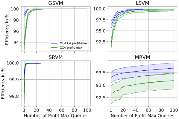
Figure 4: Efficiency of adding additionally $Q^{\textrm{P-Max}}=100$ profit-max bids in SATS for ML-CCA and CCA after 100 clock bids and 100 raised clock bids. Averaged over 100 runs including a bootstrapped 95% CI.

Path Plots of Clearing Error and Linear Item Prices

In Figures 5, 6, 7 and 8, we present for all domains in SATS the path plots for clock rounds $r=0,\ldots,100$ of the (squared) clearing error (CE) defined as:

$$\sum_{j=1}^{m}\left(\left(\sum_{i=1}^{n}x_{i}^{*}(p^{r})_{j}-c_{j}\right)^{2}\right),$$ (84)

and the linear item prices $p_{j}^{r}\in\mathbb{R}_{\geq 0}$ for $j=1,\ldots,m$.

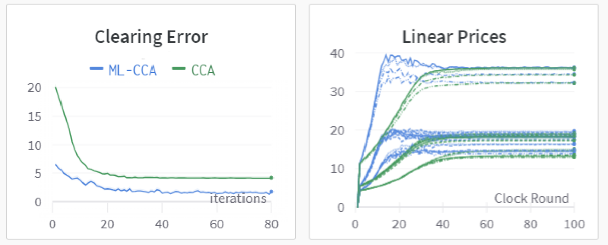
Figure 5: Left: CE of ML-CCA and CCA in GSVM per iteration (starting after the $Q^{\textrm{init}}$-phase, i.e., in clock round 20) averaged over 100 runs including the standard error. Right: linear item prices $p_{j}^{r}\in\mathbb{R}_{\geq 0}$ for $j=1,\ldots,18$ defining the demand query for each clock round $r=0,\ldots,100$ averaged over 100 runs.

In Figure 5, we present the results for GSVM. We observe that, for any iteration after the initial $Q^{\textrm{init}}=20$ clock rounds, i.e., any clock round $r=20,\ldots,100$, the CE of our ML-CCA is smaller than the CE resulting from CCA. Specifically, ML-CCA has already at iteration 0 (clock round $20)$ a small CE ($\approx$ 7) whilst CCA needs approximately 20 more iterations to reach a similar CE.

Moreover, from the path plots of the prices we can distinguish the two phases of our proposed ML-CCA: the initial CCA phase with a predefined fixed price increment in case of over-demand for the first $20$ clock rounds (or $50$ in the case of MRVM), and the ML-powered demand query generation phase starting with the $21\textsuperscript{th}$ (or $51\textsuperscript{th}$ for MRVM) clock round. We observe that our approach, for the price of each item, is immediately searching in a local neighbourhood around the plateaued CCA price of that item, and tries to clear the market by slightly increasing and decreasing certain prices. Finally, we can see that CCA properly plateaus to final CCA prices around clock rounds $80-100$, where no item is over-demanded anymore.

In Figure 6, we present the results for LSVM. We can see that for any iteration after the initial $Q^{\textrm{init}}=20$ clock rounds, i.e., any clock round $r=20,\ldots,100$, the CE of our ML-CCA is significantly smaller than the CE of CCA. Specifically, CCA requires $55$ iterations (i.e., 75 clock rounds) to reach a CE comparable to what ML-CCA can achieve in the first iterations. The price path plots in LSVM display a similar picture as in GSVM. We see that ML-CCA immediately identifies the correct region after the $Q^{\textrm{init}}=20$ initial CCA prices and then tries to locally search by increasing and decreasing prices around the plateaued CCA prices, without at the same time sacrificing efficiency, as would be the case if we were to increase the price increment of CCA to reach that price area faster.

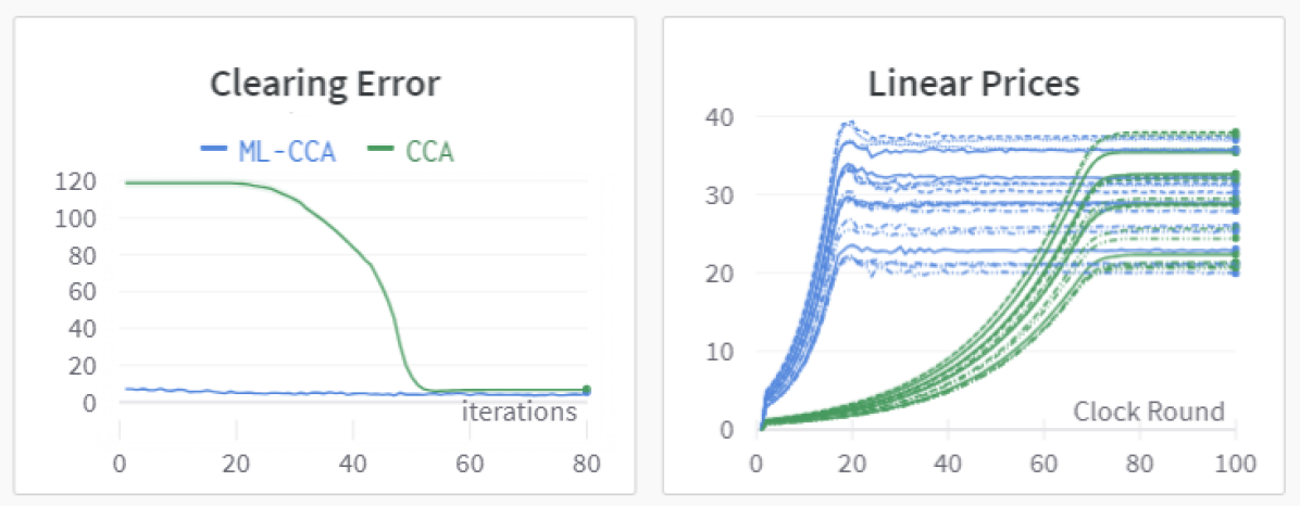
Figure 6: Left: CE of ML-CCA and CCA in LSVM per iteration (starting after the $Q^{\textrm{init}}$-phase, i.e., in clock round 20) averaged over 100 runs including the standard error. Right: linear item prices $p_{j}^{r}\in\mathbb{R}_{\geq 0}$ for $j=1,\ldots,18$ defining the demand query for each clock round $r=0,\ldots,100$ averaged over 100 runs.

In Figure 7, we present the results for SRVM on a log scale. We can see again that, for any iteration after the initial $Q^{\textrm{init}}=20$ clock rounds, i.e., any clock round $r=20,\ldots,100$, the CE of our ML-CCA is smaller than that of CCA. Furthermore, we can see that in less than $20$ iterations, our ML-CCA is able to drop the CE down to $1.1$ (with $1$ being a lower bound on the CE when clearing prices do not exist), while the CCA can never reach those numbers.

Recall, that in SRVM there are only three distinct items (i.e., $m=3$) with quantities $c_{1}=6,c_{2}=14$, and $c_{3}=9$. We again see the same behaviour of ML-CCA’s price discovery mechanism as in the other SATS domains: ML-CCA is able to immediately identify prices for the three items that are close to the final plateaued CCA prices.

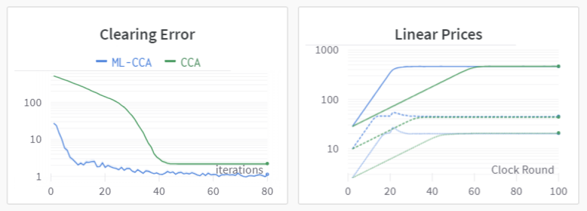
Figure 7: Left: CE of ML-CCA and CCA in SRVM per iteration (starting after the $Q^{\textrm{init}}$-phase, i.e., in clock round 20) averaged over 100 runs including the standard error. Right: linear item prices $p_{j}^{r}\in\mathbb{R}_{\geq 0}$ for $j=1,\ldots,3$ defining the demand query for each clock round $r=0,\ldots,100$ averaged over 100 runs. Both $y$-axes are on a log scale.

In Figure 8, we present the results for MRVM. Interestingly, in this domain the CCA reaches a lower CE than our ML-CCA. However, please note that CE, as defined in Equation 84, penalizes all goods equally, which can be an uninformative metric in domains where the values of different goods vary significantly. This is most pronounced in the MRVM domain, where the prices of the most valuable items are more than $100$ times larger than the prices of the least valuable goods , as shown in the right part Figure 8.

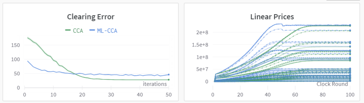
Figure 8: Left: CE of ML-CCA and CCA in MRVM per iteration (starting after the $Q^{\textrm{init}}$-phase, i.e., in clock round 50) averaged over 100 runs including the standard error. Right: linear item prices $p_{j}^{r}\in\mathbb{R}_{\geq 0}$ for $j=1,\ldots,42$ defining the demand query for each clock round $r=0,\ldots,100$ averaged over 100 runs.

D.8 Experimental Results for Reduced $Q^{\textrm{max}}=50$

	GSVM				LSVM
Mechanism	Eclock	Eraise	Eprofit	Clear	Eclock	Eraise	Eprofit	Clear
ML-CCA ($Q^{\textrm{max}}=50$)	(96.97 , 97.84 , 98.58)	(98.10 , 98.59 , 99.03)	(100.00 , 100.00 , 100.00)	51	(88.99 , 90.81 , 92.50)	(95.07 , 95.91 , 96.70)	(99.90 , 99.95 , 99.99)	17
CCA ($Q^{\textrm{max}}=50$)	(89.05 , 90.51 , 91.88)	(92.74 , 93.70 , 94.62)	(99.99 , 100.00 , 100.00)	1	(80.57 , 82.21 , 83.77)	(90.59 , 91.52 , 92.46)	(99.64 , 99.80 , 99.93)	0
CCA ($Q^{\textrm{max}}=100$)	(88.89 , 90.40 , 91.84)	(92.64 , 93.59 , 94.49)	(99.99 , 100.00 , 100.00)	3	(80.94 , 82.56 , 84.11)	(90.64 , 91.60 , 92.54)	(99.55 , 99.76 , 99.91)	0
$p$-value ($Q^{\textrm{max}}=50$)	4.2e-17	4.2e-18	0.1433	7.0e-17	2.5e-16	3.1 e-13	0.0145	9.1e-6

Table 7: Detailed results for the GSVM and LSVM domains of ML-CCA vs CCA for $Q^{\textrm{max}}=50$ including the lower and upper 95%-bootstrapped CI bounds over a test set of $100$ instances of the following metrics: E_clock = efficiency in % for clock bids, E_raise = efficiency in % for raised clock bids, E_profit = efficiency in % for raised clock bids and $100$ profit-max demand queries, Clear = percentage of instances where clearing prices were found in the clock phase. Winners for $Q^{\textrm{max}}=50$ based on a paired t-test with $\alpha=5\%$ are marked in grey. The $p$-value for this pairwise t-test with $\mathcal{H}_{0}:\mu_{\text{ML-CCA}}\leq\mu_{\text{CCA}}$ shows at which significance level we can reject the null hypothesis of CCA with $Q^{\textrm{max}}=50$ having a higher or equal average value in the corresponding metric than ML-CCA with $Q^{\textrm{max}}=50$. Additionally, we also reprint the CCA ($Q^{\textrm{max}}=100$) results from Table 5 without marking statistical significance.

	SRVM				MRVM
Mechanism	Eclock	Eraise	Eprofit	Clear	Eclock	Eraise	Eprofit	Clear
ML-CCA ($Q^{\textrm{max}}=50$)	(99.47 , 99.58 , 99.67)	(99.92 , 99.93 , 99.95)	(100.00 , 100.00 , 100.00)	13	(91.63 , 92.11 , 92.50)	(91.94 , 92.42 , 92.81)	(92.73 , 93.04 , 93.34)	0
CCA ($Q^{\textrm{max}}=50$)	(99.36 , 99.47 , 99.59)	(99.64 , 99.72 , 99.79)	(100.00 , 100.00 , 100.00)	4	(87.70 , 88.70 , 89.61)	(88.52 , 89.28 , 90.02)	(89.57 , 90.27 , 90.92)	0
CCA ($Q^{\textrm{max}}=100$)	(99.52 , 99.63 , 99.73)	(99.75 , 99.81 , 99.86)	(100.00 , 100.00 , 100.00)	8	(91.87 , 92.44 , 92.86)	(92.25 , 92.62 , 92.96)	(92.84 , 93.18 , 93.48)	0
$p$-value ($Q^{\textrm{max}}=50$)	0.088	2.9e-7	-	0.0011	2.4e-10	1.3e-12	1.6e-14	-

Table 8: Detailed results for the SRVM and MRVM domains of ML-CCA vs CCA for $Q^{\textrm{max}}=50$ including the lower and upper 95%-bootstrapped CI bounds over a test set of $100$ instances of the following metrics: E_clock = efficiency in % for clock bids, E_raise = efficiency in % for raised clock bids, E_profit = efficiency in % for raised clock bids and $100$ profit-max demand queries, Clear = percentage of instances where clearing prices were found in the clock phase. Winners for $Q^{\textrm{max}}=50$ based on a paired t-test with $\alpha=5\%$ are marked in grey. The $p$-value for this pairwise t-test with $\mathcal{H}_{0}:\mu_{\text{ML-CCA}}\leq\mu_{\text{CCA}}$ shows at which significance level we can reject the null hypothesis of CCA with $Q^{\textrm{max}}=50$ having a higher or equal average value in the corresponding metric than ML-CCA with $Q^{\textrm{max}}=50$. In all domains (including MRVM) we used $Q^{\textrm{init}}=20$ for this experiment. Additionally, we also reprint the CCA ($Q^{\textrm{max}}=100$) results from Table 6 without marking statistical significance.

In this section, we present all results of ML-CCA and CCA for a reduced number of $Q^{\textrm{max}}=50$ demand queries instead of $Q^{\textrm{max}}=100$, which were presented in the main paper in Section 6. For ease of exposition we also include the CCA optimized for $Q^{\textrm{max}}=100$ as in Section 6. We additionally present $95$% CIs and a paired t-test with $\alpha=5\%$. The $p$-value for this pairwise t-test with $\mathcal{H}_{0}:\mu_{\text{ML-CCA}}\leq\mu_{\text{CCA}}$ shows at which significance level we can reject the null hypothesis of CCA with $Q^{\textrm{max}}=50$ having a higher or equal average value in the corresponding metric than the ML-CCA with $Q^{\textrm{max}}=50$. All results are presented in Tables 7 and 8.

Just like for $Q^{\textrm{max}}=100$, our ML-CCA outperforms the CCA considerably in all domains. Specifically, the efficiency improvement after the clock phase is over $7.3$% points for GSVM, $8.6$% points in LSVM and $3.4$% points in MRVM, and all of those improvements are highly statistically significant, based on a paired t-test with $\alpha=2.4\mathrm{e}{-10}$. The two mechanisms are statistically tied in SRVM (other than for raised clock bids, where our ML-CCA again out performs the CCA). As pointed out in Section 6, this domain is very easy, and both mechanisms can solve it even with 50 clock rounds). If we add the clock bids raised heuristic of the supplementary round to both mechanisms, the efficiency improvement of ML-CCA is $4.9$% points in GSVM, $4.4$% points in LSVM and $3.1$% points in MRVM. Again all those improvements are highly significant with $\alpha=2.9\mathrm{e}{-7}$, this time also for SRVM and thus for all fur domains. Finally, it is noteworthy that in the GSVM and LSVM domains, our ML-CCA with $50$ clock rounds can achieve significantly higher efficiency with $50$ clock rounds compared to the CCA with $100$. These results even persist if we add the clock bids raised heuristic of the supplementary round to both mechanisms, which would induce up to an additional $100$ value queries for each bidder in the CCA, and only $50$ value queries for our ML-CCA.

	GSVM				LSVM
Mechanism	Eclock	Eraise	Eprofit	Clear	Eclock	Eraise	Eprofit	Clear
ML-CCA-C	(97.38 , 98.23 , 98.91)	(98.51 , 98.93 , 99.30)	(100.00 , 100.00 , 100.00)	56	(89.78 , 91.64 , 93.34)	(95.56 , 96.39 , 97.16)	(99.90 , 99.95 , 99.99)	26
ML-CCA-U	(97.05 , 97.87 , 98.56)	(98.22 , 98.67 , 99.07)	(100.00 , 100.00 , 100.00)	51	(89.84 , 91.60 , 93.28)	(95.33 , 96.16 , 96.94)	(99.90 , 99.95 , 99.99)	23
$p$-value	0.0414	0.0965	-	0.0122	0.3428	0.0189	-	0.0416

Table 9: ML-CCA with constrained $W$ (ML-CCA-C) and unconstrained $W$ minimization (ML-CCA-U). Shown are averages including the lower and upper 95%-bootstrapped CI bounds over a test set of $100$ synthetic CA instances for the GSVM and LSVM domains of the following metrics: efficiency in % for clock bids (E_clock), raised clock bids (E_raise) and raised clock bids and $100$ profit-max bids (E_profit) and percentage of instances where linear clearing prices were found (Clear). Winners based on a paired t-test with $\alpha=5\%$ are marked in grey. The $p$-value for this pairwise t-test with $\mathcal{H}_{0}:\mu_{\text{ML-CCA-C}}\leq\mu_{\text{ML-CCA-U}}$ shows at which significance level we can reject the null hypothesis of ML-CCA-U having a higher or equal average value in the corresponding metric than ML-CCA-C.

	SRVM				MRVM
Mechanism	Eclock	Eraise	Eprofit	Clear	Eclock	Eraise	Eprofit	Clear
ML-CCA-C	(99.48 , 99.59 , 99.68)	(99.92 , 99.93 , 99.95)	(100.00 , 100.00 , 100.00)	13	(92.90 , 93.12 , 93.34)	(93.03 , 93.25 , 93.47)	(93.46 , 93.67 , 93.88)	0
ML-CCA-U	(99.54 , 99.63 , 99.70)	(99.91 , 99.93 , 99.94)	(100.00 , 100.00 , 100.00)	13	(91.49 , 92.06 , 92.55)	(91.88 , 92.31 , 92.70)	(92.27 , 92.70 , 93.09)	0
$p$-value	0.7793	0.0431	-	-	9.3e-6	2.7e-08	1.0e-8	-

Table 10: ML-CCA with constrained $W$ (ML-CCA-C) and unconstrained $W$ minimization (ML-CCA-U). Shown are averages including the lower and upper 95%-bootstrapped CI bounds over a test set of $100$ synthetic CA instances for the SRVM and MRVM domains of the following metrics: efficiency in % for clock bids (E_clock), raised clock bids (E_raise) and raised clock bids plus $100$ profit-max bids (E_profit) and percentage of instances where linear clearing prices were found (Clear). Winners based on a paired t-test with $\alpha=5\%$ are marked in grey. The $p$-value for this pairwise t-test with $\mathcal{H}_{0}:\mu_{\text{ML-CCA-C}}\leq\mu_{\text{ML-CCA-U}}$ shows at which significance level we can reject the null hypothesis of ML-CCA-U having a higher or equal average value in the corresponding metric than ML-CCA-C.

D.9 Experimental Results for unconstrained $W$ minimization

In this section, we empirically evaluate the importance of constraint (9b) in the NextPrice-procedure by comparing the efficiency results of ML-CCA with constraint (9b) (ML-CCA-C) and without it (ML-CCA-U).

Constraint (9b) ensures that the predicted induced demand should constitute a feasible allocation for every clock round of ML-CCA-C, as discussed in Section 4 and Section D.6. On the other side, ML-CCA-U optimizes $W$ without any constraint (i.e., by performing unconstrained classical GD on $W$ as suggested by Lemma 2 and Theorem 3).

Those results are presented in Tables 9 and 10. In the GSVM, LSVM and SRVM domains, the results for the two approaches are almost identical (while constrained $W$ minimization is statistically better in a few cases). A noteworthy difference is that for the GSVM and LSVM domains, the unconstrained $W$ minimization clears the market in $5$% and $3$% less of the cases compared to the constrained version. Thus, as suggested in Section 4 and Section D.6, in domains where linear prices can achieve low clearing error (see Section D.7, Figures 5, 6 and 7) minimizing $W$ by performing classical GD on it without any additional constraints suffices for significant efficiency improvements compared to the CCA.

In the MRVM domain however, we can see that the efficiency improvement of performing constrained $W$ minimization compared to the unconstrained one is highly statistically significant across all three bidding heuristics with $p$-values ranging from $1.0\textrm{e}{-8}$ to $9.3\textrm{e}{-6}$. Without push bids, the efficiency improvement is approximately $1$% point. This efficiency improvement also persists if we add the clock bids raised and profit max heuristics for the supplementary round, and is again highly statistically significant. Thus, we can conclude that in all cases, there is no disadvantage to using the constrained $W$ minimization to generate the next price vector in ML-CCA. This clear improvements of ML-CCA-C over ML-CCA-U fits well our hypothesis stated in Remark 1 that constraint (9b) is especially important in cases where no LCPs exist (or when the market exhibits a high clearing error as defined in Equation 84, see Figures 5, 6, 7 and 8).