Analog simulation of high harmonic generation in atoms

Abstract

The demanding experimental access to the ultrafast dynamics of materials challenges our understanding of their electronic response to applied strong laser fields. In this work, we show that trapped ultracold atoms with highly controllable potentials can become an enabling tool to describe phenomena in a scenario where some effects are more easily accessible and twelve orders of magnitude slower. For this purpose, we characterize the mapping between the attoscience platform and atomic simulators, and propose an experimental protocol to simulate the emission yield of High Harmonic Generation, a regime that has so far been elusive to cold atom simulation. As we illustrate, the benchmark offered by these simulators can provide new insights on the conversion efficiency of extended and short nuclear potentials, as well as the response to applied elliptical polarized fields or ultrashort few-cycle pulses.

Over the last three decades, progress in laser technologies has led to significant advances in our ability to manipulate and understand electron dynamics on their natural attosecond ($10^{-18}$ s) timescale Krausz and Ivanov (2009); Salières et al. (1999); Lewenstein and L’Huillier (2009); Ciappina et al. (2017). This has triggered the development of a huge range of tools for probing and controlling matter, which includes high harmonic spectroscopy Itatani et al. (2004), laser-induced electron diffraction Zuo et al. (1996); Niikura et al. (2002), photoelectron holography Huismans et al. (2011); Figueira de Morisson Faria and Maxwell (2020), attosecond streaking Hentschel et al. (2001); Itatani et al. (2002), and reconstruction of attosecond harmonic beating by interference of two-photon transitions Paul et al. (2001); Muller (2002), to name only a small selection. One of the most prominent processes underlying some of these successes is high harmonic generation (HHG), a highly non-linear phenomenon where a system absorbs many photons of the driving laser and emits a single photon of much higher energy.

The experimental realization and interpretation of these complex processes have been guided most often by simplified theoretical descriptions that still capture the main properties of the dynamics. In the field of attoscience, simplifications such as only considering one or two active electrons, disregarding the interaction of the ionized electron with the parent ion during its propagation in the continuum, or performing saddle-point approximations have provided valuable quantitative predictions concerning HHG Amini et al. (2019); Eberly et al. (1989); Smirnova and Ivanov (2013) and other phenomena Javanainen et al. (1988); Paulus et al. (1994); Lewenstein et al. (1995); Goreslavskii et al. (2001). Additional experimental regimes do, however, require a more complete description of the system, including those where multielectronic processes Smirnova and Ivanov (2013), or Coulomb nuclear potentials play a key role Popruzhenko and Bauer (2008) (see Refs. Popruzhenko (2014); Figueira de Morisson Faria and Maxwell (2020) for reviews). This has motivated an intense development of analytical and numerical methods aimed to push current computing capabilities.

To circumvent this computation complexity, analog simulation has become an enabling tool to access phenomena with highly controllable devices, whose temporal and spatial scales are more favourable to measure than those naturally present in attosecond physics Blatt and Roos (2012); Bloch et al. (2012); Cirac and Zoller (2012). This provides an important bridge between experiments and theory, offering experimental access to complex systems that can only be theoretically approximated, while giving more external control and accessibility than the real physical system. Experimental advances in the engineering of interactions now foster the simulation of quantum chemistry phenomena, such as molecular geometries Argüello-Luengo et al. (2019); Lühmann et al. (2015), vibronic calculations Shen et al. (2018); MacDonell et al. (2021), or the presence of conical intersections Valahu et al. (2022). Recently, this experimental benchmark of chemistry processes has accessed the response of an atomic system to strong pulses Dum et al. (1998); Arlinghaus and Holthaus (2010); Senaratne et al. (2018) in the regime where the energy imparted by the simulated laser field is strong enough to ionize the target atoms, as proposed by Sala et al. Sala et al. (2017). In this work, we show that current atomic platforms now offer the unique opportunity to also simulate the relevant regime of HHG. While this has remained technically elusive for recent analog experiments where the incoming field is simulated by a shaken potential Senaratne et al. (2018), here we show how the HHG regime can in fact be accessed and measured in current platforms that offer controllable Zeeman and Stark shifts.

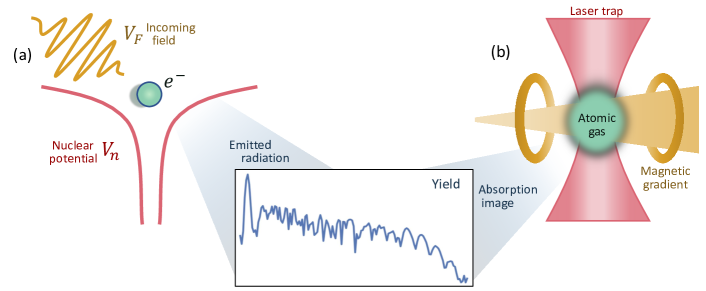
Figure 1: Schematic representation of HHG in atoms (a), and the proposed analog simulator (b). In (a) an ultrafast incoming field (brown) accelerates an electron (green), that is originally trapped by the nuclear Coulomb potential of the atom (red). The resulting oscillation of the charge emits radiation of characteristic harmonic frequencies (inset in blue). The same emission yield can be simulated on the simulator (b), where the characteristic frequencies are retrieved through absorption images of an atomic gas (green) that is trapped by a laser potential (red), and addressed by an external magnetic gradient that is tuned over time (brown).

The text is structured as follows. In Sec. I, we discuss the status of current investigation in attosecond science and motivate the different regimes that result from the frequency and strength of the laser field that drives the process. In particular, we introduce the regime of HHG, and some of its distinctive features. Sec. II presents current applications of analog quantum simulation, focusing our attention on the flexibility offered by atomic systems subjected to tunable light fields. There, we introduce an atomic simulator capable of mimicking the dynamics of an electron exposed to a strong oscillatory laser field, and derive a mapping between the experimental parameters of the simulator and the relevant units encountered in attosecond science. We also devise a protocol to access the simulation of the emission yield in HHG, highlighting the range of parameters where this correspondence is valid. As an illustrative example, we show how one can use the simulator to study the effect that short pulses and the ellipticity of the incoming field have on the efficiency of HHG. Sec III further presents details on the experimental choice of atomic species and laser pulses that are needed to simulate specific targets of common studies in attosecond science, and discuss the main sources of errors that the experimental implementation would encounter, which we numerically benchmark. In Sec. IV, we present an outlook of the venue for exploration that the proposed simulator opens.

I Introduction to HHG

HHG stands as one of the most paradigmatic examples of strong-laser field physics Krausz and Ivanov (2009); Lewenstein and L’Huillier (2009); Amini et al. (2019). HHG is a highly nonlinear optical process in which a target gets subjected to a very intense ($I\sim 10^{13}-10^{14}$ W/cm²), and often short ($\tau\sim 5-100$ fs) laser pulse, which typically belongs to the infrared regime ($\lambda\sim 700$ nm$-5$ $\mu$m). As a result, the oscillating electron emits harmonics that could extend over frequencies hundreds of orders higher than the original driving field. The unique characteristics of HHG, including coherence, ultrashort duration and high intensity, make it an exceptional source of extreme ultraviolet (XUV) radiation Drescher et al. (2001); Silva et al. (2015) and, nowadays, it configures the workhorse for the generation of attosecond pulses Krause et al. (1992a); Popmintchev et al. (2012). Consequently, HHG finds applications in various fields such as non-linear XUV optics Kobayashi et al. (1998); Midorikawa et al. (2008); Chatziathanasiou et al. (2017); Tsatrafyllis et al. (2016); Bergues et al. (2018); Nayak et al. (2018); Senfftleben et al. (2020); Orfanos et al. (2020), attosecond science Krausz and Ivanov (2009); Amini et al. (2019), molecular tomography Itatani et al. (2004) and high-resolution spectroscopy Gohle et al. (2005); Cingöz et al. (2012); Silva et al. (2018); Alcalà et al. (2022).

Although HHG is a process that has been observed in many different targets, such as atoms L’Huillier et al. (1993); Amini et al. (2019), molecules Lyngå et al. (1996), solid-state systems Ghimire et al. (2011); Goulielmakis and Brabec (2022) and nanostructures Ciappina et al. (2017), in this work we will focus on simulating HHG process in atoms. We shall now discuss the conditions required to generate high-order harmonics from atomic targets by introducing relevant parameters. The first one is the so-called multiquantum parameter $K_{0}=I_{p}/(\hbar\omega)$ Popruzhenko (2014), where $I_{p}$ is the ionization potential of the corresponding atom, and $\omega$ is the frequency of the driving field. This parameter provides an estimate of the minimal number of photons required to ionize the electron from the atomic ground state. Here, we are particularly interested in the low-frequency limit, where $K_{0}\gg 1$, indicating that ionization requires a significant number of photons. Furthermore, whether a multiphoton absorption process occurs or not also depends on the amplitude $F_{0}$, of the applied field. This motivates the introduction of the Keldysh parameter $\gamma=\sqrt{I_{p}/(2U_{p})}$ Amini et al. (2019); Popruzhenko (2014); Keldysh (1965), where $U_{p}=e^{2}\xi_{0}^{2}/(4m\omega^{2})$ is the ponderomotive energy, i.e. the average kinetic energy of an electron with mass $m$ and charge $e$ in the presence of an oscillating laser field of amplitude $\xi_{0}$ [see Fig. 1(a)].

In the case $K_{0}\gg 1$, the multiphoton regime is observed when $\gamma\gg 1$, indicating that the field only slightly perturbs the atomic potential [see Fig. 2 (a)]. The regime of interest for HHG processes corresponds to $\gamma\lesssim 1$, known as the tunneling regime, where the external field force is comparable to the atomic potential, which gets distorted and forms an effective potential barrier through which the electron can tunnel out [see Fig. 2 (b)]. Finally, and for the sake of completeness, we have the regime of over-the-barrier ionization that, typically Mulser and Bauer (2010), happens when the electric field reaches a critical value that makes the barrier maximum to coincide with the energy level of the electron ground state [see Fig. 2 (c)].

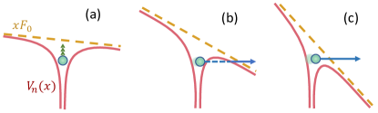
Figure 2: Schematic representation of the different ionization mechanisms at the instant of maximum tilt for different values of field strength. In (a) $\gamma\gg 1$ such that it slightly perturbs the atomic potential, potentially leading to multiphoton ionization mechanisms. In (b) $\gamma\lesssim 1$, such that the field is strong enough allowing for tunneling ionization. In (c), the electric field has reached a critical value that makes the maximum of the barrier to coincide with the energy level of the electron, leading to over-the-barrier ionization mechanism. Note that in all these cases, we are working in the regime $K_{0}\gg 1$.

Within the tunnelling regime, the three-step model, also referred to as the simple-man’s model Krause et al. (1992a); Corkum (1993); Kulander et al. (1993), provides a powerful picture of the underlying electron dynamics behind HHG. The steps within this model are as follows: the electron (i) tunnels out from the parent atom through the barrier formed by the Coulomb potential combined with the dipole interaction of the field, (ii) oscillates in the continuum under the influence of the laser electric field and, if it passes around the nucleus’ vicinity, (iii) can recombine back to the ground state emitting harmonic radiation. The energy of the emitted radiation upon recombination depends on the electronic kinetic energy at the moment of recombination and the ionization potential of the atom. However, the maximum kinetic energy that the electron can acquire from the field during its propagation is limited, leading to a natural cutoff frequency $\omega_{c}$ for the highest harmonic order in HHG, which is determined by $\hbar\omega_{c}=I_{p}+3.17U_{p}$. The nonlinear character of the HHG process can be understood from its main features, namely (i) a strong decrease in the low-order harmonics amplitude, (ii) a plateau, where the harmonic yield is almost constant, and (iii) a sudden cutoff, given by the above presented classical formula Krause et al. (1992a).

Based on the previous discussion, it is evident that the polarization character of the driving field can have significant consequences on the generated harmonic radiation. For instance, when an elliptically polarized driver is considered, the ionized electron may miss the parent ion, resulting in the absence of the recombination event Corkum (1993). This phenomenon has been extensively studied in both experimental Budil et al. (1993); Burnett et al. (1995); Weihe et al. (1995); Weihe and Bucksbaum (1996); Antoine et al. (1997); Schulze et al. (1998) and theoretical Becker et al. (1994); Antoine et al. (1996) works, demonstrating a reduced HHG conversion efficiency, i.e. the ratio between the outgoing and incoming photon fluxes, as the driving laser ellipticity increases. As an alternative strategy, a combination of two drivers that have different ellipticities and frequencies can be used to generate bright phase-matched circularly-polarized high harmonics, as shown in Refs. Milošević et al. (2000); Fleischer et al. (2014); Kfir et al. (2015); Pisanty et al. (2014); Pisanty Alatorre (2016).

While we will focus on HHG, strong laser-matter interactions can also give rise to other fascinating phenomena, including Above-Threshold Ionization (ATI) Agostini et al. (1979); Delone and Kraĭnov (2000); Milošević et al. (2006); Lewenstein and L’Huillier (2009); Agostini and DiMauro (2012) and Non-Sequential Double Ionization (NSDI) l’Huillier et al. (1983); Corkum (1993); Walker et al. (1994); Feuerstein et al. (2001); Faria and Liu (2011); Becker et al. (2012). In ATI, an electron is ionized by the strong-laser field, surpassing the ionization threshold of the corresponding atom by absorbing more photons than the ones required for ionization. The typical observable measured in ATI is the photoelectron spectrum, which exhibits distinctive peaks at electron kinetic energies separated by the energy of a single photon of the driving field Agostini et al. (1979); Milošević et al. (2006). In the non-perturbative (tunneling) regime, these peaks form a plateau that extends over electron energies on the order of $10\,U_{p}$ Hansch et al. (1997); Milošević et al. (2006). On the other hand, NSDI occurs when an ionized electron undergoes rescattering with its parent ion, resulting in the ionization of a second electron. This phenomenon is reflected in the ion yield, which exhibits a knee structure at a specific intensity threshold. The presence of this distinctive feature signifies a sudden change in the energy distribution of the emitted electron pairs, indicating a transition from sequential to non-sequential ionization processes l’Huillier et al. (1983); Walker et al. (1994).

Here, we demonstrate the capability of analog simulators to accurately replicate the key characteristics of the HHG processes in atoms. Specifically, it recovers the main features of a typical HHG spectrum –a plateau extending for few harmonic orders followed by a cutoff– with an harmonic yield that reduces for increasing values of the ellipticity. We study how the conversion efficiency of the harmonics depends on the values of $K_{0}$ and $\gamma$, and discuss how the simulated spectrum can be measured in practice for analog simulators, also providing estimates on relevant quantities towards feasible experimental implementations.

II Analog quantum simulation

The numerical simulation of chemical problems generally requires to describe many electrons that interact with external fields, the nuclei, and among themselves through Coulomb interactions. Even if one considers the nuclear positions fixed due to their larger mass (the Born-Oppenheimer approximation Born and Oppenheimer (1927); Atkins and Friedman (2015)), this is an extremely challenging task, as the associated Hilbert space grows exponentially with the number of electrons.

Over the last few decades, an alternative route to study electronic problems has emerged, based on using quantum devices that can better capture the complexity of the system. This idea was first proposed by Feynman as a way of preventing the exponential explosion of resources of quantum many-body problems Feynman (1982), and later formalized by Lloyd Lloyd (1996). Complementary to current efforts in digital simulation Arrazola et al. (2021); Arute et al. (2019); GOOGLE AI QUANTUM AND COLLABORATORS et al. (2020) (where the problem is first encoded as qubits and gates addressed by a general-purpose quantum device), simulators based on ultracold atoms have become an enabling tool, already addressing quantum matter phenomena that the most advanced classical computers cannot compute Choi et al. (2016); Trotzky et al. (2012).

At low temperatures, the interaction among atoms can be highly engineered with external lasers, which allows one to induce a rich variety of effective Hamiltonians on a highly controllable platform Cirac and Zoller (2012); Daley et al. (2022). Early experiments dealt with condensed matter problems Greiner et al. (2002); Jördens et al. (2008); Jaksch et al. (1998), detecting a transition between the superfluid and Mott insulating phases of effective Hubbard models. More recently, atomic simulators have experimentally addressed problems related to high-energy physics, such as Gauge theories, both in lattice geometries Schweizer et al. (2019); Görg et al. (2019); Aidelsburger et al. (2022) and the continuum Frölian et al. (2022). An exciting perspective consists on extending the benefits of analog quantum simulation to the field of chemistry and the response of atoms and molecules to external fields. Soon after the first experimental realization of bosonic gases Anderson et al. (1995); Davis et al. (1995), the mapping between degenerate atomic gases and single-electron dynamics was noticed Dum et al. (1998); Esry (1997). As compared to a real material, where many target atoms are present, here the simulated electron moves in a cleanly isolated environment. Furthermore, the typical energy-scales of these experiments are in the range of kHz-MHz, which provides a temporal magnification of the simulator, where attosecond pulses are associated to convenient timescales of $\mu$s-ms, i.e. $10^{9}\sim 10^{12}$ times slower.

Using the Kramers-Henneberger correspondence, the shaking of the optical trap can mimic the effect of an external force Sala et al. (2017); Rajagopal et al. (2017); Arlinghaus and Holthaus (2010), which has allowed for the recent experimental simulation of ATI processes using a bosonic gas of ⁸⁴Sr Senaratne et al. (2018), where the kinetic energy of the simulated ionized electrons is accessed through a time-of-flight measurement (TOFM) of the atoms emitted during the shaking. Extending this approach to the HHG regime is however challenging, as the needed inertial force is associated to strong nuclear potentials (see Appendix A), and the associated photonic spectra is neither emitted during the oscillation of neutral atoms, nor directly revealed by the TOFM. The present contribution advances the study of HHG simulation in different directions. In particular, (i) we show that the HHG process can be accessed in atomic simulator platforms where the external pulses are simulated by existing Stark and Zeeman shifts; (ii) we establish a correspondence between the experimental parameters in the simulator and the $K_{0}$ and $\gamma$ parameters conventionally used in attosecond science, presenting specific configuration associated to standard choices of atomic targets and ionizing pulses; (iii) we introduce a scheme to experimentally simulate the generated harmonic spectra through absorption measurements of the atomic gas, and characterize the main sources of error.

The simulator

Whenever multielectron processes can be neglected, the underlying physics of strong field processes can be described by a single active electron. The dynamics of this electron is dictated by the Hamiltonian

$$\hat{H}(\mathbf{r},t)=\frac{\mathbf{p}^{2}}{2m}+V_{n}(\mathbf{r})+V_{F}(\mathbf{r},t)\,,$$ (1)

which accounts for its kinetic energy, the attractive nuclear potential, and the incident laser field, respectively. Following the dipole approximation, the interaction with a laser field linearly polarized along the $\mathbf{x}$ axis writes as, $V_{F}(\mathbf{r},t)=F(t)x$, where $F(t)=F_{0}f(t)\sin\left(\omega t+\varphi\right)$ and $f(t)=\sin^{2}\left[\omega t/(2n_{c})\right]$ is the carrier-envelope for a pulse with $n_{c}$ cycles and wave phase $\varphi$. Here, $F_{0}=e\xi_{0}$ is the maximum force imparted by the field on the electron.

In this proposal, the dynamics of the electron inside the nuclear potential is simulated by an atomic Bose gas optically trapped by a laser beam, whose spatial profile can be highly engineered, even dynamically, with the use of spatial light modulators Boyer et al. (2006); McGloin et al. (2003) or digital mirror devices Muldoon et al. (2012); Ren et al. (2015). As a first experimental step for the simulator, we will consider the natural Gaussian profile of a laser beam of waist $r_{0}$ and depth $V_{0}$ in a one-dimensional system

$$V_{n}(x,r_{0})=V_{0}\exp\left[-x^{2}/(2r_{0}^{2})\right].$$ (2)

Similarly to the widely used atomic units, it becomes convenient to define the natural units of this system as $[\hbar]=[m]=[V_{0}r_{0}]=1$. In these units (that we denote as $[\cdot]$ along the text) the nuclear potential is fully characterized by the width of the trap, as it follows from the relation $[V_{0}]=[r_{0}]^{-1}$, and approximates a quantum harmonic oscillator whenever the associated zero-point motion of the oscillator is smaller than the waist of the beam, $[r_{0}]\gg 1$.

In Fig. 3(a), one can see that the simulated Gaussian potential (dashed blue line) matches at short distances ($x/r_{0}\ll 1$) the widely used soft-core nuclear potential of the form, $V_{\text{sc}}(x,r_{0})=1/\sqrt{x^{2}+r_{0}^{2}}$ (red line, see Appendix B for further details) Javanainen et al. (1988); Su and Eberly (1991). To highlight this connection between the simulator and the soft-core potential, in Fig. 3(b) we calculate the ionization energy associated with both nuclear potentials for different values of $r_{0}$, observing discrepancies smaller than $10\%$ for $[r_{0}]>1$. Focusing on the average width, $\sqrt{\left\langle x^{2}\right\rangle}$, of the ground-state, the long-range polynomial scaling of the soft-core potential leads to more extended eigenstates than the short-range Gaussian trap Collins and Merts (1988); Geltman (1977) (see inset), which can be experimentally explored by further shaping the laser beam. As compared to a real target with a fixed nuclear potential, the tunability offered by the simulator allows one to benchmark how the predictive power of conventional numerical methods is influenced by the range of the studied nuclear field. For example, this is relevant for the strong field approximation, where the Coulomb potential along the excursion time of the electron is often numerically disregarded Amini et al. (2019).

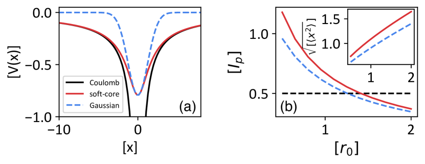
Figure 3: (a) Comparison between the Coulomb potential, $-1/|x|$ (black line), the soft-core one, $V_{\text{sc}}(x,r_{0})$ (red) and the Gaussian potential $V_{n}(x,r_{0})$ (blue) for $[r_{0}]=1$. (b) Ionization energy associated to the Gaussian and soft-core potential (same colour code as before), for different values of $r_{0}$. Black dashed line follows the Hydrogen-like condition, $[I_{p}]=0.5$. Inset indicates the average ground-state width. See Appendix C for details on the numerical calculation.

To mimic the effect of an incoming electric field under the dipole approximation, the atomic cloud is subjected to a time-dependent linear energy gradient, $V_{F}(\mathbf{r},t)$, which can be created by an optical Stark shift that is proportional to the intensity of an applied off-resonant laser field. In current platforms, a linearly-varying intensity can be created with a spatial light-modulator Choi et al. (2016), an acousto-optical device, or simply by using the slope of a Gaussian beam whose intensity and position can be dynamically adjusted. For atomic levels that are sensitive to magnetic fields, one can alternatively rely on Zeeman shifts induced by linear magnetic field gradients created and modulated with current-carrying coils Fancher et al. (2018); Lin et al. (2009); Ma et al. (2011), as represented in Fig. 1(b).

Simulation of HHG emission yield

While there is not an analog equivalent to the photons emitted during HHG, its emission yield can be accessed through the time-dependent dipole moment $d(t)=\left\langle\psi(t)\right|x\left|\psi(t)\right\rangle$, or its associated time-dependent dipole acceleration, $d_{a}(t)=\left\langle\psi(t)\right|\ddot{x}\left|\psi(t)\right\rangle$, where $\left|\psi(t)\right\rangle$ denotes the atomic state at time $t$. In HHG experiments, the spectrum of energies for photons emitted over the duration of the laser pulse is characterized by the Fourier transform, $d_{a}(\Omega)=\int dt\,d_{a}(t)e^{-i\Omega t}$ Miller (2016).

In Fig. (4) we use a time-dependent Schrödinger equation (TDSE) to calculate the dipole acceleration $d_{a}(\Omega)$ in one spatial dimension. From Fig. 3(b), we choose parameters compatible with the Hydrogen ionization potential $[r_{0}]=1.26$, so that the corresponding dissociation energy is $[I_{p}]=0.5$, and a 6-cycle pulse with an associated laser field of wavelength 800 nm and intensity $10^{14}$ W/cm². There, we see that the short-range correspondence between the soft-core (red line) and Gaussian potentials (blue) translate into a qualitative agreement of the resulting harmonic spectrum.

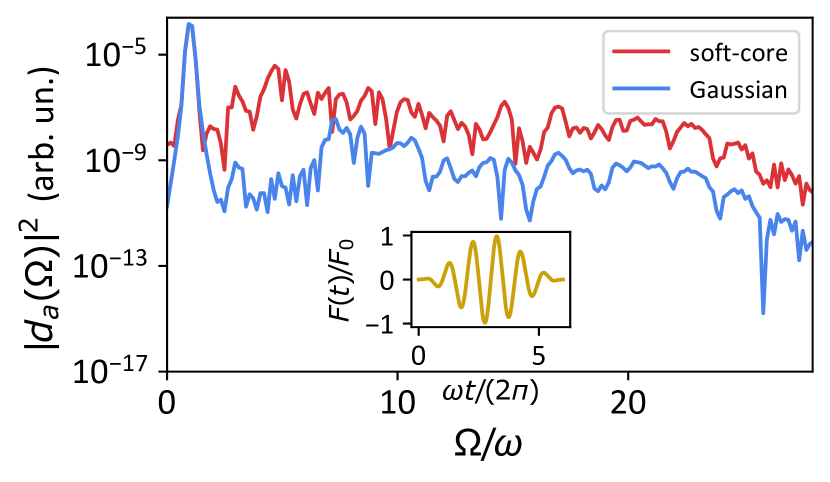
Figure 4: Simulated emission yield, $d_{a}(\Omega)$, associated to a Gaussian (blue) and soft-core potential (red line). (Inset) Sinusoidal pulse, $F(t)=F_{0}\sin^{2}(\omega t/2n_{c})\sin(\omega t)$. Parameters: $[F_{0}]=0.053$, $[\omega]=0.057$, $[r_{0}]=1.26$, and $n_{c}=6$. See Appendix C for details on the numerical calculation.

To access this quantity in the simulator, one option consists on measuring the atomic spatial density and following the Ehrenfest theorem Gordon and Kärtner (2005)

$$d_{a}(t)=-\left\langle\psi(t)\right|\nabla V_{n}(x)\left|\psi(t)\right\rangle\,,$$ (3)

where $\nabla V_{n}(x,r_{0})$ denotes the gradient of the trapping potential. For the Gaussian trap expressed in Eq. (2), this gradient can be approximated as, $\nabla_{x}V_{n}(x,r_{0})\propto V_{n}(x+r_{0}/\sqrt{2},r_{0}/\sqrt{2})-V_{n}(x-r_{0}/\sqrt{2},r_{0}/\sqrt{2})\,.$ Therefore, an absorption measurement allows one to access $d_{a}(t)$ by quantifying the asymmetry in the atomic population for positions at a characteristic separation $r_{0}/\sqrt{2}$ from the center of the trap. By repeating the measurement at different times, one can recover the emission spectrum by Fourier transforming $d_{a}(t)$.

As an alternative, one can also access the time-dependent dipole velocity, $d_{v}(t)=\left\langle\psi(t)\right|\dot{x}\left|\psi(t)\right\rangle\,,$ whose spectra is related to the emission yield as, $d_{v}(\Omega)=id_{a}(\Omega)/\Omega$, in the case of finite pulses Baggesen and Madsen (2011). Interestingly, the velocity components of the atomic cloud at a given time can be conveniently accessed in the simulator through a TOFM, where the nuclear trap is suddenly released and the gas expands ballistically. Once the gas has expanded for a time $\tau$ beyond the initial size of the cloud, the velocity component, $v$, of the state of interest is associated to an absorption detection of the cloud at a distance $x=v\tau$ from the initial trap. Given than these separations are much larger that the size of the original cloud, this approach improves the accuracy of the reconstructed emission yield for a given spatial resolution.

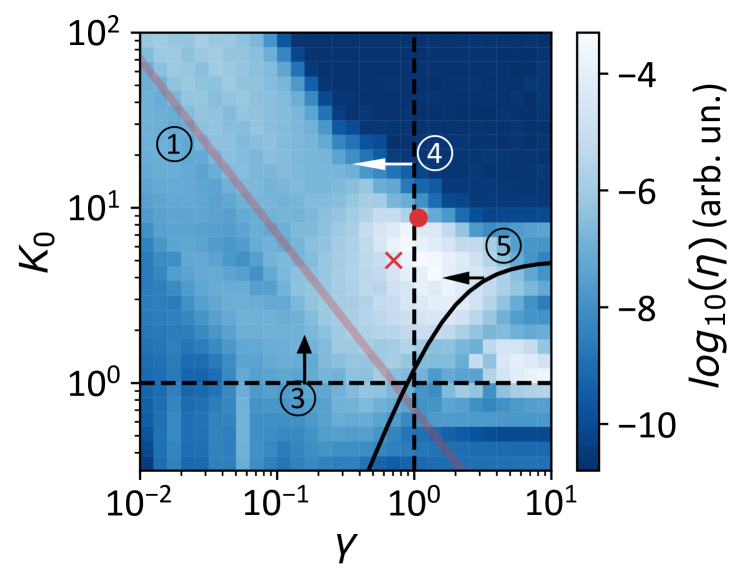
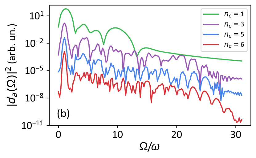
Figure 5: (a) Conversion efficiency, $\eta$, of the 5th harmonic for the Gaussian potential in Fig. 4, a six-cycle pulse ($n_{c}=6$), and different values of Keldysh ($\gamma$) and multiquantum parameter ($K_{0}$). Red line ① follows the region where a higher efficiency is expected from Eq. (6), dashed lines ③ and ④ describe the HHG region ($K_{0}\geq 1$ and $\gamma\leq 1$, respectively). ⑤ follows the frontier where the selected harmonic is below the cutoff frequency in Eq. 5. The dipole approximation ②, associated to the upper bound in Eq. (7), lies above the represented range of values for $K_{0}$. Arrows point towards the region of validity for each of these conditions. Circled red marker indicates the Gaussian configuration in Fig. 4, while the crossed marker indicates the point $K_{0}=6.31$ and $\gamma=0.81$, associated to $[F_{0}]=0.171$ and $[\omega]=0.108$. The simulated emission spectrum of the latter configuration is illustrated in panel (b) for incoming pulses with number of cycles running from $n_{c}=6$ (red) to $n_{c}=1$ (green). To improve visibility, an arbitrary vertical shift between the curves has been applied.

In Fig. 5(a) we calculate the conversion efficiency Gkortsas et al. (2011)

$$\eta=\int_{\Omega-1}^{\Omega+1}|d_{a}(\omega)|^{2}d\omega/|F_{0}|^{2}\,,$$ (4)

for one of the harmonics in the plateau region, a fixed nuclear potential $[I_{p}]=0.5$, and different values of $[\omega]=[I_{p}]/K_{0}$ and $[F_{0}]=\sqrt{2[I_{p}]^{3}}/(K_{0}\gamma)$. In order to interpret the observed regimes, both $K_{0}$ and $\gamma$ describe a complete set of parameters that characterizes the response of the simulated system to the oscillatory field. For example, expressed in natural units, the last harmonic $\Omega_{c}=\omega_{\text{c}}/\omega$ that becomes accessible below the cutoff energy writes as

$$\Omega_{c}=K_{0}\left(1+3.17/\gamma^{2}\right)\,.$$ (5)

As expected, a higher yield appears above the continuous line ⑤ where the condition, $\Omega\leq\Omega_{c}$, is satisfied.

To enhance the conversion efficiency, it is also desirable not to be too deep in the tunneling regime. An optimal situation occurs when the maximum tilt of the nuclear potential, $F_{0}r_{0}$, is comparable to $I_{p}$

$$\gamma K_{0}\approx\sqrt{[I_{p}]}[r_{0}]^{1/2},$$ (6)

and we observe that the region of largest conversion efficiency follows this heuristic scaling (red line ①).

Regarding the mapping to attoscience, the dipole approximation followed in Eq. (1) requires that the magnetic component of the incoming field can be disregarded. This imposes an upper bound ② on the intensity of the field, which writes as Reiss (2008)

$$K_{0}/4\ll\gamma^{2}[c]\,.$$ (7)

Preventing relativistic velocities on the accelerated particle ($U_{p}\ll mc^{2}$) also induces a lower-bound on the Keldysh parameter

$$\sqrt{[I_{p}]}\ll\gamma[c]\,,$$ (8)

which is less demanding than the dipole approximation along this region of greatest conversion efficiency in Eq. (6) for $\gamma\ll 1$. In the natural units of the simulator, one can see that $[c]\sim 10^{11}$ for the parameters studied in Fig. 5(a), which places this upper bound above the represented range of values for $K_{0}$.

One should note that the harmonic radiation measured in in actual attoscience HHG experiment results from a collective phenomena, involving $10^{10}\sim 10^{12}$ atoms that emit coherent radiation in phase. When comparing theory and experiment, it is therefore mandatory to include macroscopic propagation effects, which is a formidable computational task that is only addressed by a limited number of models Gaarde et al. (2008). In this simulator, however, all atoms in the bosonic gas contribute to magnify the effects manifested by a simulated single electron. The resulting harmonic spectrum is thus unaffected by the additional phase matching condition from the individual emitters that is often encountered in attosecond science experiments, providing a clean access to the simulated single-atom dipole acceleration. Furthermore, the more favourable energy, spatial and temporal scales in the simulator offer a benchmark that is less affected by the energy resolution, the uncertainty in the laser intensity and duration, or the limited dynamic range of spectroscopic measurements in ultrafast experiments Mulser and Bauer (2010).

The high tunability of the induced incoming pulse is also one of the advantages of the simulator, as compared with the fast high-intensity lasers that are typically needed in attoscience. For example, this allows one to easily simulate the response of the system to ultrashort pulses, a configuration that is otherwise demanding to access in real attosecond experiments. In Fig. 5(b), we show the simulated emission yield for pulses with different number of cycles. As the pulses get shorter, we observe that the plateau structure vanishes and the last harmonics disappear, even though the theoretical cutoff frequency $\omega_{c}$ only depends on the ionization energy and ponderomotive energy, which are the same for all the curves. Intuitively, less interference processes can take place when the number of cycles of the pulse decreases, which reduces the number of harmonics that are visible on the emission spectrum as one approaches $n_{c}=1$ (green line). Focusing on this latter case, in Fig. 6 we simulate the response of the system to a single-cycle pulse ($n_{c}=1$), for different values of $K_{0}$ and $\gamma$. When focusing on one of the lowest harmonics (the 5th one), we observe that the region of largest emission still remains well described by the different conditions introduced in Fig. 5(a).

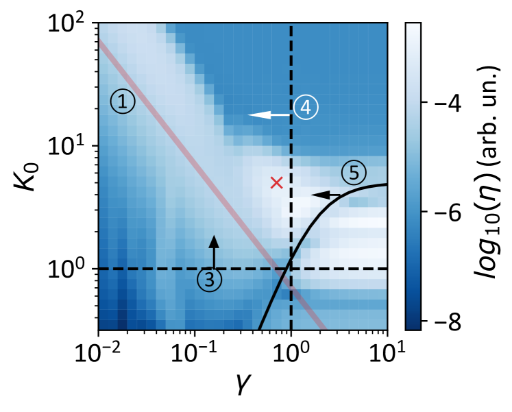
Figure 6: Conversion efficiency, $\eta$, of the 5th harmonic for the Gaussian potential in Fig. 4, a single-cycle pulse, $n_{c}=1$, and different values of Keldysh ($\gamma$) and multiquantum parameter ($K_{0}$). Red line ① follows the region where a higher efficiency is expected from Eq. (6), dashed lines ③ and ④ describe the HHG region ($K_{0}\geq 1$ and $\gamma\leq 1$, respectively). ⑤ follows the frontier where the selected harmonic is below the cutoff frequency in Eq. 5. Arrows point towards the region of validity for each of these conditions. The crossed marker indicates the point $K_{0}=6.31$ and $\gamma=0.81$, whose emission spectrum is depicted in green in Fig. 5(b).

In addition to the linearly polarized fields considered so far, the simulator also allows one to induce oscillations in a second axis, $F_{x(y)}=F_{0x(0y)}f(t)\sin\left[\omega t+\varphi+(\pi/2)\right],$ when we extend the systems to two dimensions. By controlling the ratio between the two amplitudes, i.e. the ellipticity $\varepsilon=F_{0y}/F_{0x}$, one can induce elliptic [$\varepsilon\in(0,1)$] and circularly-polarized fields ($\varepsilon=1$). In HHG, the introduction of ellipticity in the laser beam leads to the deflection of the returning electron, causing it to deviate from its intended path towards the parent nucleus. This results in a decrease of the overlap between the wavepackets of the returning electron and the initial bound state, as it has been experimentally observed Budil et al. (1993). In Fig. 7 we calculate the change in the conversion efficiency of different harmonics as we change from a linear field ($\varepsilon=0$) to elliptically-polarized field. As expected, we observe a decline in the intensity of harmonics as the ellipticity of the laser beam increases, which is more pronounced for the lowest harmonics.

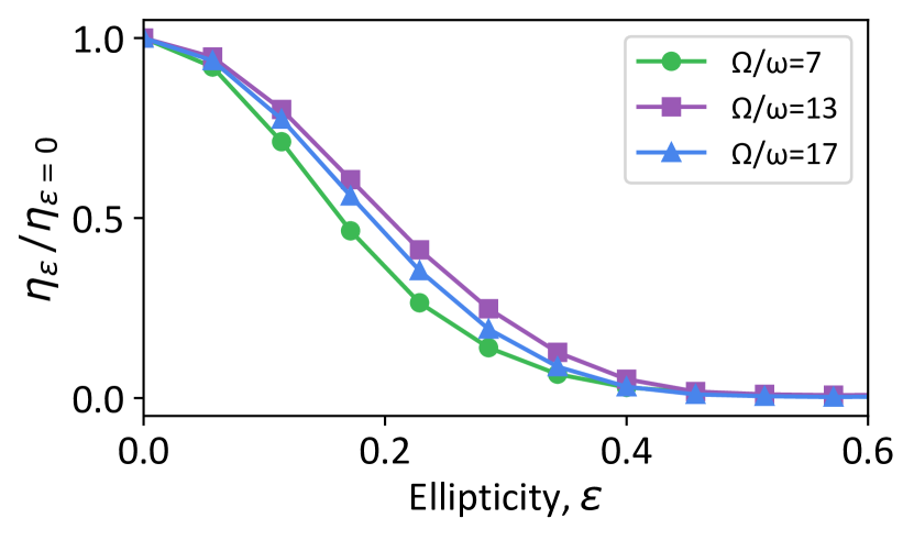
Figure 7: Conversion efficiency of different harmonics (see legend) in a 2D simulator along the x-axis, as a function of the ellipticity of the incoming field. For each harmonic, the efficiency is normalized by the value at $\varepsilon=0$. Parameters as in Fig. 4, now with a 2D Gaussian nuclear potential.

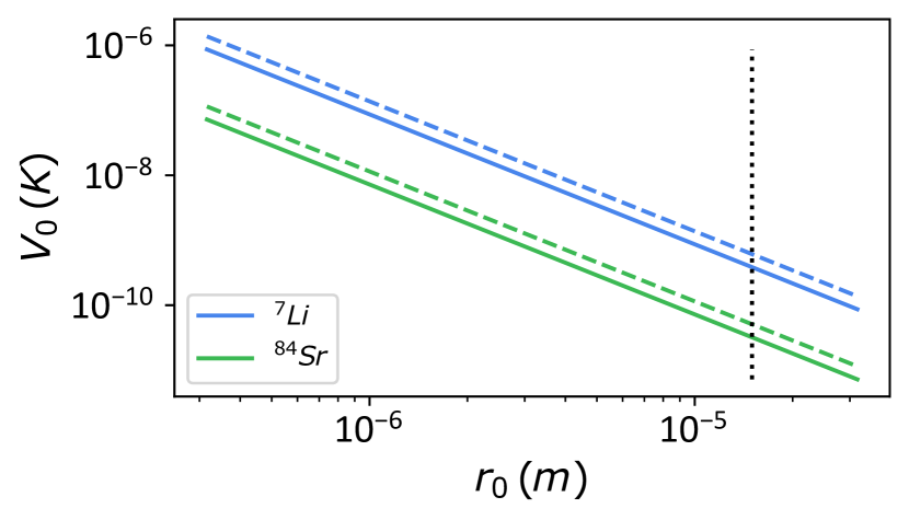
Figure 8: Nuclear potential strength, $V_{0}$ as a function of the width of the beam, $r_{0}$, following Eq. (9). Green and blue continuous lines correspond to ⁸⁴Sr and ⁷Li, respectively, for $[I_{p}]=0.5$ (continuous line) and $[I_{p}]=0.19$ (dashed line). Dotted line shows the condition $r_{0}=15\,\mu m$ of Ref. Senaratne et al. (2018).

III Experimental implementation

At this point, it is worth exploring the feasibility of the experimental parameters associated to this implementation. For a fixed geometry $[r_{0}]=1.26$ (associated to $[I_{p}]=0.5$) the needed nuclear potential scales as

$$V_{0}=\frac{\hbar^{2}}{mr_{0}^{2}}[r_{0}]\,.$$ (9)

In the case of ⁸⁴Sr and a Gaussian beam with waist $r_{0}=1\,\mu$m, the configuration $K_{0}=6.31$ and $\gamma=0.81$ [illustrated in Fig. 5(b)] corresponds to parameters, $F_{0}=1.55\cdot 10^{-26}\,$N, $\omega=94.7\,\text{Hz}$, and $V_{0}=7.22\,\text{nK}\cdot k_{B}$. Using moderate conditions of 1 Watt of 532 nm light shaped to give a linear intensity gradient across a 100 $\mu$m $\times$ 100 $\mu$m area, it is possible achieve the needed values of $F_{0}$ for ⁸⁴Sr atoms, and even produce forces two orders of magnitude stronger. However, one can observe that the associated trap depth $V_{0}\sim 10\,$nK, is well below the trap depth of around $10\,\mu$K used in previous attoscience simulators with Sr Senaratne et al. (2018).

The trap depth sets an upper limit to the temperature of atomic clouds that can be trapped by the laser potential. In order to increase the range of allowed temperatures for the experiment, Eq. (9) indicates that more relaxed cooling conditions would benefit from choosing narrower beams and lighter atomic species. This is the case of ⁷Li and $r_{0}\sim 1\,\mu$m, where the parameters needed to simulate the same attoscience configuration are: $F_{0}=1.86\cdot 10^{-25}\,$N, $\omega=1.14\,\text{kHz},$ and $V_{0}=0.87\,\mu\text{K}\cdot k_{B}$. The associated critical temperature is then consistent with state-of-the-art experiments Pollack et al. (2009). As mentioned in the previous section, for magnetic ground states, the oscillatory force can be applied by a tunable magnetic field gradient. In the case of the $|m_{F}|=2$ hyperfine state of ⁷Li, easily-attainable gradients of 50 G/cm translate into the needed range of forces $F_{0}$, or even one order of magnitude larger.

In Fig. 8, we show the scaling of the trap depth with the beam waist for ⁸⁴Sr (green) and ⁷Li (blue lines). We also show that more relaxed cooling conditions would appear in the simulation of weaker ionization energies, as we illustrate with dashed lines for the Sodium first ionization energy, $[I_{p}]=0.19$. Depending on the choice of atomic species and width of the trap, we observe a range of 3 orders of magnitude on the associated trap depth, which illustrates the flexibility that these simulators offer to access the regime of interest.

Further experimental considerations

The reconstruction of the dipole acceleration is also affected by experimental imperfections and limitations that need to be accounted for. Here, we numerically benchmark the main sources of error for the previous configuration $K_{0}=6.31$, $\gamma=0.81$ and $n_{c}=6$, where a larger conversion efficiency is expected [crossed marker in Fig. 5(a)]. To quantify the effect of these imperfections, we calculate the relative error in the determination of the local maxima of the spectra for frequencies below the cutoff frequency, which we highlight with orange dotted markers along Figs. 9-12.

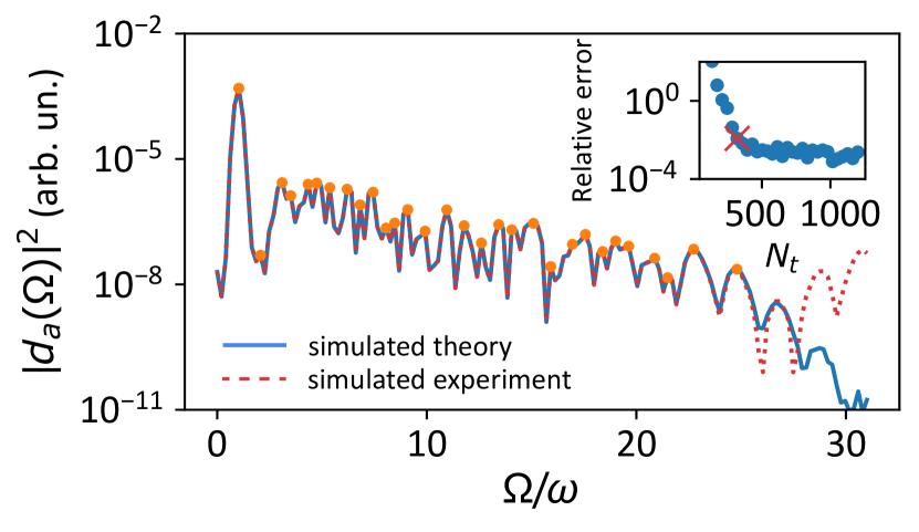
Figure 9: (Inset) Relative error of the local maxima of the dipole acceleration as a function of the number of time slots $N_{t}$ (uniformly distributed along the duration of the pulse) used in the discrete Fourier transformation. Red cross corresponds to $N_{t}=700$ divisions and the associated yield is shown in the Main Figure with red dotted line, as compared to the simulated dipole acceleration (blue line). Orange dots indicate the positions of local maxima before the cutoff energy. Parameters as in Fig. 5(b). See Appendix C for details on the numerical calculation.

In the experiment, the time-dependent dipole acceleration is measured at a finite set of times, $d_{a}(t_{n})_{n=1\ldots N_{t}}$. The accuracy of the discrete Fourier transform

$$d_{a}(\Omega)=\frac{1}{N_{t}}\sum_{n=1}^{N_{t}}d_{a}(t_{n})e^{i\Omega t_{n}}\,,$$ (10)

then depends on the number of time points used in the reconstruction, that we consider to be uniformly distributed along the duration of the pulse. In the inset of Fig. 9, we calculate the relative error in the local maxima of the emission yield for different values of temporal divisions. We observe that moderate number of time intervals $N_{t}\sim 300$ provide an error of $\sim 1\%$ that is enough to resolve the cutoff energy (see red dashed line in Fig. 9).

Experimental errors in the time points used to measure, $\Delta t_{n}=|t_{\text{meas}}-t_{n}|$, would also manifest in the reconstructed yield. In the inset of Fig. 10, we calculate the relative error in the local maxima of the emission yield for different values of noise with standard deviation $\Delta t$ around the time intervals $t_{n}$. We observe that moderate values $\omega\cdot\Delta t\sim 10^{-3}$ provide an overall relative error $\sim 10\%$ in the local maxima that is enough to resolve the cutoff energy (see red dotted line in Fig. 10). Expressed in experimental units, this translates into a correct control of time in the order of $\sim 10\,\mu$s. Overall, we see that the highest harmonics are the most sensitive ones to errors in the timing and number of time intervals, as they need to capture the rapidly oscillating response of the emission spectrum.

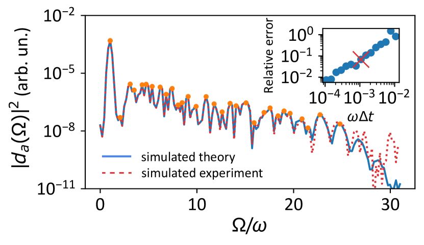
Figure 10: (Inset) Relative error of the local maxima of the dipole acceleration as a function of the standard deviation, $\Delta$, of the time points used in the discrete Fourier transformation. Red cross corresponds to $\omega\delta t\sim\cdot 10^{-3}$ and the associated yield is shown in the Main Figure with red dotted line, as compared to the simulated dipole acceleration (blue line). Orange dots indicate the positions of local maxima before the cutoff energy.

To quantify the time-dependent dipole acceleration from absorption measurements one also needs to characterize the needed accuracy on the determination of $d_{a}(t)$. In the inset of Fig. 11, we calculate the relative error in the local maxima of the emission yield for different values of relative error in the measurement of the time-dependent dipole acceleration, $\Delta d_{a}(t)/\overline{d_{a}}$, where $\overline{d_{a}}=\int_{0}^{T}|d_{a}(t)|/T$ is the temporal average over the duration of the pulse. We observe that $\Delta d_{a}(t)/\overline{d_{a}}\sim 1\%$ provides an accuracy in the emission yield that is enough to resolve the cutoff energy (see red dotted line in Fig. 11). We also observe that the highest harmonics, which have the smallest intensity, are the most affected by a limited resolution. Following the TOFM approach to access $d_{a}(t)$, typical imaging lengths, $0.1-1.0$ mm, associated to expansion times $\tau\sim 10-100$ ms Bergschneider et al. (2018), can provide the needed accuracy of $1\%$ on the retrieved velocities for an atomic cloud that has an initial width of $1-10\,\mu$m before its ballistic expansion. Also, an error in the measured density of order $\Delta|\psi|^{2}\sim 10^{-4}$ can be tolerated to reach the desired relative error of $1\%$ in the extracted time-dependent dipole (see Appendix C). As the atomic cloud spreads over its different velocity components, this results into $N_{\text{ev}}\sim 10^{6}$ single-atom events to reach the needed accuracy on velocities and atomic densities during the TOFMs used to extract each instantaneous dipole acceleration.

Taking all these demands into consideration, one can estimate the overall experimental time needed to reconstruct the time-dependent dipole acceleration. For an atomic cloud with $N_{\text{at}}\sim 10^{4}$ atoms Senaratne et al. (2018) and an estimated running time of $\tau\sim 1$ s per experiment, collecting enough statistics translates into a reasonable running time $\tau\cdot N_{\text{ev}}\cdot N_{t}/N_{\text{at}}\sim 10$ h. The major demand of resources comes from the repetition rate of the experiment and the required number of events needed to resolve the small variations in the absorption images. First experimental realizations are then especially suitable for the simulation of the first harmonics in the plateau region, as they are associated to larger conversion efficiencies, reducing the number of independent measurements that are required and, with that, the overall experimental time.

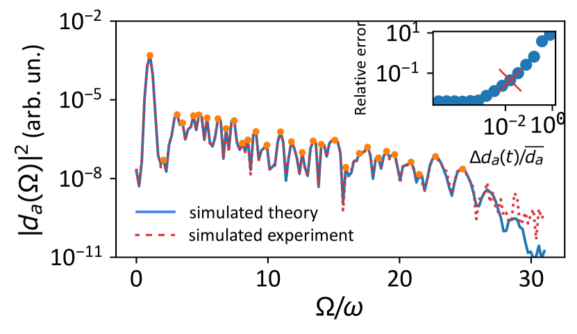
Figure 11: (Inset) Relative error of the local maxima of the dipole acceleration as a function of the error in the time points, $\Delta$, used in the discrete Fourier transformation. Red cross corresponds to $N_{\text{ev}}=5\cdot 10^{-5}$ and the associated yield is shown in the Main Figure with red dotted line, as compared to the simulated dipole acceleration (blue line). Orange dots indicate the positions of local maxima before the cutoff energy.

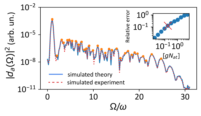
Figure 12: (Inset) Relative error of the local maxima of the dipole acceleration as a function of the interaction strength, $g$. Red cross corresponds to $[gN_{\text{at}}]=0.2$ and the associated yield is shown in the Main Figure with red dotted line, as compared to the simulated dipole acceleration (blue line). Orange dots indicate the positions of local maxima before the cutoff energy.

As a final remark, we have seen that thousands of atoms in an atomic cloud are used to simulate the state of a single electron. Atoms do, however, experience interactions at distances characterized by the scattering length, $a_{s}$. In a mean-field approach, the effect of these interactions can be described by the Gross–Pitaevskii effective Hamiltonian that depends on the atomic density at each point of space Lewenstein et al. (2012)

$$\hat{H}_{\text{int}}(\mathbf{r},t)=\hat{H}(\mathbf{r},t)+gN_{\text{at}}|\psi(\mathbf{r},t)|^{2}\,,$$ (11)

where, $g=4\pi\hbar^{2}a_{s}/m$. In the inset of Fig. 12, we calculate the relative error in the retrieved spectrum for increasing values of interaction, observing an error below $10\,\%$ for $[gN_{\text{at}}]\sim 0.2$. As compared to the previously discussed sources of error, we observe in Fig. 12 that the presence of interactions distort the entire spectrum, and not only the largest harmonics. Expressed in experimental parameters, for a gas of $N_{\text{at}}\sim 10^{4}$ atoms of ⁸⁴Sr, this value of interaction corresponds to $a_{s}=r_{0}[gN_{\text{at}}]/(4\pi N_{\text{at}}[r_{0}])\sim 10^{-12}$ m, which is three orders of magnitude shorter than the scattering length of the experiment in Ref. Senaratne et al. (2018). Using magnetic atoms such as Li, one could further rely on Feshbach resonances to engineer the required small values of scattering length Chin et al. (2010).

IV Outlook

In this work, we have shown that the HHG emission yield can be simulated in current analog experiments using atomic clouds. We have characterized the response of the simulator to elliptic potentials and short pulses, as well us the main sources of errors of experimental implementations. Based on our findings, we see that simulating attosecond dynamics by means of HHG is indeed possible with current analog simulators. Going beyond the Gaussian nuclear potential considered here, spatially modulated light can also induce extended potentials that mimic the long-range coulomb attraction that ionized electrons experience during their excursion time.

Further extensions of this platform would focus on studying the ATI phenomenon, which is also accessible in single-atoms experiments through shaken potentials. In this direction, the refined control provided by optical tweezers, can also allow one to explore multielectronic processes when each electron is mapped to an atom in the trap. Extended atom-atom repulsive interactions provided by e.g., magnetic dipoles Baier et al. (2016), Rydberg dressing Guardado-Sanchez et al. (2021); Šibalić and Adams (2018) or mediating particles Argüello-Luengo et al. (2021); Chang et al. (2018), allow one to directly tailor Coulomb corrections for a tunable degree of electronic repulsion. This offers the opportunity to simulate processes such as NSDI, where the electron-electron correlation plays a pivotal role and needs to be included in the theoretical models in order to satisfactorily describe the experimental observations Weber et al. (2000a); Moshammer et al. (2000); Weber et al. (2000b); Rudenko et al. (2007); Staudte et al. (2007). The creation of tweezer arrays of controllable geometries can also assist with the understanding of rescattering processes happening in the crystalline structure of materials Brown et al. (2022). Overall, these experiments can be of significant value to benchmark and stimulate the development of novel numerical techniques and theoretical models, helping to reach a more profound understanding of the electronic response of atoms and materials to ultrafast and intense laser fields.

Appendix A The Kramers-Henneberger correspondence

One approach to simulate an oscillatory force on the simulating atom consists in shaking the trap potential. For simplicity, let us start considering a one-dimensional system trapped in the effective potential $V_{n}(x)$. When the potential is shaken with amplitude $L$ and frequency $\omega$, the effective atomic Hamiltonian is

$$\hat{H}_{\text{lab}}(x,t)=\frac{p^{2}}{2m}+V_{n}[x+L\cos(\omega t)]\,,$$ (12)

with momenta $p$. To see the Kramers-Henneberger (KH) correspondence to an effective dipole force, one can follow the derivation in Ref. Drese and Holthaus (1997). After the unitary displacement, $U_{1}=\exp\left[-iL\cos(\omega t)p/\hbar+imL^{2}\omega\sin(2\omega t)/(8\hbar)\right]$, the rotated Hamiltonian, $H^{\prime}=U_{1}H_{\text{lab}}U_{1}^{\dagger}+i\hbar(\partial_{t}U_{1})U_{1}^{\dagger}$ writes as

$$\hat{H}^{\prime}(x,t)=\frac{\left[p-mL\sin(\omega t)\right]^{2}}{2m}+V_{n}(x)-\frac{mL^{2}\omega^{2}}{4}.$$ (13)

Performing now a momentum displacement $U_{2}=\exp\left[-imL\omega\sin(\omega t)x/\hbar\right]$ one finds the KH frame

$$\hat{H}_{\text{KH}}(x,t)=\frac{p^{2}}{2m}+V_{n}(x)+mL\omega^{2}\cos(\omega t)x-\frac{mL^{2}\omega^{2}}{4},$$ (14)

which, up to the energy shift, $mL^{2}\omega^{2}/4$, corresponds to the static Hamiltonian with an additional effective oscillating force of strength, $F_{0}=mL\omega^{2}$. In this rotated frame, the initial state $\left|\psi_{0,\text{KH}}\right\rangle=U_{2}U_{1}\left|\psi_{0}\right\rangle$, where $\left|\psi_{0}\right\rangle$ solves (12), should correspond to the bound-state of the trap, $\left|0\right\rangle$, which is also the state that can be easily prepared in the lab-frame, $\left|\psi_{0}\right\rangle=\left|0\right\rangle$. The validity of this preparation is then dictated by

$$\alpha|_{t=0}\equiv|\langle\psi_{0,\text{KH}}|\psi_{0}\rangle|=|\langle 0|U_{2}^{\dagger}U_{1}^{\dagger}|0\rangle|\sim e^{-1/\gamma^{2}}\,,$$ (15)

which makes the shaking approach specially suitable for the multiphoton ionization regime, $\gamma\gg 1$, where $\alpha\sim 1$, but challenging in the HHG regime $\gamma\lesssim 1$.

Focusing on pulses with a finite number of cycles, the field is gradually introduced by the carrier envelope, which prevents the direct mismatch derived in Eq. (15). Still, one should observe that the atomic cloud cannot follow the shaken trap if the applied gradient of the potential, $\partial_{x}V_{n}(x)$, is weaker than the simulated inertial force of interest, $F_{0}$. For the Gaussian trap in Eq. (2), this semiclassical condition writes as $V_{0}\gg F_{0}r_{0}$, which challenges the experimental realization of the region $I_{p}\sim F_{0}r_{0}$ introduced in Eq. (6), where the largest conversion efficiency of HHG is expected. This motivates the use of real oscillatory potentials to simulate this scenario, as we introduce in the main text.

Appendix B Connection to atomic units

Relevant chemical values are often expressed in atomic units (that we denote as $[[\cdot]]$): $[[\hbar]]=[[m_{e}]]=[[k_{e}]]=[[e]]\equiv 1$. Conveniently, the Bohr radius ($a_{B}$) and Hartree energy, associated to the width and energy of the ground state of atomic Hydrogen, write as

$$\left[[a_{B}]\right]=\left[\left[\frac{\hbar^{2}}{e^{2}m_{e}k_{e}}\right]\right]\equiv 1\,;\quad\left[[\text{Hartree}]\right]=\left[\left[\frac{e^{4}k_{e}^{2}m_{e}}{\hbar^{2}}\right]\right]\equiv 1\,.$$

The Hamiltonian of our simulator is of a different form, as the nuclear potential $e^{2}k_{e}/r$ is replaced by a Gaussian profile, $V_{0}\exp\left[-x^{2}/(2r_{0}^{2}\right]\approx V_{0}\left[1-x^{2}/(2r_{0}^{2})\right]$. The natural units of the system now write as

$$[\hbar]=[m]=[e]=[V_{0}r_{0}]\equiv 1\,.$$

Thus, the characteristic energy ($E_{0}$) and length scales ($a_{0}$) of the system are

$$[E_{0}]=\left[m\left(\frac{V_{0}r_{0}}{\hbar}\right)^{2}\right]\equiv 1\,,$$

$$[a_{0}]=\left[\frac{\hbar^{2}}{mV_{0}r_{0}}\right]\equiv 1\,.$$

In these units, the attoscience Hamiltonian (1) writes to lowest order (up to a constant energy shift)

$$\hat{H}\approx-\frac{\partial^{2}_{[x]}}{2}+\frac{[x]^{2}}{2[r_{0}]^{3}}+[F_{0}]\sin([\omega]t)\,[x]\,,$$

which also matches the lowest order expansion of the soft-core potential $V_{\text{sc}}(x,r_{0})$ for $[V_{0}r_{0}]=1$. The connection with the parameters of the model are thus derived as:

$$[\omega] =\omega\cdot\hbar/E_{0}\,,$$

$$[F_{0}] =F_{0}\cdot a_{0}/E_{0}\,,$$

$$[I_{p}] =I_{p}/E_{0}\,,$$

$$[c] =c\cdot\hbar/(a_{0}E_{0})\,.$$

Appendix C Numerical methods

In the simulation of Fig. 4 we consider the atomic wavefunction extended over a length $x_{\text{max}}=180\,r_{0}$, that is divided in 3000 discrete points. To prevent reflections at the edges, we apply a smooth attenuation mask of the form $\cos^{1/8}$ along the last $3r_{0}$ length of the array Krause et al. (1992b).

To solve the time-dependent Schrödinger equation, we calculate the evolution of an initial ground-state of the trapping potential, $\left|\psi(0)\right\rangle=\left|0\right\rangle$, under the time-dependent Hamiltonian (14). This evolution is Trotterized as Feit et al. (1982)

$$\begin{split}\left|\psi(t)\right\rangle&=e^{-\frac{i}{\hbar}\int_{0}^{t}H(s)ds}|0\rangle\\ &=\prod_{n=0}^{\left\lfloor t/\tau_{0}\right\rfloor}\left(e^{-\frac{i\tau_{0}}{\hbar}H_{x}(n\tau)}e^{-\frac{i\tau_{0}}{\hbar}H_{p}}\right)|0\rangle+\mathcal{O}(\tau^{2})\,,\end{split}$$ (16)

where the operators $H_{x}(t)=V(x)+F_{0}\cos(\omega t)x$ and $H_{p}=p^{2}/(2m)$ are diagonal in real and momentum space respectively, which simplifies their exponentiation by appropriately Fourier transforming the state from the real to the momentum space, where these trotterized evolution is diagonal. Along the Figures of this work, we considered $\tau_{0}\omega=0.01$.

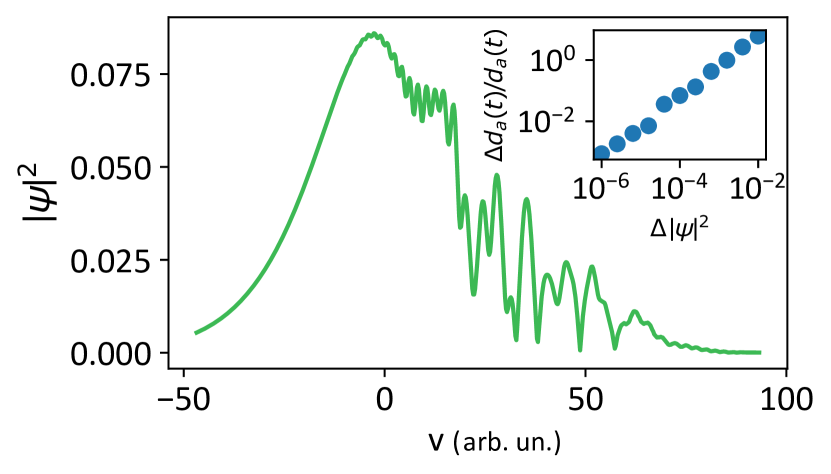
Figure 13: Velocity components of the atomic cloud, $|\psi(v)|^{2}$ after half of an incoming 6-cycle pulse is applied for the same parameters as in Fig. 5(b). (Inset) Relative error on the reconstructed dipole acceleration, $d_{a}(T/2)$ as one introduces Gaussian noise of standard deviation $\Delta|\psi|^{2}$ on the velocity components of the main Figure. Markers indicate the average over 10 random realizations.

In Fig. 13, we show the velocity components of the atomic cloud (corresponding to the squared wavefunction in momentum space) at a given instant of the driving. This curve can be measured in the experiment through TOFM, where the momenta is mapped to different positions of the atomic cloud after a ballistic expansion of the gas. In the inset, we show that the relative error of the extracted dipole acceleration scales polynomially with the noise on the atomic density detection, providing an error smaller than $1\%$ for $\Delta|\psi|^{2}\sim 10^{-4}$. This indicates a desired accuracy for experimental fluorescence measurements.

References

- Krausz and Ivanov (2009) Ferenc Krausz and Misha Ivanov, “Attosecond physics,” Rev. Mod. Phys. 81, 163–234 (2009).
- Salières et al. (1999) Pascal Salières, Anne L’Huillier, Philippe Antoine, and Maciej Lewenstein, “Study of The Spatial and Temporal Coherence of High-Order Harmonics,” in Advances In Atomic, Molecular, and Optical Physics, Vol. 41, edited by Benjamin Bederson and Herbert Walther (Academic Press, 1999) pp. 83–142.
- Lewenstein and L’Huillier (2009) Maciej Lewenstein and Anne L’Huillier, “Principles of Single Atom Physics: High-Order Harmonic Generation, Above-Threshold Ionization and Non-Sequential Ionization,” in Strong Field Laser Physics, Springer Series in Optical Sciences, edited by Thomas Brabec (Springer, New York, NY, 2009) pp. 147–183.
- Ciappina et al. (2017) M F Ciappina, J A Pérez-Hernández, A S Landsman, W A Okell, S Zherebtsov, B Förg, J Schötz, L Seiffert, T Fennel, T Shaaran, T Zimmermann, A Chacón, R Guichard, A Zaïr, J W G Tisch, J P Marangos, T Witting, A Braun, S A Maier, L Roso, M Krüger, P Hommelhoff, M F Kling, F Krausz, and M Lewenstein, “Attosecond physics at the nanoscale,” Rep. Progr. Phys. 80, 054401 (2017).
- Itatani et al. (2004) J. Itatani, J. Levesque, D. Zeidler, Hiromichi Niikura, H. Pépin, J. C. Kieffer, P. B. Corkum, and D. M. Villeneuve, “Tomographic imaging of molecular orbitals,” Nature 432, 867–871 (2004).
- Zuo et al. (1996) T Zuo, A. D. Bandrauk, and P. B. Corkum, “Laser-induced electron diffraction : A new tool for probing ultrafast molecular dynamics,” Chem. Phys. Lett. 4, 313–320 (1996).
- Niikura et al. (2002) Hiromichi Niikura, F. Légaré, R. Hasbani, A. D. Bandrauk, Misha Yu Ivanov, D. M. Villeneuve, and P. B. Corkum, “Sub-laser-cycle electron pulses for probing molecular dynamics,” Nature 417, 917–922 (2002).
- Huismans et al. (2011) Y. Huismans, A. Rouzée, A. Gijsbertsen, J. H. Jungmann, A. S. Smolkowska, P. S. W. M. Logman, F. Lépine, C. Cauchy, S. Zamith, T. Marchenko, J. M. Bakker, G. Berden, B. Redlich, A. F. G. van der Meer, H. G. Muller, W. Vermin, K. J. Schafer, M. Spanner, M. Yu. Ivanov, O. Smirnova, D. Bauer, S. V. Popruzhenko, and M. J. J. Vrakking, “Time-Resolved Holography with Photoelectrons,” Science 331, 61–64 (2011).
- Figueira de Morisson Faria and Maxwell (2020) Carla Figueira de Morisson Faria and A S Maxwell, “It is all about phases: Ultrafast holographic photoelectron imaging,” Rep. Prog. Phys. 83, 034401 (2020).
- Hentschel et al. (2001) M. Hentschel, R. Kienberger, Ch Spielmann, G. A. Reider, N. Milosevic, T. Brabec, P. Corkum, U. Heinzmann, M. Drescher, and F. Krausz, “Attosecond metrology,” Nature 414, 509–513 (2001).
- Itatani et al. (2002) J. Itatani, F. Quéré, G. L. Yudin, M. Yu. Ivanov, F. Krausz, and P. B. Corkum, “Attosecond Streak Camera,” Phys. Rev. Lett. 88, 173903 (2002).
- Paul et al. (2001) P. M. Paul, E. S. Toma, P. Breger, G. Mullot, F. Augé, Ph. Balcou, H. G. Muller, and P. Agostini, “Observation of a Train of Attosecond Pulses from High Harmonic Generation,” Science 292, 1689–1692 (2001).
- Muller (2002) H.G. Muller, “Reconstruction of attosecond harmonic beating by interference of two-photon transitions,” Appl. Phys. B 74, s17–s21 (2002).
- Amini et al. (2019) Kasra Amini, Jens Biegert, Francesca Calegari, Alexis Chacón, Marcelo F. Ciappina, Alexandre Dauphin, Dmitry K. Efimov, Carla Figueira de Morisson Faria, Krzysztof Giergiel, Piotr Gniewek, Alexandra S. Landsman, Michał Lesiuk, Michał Mandrysz, Andrew S. Maxwell, Robert Moszyński, Lisa Ortmann, Jose Antonio Pérez-Hernández, Antonio Picón, Emilio Pisanty, Jakub Prauzner-Bechcicki, Krzysztof Sacha, Noslen Suárez, Amelle Zaïr, Jakub Zakrzewski, and Maciej Lewenstein, “Symphony on strong field approximation,” Rep Prog Phys 82, 116001 (2019).
- Eberly et al. (1989) J. H. Eberly, Q. Su, and J. Javanainen, “High-order harmonic production in multiphoton ionization,” J. Opt. Soc. Am. B, JOSAB 6, 1289–1298 (1989).
- Smirnova and Ivanov (2013) O. Smirnova and M. Ivanov, “Multielectron High Harmonic Generation: simple man on a complex plane, chapter 7 in Attosecond and XUV physics, edited by T. Schultz and M. Vrakking,” (2013).
- Javanainen et al. (1988) J. Javanainen, J. H. Eberly, and Qichang Su, “Numerical simulations of multiphoton ionization and above-threshold electron spectra,” Phys. Rev. A 38, 3430–3446 (1988).
- Paulus et al. (1994) G. G. Paulus, W. Nicklich, Huale Xu, P. Lambropoulos, and H. Walther, “Plateau in above threshold ionization spectra,” Phys. Rev. Lett. 72, 2851 (1994).
- Lewenstein et al. (1995) Maciej Lewenstein, K. C. Kulander, K. J. Schafer, and P. H. Bucksbaum, “Rings in above-threshold ionization: A quasiclassical analysis,” Phys. Rev. A 51, 1495 (1995).
- Goreslavskii et al. (2001) S. P. Goreslavskii, S. V. Popruzhenko, R. Kopold, and W. Becker, “Electron-electron correlation in laser-induced nonsequential double ionization,” Physical Review A 64, 053402 (2001).
- Popruzhenko and Bauer (2008) S. V. Popruzhenko and D. Bauer, “Strong Field Approximation for Systems with Coulomb Interaction,” Journal of Modern Optics 55, 2573–2589 (2008).
- Popruzhenko (2014) S. V. Popruzhenko, “Keldysh theory of strong field ionization: history, applications, difficulties and perspectives,” J. Phys. B: At. Mol. Opt. Phys. 47, 204001 (2014).
- Blatt and Roos (2012) R. Blatt and C. F. Roos, “Quantum simulations with trapped ions,” Nature Physics 8, 277–284 (2012).
- Bloch et al. (2012) Immanuel Bloch, Jean Dalibard, and Sylvain Nascimbène, “Quantum simulations with ultracold quantum gases,” Nature Physics 8, 267–276 (2012).
- Cirac and Zoller (2012) J. Ignacio Cirac and Peter Zoller, “Goals and opportunities in quantum simulation,” Nature Physics 8, 264–266 (2012).
- Argüello-Luengo et al. (2019) Javier Argüello-Luengo, Alejandro González-Tudela, Tao Shi, Peter Zoller, and J. Ignacio Cirac, “Analogue quantum chemistry simulation,” Nature 574, 215–218 (2019).
- Lühmann et al. (2015) Dirk-Sören Lühmann, Christof Weitenberg, and Klaus Sengstock, “Emulating Molecular Orbitals and Electronic Dynamics with Ultracold Atoms,” Phys. Rev. X 5, 031016 (2015).
- Shen et al. (2018) Yangchao Shen, Yao Lu, Kuan Zhang, Junhua Zhang, Shuaining Zhang, Joonsuk Huh, and Kihwan Kim, “Quantum optical emulation of molecular vibronic spectroscopy using a trapped-ion device,” Chem. Sci. 9, 836–840 (2018).
- MacDonell et al. (2021) Ryan J. MacDonell, Claire E. Dickerson, Clare J. T. Birch, Alok Kumar, Claire L. Edmunds, Michael J. Biercuk, Cornelius Hempel, and Ivan Kassal, “Analog quantum simulation of chemical dynamics,” Chem. Sci. 12, 9794–9805 (2021).
- Valahu et al. (2022) Christophe H. Valahu, Vanessa C. Olaya-Agudelo, Ryan J. MacDonell, Tomas Navickas, Arjun D. Rao, Maverick J. Millican, Juan B. Pérez-Sánchez, Joel Yuen-Zhou, Michael J. Biercuk, Cornelius Hempel, Ting Rei Tan, and Ivan Kassal, “Direct observation of geometric phase in dynamics around a conical intersection,” (2022), arXiv:2211.07320 [quant-ph].
- Dum et al. (1998) R. Dum, A. Sanpera, K.-A. Suominen, M. Brewczyk, M. Kuś, K. Rzazewski, and M. Lewenstein, “Wave Packet Dynamics with Bose-Einstein Condensates,” Phys. Rev. Lett. 80, 3899–3902 (1998).
- Arlinghaus and Holthaus (2010) Stephan Arlinghaus and Martin Holthaus, “Driven optical lattices as strong-field simulators,” Physical Review A 81, 063612 (2010).
- Senaratne et al. (2018) Ruwan Senaratne, Shankari V. Rajagopal, Toshihiko Shimasaki, Peter E. Dotti, Kurt M. Fujiwara, Kevin Singh, Zachary A. Geiger, and David M. Weld, “Quantum simulation of ultrafast dynamics using trapped ultracold atoms,” Nat Commun 9, 2065 (2018).
- Sala et al. (2017) Simon Sala, Johann Förster, and Alejandro Saenz, “Ultracold-atom quantum simulator for attosecond science,” Physical Review A 95, 11403 (2017).
- Drescher et al. (2001) Markus Drescher, Michael Hentschel, Reinhard Kienberger, Gabriel Tempea, Christian Spielmann, Georg A. Reider, Paul B. Corkum, and Ferenc Krausz, “X-ray Pulses Approaching the Attosecond Frontier,” Science 291, 1923–1927 (2001).
- Silva et al. (2015) Francisco Silva, Stephan M. Teichmann, Seth L. Cousin, Michael Hemmer, and Jens Biegert, “Spatiotemporal isolation of attosecond soft X-ray pulses in the water window,” Nat Commun 6, 6611 (2015).
- Krause et al. (1992a) Jeffrey L. Krause, Kenneth J. Schafer, and Kenneth C. Kulander, “High-order harmonic generation from atoms and ions in the high intensity regime,” Phys. Rev. Lett. 68, 3535–3538 (1992a).
- Popmintchev et al. (2012) Tenio Popmintchev, Ming-Chang Chen, Dimitar Popmintchev, Paul Arpin, Susannah Brown, Skirmantas Ališauskas, Giedrius Andriukaitis, Tadas Balčiunas, Oliver D. Mücke, Audrius Pugzlys, Andrius Baltuška, Bonggu Shim, Samuel E. Schrauth, Alexander Gaeta, Carlos Hernández-García, Luis Plaja, Andreas Becker, Agnieszka Jaron-Becker, Margaret M. Murnane, and Henry C. Kapteyn, “Bright Coherent Ultrahigh Harmonics in the keV X-ray Regime from Mid-Infrared Femtosecond Lasers,” Science 336, 1287–1291 (2012).
- Kobayashi et al. (1998) Y. Kobayashi, T. Sekikawa, Y. Nabekawa, and S. Watanabe, “27-fs extreme ultraviolet pulse generation by high-order harmonics,” Optics Letters 23, 64–66 (1998).
- Midorikawa et al. (2008) Katsumi Midorikawa, Yasuo Nabekawa, and Akira Suda, “XUV multiphoton processes with intense high-order harmonics,” Progress in Quantum Electronics 32, 43–88 (2008).
- Chatziathanasiou et al. (2017) Stefanos Chatziathanasiou, Subhendu Kahaly, Emmanouil Skantzakis, Giuseppe Sansone, Rodrigo Lopez-Martens, Stefan Haessler, Katalin Varju, George D. Tsakiris, Dimitris Charalambidis, and Paraskevas Tzallas, “Generation of Attosecond Light Pulses from Gas and Solid State Media,” Photonics 4, 26 (2017).
- Tsatrafyllis et al. (2016) N. Tsatrafyllis, B. Bergues, H. Schröder, L. Veisz, E. Skantzakis, D. Gray, B. Bodi, S. Kuhn, G. D. Tsakiris, D. Charalambidis, and P. Tzallas, “The ion microscope as a tool for quantitative measurements in the extreme ultraviolet,” Scientific Reports 6, 21556 (2016).
- Bergues et al. (2018) B. Bergues, D. E. Rivas, M. Weidman, A. A. Muschet, W. Helml, A. Guggenmos, V. Pervak, U. Kleineberg, G. Marcus, R. Kienberger, D. Charalambidis, P. Tzallas, H. Schröder, F. Krausz, and L. Veisz, “Tabletop nonlinear optics in the 100-eV spectral region,” Optica 5, 237–242 (2018).
- Nayak et al. (2018) A. Nayak, I. Orfanos, I. Makos, M. Dumergue, S. Kühn, E. Skantzakis, B. Bodi, K. Varju, C. Kalpouzos, H. I. B. Banks, A. Emmanouilidou, D. Charalambidis, and P. Tzallas, “Multiple ionization of argon via multi-XUV-photon absorption induced by 20-GW high-order harmonic laser pulses,” Physical Review A 98, 023426 (2018).
- Senfftleben et al. (2020) B. Senfftleben, M. Kretschmar, A. Hoffmann, M. Sauppe, J. Tümmler, I. Will, T. Nagy, M. J. J. Vrakking, D. Rupp, and B. Schütte, “Highly non-linear ionization of atoms induced by intense high-harmonic pulses,” Journal of Physics: Photonics 2, 034001 (2020).
- Orfanos et al. (2020) I. Orfanos, I. Makos, I. Liontos, E. Skantzakis, B. Major, A. Nayak, M. Dumergue, S. Kühn, S. Kahaly, K. Varju, G. Sansone, B. Witzel, C. Kalpouzos, L. A. A. Nikolopoulos, P. Tzallas, and D. Charalambidis, “Non-linear processes in the extreme ultraviolet,” Journal of Physics: Photonics 2, 042003 (2020).
- Gohle et al. (2005) Christoph Gohle, Thomas Udem, Maximilian Herrmann, Jens Rauschenberger, Ronald Holzwarth, Hans A. Schuessler, Ferenc Krausz, and Theodor W. Hänsch, “A frequency comb in the extreme ultraviolet,” Nature 436, 234–237 (2005).
- Cingöz et al. (2012) Arman Cingöz, Dylan C. Yost, Thomas K. Allison, Axel Ruehl, Martin E. Fermann, Ingmar Hartl, and Jun Ye, “Direct frequency comb spectroscopy in the extreme ultraviolet,” Nature 482, 68–71 (2012).
- Silva et al. (2018) R. E. F. Silva, Igor V. Blinov, Alexey N. Rubtsov, O. Smirnova, and M. Ivanov, “High-harmonic spectroscopy of ultrafast many-body dynamics in strongly correlated systems,” Nature Photonics 12, 266–270 (2018).
- Alcalà et al. (2022) Jordi Alcalà, Utso Bhattacharya, Jens Biegert, Marcelo Ciappina, Ugaitz Elu, Tobias Graß, Piotr T. Grochowski, Maciej Lewenstein, Anna Palau, Themistoklis P. H. Sidiropoulos, Tobias Steinle, and Igor Tyulnev, “High-harmonic spectroscopy of quantum phase transitions in a high-Tc superconductor,” Proceedings of the National Academy of Sciences 119, e2207766119 (2022).
- L’Huillier et al. (1993) Anne L’Huillier, M. Lewenstein, P. Salières, Ph. Balcou, M. Yu. Ivanov, J. Larsson, and C. G. Wahlström, “High-order Harmonic-generation cutoff,” Physical Review A 48, R3433–R3436 (1993).
- Lyngå et al. (1996) C. Lyngå, A. L’Huillier, and C.-G. Wahlström, “High-order harmonic generation in molecular gases,” Journal of Physics B: Atomic, Molecular and Optical Physics 29, 3293 (1996).
- Ghimire et al. (2011) Shambhu Ghimire, Anthony D. DiChiara, Emily Sistrunk, Pierre Agostini, Louis F. DiMauro, and David A. Reis, “Observation of high-order harmonic generation in a bulk crystal,” Nature Physics 7, 138–141 (2011).
- Goulielmakis and Brabec (2022) Eleftherios Goulielmakis and Thomas Brabec, “High harmonic generation in condensed matter,” Nature Photonics 16, 411–421 (2022).
- Keldysh (1965) L Keldysh, “Ionization of atoms in an alternating electric field,” Sov. Phys. JETP 20, 1307–1314 (1965).
- Mulser and Bauer (2010) Peter Mulser and Dieter Bauer, “Intense Laser–Atom Interaction,” in High Power Laser-Matter Interaction, Springer Tracts in Modern Physics, edited by Peter Mulser and Dieter Bauer (Springer, Berlin, Heidelberg, 2010) pp. 267–330.
- Corkum (1993) P. B. Corkum, “Plasma perspective on strong field multiphoton ionization,” Physical Review Letters 71, 1994–1997 (1993).
- Kulander et al. (1993) K. C. Kulander, K. J. Schafer, and J. L. Krause, “Dynamics of Short-Pulse Excitation, Ionization and Harmonic Conversion,” in Super-Intense Laser-Atom Physics, NATO ASI Series, edited by Bernard Piraux, Anne L’Huillier, and Kazimierz Rzążewski (Springer US, Boston, MA, 1993) pp. 95–110.
- Budil et al. (1993) K. S. Budil, P. Salières, Anne L’Huillier, T. Ditmire, and M. D. Perry, “Influence of ellipticity on harmonic generation,” Phys. Rev. A 48, R3437–R3440 (1993).
- Burnett et al. (1995) N. H. Burnett, C. Kan, and P. B. Corkum, “Ellipticity and polarization effects in harmonic generation in ionizing neon,” Physical Review A 51, R3418–R3421 (1995).
- Weihe et al. (1995) F. A. Weihe, S. K. Dutta, G. Korn, D. Du, P. H. Bucksbaum, and P. L. Shkolnikov, “Polarization of high-intensity high-harmonic generation,” Physical Review A 51, R3433–R3436 (1995).
- Weihe and Bucksbaum (1996) F. A. Weihe and P. H. Bucksbaum, “Measurement of the polarization state of high harmonics generated in gases,” JOSA B 13, 157–161 (1996).
- Antoine et al. (1997) Philippe Antoine, Bertrand Carré, Anne L’Huillier, and Maciej Lewenstein, “Polarization of high-order harmonics,” Physical Review A 55, 1314–1324 (1997).
- Schulze et al. (1998) D. Schulze, M. Dörr, G. Sommerer, J. Ludwig, P. V. Nickles, T. Schlegel, W. Sandner, M. Drescher, U. Kleineberg, and U. Heinzmann, “Polarization of the 61st harmonic from 1053-nm laser radiation in neon,” Physical Review A 57, 3003–3007 (1998).
- Becker et al. (1994) W. Becker, A. Lohr, and M. Kleber, “Effects of rescattering on above-threshold ionization,” Journal of Physics B: Atomic, Molecular and Optical Physics 27, L325 (1994).
- Antoine et al. (1996) Philippe Antoine, Anne L’Huillier, Maciej Lewenstein, Pascal Salières, and Bertrand Carré, “Theory of high-order harmonic generation by an elliptically polarized laser field,” Physical Review A 53, 1725–1745 (1996).
- Milošević et al. (2000) Dejan B. Milošević, Wilhelm Becker, and Richard Kopold, “Generation of circularly polarized high-order harmonics by two-color coplanar field mixing,” Physical Review A 61, 063403 (2000).
- Fleischer et al. (2014) Avner Fleischer, Ofer Kfir, Tzvi Diskin, Pavel Sidorenko, and Oren Cohen, “Spin angular momentum and tunable polarization in high-harmonic generation,” Nature Photonics 8, 543–549 (2014).
- Kfir et al. (2015) Ofer Kfir, Patrik Grychtol, Emrah Turgut, Ronny Knut, Dmitriy Zusin, Dimitar Popmintchev, Tenio Popmintchev, Hans Nembach, Justin M. Shaw, Avner Fleischer, Henry Kapteyn, Margaret Murnane, and Oren Cohen, “Generation of bright phase-matched circularly-polarized extreme ultraviolet high harmonics,” Nature Photonics 9, 99–105 (2015).
- Pisanty et al. (2014) Emilio Pisanty, Suren Sukiasyan, and Misha Ivanov, “Spin conservation in high-order-harmonic generation using bicircular fields,” Physical Review A 90, 043829 (2014).
- Pisanty Alatorre (2016) Emilio Pisanty Alatorre, Electron dynamics in complex time and complex space, Ph.D. thesis (2016).
- Agostini et al. (1979) P. Agostini, F. Fabre, G. Mainfray, G. Petite, and N. K. Rahman, “Free-Free Transitions Following Six-Photon Ionization of Xenon Atoms,” Physical Review Letters 42, 1127–1130 (1979).
- Delone and Kraĭnov (2000) N. B. Delone and Vladimir Pavlovich Kraĭnov, Multiphoton Processes in Atoms: Second Edition (Springer Science & Business Media, 2000).
- Milošević et al. (2006) D. B. Milošević, G. G. Paulus, D. Bauer, and W. Becker, “Above-threshold ionization by few-cycle pulses,” J. Phys. B: At. Mol. Opt. Phys. 39, R203 (2006).
- Agostini and DiMauro (2012) Pierre Agostini and Louis F. DiMauro, “Chapter 3 - Atomic and Molecular Ionization Dynamics in Strong Laser Fields: From Optical to X-rays,” in Advances In Atomic, Molecular, and Optical Physics, Advances in Atomic, Molecular, and Optical Physics, Vol. 61, edited by Paul Berman, Ennio Arimondo, and Chun Lin (Academic Press, 2012) pp. 117–158.
- l’Huillier et al. (1983) A. l’Huillier, L. A. Lompre, G. Mainfray, and C. Manus, “Multiply charged ions induced by multiphoton absorption in rare gases at 0.53 um,” Physical Review A 27, 2503–2512 (1983).
- Walker et al. (1994) B. Walker, B. Sheehy, L. F. DiMauro, P. Agostini, K. J. Schafer, and K. C. Kulander, “Precision Measurement of Strong Field Double Ionization of Helium,” Physical Review Letters 73, 1227–1230 (1994).
- Feuerstein et al. (2001) B. Feuerstein, R. Moshammer, D. Fischer, A. Dorn, C. D. Schröter, J. Deipenwisch, J. R. Crespo Lopez-Urrutia, C. Höhr, P. Neumayer, J. Ullrich, H. Rottke, C. Trump, M. Wittmann, G. Korn, and W. Sandner, “Separation of Recollision Mechanisms in Nonsequential Strong Field Double Ionization of Ar: The Role of Excitation Tunneling,” Physical Review Letters 87, 043003 (2001).
- Faria and Liu (2011) Carla Figueira de Morisson Faria and X Liu, “Electron–electron correlation in strong laser fields,” Journal of Modern Optics 58, 1076–1131 (2011).
- Becker et al. (2012) Wilhelm Becker, XiaoJun Liu, Phay Jo Ho, and Joseph H. Eberly, “Theories of photoelectron correlation in laser-driven multiple atomic ionization,” Reviews of Modern Physics 84, 1011–1043 (2012).
- Hansch et al. (1997) P. Hansch, M. A. Walker, and L. D. Van Woerkom, “Resonant hot-electron production in above-threshold ionization,” Physical Review A 55, R2535–R2538 (1997).
- Born and Oppenheimer (1927) M. Born and R. Oppenheimer, “Zur Quantentheorie der Molekeln,” Annalen der Physik 389, 457–484 (1927).
- Atkins and Friedman (2015) Peter Atkins and Ronald Friedman, “An introduction to molecular structure,” in Molecular quantum mechanics (Oxford University Press, Oxford, 2015) Chap. 8, pp. 249–286.
- Feynman (1982) Richard P Feynman, “Simulating Physics with Computers,” International Journal of Theoretical Physics 217 (1982).
- Lloyd (1996) Seth Lloyd, “Universal quantum simulators,” Science 273, 1073–1078 (1996).
- Arrazola et al. (2021) J. M. Arrazola, V. Bergholm, K. Brádler, T. R. Bromley, M. J. Collins, I. Dhand, A. Fumagalli, T. Gerrits, A. Goussev, L. G. Helt, J. Hundal, T. Isacsson, R. B. Israel, J. Izaac, S. Jahangiri, R. Janik, N. Killoran, S. P. Kumar, J. Lavoie, A. E. Lita, D. H. Mahler, M. Menotti, B. Morrison, S. W. Nam, L. Neuhaus, H. Y. Qi, N. Quesada, A. Repingon, K. K. Sabapathy, M. Schuld, D. Su, J. Swinarton, A. Száva, K. Tan, P. Tan, V. D. Vaidya, Z. Vernon, Z. Zabaneh, and Y. Zhang, “Quantum circuits with many photons on a programmable nanophotonic chip,” Nature 591, 54–60 (2021).
- Arute et al. (2019) Frank Arute, Kunal Arya, Ryan Babbush, Dave Bacon, Joseph C. Bardin, Rami Barends, Rupak Biswas, Sergio Boixo, Fernando G. S. L. Brandao, David A. Buell, Brian Burkett, Yu Chen, Zijun Chen, Ben Chiaro, Roberto Collins, William Courtney, Andrew Dunsworth, Edward Farhi, Brooks Foxen, Austin Fowler, Craig Gidney, Marissa Giustina, Rob Graff, Keith Guerin, Steve Habegger, Matthew P. Harrigan, Michael J. Hartmann, Alan Ho, Markus Hoffmann, Trent Huang, Travis S. Humble, Sergei V. Isakov, Evan Jeffrey, Zhang Jiang, Dvir Kafri, Kostyantyn Kechedzhi, Julian Kelly, Paul V. Klimov, Sergey Knysh, Alexander Korotkov, Fedor Kostritsa, David Landhuis, Mike Lindmark, Erik Lucero, Dmitry Lyakh, Salvatore Mandrà, Jarrod R. McClean, Matthew McEwen, Anthony Megrant, Xiao Mi, Kristel Michielsen, Masoud Mohseni, Josh Mutus, Ofer Naaman, Matthew Neeley, Charles Neill, Murphy Yuezhen Niu, Eric Ostby, Andre Petukhov, John C. Platt, Chris Quintana, Eleanor G. Rieffel, Pedram Roushan, Nicholas C. Rubin, Daniel Sank, Kevin J. Satzinger, Vadim Smelyanskiy, Kevin J. Sung, Matthew D. Trevithick, Amit Vainsencher, Benjamin Villalonga, Theodore White, Z. Jamie Yao, Ping Yeh, Adam Zalcman, Hartmut Neven, and John M. Martinis, “Quantum supremacy using a programmable superconducting processor,” Nature 574, 505–510 (2019).
- GOOGLE AI QUANTUM AND COLLABORATORS et al. (2020) GOOGLE AI QUANTUM AND COLLABORATORS, Frank Arute, Kunal Arya, Ryan Babbush, Dave Bacon, Joseph C. Bardin, Rami Barends, Sergio Boixo, Michael Broughton, Bob B. Buckley, David A. Buell, Brian Burkett, Nicholas Bushnell, Yu Chen, Zijun Chen, Benjamin Chiaro, Roberto Collins, William Courtney, Sean Demura, Andrew Dunsworth, Edward Farhi, Austin Fowler, Brooks Foxen, Craig Gidney, Marissa Giustina, Rob Graff, Steve Habegger, Matthew P. Harrigan, Alan Ho, Sabrina Hong, Trent Huang, William J. Huggins, Lev Ioffe, Sergei V. Isakov, Evan Jeffrey, Zhang Jiang, Cody Jones, Dvir Kafri, Kostyantyn Kechedzhi, Julian Kelly, Seon Kim, Paul V. Klimov, Alexander Korotkov, Fedor Kostritsa, David Landhuis, Pavel Laptev, Mike Lindmark, Erik Lucero, Orion Martin, John M. Martinis, Jarrod R. McClean, Matt McEwen, Anthony Megrant, Xiao Mi, Masoud Mohseni, Wojciech Mruczkiewicz, Josh Mutus, Ofer Naaman, Matthew Neeley, Charles Neill, Hartmut Neven, Murphy Yuezhen Niu, Thomas E. O’Brien, Eric Ostby, Andre Petukhov, Harald Putterman, Chris Quintana, Pedram Roushan, Nicholas C. Rubin, Daniel Sank, Kevin J. Satzinger, Vadim Smelyanskiy, Doug Strain, Kevin J. Sung, Marco Szalay, Tyler Y. Takeshita, Amit Vainsencher, Theodore White, Nathan Wiebe, Z. Jamie Yao, Ping Yeh, and Adam Zalcman, “Hartree-Fock on a superconducting qubit quantum computer,” Science 369, 1084–1089 (2020).
- Choi et al. (2016) Jae-Joon Choi, Sebastian Hild, Johannes Zeiher, Peter Schauß, Antonio Rubio-Abadal, Tarik Yefsah, Vedika Khemani, David A Huse, Immanuel Bloch, and Christian Gross, “Exploring the many-body localization transition in two dimensions.” Science 352, 1547–52 (2016).
- Trotzky et al. (2012) S. Trotzky, Y-A. Chen, A. Flesch, I. P. McCulloch, U. Schollwöck, J. Eisert, and I. Bloch, “Probing the relaxation towards equilibrium in an isolated strongly correlated one-dimensional Bose gas,” Nature Physics 8, 325–330 (2012).
- Daley et al. (2022) Andrew J. Daley, Immanuel Bloch, Christian Kokail, Stuart Flannigan, Natalie Pearson, Matthias Troyer, and Peter Zoller, “Practical quantum advantage in quantum simulation,” Nature 607, 667–676 (2022).
- Greiner et al. (2002) Markus Greiner, Olaf Mandel, Tilman Esslinger, Theodor W. Hänsch, and Immanuel Bloch, “Quantum phase transition from a superfluid to a Mott insulator in a gas of ultracold atoms,” Nature 415, 39–44 (2002).
- Jördens et al. (2008) Robert Jördens, Niels Strohmaier, Kenneth Günter, Henning Moritz, and Tilman Esslinger, “A Mott insulator of fermionic atoms in an optical lattice,” Nature 455, 204–207 (2008).
- Jaksch et al. (1998) D. Jaksch, C. Bruder, J. I. Cirac, C. W. Gardiner, and P. Zoller, “Cold Bosonic Atoms in Optical Lattices,” Physical Review Letters 81, 3108–3111 (1998).
- Schweizer et al. (2019) Christian Schweizer, Fabian Grusdt, Moritz Berngruber, Luca Barbiero, Eugene Demler, Nathan Goldman, Immanuel Bloch, and Monika Aidelsburger, “Floquet approach to Z2 lattice gauge theories with ultracold atoms in optical lattices,” Nat. Phys. 15, 1168–1173 (2019).
- Görg et al. (2019) Frederik Görg, Kilian Sandholzer, Joaquín Minguzzi, Rémi Desbuquois, Michael Messer, and Tilman Esslinger, “Realization of density-dependent Peierls phases to engineer quantized gauge fields coupled to ultracold matter,” Nature Physics 15, 1161–1167 (2019).
- Aidelsburger et al. (2022) Monika Aidelsburger, Luca Barbiero, Alejandro Bermudez, Titas Chanda, Alexandre Dauphin, Daniel González-Cuadra, Przemysław R. Grzybowski, Simon Hands, Fred Jendrzejewski, Johannes Jünemann, Gediminas Juzeliūnas, Valentin Kasper, Angelo Piga, Shi-Ju Ran, Matteo Rizzi, Germán Sierra, Luca Tagliacozzo, Emanuele Tirrito, Torsten V. Zache, Jakub Zakrzewski, Erez Zohar, and Maciej Lewenstein, “Cold atoms meet lattice gauge theory,” Philosophical Transactions of the Royal Society A: Mathematical, Physical and Engineering Sciences 380, 20210064 (2022).
- Frölian et al. (2022) Anika Frölian, Craig S. Chisholm, Elettra Neri, Cesar R. Cabrera, Ramón Ramos, Alessio Celi, and Leticia Tarruell, “Realizing a 1D topological gauge theory in an optically dressed BEC,” Nature 608, 293–297 (2022).
- Anderson et al. (1995) M. H. Anderson, J. R. Ensher, M. R. Matthews, C. E. Wieman, and E. A. Cornell, “Observation of Bose-Einstein Condensation in a Dilute Atomic Vapor,” Science 269, 198–201 (1995).
- Davis et al. (1995) K. B. Davis, M. O. Mewes, M. R. Andrews, N. J. van Druten, D. S. Durfee, D. M. Kurn, and W. Ketterle, “Bose-Einstein Condensation in a Gas of Sodium Atoms,” Phys. Rev. Lett. 75, 3969–3973 (1995).
- Esry (1997) B. D. Esry, “Hartree-Fock theory for Bose-Einstein condensates and the inclusion of correlation effects,” Phys. Rev. A 55, 1147–1159 (1997).
- Rajagopal et al. (2017) Shankari V. Rajagopal, Kurt M. Fujiwara, Ruwan Senaratne, Kevin Singh, Zachary A. Geiger, and David M. Weld, “Quantum Emulation of Extreme Non-Equilibrium Phenomena with Trapped Atoms,” Annalen der Physik 529, 1700008 (2017).
- Boyer et al. (2006) V. Boyer, R. M. Godun, G. Smirne, D. Cassettari, C. M. Chandrashekar, A. B. Deb, Z. J. Laczik, and C. J. Foot, “Dynamic manipulation of Bose-Einstein condensates with a spatial light modulator,” Phys. Rev. A 73, 031402 (2006).
- McGloin et al. (2003) D. McGloin, G. C. Spalding, H. Melville, W. Sibbett, and K. Dholakia, “Applications of spatial light modulators in atom optics,” Opt. Express, OE 11, 158–166 (2003).
- Muldoon et al. (2012) Cecilia Muldoon, Lukas Brandt, Jian Dong, Dustin Stuart, Edouard Brainis, Matthew Himsworth, and Axel Kuhn, “Control and manipulation of cold atoms in optical tweezers,” New J. Phys. 14, 073051 (2012).
- Ren et al. (2015) Yu-Xuan Ren, Rong-De Lu, and Lei Gong, “Tailoring light with a digital micromirror device,” Annalen der Physik 527, 447–470 (2015).
- Su and Eberly (1991) Q. Su and J. H. Eberly, “Model atom for multiphoton physics,” Phys. Rev. A 44, 5997–6008 (1991).
- Collins and Merts (1988) L. A. Collins and A. L. Merts, “Model calculations for an atom interacting with an intense, time-dependent electric field,” Phys. Rev. A 37, 2415–2431 (1988).
- Geltman (1977) S. Geltman, “Ionization of a model atom by a pulse of coherent radiation,” J. Phys. B: Atom. Mol. Phys. 10, 831 (1977).
- Fancher et al. (2018) C. T. Fancher, A. J. Pyle, A. P. Rotunno, and S. Aubin, “Microwave ac Zeeman force for ultracold atoms,” Phys. Rev. A 97, 043430 (2018).
- Lin et al. (2009) Y.-J. Lin, R. L. Compton, K. Jiménez-García, J. V. Porto, and I. B. Spielman, “Synthetic magnetic fields for ultracold neutral atoms,” Nature 462, 628–632 (2009).
- Ma et al. (2011) Ruichao Ma, M. Eric Tai, Philipp M. Preiss, Waseem S. Bakr, Jonathan Simon, and Markus Greiner, “Photon-Assisted Tunneling in a Biased Strongly Correlated Bose Gas,” Phys. Rev. Lett. 107, 095301 (2011).
- Gaarde et al. (2008) Mette B. Gaarde, Jennifer L. Tate, and Kenneth J. Schafer, “Macroscopic aspects of attosecond pulse generation,” J. Phys. B: At. Mol. Opt. Phys. 41, 132001 (2008).
- Miller (2016) Michelle R. Miller, Time Resolving Electron Dynamics in Atomic and Molecular Systems Using High-Harmonic Spectroscopy, Ph.D. thesis, University of Colorado Boulder (2016).
- Gordon and Kärtner (2005) Ariel Gordon and Franz X. Kärtner, “Quantitative Modeling of Single Atom High Harmonic Generation,” Phys. Rev. Lett. 95, 223901 (2005).
- Baggesen and Madsen (2011) Jan Conrad Baggesen and Lars Bojer Madsen, “On the dipole, velocity and acceleration forms in high-order harmonic generation from a single atom or molecule,” J. Phys. B: At. Mol. Opt. Phys. 44, 115601 (2011).
- Gkortsas et al. (2011) Vasileios-Marios Gkortsas, Siddharth Bhardwaj, Edilson L. Falcão-Filho, Kyung-Han Hong, Ariel Gordon, and Franz X. Kärtner, “Scaling of high harmonic generation conversion efficiency,” J. Phys. B: At. Mol. Opt. Phys. 44, 045601 (2011).
- Reiss (2008) H. R. Reiss, “Limits on Tunneling Theories of Strong-Field Ionization,” Phys. Rev. Lett. 101, 043002 (2008).
- Pollack et al. (2009) S. E. Pollack, D. Dries, M. Junker, Y. P. Chen, T. A. Corcovilos, and R. G. Hulet, “Extreme Tunability of Interactions in a 7Li Bose-Einstein Condensate,” Phys. Rev. Lett. 102, 090402 (2009).
- Bergschneider et al. (2018) Andrea Bergschneider, Vincent M. Klinkhamer, Jan Hendrik Becher, Ralf Klemt, Gerhard Zürn, Philipp M. Preiss, and Selim Jochim, “Spin-resolved single-atom imaging of 6Li in free space,” Phys. Rev. A 97, 063613 (2018).
- Lewenstein et al. (2012) Maciej Lewenstein, Anna Sanpera, and Veronica Ahufinger, Ultracold Atoms in Optical Lattices: Simulating quantum many-body systems (OUP Oxford, 2012).
- Chin et al. (2010) Cheng Chin, Rudolf Grimm, Paul Julienne, and Eite Tiesinga, “Feshbach Resonances in Ultracold Gases,” Reviews of Modern Physics 82, 1225–1286 (2010).
- Baier et al. (2016) S. Baier, M. J. Mark, D. Petter, K. Aikawa, L. Chomaz, Z. Cai, M. Baranov, P. Zoller, and F. Ferlaino, “Extended Bose-Hubbard models with ultracold magnetic atoms,” Science 352, 201–205 (2016).
- Guardado-Sanchez et al. (2021) Elmer Guardado-Sanchez, Benjamin M. Spar, Peter Schauss, Ron Belyansky, Jeremy T. Young, Przemyslaw Bienias, Alexey V. Gorshkov, Thomas Iadecola, and Waseem S. Bakr, “Quench Dynamics of a Fermi Gas with Strong Nonlocal Interactions,” Phys. Rev. X 11, 021036 (2021).
- Šibalić and Adams (2018) Nikola Šibalić and Charles S. Adams, “Rydberg Physics,” Rydberg Physics (2018), 10.1088/978-0-7503-1635-4ch1.
- Argüello-Luengo et al. (2021) Javier Argüello-Luengo, Tao Shi, and Alejandro González-Tudela, “Engineering analog quantum chemistry Hamiltonians using cold atoms in optical lattices,” Phys. Rev. A 103, 043318 (2021).
- Chang et al. (2018) D. E. Chang, J. S. Douglas, A. González-Tudela, C. L. Hung, and H. J. Kimble, “Colloquium: Quantum matter built from nanoscopic lattices of atoms and photons,” Reviews of Modern Physics 90, 031002 (2018).
- Weber et al. (2000a) Th. Weber, H. Giessen, M. Weckenbrock, G. Urbasch, A. Staudte, L. Spielberger, O. Jagutzki, V. Mergel, M. Vollmer, and R. Dörner, “Correlated electron emission in multiphoton double ionization,” Nature 405, 658 (2000a).
- Moshammer et al. (2000) R. Moshammer, B. Feuerstein, W. Schmitt, A. Dorn, C. D. Schröter, J. Ullrich, H. Rottke, C. Trump, M. Wittmann, G. Korn, K. Hoffmann, and W. Sandner, “Momentum Distributions of Ne n+ Ions Created by an Intense Ultrashort Laser Pulse,” Phys. Rev. Lett. 84, 447 (2000).
- Weber et al. (2000b) Th. Weber, M. Weckenbrock, A. Staudte, L. Spielberger, O. Jagutzki, V. Mergel, F. Afaneh, G. Urbasch, M. Vollmer, H. Giessen, and R. Dörner, “Recoil-Ion Momentum Distributions for Single and Double Ionization of Helium in Strong Laser Fields,” Physical Review Letters 84, 443–446 (2000b).
- Rudenko et al. (2007) A. Rudenko, V. L.B. De Jesus, Th Ergler, K. Zrost, B. Feuerstein, C. D. Schröter, R. Moshammer, and J. Ullrich, “Correlated two-electron momentum spectra for strong-field nonsequential double ionization of He at 800 nm,” Physical Review Letters 99, 263003 (2007).
- Staudte et al. (2007) A. Staudte, C. Ruiz, M. Schöffler, S. Schössler, D. Zeidler, Th Weber, M. Meckel, D. M. Villeneuve, P. B. Corkum, A Becker, and R. Dörner, “Binary and recoil collisions in strong field double ionization of helium,” Phys. Rev. Lett. 99, 263002 (2007).
- Brown et al. (2022) Graham G. Brown, Álvaro Jiménez-Galán, Rui E. F. Silva, and Misha Ivanov, “A Real-Space Perspective on Dephasing in Solid-State High Harmonic Generation,” (2022), arXiv:2210.16889 [cond-mat, physics:physics].
- Drese and Holthaus (1997) Klaus Drese and Martin Holthaus, “Ultracold atoms in modulated standing light waves,” Chemical Physics Dynamics of Driven Quantum Systems, 217, 201–219 (1997).
- Krause et al. (1992b) Jeffrey L. Krause, Kenneth J. Schafer, and Kenneth C. Kulander, “Calculation of photoemission from atoms subject to intense laser fields,” Phys. Rev. A 45, 4998–5010 (1992b).
- Feit et al. (1982) M. D Feit, J. A Fleck, and A Steiger, “Solution of the Schrödinger equation by a spectral method,” Journal of Computational Physics 47, 412–433 (1982).