Chemical evolution of some selected complex organic molecules in low-mass star-forming regions

Abstract

The destiny of complex organic molecules (COMs) in star-forming regions is interlinked with various evolutionary phases. Therefore, identifying these species in diversified environments of identical star-forming regions would help to comprehend their physical and chemical heritage. We identified multiple COMs utilizing the Large Program ‘Astrochemical Surveys At IRAM’ (ASAI) data, dedicated to chemical surveys in Sun-like star-forming regions with the IRAM 30 m telescope. It was an unbiased survey in the millimeter regime, covering the prestellar core, protostar, outflow region, and protoplanetary disk phase. Here, we have reported some transitions of seven COMs, namely, methanol (CH₃OH), acetaldehyde (CH₃CHO), methyl formate (CH₃OCHO), ethanol (C₂H₅OH), propynal (HCCCHO), dimethyl ether (CH₃OCH₃), and methyl cyanide (CH₃CN) in some sources L1544, B1-b, IRAS4A, and SVS13A. We found a trend among these species from the derived abundances using the rotational diagram method and MCMC fit. We have found that the abundances of all of the COMs, except for HCCCHO, increase from the L1544 (prestellar core) and peaks at IRAS16293-2422 (class 0 phase). It is noticed that the abundance of these molecules correlate with the luminosity of the sources. The obtained trend is also visible from the previous interferometric observations and considering the beam dilution effect.

1 Introduction

One of the most compelling topics of contemporary Astrophysics is understanding matter’s chemical origins and evolution during the formation of stars (Caselli & Ceccarelli, 2012). Interstellar matter consists of molecules and dust produced during a stellar cycle. These molecules play a dominant role in gas cooling and initiate gravitational collapse, giving birth to many stars. It is thus vital to understand and characterize the evolutionary anatomies of our solar system. This study is particularly inquisitive about forming low-mass stars concerning different evolutionary stages. It begins with the fragmentation of a molecular cloud into several gravitationally bound cores supported against gravity by thermal, magnetic, and turbulent pressures. The prestellar core has a temperature of $\leqslant$30K (Garrod & Herbst, 2006; Garrod et al., 2009). Nowadays, it is understood that many of the complex molecules or ancestors could have been formed by the active grain catalysis process(Hasegawa et al., 1992; Das et al., 2008a, 2010; Das & Chakrabarti, 2011; Das et al., 2016; Srivastav et al., 2022; Sil et al., 2021; Bhat et al., 2022; Ghosh et al., 2022). Unfortunately, due to the low temperature of this region, it is buried under interstellar ice, which makes it challenging to observe. However, due to the refinement of existing observation facilities, many COMs were identified in prestellar cores L1544, L183, L1512, L1498, etc. (Lattanzi et al., 2020; Caselli et al., 2017; Vastel et al., 2018). Once the prestellar cores become unstable and gravitational collapse ensues, the gravitational energy freely radiates away, and the collapsing fragment stays isothermal. A robust central concentration of matter is formed initially due to this isothermal collapse. Hence, an opaque, hydrostatic protostellar core in the center of a thick envelope remains wherefrom it accretes matter. In the beginning, the central object is obscured due to the thickness of the envelope. The cold outer regions of the envelope govern the spectral energy distribution (SED). This phase is represented by the Class 0 phase of the star formation (Andre et al., 1993). While the major parts of the envelope are glacial, there seems to be a depletion of the heavy element-bearing molecules frozen into grain mantles, precisely as in prestellar cores. But, the presence of the central core is fuelled by gravitational energy, which causes heating of the inner-most region of the envelope. It causes the evaporation of grain mantles formed during prestellar cores, and the molecules trapped in the ice are introduced to the gas phase, where they may undergo further reactions. Expanding over 100 au, they would form the hot corino. Hot corinos share some similarities with the hot cores, but they would not be considered scaled versions of each other and differs chemically (Bottinelli et al., 2007). Hot cores are rich in complex organic molecules. Many COMs are detected in high-mass star-forming regions (Gorai et al., 2020a, b; Mondal et al., 2021, 2023). The most notable hot Corinos are IRAS 16293-2422, IRAS4A IRAS4B, IRAS2A, HH212, L483, and B335 (Sahu et al., 2018; Jørgensen et al., 2004; Jaber et al., 2014; Santangelo et al., 2015; Jacobsen et al., 2019). A Class 0 core starts to evolve into class I after the accretion of more than half of its envelope onto the central core. After a million years, with the onset of thermonuclear fusion in this core, the mighty stellar wind is produced, which restricts the in-fall of new masses. Obtained evidence suggests that the chemical composition of minor components of our solar system (comets, asteroids, etc.) is partially obtained from the early stages of solar-type protostar formation (Bockelée-Morvan et al., 2000). Class I sources would act as a bridge between class 0 and the prominent disk present in class II and III phases of star formation. Comparatively more complex molecules (HCOOCH₃, $\rm{CH_{3}OCH_{3}}$, CH₃CHO, CH₃OH, HCOOH, $\rm{CH_{3}CH_{2}OH}$, NH₂CHO, CH₃CN, etc.) were observed in the hot corino phase than the protoplanetary disk. Radio astronomy and far-infrared observatories play a spectacular role in modern-day Astrophysics. Radio telescopes that operate in the millimeter wavebands probe the cold universe around, making it possible for detailed observations of systems at different evolutionary stages, which ultimately sheds light on the most decisive chemical processes determining evolution. One of the most important examination tools to comprehensively study the evolution of star-forming regions is the systematic spectral line surveys, especially in the millimeter range. Recent remarkable progress in observational facilities in radio and far-infrared regimes opens a new molecular detection era in star-forming regions. Dedicated line surveys of different astronomical sources at diverse evolutionary stages of star formation will be beneficial in understanding the chemical evolution along the star formation stages. Here, we have analyzed the large survey of IRAM 30 m data for L1544, B1-b, IRAS4A, SVS13A to understand the chemical evolution through the different stages of low-mass star-forming regions.

This paper is organized as follows. In section 2, we discuss the observational detail. Results and discussions are presented in section 3, and finally, in section 4, we conclude.

2 Observations

We used the archival data of the Large Program of Astrochemical Surveys At IRAM (ASAI, PI: Bertrand Lefloch and Rafael Bachiller). This systematic line survey was dedicated to understanding solar-type protostar’s chemical and dynamical evolution. The observation was carried out from September 2012 to March 2015 using the EMIR receivers of the IRAM 30 m. This work considers four different sources L1544, B1-b, IRAS4A, and SVS13A (belonging to four distinct stages from the prestellar phase to class I). The survey contained ten template sources at different stages of evolution. The 3 mm (80-116 GHz), 2 mm (130-170 GHz), and 1.3 mm (200-276 GHz) bands were covered by this line survey. While all these bands were covered for B1b, IRAS4A, and SVS3A, in the case of L1544, only the 3 mm (80-116 GHz) band was covered. The observational details were already discussed elaborately in Lefloch et al. (2018). The beam size or half power beam width (HPBW) of the IRAM 30 m telescope would be determined by HPBW($\arcsec$) = $2460$/frequency(GHz) relation. Here, the antenna temperature ($T_{A}^{*}$), was converted to the main beam temperature ($T_{MB}$), by $T_{MB}$ = $T_{A}^{*}$/$\eta_{MB}$, where $\eta_{MB}$ is the antenna efficiency. All the intensities in tables and figures are shown in terms of the main beam temperature. The details of the sources considered here are discussed in the section below. The targetted positions and required information about these sources are summarized in Table 1.

Table 1: Targeted positions and relevant information of the sample sources.

Source name	Stage of the source	Coordinates	Distance	Luminosity	$V_{LSR}$
		(J2000)	(pc)	(L⊙)	(km s-1)
L1544	Evolved prestellar core	$05^{h}04^{m}17.^{s}21$+$25^{\circ}10^{{}^{\prime}}42^{\arcsec}.8$	140 (171.7∗)	1.0	7.2 (Jiménez-Serra et al., 2016)
B1-b	First hydrostatic core (FHSC)	$03^{h}33^{m}20.^{s}80$+$31^{\circ}07^{{}^{\prime}}34^{\arcsec}.0$	230	0.77	6.5 (López-Sepulcre et al., 2015)
IRAS4A	Class 0	$03^{h}29^{m}10.^{s}42$+$31^{\circ}13^{{}^{\prime}}32^{\arcsec}.2$	260 (293∗)	9.1	7.2 (Gerin et al., 2009)
SVS13A	Class I	$03^{h}29^{m}03.^{s}73$+$31^{\circ}16^{{}^{\prime}}03^{\arcsec}.8$	260 (300∗)	34.0	8.6 (Chen et al., 2009)

^∗Updated distance.

2.1 Sources considered

2.1.1 L1544

In the Taurus molecular cloud (TMC), L1544 is a dense starless core that is in an early phase of star formation before collapsing (Tafalla et al., 1998; Ciolek & Basu, 2000). This ideal proto-type evolved prestellar core is situated at 140 pc distance from the sun (Cernicharo & Guelin, 1987). Recenty Galli et al. (2019) using GAIA data obtained a distance of 171.7 pc for L1544. The central part of the prestellar core (up to a few thousand au scale) was unexplored until Caselli et al. (2019, 2022) used the ALMA high angular resolution band 6 continuum emission data. They named the compact region of 0.1 $\textup{M}_{\odot}$ (10$\arcsec$ radius $\sim$ 1400 au) as the ‘kernel’. Besides the possible local density enhancement, this kernel has an average number density of $\sim 10^{6}$ cm^-3. Though this kernel is fragmented, non-ideal magnetohydrodynamic simulations and synthetic interferometric observations suggest a smooth kernel with a peak number density of $10^{7}$ cm^-3. In the prestellar core phase, matters accumulated in the center of the cloud yield a drop in temperature and growth in density. As a result, the atoms and molecules in the gas phase freeze on the dust and form icy grain mantles. A central density of $\sim$ 10⁶ cm^-3 is reached along with a very low temperature $\sim$ 7 K. Due to heavy depletion, a high degree of deuterium fractionation of $\rm{N_{2}H^{+}}$ compared to HCO⁺ is observed (Caselli et al., 2002; Redaelli et al., 2019). Many COMs are detected in L1544 (Vastel et al., 2014), ranging from numerous sulfur-related molecules to pre-biotic molecules (Vastel et al., 2018; López-Sepulcre et al., 2015). Detailed modeling of L1544 by Keto & Caselli (2010) found that they needed to consider a high dust opacity to reproduce the measured temperature drop inside 2000 au. Caselli et al. (1999) indicated that it could mean fluffy grains in the core center, where CO is heavily frozen, and volume densities become greater than 10⁶ cm^-3. Numerous observations well constrain the physical structure of this source. The high volume densities and centrally concentrated form make it a unique target to study possible variations in the opacity.

2.1.2 B1-b

Barnard 1 (B1) belongs to the Perseus molecular cloud complex situated at a distance of 230 pc (Fuente et al., 2017). It is an important source from the chemical and kinematic point of view because it contains several active sources which are in different stages of star formation. For example, B1-a and B1-c are in the class 0 stage, associated with outflows. B1-b is the main core divided into three parts: two young stellar objects, B1b-N and B1b-S, and one more evolved entity, B1b-W (Huang & Hirano, 2013; Fuente et al., 2016). B1b-N and B1b-S are separated from each other by approximately 18${}^{{}^{\prime\prime}}$, which are in the first hydrostatic core (FHSC) stages. The FHSC is categorized based on the spectral energy distribution and outflow present in it (Gerin et al., 2015; Pezzuto et al., 2012). The most investigated part is B1-b because of its rich molecular spectrum. The total luminosity of the source B1-b is 0.77 L_⊙ (Lefloch et al., 2018). Numerous species like CH₃O (Cernicharo et al., 2012), $\rm{NH_{3}D^{+}}$ (Cernicharo et al., 2013), HCNO (Marcelino et al., 2009) were identified in this source. The detection of D₂CS, ND₂H, and ND₃ confirms a high deuteration observed towards this source. Recent observation using ALMA interferometer has identified various complex organic molecules like CH₃OCOH, CH₃CHO, and many COMs ($\rm{NH_{2}CN,NH_{2}CHO,CH_{3}CH_{2}OH,CH_{2}OHCHO,}$ ${\rm CH_{3}CH_{2}OCOH}$) is tentatively detected towards B1-b (Marcelino et al., 2018b).

2.1.3 NGC 1333-IRAS4A

IRAS4A is a proto-binary system located in the NGC1333 reflection nebula in the Perseus cloud. The recent result from GAIA found that it is situated at a distance of $\sim$293$\pm$22 pc (Ortiz-León et al. (2018); Zucker et al. (2018)). The total mass of the gas envelope of IRAS4A is 3.5 M_⊙, and the total luminosity is 9.1 L_⊙ (Lefloch et al., 2018). Another component, IRAS4B, is separated by an angular distance of 31${}^{{}^{\prime\prime}}$ from IRAS4A (Marvel et al., 2008). Till date many COMs like CH₃OH, $\rm{CH_{3}OCH_{3},C_{2}H_{5}CN,CH_{2}OHCHO}$ are detected towards IRAS4A. It is noticed that a very high collimated outflow is associated with IRAS4A from CO, CS, and SiO emission (Blake et al., 1995; Lefloch et al., 1998). The infall motion was detected in this source by Di Francesco et al. (2001) and Choi et al. (1999) with an estimated accretion rate of $1.1\times 10^{-4}$ M_⊙ per year, an inner mass of 0.7 M_⊙ and age of $\sim$ 6500 yr (see also Maret et al. (2003)). Previous observations with the IRAM 30 m classify IRAS4A as a hot corino protostar. Recently, a high-resolution interferometric data reveals that IRAS4A consists of two components (Choi et al., 2010, 2011): IRAS4A1, and IRAS4A2, separated by an angular distance of 1.8${}^{{}^{\prime\prime}}$ ($\sim$527 au; De Simone et al. 2020a) from one another. A striking chemical difference is observed between IRAS4A1 and IRAS4A2. Santangelo et al. (2015) and López-Sepulcre et al. (2017) confirmed that IRAS4A2 is a hot corino protostar, but more analysis is needed to confirm it for IRAS4A1. Recently De Simone et al. (2020a) concluded that IRAS4A1 is a hot corino, but the lack of iCOMS detected towards IRAS4A1 is due to large dust optical depth towards the center. Sahu et al. (2019) depicted two possible scenarios of IRAS4A1: a) The observed absorption features are probably arising from a hot-corino-like atmosphere against a very compact ($\leq$ 36 au) disk in A1 b) the absorption may arise from different layers of a temperature-stratified dense envelope in A1.

2.1.4 SVS13A

SVS13A is a relatively evolved protostar already in the class I phase. The luminosity of the source is 34 L_⊙ and located at a distance of $\sim$ 260 pc (Schlafly et al., 2014). Recently using GAIA data the distance of SVS13A is 300 pc (Diaz-Rodriguez et al., 2022). It is a part of the NGC 1333-SVS13 system. It consists of three sources, A, B, and C. The angular separation of SVS13A from its two counterparts, SVS13B and SVS13C are 15${}^{{}^{\prime\prime}}$ and 20${}^{{}^{\prime\prime}}$, respectively (Bachiller et al., 1998; Looney et al., 2007). SVS13A has an extended outflow associated with it, also attached with well-known Herbig-Haro chain (HH) objects 7-11 (Reipurth et al., 1993). The VLA observation revealed SVS13A as a closed binary system, VLA4A and VLA4B, separated by 0.3${}^{{}^{\prime\prime}}$ ($\sim$70 au; Anglada et al. 2000). A recent observation by Diaz-Rodriguez et al. (2022) reported a distance of $\sim$ 300 pc for SVS13A and separation of VLA4A and VLA4B of $\sim$ 90 au. Many COMs, such as acetaldehyde (CH₃CHO), methyl formate (HCOOCH₃), dimethyl ether (CH₃OCH₃), ethanol (CH₃CH₂OH), and formamide (NH₂CHO) were already identified from the ASAI data, in this source (Bianchi et al., 2019).

2.2 Line identification

The line identification is carried out using CASSIS software. For the spectroscopic details, we have used Cologne Database for Molecular Spectroscopy (CDMS; Müller et al. 2001, 2005), and Jet Propulsion Laboratory (JPL; Pickett et al. 1998) databases. We consider only the unblended lines with a signal-to-noise ratio (SNR) greater than the 3$\sigma$ limit. The observed transitions of various complex molecules together with their quantum numbers, upper state energies (E_up), $V_{LSR}$, line parameters such as line width (FWHM), and the integrated intensity ($\int$T_mbdV) are noted in Table. 6, 7, 8, 9. The line parameters are obtained using a single Gaussian fit to the observed spectral profile of each unblended transition. The identified lines are plotted in black color in Fig. 1, 2, 3, 4, 5, 6, 7, 8, 9, 10, 11.

2.3 H₂ column density

Due to the lack of the continuum observation data, we used the H₂ column density from the literature to derive the abundances of species. For the L1544, we used a H₂ column density of $8.9\times 10^{22}$ cm^-2 (calculated by Hily-Blant et al. 2022) for a beam size of $26\arcsec$ in L1544. Daniel et al. (2013) obtained an average H₂ column density (1.2 mm observation with IRAM) of $7.6\times 10^{22}$ cm^-2 within the 30$\arcsec$ beam in B1. Johnstone et al. (2010) estimated a H₂ column density $\sim 8.2\times 10^{22}$ cm^-2 for the same beam. Following López-Sepulcre et al. (2015), we used an average H₂ column density $\sim 7.9\times 10^{22}$ cm^-2 for B1-b in estimating the abundances. For IRAS 4A, Maret et al. (2002) obtained a H₂ column density of $2.9\times 10^{22}$ cm^-2 for a 30$\arcsec$ beam, whereas with a 0.5 $\arcsec$ beam it was $2.5\times 10^{24}$ cm^-2. Since we analyzed the data obtained from the IRAM 30 m telescope, we use $2.9\times 10^{22}$ cm^-2 for abundance estimation. For SVS13A, we used the H₂ column density of $10^{23}$ cm^-2 estimated by Lefloch et al. (1998) for 20$\arcsec$ beam. Due to this uncertainty in the H₂ column density, the derived abundances and the chemical trend have an uncertainty also. To minimize this effect, we used the values of H₂ column density in different sources for $\sim$ 30$\arcsec$ beam. The H₂ column density used in deriving the abundances is summarized in Table 11.

Table 2: Comparison of column densities obtained using rotational diagram method and MCMC fitting with the values obtained from the literature for COMs observed in different sources.

Species	Column Density	L1544	B1-b	IRAS4A	SVS13A
	Previous	$(2.70\pm 0.60)\times 10^{13a}$	$(2.50\pm 1.30)\times 10^{14b}$	$(5.10\pm 1.00)\times 10^{14c}$	$(1.00\pm 0.20)\times 10^{17d}$
CH3OH	Rotational Diagram	$(7.14^{+0.70}_{-0.60})\times 10^{12}$	$(9.73^{+0.05}_{-0.04})\times 10^{13}$	$(1.42^{+0.03}_{-0.02})\times 10^{14}$	$(1.21^{+0.03}_{-0.02})\times 10^{14}$
				$(1.41^{+0.04}_{-0.04})\times 10^{14}$
	MCMC	$(4.60\pm 0.92)\times 10^{12}$	$(1.13\pm 0.16)\times 10^{14}$	$(1.80\pm 0.29)\times 10^{14}$(C1)	$(2.43\pm 1.07)\times 10^{14}$
				$(2.00\pm 0.28)\times 10^{14}$(C2)
	Previous	$1.20\times 10^{12h}$	$1.50\times 10^{12f}$	$2.60\times 10^{12g}$	$(1.20\pm 0.70)\times 10^{16d}$
CH3CHO	Rotational Diagram	$(1.25^{+0.40}_{-0.30})\times 10^{12}$	$(3.48^{+0.5}_{-0.50})\times 10^{12}$	$(9.47^{+0.6}_{-0.50})\times 10^{12}$	$(5.89^{+1.6}_{-1.30})\times 10^{12}$
				$(9.53^{+1.00}_{-0.90})\times 10^{12}$
	MCMC	$(6.10\pm 3.55)\times 10^{11}$	$(4.40\pm 0.56)\times 10^{12}$	$(1.30\pm 0.21)\times 10^{13}$(C1)	$(7.20\pm 4.89)\times 10^{12}$
				$(1.10\pm 0.21)\times 10^{13}$(C2)
	Previous	$(4.40\pm 4.00)\times 10^{12h}$	$3.00\times 10^{12f}$(A+E)	$(5.50\pm 2.70)\times 10^{16i}$(A)	$(1.30\pm 0.10)\times 10^{17d}$
				$(5.80\pm 1.10)\times 10^{16i}$(E)
CH3OCHO	Rotational Diagram	$3.70\times 10^{12}x$	$(6.41^{+2.30}_{-5.00})\times 10^{12}$	$(3.49^{+0.50}_{-0.40})\times 10^{13}$	$(7.78^{+1.30}_{-1.00})\times 10^{13}$
	MCMC	-	$(1.20\pm 1.57)\times 10^{13}$	$(3.65\pm 1.63)\times 10^{13}$	$(7.10\pm 3.52)\times 10^{13}$
	Previous		$\leqslant 4.80\times 10^{12j}$	$(4.40\pm 1.40)\times 10^{16k}$	$(1.10\pm 0.50)\times 10^{17d}$
C2H5OH	Rotational Diagram	-	$1.00\times 10^{13x}$	$(1.69^{+0.30}_{-0.20})\times 10^{13}$	$(1.37^{+1.80}_{-1.60})\times 10^{13}$
	MCMC	-	-	$(2.10\pm 1.10)\times 10^{13}$	$(1.60\pm 1.22)\times 10^{13}$
	Previous	$1.80-6.30\times 10^{11h}$	$5.50\times 10^{11f}$	-	$\leqslant 1.00\times 10^{16d}$
HCCCHO	Rotational Diagram	$(3.16^{+0.80}_{-0.70})\times 10^{12}$	$2.56\times 10^{12x}$	$3.90\times 10^{12x}$	$4.00\times 10^{14x}$
	MCMC	$(4.00\pm 1.33)\times 10^{11}$	-	-	-
	Previous	$(1.50\pm 0.20)\times 10^{12h}$	$3.00\times 10^{12f}$	$\leqslant 4.50\times 10^{16i}$	$(1.40\pm 0.40)\times 10^{17d}$
CH3OCH3	Rotational Diagram	$1.72\times 10^{12y}$	$6.12\times 10^{12y}$	$1.20^{+0.40}_{-0.30}\times 10^{13}$	$1.41\times 10^{13y}$
	MCMC	$(2.20\pm 1.61)\times 10^{12}$	$(8.50\pm 5.52)\times 10^{12}$	$(2.10\pm 1.03)\times 10^{13}$
	Previous	$(6.1\pm 1.8)\times 10^{11l}$	$(3.2^{+1.6}_{-1.4})\times 10^{14v}$(B1-b S)	$(6.5\pm 2.9)\times 10^{15m}$	$2.0\times 10^{16n}$
			$<8.5\times 10^{13v}$(B1-b N)
CH3CN	Rotational Diagram	$4.85\times 10^{11y}$	$4.95\times 10^{11y}$	$(1.78^{+0.17}_{-0.15})\times 10^{12}$	$(4.57^{+0.23}_{-0.22})\times 10^{12}$
	MCMC	-	-	$(1.34\pm 0.35)\times 10^{12}$	$(2.8\pm 0.57)\times 10^{12}$

^xUpper limits, ^yLte fitting,^aBizzocchi et al. (2014), ^bÖberg et al. (2009), ^cMaret et al. (2005), ^dBianchi et al. (2019) (Interferometric observation), ^fCernicharo et al. (2012), ^gHoldship et al. (2019), ^hJiménez-Serra et al. (2016), ⁱBottinelli et al. (2004) (Interferometric observation), ^jÖberg et al. (2010), ^kTaquet et al. (2015) (Interferometric observation), ^lNagy et al. (2019), ^mTaquet et al. (2015) (Interferometric observation), ⁿBianchi et al. (2022b) (Interferometric observation), ^vYang et al. (2021) (Interferometric observation)

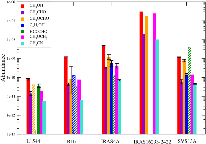
Figure 1: The evolution of abundances in different stages of low-mass star-forming regions is shown. The left panel shows the abundances obtained from the rotational diagram method (dashed parts are the upper limits), and the right panel depicts the same obtained with the MCMC fit. Black vertical lines represent the error bars. For CH₃OCH₃ in L1544 and B1b, the lines have the same upstate energy, so a rotation diagram cannot be performed, and the column density is calculated using simple LTE fitting. For CH₃OCH₃ in SVS13A, the column density is calculated using the value from Bianchi et al. (2019) scaling it for 30$\arcsec$ beam. A new class 0 source, IRAS16293-2422 (22 L_⊙), is included where CH₃OH, CH₃CHO, CH₃OCHO, CH₃OCH₃ and CH₃CN is observed (Cazaux et al., 2003).

3 Results & Discussions

The main goal of this work is to find the correlation between the observed COMs in various evolutionary phases of star-forming regions. Observing all the instances of a single low-mass star-forming region is impossible. Instead, it is beneficial to selectively follow some evolutionary stages of similar types of the ongoing process before the formation of stars to have an overview of the complete process. Though it is not expected that all the targeted regions would follow a similar footprint, it gives an overall idea of the general low-mass star-formation process. We were able to identify several transitions of interstellar COMs, i.e methanol (CH₃OH), acetaldehyde (CH₃CHO), methyl formate (CH₃OCHO), ethanol (C₂H₅OH), propynal (HCCCHO), dimethyl ether (CH₃OCH₃) and methyl cyanide (CH₃CN) in different sources.

We apply two robust LTE methods namely rotational diagram (RD) and Monte Carlo Markov Chain (MCMC) fitting, to derive the column density and excitation temperature of a species. The details description of RD analysis and MCMC method are discussed in the section C and D, respectively. The obtained column densities and temperature from rotational diagram analysis are summarized in Table 11. The rotation diagram plots are shown in 7, 8, 9, 10, 11, 12, 13 . The variable parameters and the ranges used for the MCMC method and the best-fitted values are summarized in Table 1. In addition, Table 2 compares the abundances obtained through MCMC fitting and rotational diagram analysis with earlier findings. It depicts that our results are consistent with the earlier results. The values obtained using both methods differ from the previously obtained values within a factor of 0.17-5.02. Also, the abundances obtained from rotational diagram analysis and MCMC fitting are almost similar and differ within a minimal range, which justifies the accuracy of the results obtained from the two methods. In the left panel of Figure 1, we show how the abundances obtained from the rotational diagram method varies in different sources, whereas the right panel shows similar results obtained with the MCMC fitting method. The results obtained from our analysis are discussed here with individual species. The column density values of H₂ in different sources are used from literature to calculate the abundances. The values are noted in Table 11 and in section 2.3.

3.1 Observed species

3.1.1 CH₃OH

Since methanol is a major chemical constituent of the various phases of star formation, its analysis has become of utmost importance. Previously, Vastel et al. (2014) identified CH₃OH emission in L1544 from the ASAI data and obtained a column density $3\times 10^{13}$ cm^-2 using non-LTE approximation. They concluded that methanol lines are likely originated from $\sim$ 8000 au, where the temperature is $\sim$ 10 K. Methanol was previously detected in B1-b using IRAM 30m telescope by Öberg et al. (2009) with a column density of $2.5\times 10^{14}$ cm^-2. In IRAS4A, Maret et al. (2005) obtained a column density $5.1\times 10^{14}$ cm^-2. Here, we have identified several transitions of CH₃OH in all four sample sources (see Table 6). The obtained values of column densities and excitation temperatures are noted from rotational diagram are prsented in Table 11 and same for MCMC fitting, it is noted in Table 1. We have performed MCMC fitting considering a single component of the detected CH₃OH transitions in L1544, B1-b, and SVS13A, and we get a good fit. In the case of class 0 protostar IRAS4A, we found that a two-component fit is required for the rotational diagram of methanol: (1) having E_up $>$ 50 K (hot component), (2) having E_up $<$ 50 K (cold component). Similarly in the MCMC method, we obtain a good fit when we are considering two components. The chemical evolution of CH₃OH with respect to the evolutionary stages of the star formation is represented by red bars in the left (RD) and right (MCMC) panels of Fig. 1. It shows that the methanol abundance gradually increases from a minimum value in L1544 to a maximum value in IRAS16293-2422. The increase in abundance might be attributed due to the gradual rise in temperature. Since a lower temperature (10-20 K) is efficient for the ice phase hydrogenation reactions, methanol formation by successive hydrogen additions to CO could be possible during the prestellar core phase.

$$\rm{CO\rightarrow HCO\rightarrow H_{2}CO\rightarrow CH_{2}OH/CH_{3}O\rightarrow CH_{3}OH}$$

However, at this stage, the thermal desorption is not efficient enough (Das et al., 2018, having a binding energy of 5264 K) to transfer the ice phase methanol contents to the gas phase. The non-thermal desorptions (Öberg et al., 2009; Garrod et al., 2007) are mainly responsible for the observed gas-phase abundance of methanol at this stage. Furthermore, the cloud evolves into a first hydrostatic core and then a protostar phase. In the protostar phase, methanol would also be formed by radical-radical surface reaction, $\rm{CH_{3}+OH\rightarrow CH_{3}OH}$. As a result, temperature increases, eventually enhancing the chance of production and their release by thermal desorption. We get a less abundance of methanol in SVS13A (class I object). A decrease in the abundance of methanol for the class I object may occur due to the lower methanol formation rate in the class I phase than in the class 0 phase because of the competition between the reaction and thermal desorption of the reactants.

Scibelli & Shirley (2020) surveyed the presence of complex organic molecules in starless and prestellar cores within the Taurus Molecular Cloud by ARO 12m telescope on Kitt Peak (beam size $\sim 62.3^{{}^{\prime\prime}}$). They obtained a methanol abundance $(0.53-3.36)\times 10^{-9}$, and excitation temperature ranging from $6.79-8.66$ K for all 31 cores. From the rotational diagram analysis, we obtained a comparatively lower abundance of methanol $\sim 8.02\times 10^{-11}$, in L1544 and an excitation temperature of $8.6$ K. Scibelli & Shirley (2020) found that the less evolved regions have comparatively higher methanol abundance than more evolved regions. Since the L1544 is more evolved than the sources studied by Scibelli & Shirley (2020), a comparatively lower abundance of methanol is consistent with the observed trend.

3.1.2 CH₃CHO

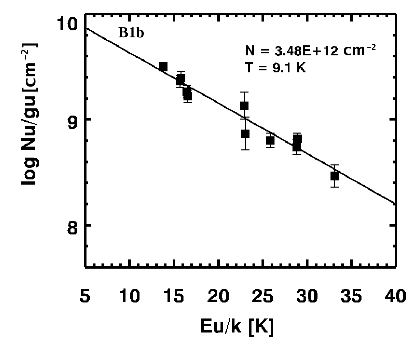
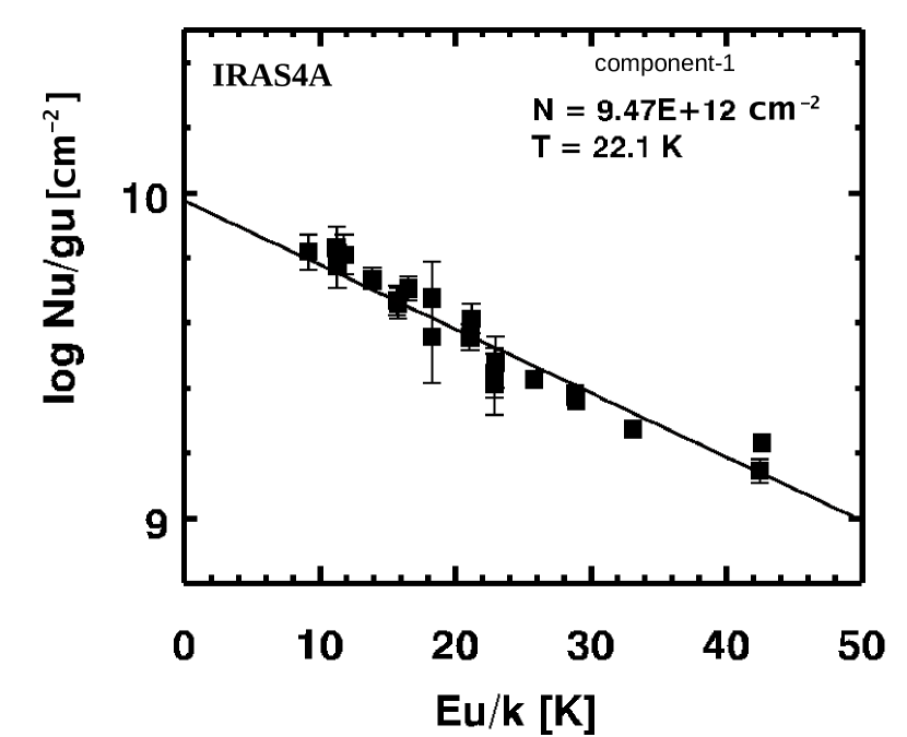
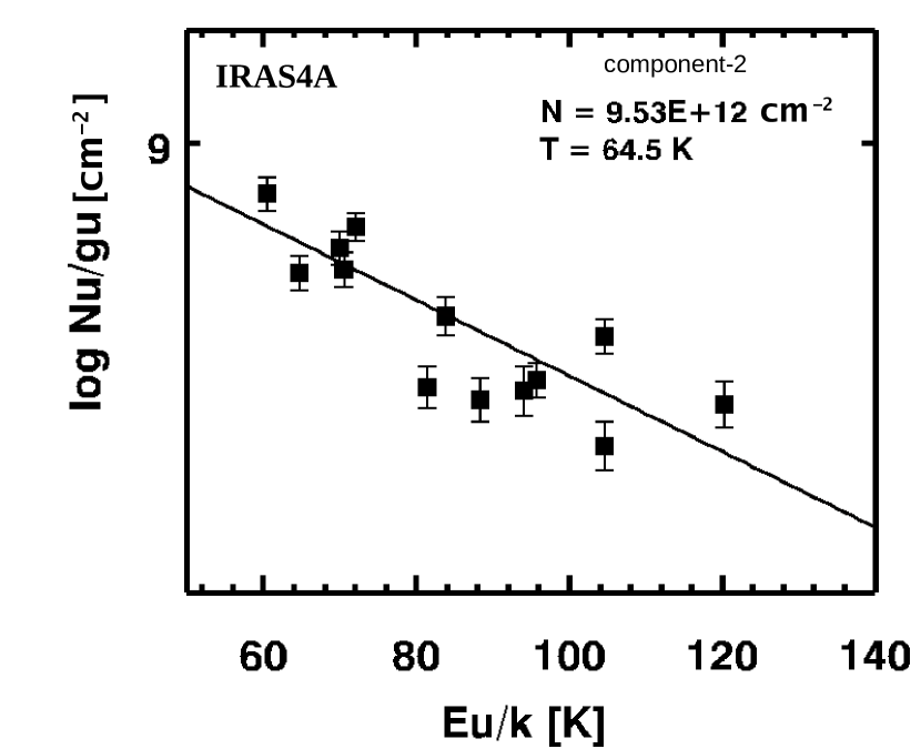
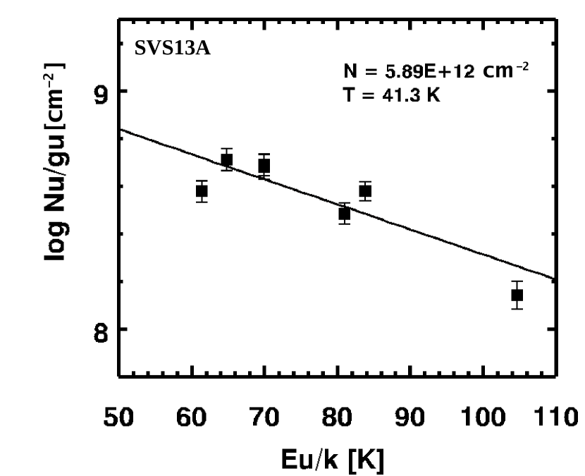
Figure 8: Rotational diagram for CH₃CHO obtained for various sources. The symbols represent the same as those depicted in Figure 7.

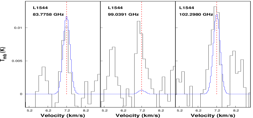
Figure 8: Same as Figure 1 for $\rm{HCCCHO}$.

Acetaldehyde, is an asymmetric top molecule with a widespread presence in the various evolutionary phases of star formation. We have identified multiple transitions of CH₃CHO in all the selected sources. Fitted line parameters of this species are summarised in Table 7. The upper state energy of the observed lines ranges from $9$ to $121$ K. Jiménez-Serra et al. (2016) obtained a column density 1.2 $\times$ 10¹² cm^-2 towards the dense, highly extinguished continuum peak within the inner 2700 au and $3.2\times 10^{12}$ cm^-2 towards a low-density shell located at 4000 au from the core center. However, we obtain a very similar column density of $1.25\times 10^{12}$ cm^-2 for acetaldehyde in our work. In B1-b, a column density of $1.5\times 10^{12}$ cm^-2 was obtained by Cernicharo et al. (2012) with the MADEX code assuming the excitation temperature of 10 K. From our rotation diagram analysis, we found the column density $3.5\times 10^{12}$ cm^-2 of this species. Holdship et al. (2019) and Bianchi et al. (2019) observed CH₃CHO towards IRAS4A and SVS13A and obtained a column density of $2.6\times 10^{12}$ cm^-2 and $1.2\times 10^{16}$ cm^-2, respectively using single-dish telescope. From our rotation diagram analysis, we yield the column densities of $9.5\times 10^{12}$ cm^-2 and $5.9\times 10^{12}$ cm^-2 for IRAS4A and SVS13A, respectively. Similar to the CH₃OH, for CH₃CHO, two components are observed in the rotational diagram analysis (see Figure 8) in IRAS4A, (1) E_up $>$ 50 K (hot component) and (2) cold component having E_up $<$ 50 K. We obtain a temperature of $22.1$ K for the low excitation lines and $64.5$ K for the high excitation lines from RD analysis. Similarly, a two-component MCMC fit is performed and yields a temperature of $71.2$K and $11.1$ K for components 1 and 2, respectively. It is noticed that the results derived from the two methods are very similar. The violet-colored bar lines in Figure 1 represent the variation of its abundance and it shows the same behavior as $\rm{CH_{3}OH}$ throughout the evolutionary stages of star formation. Scibelli & Shirley (2020) obtained acetaldehyde abundance $(0.6-3.9)\times 10^{-10}$, and excitation temperature 3.57 K. From the rotational diagram analysis, we obtained a comparatively lower abundance of acetaldehyde $\sim 1.4\times 10^{-11}$ in L1544 and an excitation temperature of 6 K. Similar to CH₃OH since the L1544 is more evolved than the sources studied by Scibelli & Shirley (2020), a comparatively lower abundance of acetaldehyde is consistent with the observed trend.

3.1.3 CH₃OCHO

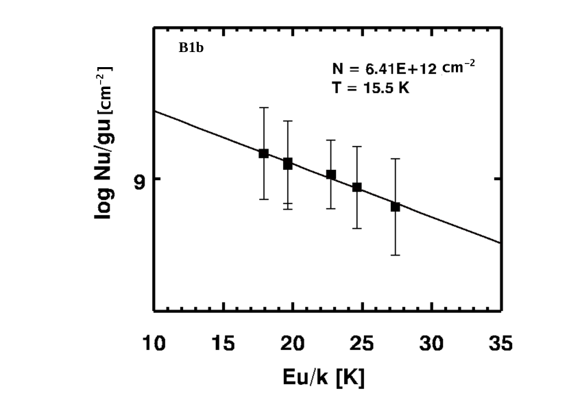
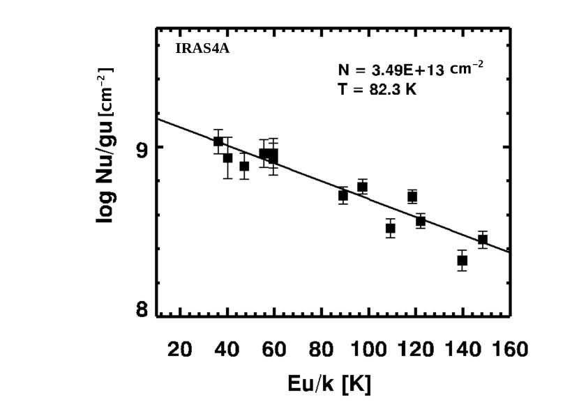
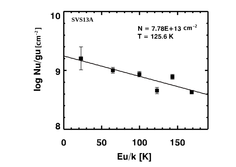
Figure 9: Rotational diagram for CH₃OCHO obtained for various sources. The symbols represent the same as those depicted in Figure 7.

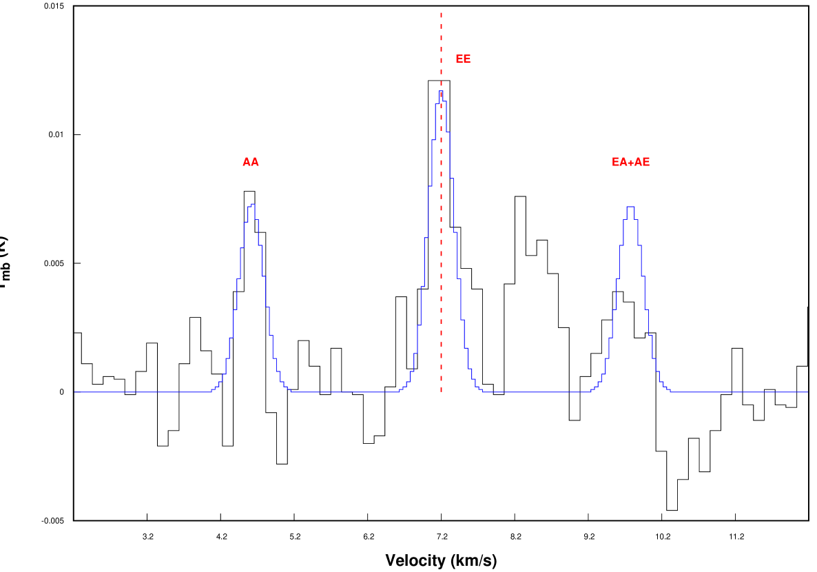
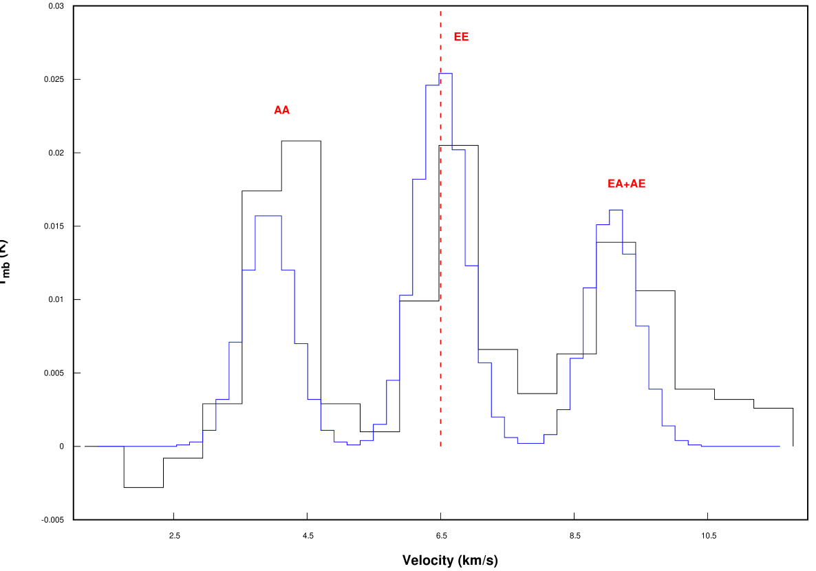
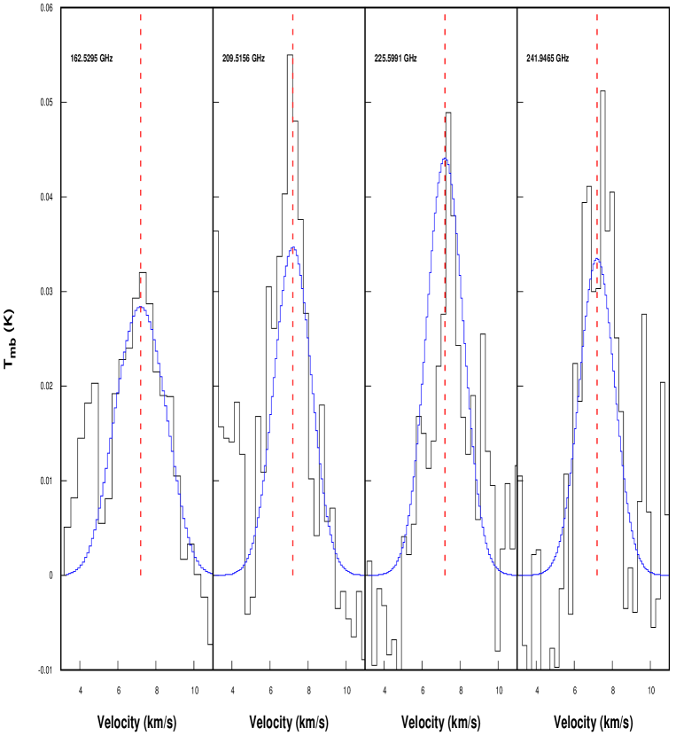
Figure 9: Same as Figure 1 for $\rm{CH_{3}OCH_{3}}$ in L1544 (left), B1-b (right) and IRAS4A (bottom).

Methyl formate is a simple asymmetric top complex organic species observed in most star-forming regions. Its isomers, acetic acid (CH₃COOH) and glycolaldehyde (HCOCH₂OH), are comparatively less abundant. Observing complex molecules in a prestellar core is always challenging because of their low temperature. Jiménez-Serra et al. (2016) identified methyl formate in L1544 with IRAM 30 m at two positions; one at the center of the core and another at the same place where the peak abundance of methanol arises. They found a column density of $(4.4\pm 4.0)\times 10^{12}$ cm^-2 and $(2.3\pm 1.4)\times 10^{12}$ cm^-2 at these two position respectively. Cernicharo et al. (2012) observed this species towards B1-b, and derived a total column density of $3\times 10^{12}$ cm^-2. Bottinelli et al. (2004) observed CH₃OCHO towards the low-mass protostar IRAS4A and derived a column densities of $5.5\times 10^{16}$ cm^-2 and $5.8\times 10^{16}$ cm^-2 for A-CH₃OCHO and E-CH₃OCHO, respectively. Bianchi et al. (2019) identified CH₃OCHO transitions towards SVS13A, and obtained a column density of $1.3\times 10^{17}$ cm^-2. In the prestellar core L1544, one transition at 90.22765 GHz is tentatively detected. An upper limit of column density $3.7\times 10^{12}$ cm^-2 is estimated using LTE method (see Table 10). For B1-b, IRAS4A, and SVS13A, many transitions are detected, and the results from RD analysis and MCMC method are shown in Table 11 and 1, respectively. The RD plot for CH₃OCHO is shown in Figure 9 and the MCMC fitting is shown in Figure 6.
We have found that $\rm{CH_{3}OCHO}$ follow a similar pattern as methanol and acetaldehyde in its evolution from the prestellar core phase to the class I stage, as represented by an orange-colored bar line in Figure 1. Unlike methanol and acetaldehyde, no ice phase hydrogenation reactions are directly involved in forming $\rm{CH_{3}OCHO}$. Instead, it is the radical-radical reaction between $\rm{CH_{3}O}$ and HCO that can form ice phase $\rm{CH_{3}OCHO}$:

$${\rm CH_{3}O+HCO\rightarrow CH_{3}OCHO}.$$

The activities are restricted at low temperatures due to the high binding energy of these radicals i.e., 4400 K for CH₃O (Wakelam et al., 2017) and 2206 K for HCO (Das et al., 2018). However, it plays an active role in the warmer region. Moreover, the binding energy of $\rm{CH_{3}OCHO}$ (6295 K, https://kida.astrochem-tools.org) is comparatively higher than the methanol and acetaldehyde (Das et al., 2018, 5264 and 4573, respectively). The decline in the CH₃OCHO abundance at the class I stage would be attributed to the favorable sublimation rate over the reaction rate of radicals and its subsequent gas phase destruction after desorption.

3.1.4 $\rm{C_{2}H_{5}OH}$

Ethanol (C₂H₅OH) emission was detected for the first time in 1975 toward Sagittarius B2. It was observed with the help of one of the pioneering radio telescopes of the twentieth century, the 11 m radio telescope of the National Radio Astronomy Observatory (NRAO, Zuckerman et al. (1975)). It has been observed towards low and high mass in both the star-forming regions. Due to the orientation of the OH group, ethanol consists of two different conformers, one is anti, and another one is gauche. A gauche⁺ and gauche ^- state forms when the tunnelling between the two equivalent gauche conformers lifts the degeneracy. Recently, Bianchi et al. (2019) performed ab initio quantum chemical calculations to characterize the geometry and energy of ethanol conformers with high accuracy. In this work, no clear C₂H₅OH lines are detected in L1544. In IRAS4A and SVS13A, multiple transitions of ethanol are clearly identified. Three possible transitions of C₂H₅OH are detected toward B1-b. However, the transition at 135.989923 GHz is below 3$\sigma$, and the other transition at 270.444085 GHz is blended. Only one unblended transition at 131.502781 GHz is detected. Therefore, we consider ethanol is tentatively detected in this source and derived upper limit of column density $\sim 1.0\times 10^{13}$ cm^-2 ( see Table 10). Figure 1 shows that the abundance is maximum in IRAS4A (class 0). It would form on grain surface by radical-radical reaction between $\rm{C_{2}H_{5}}$ and OH. Das et al. (2018) estimated binding energy of $\rm{C_{2}H_{5}}$ and OH to be 2081 K and 3781 K, respectively. The absence of $\rm{C_{2}H_{5}OH}$ in the prestellar core may be due to the mobility of these two radicals being limited at low temperatures. Also, the binding energy of ethanol itself is high (Wakelam et al., 2017, 5400 K) to release in the gas phase. A comparatively reduced abundance of $\rm{C_{2}H_{5}OH}$ in the class I stage would be due to the lack of production of it by the radical-radical reaction at such a high temperature and its subsequent destruction after its desorption.

3.1.5 $\rm{HCCCHO}$

Propynal ($\rm{HCCCHO}$) was discovered in a cold cloud, TMC-1, using the NRAO’s 42.7 m radio telescope at Green Bank (Irvine et al., 1988). The first laboratory-based infrared spectra of amorphous and crystalline forms of propynal were presented by Hudson & Gerakines (2019) at multiple temperatures. Due to its band’s intensity and spectral position, it becomes an attractive candidate for an astronomical search involving interstellar ices. Here, we identify only three transitions of HCCCHO in L1544. With the IRAM 30 m telescope, Jiménez-Serra et al. (2016) carried out high-sensitivity single-pointing 3 mm observations toward the dust-continuum peak in L1544. They detected a single transition for HCCCHO at 83.775842 GHz. We also identify the same transition (9_0,9 - 8_0,8) along with another two transitions. Our RD analysis yields a column density of $3.2\times 10^{12}$ cm^-2 in L1544. We are not able to identify any clear transitions in other sources. However, we estimate an upper limit of HCCCHO for these sources (see Table 10). Loison et al. (2016) reported a single line at 83.775832 GHz (9_0,9 - 8_0,8) of propynal in B1-b, having the column density of 7.9 $\times$ 10¹¹ cm^-2 but we and Margulès et al. (2020) did not observe this particular transition from the ASAI data. Margulès et al. (2020) estimated an upper limit of HCCCHO based on 102.298 GHz transition, but in our observation, we have seen that this transition is shifted and is also blended with s-Propanal. Although the line at 93.043 GHz is slightly shifted from the peak but it is not blended with any other lines. Therefore, On the basis of this transition, we made an upper limit of column density ($\sim$ 2.56 $\times$ 10¹² cm^-2) in B1-b.

The variation of abundance of HCCCHO in various phases of star formation is shown in Figure 1 with a green colored bar. We notice that the abundance is relatively low in L1544. It remains roughly the same in B1-b. In the case of IRAS4A, it increases a little. On the other hand, we get a high abundance in SVS13A.

Given that the majority of the abundances provided here are based on the predicted upper limit of propynal, making a strong statement regarding the evolution related to propynal would not be justified. However, in the ice phase, the formation of HCCCHO can process by the following reactions:

$${\rm O+CH_{2}CCH\rightarrow HCCCHO+H}$$

$${\rm C_{2}H+H_{2}CO\rightarrow HCCCHO+H}$$

The binding energy value of the reactants obtained from Das et al. (2018) are 770 K, 3238 K, 3315 K, and 3851 K for O, $\rm{CH_{2}CCH}$, C₂H, and H₂CO, respectively. So at the low temperature, HCCCHO formation could process by oxygen addition, whereas in the warmer region, by C₂H and H₂CO. The highest column density obtained at SVS13A indicates that warm chemistry would be efficient.

3.1.6 $\rm{CH_{3}OCH_{3}}$

Dimethyl ether (DME) is an asymmetric top molecule with two CH₃ groups, which undergoes a large amplitude motion along CO-bond. The two internal rotations cause the splitting of a rotational level into four sub-states AA, EE, AE, and EA. DME was detected in the Orion nebula by Snyder et al. 1974. A gas phase formation route for DME was proposed by Blake et al. 1987. Its presence in the high-mass star-forming regions (Turner et al., 1999; Sutton et al., 1995; Nummelin et al., 2000) and low-mass binary system (Cazaux et al., 2003; Kuan et al., 2004) have been observed. From the experiments, observations, and theoretical perspectives, Peeters et al. (2006) discussed the fate of DME in various astrophysical environments. We have identified only one transition (3_1,3 - 2_0,2) of DME with four sub-states AA, AE, EA, and EE in L1544. The EE and AA sub-states are clearly resolved in our study, whereas the EA and AE are overlapped with each other. It is not possible to perform RD analysis as those sub-states have the same upper-state energy. We estimate a column density of $1.6\times 10^{12}$ cm^-2 from LTE fitting. Jiménez-Serra et al. (2016) also observed the same transition in their work and mentioned a column density of $1.5\times 10^{12}$ cm^-2. In B1-b, we have identified four similar sub-states identical to those observed in L1544. We derive a column density of $6.0\times 10^{12}$ cm^-2 in B1-b from LTE fitting. In IRAS4A, we have observed four unblended transitions, and each of them consists of four sub-states, but they are overlapped with each other. The integrated intensity is obtained with Gaussian fitting and then divided according to their $S\mu^{2}$ values (Shimonishi et al., 2016). The transitions with maximum intensity among these sub-states are considered for the rotation diagram analysis to calculate the rotation temperature and column density. Only these transitions are noted in Table 8. We get a rotational temperature of $61.1$ K and column density of $1.2\times 10^{13}$ cm^-2 for this species in this source. The observed transitions of DME in SVS13A have asymmetric line profiles (transitions are not mentioned here; see Bianchi et al. 2019), and hence Gaussian fit is not possible to perform for these types of transitions. Bianchi et al. (2019) have calculated the column density of DME for asymmetric line profile (see method described in Appendix A1 in Bianchi et al. 2019). They used a source size of $0.3\arcsec$ to derive the column density ($1.4\times 10^{17}$ cm^-2) of this species. We use their value after scaling by beam filling factor considering the source size $30\arcsec$ and the obtained value is $\sim 1.4\times 10^{13}$ cm^-2. We also perform LTE fitting and get a good fit with a column density a few times higher than the scaled value. We use the above-mentioned scaled value in this work.

The variation of the abundance of DME in different sources which are in different phases of star-formation is shown in Figure 1 using a magenta-colored bar. We also observed a rising tendency from the L1544 to the IRAS4A and IRAS16293-2422 for DME, similar to what was shown with methanol, acetaldehyde, and methyl formate. Whereas its value gets decreased in SVS13A.

DME is considered to be formed either in the grain surface (Cuppen et al., 2017) or gas phase (Balucani et al., 2015). Both the hydrogenation and radical-radical pathways were involved in the ice phase formation of DME:

$${\rm CH_{3}CHO+H\rightarrow CH_{3}OCH_{2}},$$

$${\rm CH_{3}OCH_{2}+H\rightarrow CH_{3}OCH_{3}},$$

$${\rm CH_{3}+CH_{3}O\rightarrow CH_{3}OCH_{3}}.$$

Both the hydrogenation and the radical-radical route form dimethyl ether. Like methanol, acetaldehyde, and methyl formate, its abundance gradually increases throughout the evolutionary phase up to the class 0 phase and then decreases in the class I phase.

3.2 $\rm{CH_{3}CN}$

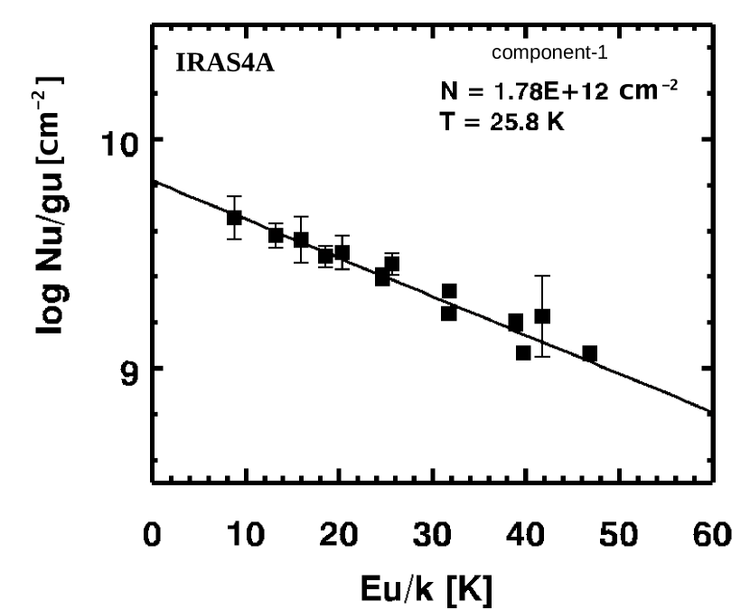
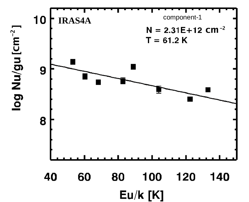
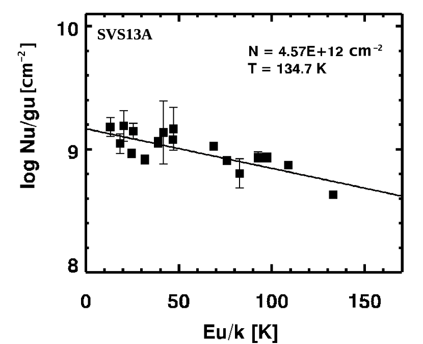
Figure 13: Rotational diagram for CH₃CN obtained for various sources. The symbols represent the same as those depicted in Figure 7.

Methyl cyanide or CH₃CN is a symmetric-top molecule with a high dipole moment of $\sim$ 3.91 debyes. The K-ladders in the rotational level of CH₃CN can be excited only by collisional excitation. Hence CH₃CN can be a very good tracer to calculate the kinetic temperature of the molecular clouds. We have detected several transitions of CH₃CN in all the selected sources. Similar to the CH₃OH and CH₃CHO, for CH₃CN, a two components fit is required for the rotational diagram of methyl cyanide (see Figure. 13) in IRAS4A, (1) E_up $>$ 50 K (hot component) and (2) E_up $<$ 50 K (cold component). RD analysis yields a temperature of 61.2 K for the high excitation lines and 25.8 K for the low excitation lines. Similarly, a two-component MCMC fit is performed and yields a temperature of 70.1K and 21.0 K for hot component and cold component, respectively.
Taking the ratio between two transitions of the same frequency band can nullify various uncertainties obtained from observation. Here we used the line ratios of different CH₃CN transitions observed to calculate the kinetic temperature. Different K_a ladders are connected by collisional excitation. The relative population of two K_a ladders follows the Boltzmann equation at kinetic temperature. Considering the selection rules mentioned in Mangum & Wootten (1993), we calculated the line ratio between two transitions. Details of the selection rule and the method are described in Das et al. (2019); Mondal et al. (2023). Some selected line ratios are calculated ($\frac{J1_{k_{a}}-J2_{k_{a}}}{J3_{k_{a^{\prime}}}-J4_{k_{a^{\prime}}}}$). Using LTE approximation, the ratio (R) between two transitions satisfying the conditions mentioned in Mangum & Wootten (1993) is, R = S_R exp(D/T_K), where $D=E(J3,k_{a^{\prime}})-E(J1,k_{a})$ and $S_{R}=\frac{S_{J1k_{a}}}{S_{J3k_{a^{\prime}}}}$.

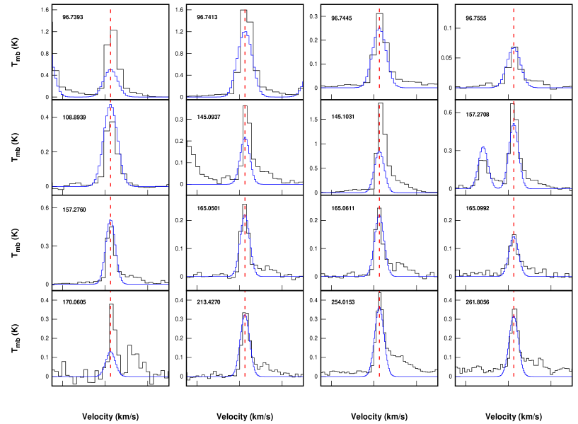
Figure 2: Same as Figure 1 for $\rm{CH_{3}OH}$ in B1-b.

Under the LTE approximation, as the kinetic temperature is considered equal to the excitation temperature, we calculated the kinetic temperatures for different CH₃CN k-ladder transitions for the sources (L1544, Barnard1 b, IRAS4A, SVS13A) using the above-mentioned formula. Calculated values of kinetic temperatures for all the CH₃CN transitions are mentioned in Table 4. In Figure 2, we plotted the average kinetic temperature obtained from this calculations for the transitions having E${}_{up}>50$ K with the solid blue line, and the dashed blue line in Figure 2 is the same for transitions having E${}_{up}<50$ K.

Table 3: Calculation of kinetic temperature using line ratio of observed CH₃CN transitions.

Source	Frequency	Quantum No.	Eup	$\int$Tmbdv	Sij	R	Tk	Average Tk
	(GHz)		(K)	(K.km.s-1)			(K)	(K)
L1544	91.985314	$5_{1}$ - $4_{1}$	20.4	0.05	6.61439	$\frac{5_{0}-4_{0}}{5_{1}-4_{1}}$	5.12	5.12
	91.987087	$5_{0}$ - $4_{0}$	13.2	0.068	2.2051
B1-b	91.985314	$5_{1}$ - $4_{1}$	20.4	0.034	6.61439	$\frac{5_{0}-4_{0}}{5_{1}-4_{1}}$	4.41	4.41
	91.987087	$5_{0}$ - $4_{0}$	13.2	0.058	2.2051
IRAS4A	128.75703	$7_{3}$ – $6_{3}$	89	0.089	15.74921	$\frac{7_{2}-6_{2}}{7_{3}-6_{3}}$	33.79
	128.769436	$7_{2}$ - $6_{2}$	53.3	0.144	8.85861
	128.769436	$7_{2}$ - $6_{2}$	53.3	0.144	8.85861	$\frac{7_{1}-6_{1}}{7_{2}-6_{2}}$	46.24
	128.776881	$7_{1}$ – $6_{1}$	31.9	0.244	9.44898
	128.75703	$7_{3}$ – $6_{3}$	89	0.089	15.74921	$\frac{7_{1}-6_{1}}{7_{3}-6_{3}}$	37.58
	128.776881	$7_{1}$ – $6_{1}$	31.9	0.244	9.44898
	128.75703	$7_{3}$ – $6_{3}$	89	0.089	15.74921	$\frac{7_{0}-6_{0}}{7_{3}-6_{3}}$	23.19
	128.779363	$7_{0}$ - $6_{0}$	24.7	0.285	3.1501
	128.769436	$7_{2}$ - $6_{2}$	53.3	0.144	8.85861	$\frac{7_{0}-6_{0}}{7_{2}-6_{2}}$	16.66
	128.779363	$7_{0}$ - $6_{0}$	24.7	0.285	3.1501
	147.163244	$8_{2}$ – $7_{2}$	60.4	0.098	10.33654	$\frac{8_{1}-7_{1}}{8_{2}-7_{2}}$	26.44	48.60	E${}_{up}>$ 50 K
	147.171751	$8_{1}$ – $7_{1}$	38.9	0.232	10.85164
	147.163244	$8_{2}$ – $7_{2}$	60.4	0.098	10.33654	$\frac{8_{0}-7_{0}}{8_{2}-7_{2}}$	14.17
	147.174588	$8_{0}$ – $7_{0}$	31.8	0.258	3.61771
	165.540377	$9_{3}$ – $8_{3}$	104	0.131	22.05132	$\frac{9_{2}-8_{2}}{9_{3}-8_{3}}$	106.31
	165.556321	$9_{2}$ - $8_{2}$	68.3	0.098	11.7908
	165.556321	$9_{2}$ - $8_{2}$	68.3	0.098	11.7908	$\frac{9_{1}-8_{1}}{9_{2}-8_{2}}$	28.45
	165.565891	$9_{1}$ – $8_{1}$	46.9	0.216	12.25078
	165.540377	$9_{3}$ – $8_{3}$	104	0.131	22.05132	$\frac{9_{1}-8_{1}}{9_{3}-8_{3}}$	52.49
	165.565891	$9_{1}$ – $8_{1}$	46.9	0.216	12.25078
	165.540377	$9_{3}$ – $8_{3}$	104	0.131	22.05132	$\frac{9_{0}-8_{0}}{9_{3}-8_{3}}$	29.16
	165.569081	$9_{0}$ – $8_{0}$	39.7	0.22	4.08322
	165.556321	$9_{2}$ - $8_{2}$	68.3	0.098	11.7908	$\frac{9_{0}-8_{0}}{9_{2}-8_{2}}$	15.30
	165.569081	$9_{0}$ – $8_{0}$	39.7	0.22	4.08322
	73.588799	$4_{1}$ – $3_{1}$	16	0.127	5.16717	$\frac{4_{0}-3_{0}}{4_{1}-3_{1}}$	5.20
	73.590218	$4_{0}$ – $3_{0}$	8.8	0.169	1.72263
	91.979994	$5_{2}$ – $4_{2}$	41.8	0.082	5.78723	$\frac{5_{1}-4_{1}}{5_{2}-4_{2}}$	33.07
	91.985314	$5_{1}$ – $4_{1}$	20.4	0.179	6.61439
	91.985314	$5_{1}$ – $4_{1}$	20.4	0.179	6.61439	$\frac{5_{0}-4_{0}}{5_{1}-4_{1}}$	5.50
	91.987087	$5_{0}$ – $4_{0}$	13.2	0.221	2.2051
	91.979994	$5_{2}$ – $4_{2}$	41.8	0.082	5.78723	$\frac{5_{0}-4_{0}}{5_{2}-4_{2}}$	14.62
	91.987087	$5_{0}$ – $4_{0}$	13.2	0.221	2.2051
	110.381372	$6_{1}$ – $5_{1}$	25.7	0.233	8.03828	$\frac{6_{0}-5_{0}}{6_{1}-5_{1}}$	5.99	10.31	E${}_{up}<$ 50 K
	110.383499	$6_{0}$ – $5_{0}$	18.5	0.258	2.6798
	128.776881	$7_{1}$ – $6_{1}$	31.9	0.244	9.44898	$\frac{7_{0}-6_{0}}{7_{1}-6_{1}}$	5.74
	128.779363	$7_{0}$ - $6_{0}$	24.7	0.285	3.1501
	147.171751	$8_{1}$ – $7_{1}$	38.9	0.232	10.85164	$\frac{8_{0}-7_{0}}{8_{1}-7_{1}}$	5.89
	147.174588	$8_{0}$ – $7_{0}$	31.8	0.258	3.61771
	165.565891	$9_{1}$ – $8_{1}$	46.9	0.216	12.25078	$\frac{9_{0}-8_{0}}{9_{1}-8_{1}}$	6.45
	165.569081	$9_{0}$ – $8_{0}$	39.7	0.22	4.08322
SVS13A	110.364353	$6_{3}$ - $5_{3}$	82.8	0.08	12.40333	$\frac{6_{2}-5_{2}}{6_{3}-5_{3}}$	42.87
	110.374989	$6_{2}$ - $5_{2}$	47.1	0.109	7.34927
	110.364353	$6_{3}$ - $5_{3}$	82.8	0.08	12.40333	$\frac{6_{1}-5_{1}}{6_{3}-5_{3}}$	72.47
	110.381372	$6_{1}$ – $5_{1}$	25.7	0.114	8.03828
	110.364353	$6_{3}$ - $5_{3}$	82.8	0.08	12.40333	$\frac{6_{0}-5_{0}}{6_{3}-5_{3}}$	38.21
	110.383499	$6_{0}$ – $5_{0}$	18.5	0.093	2.6798
	220.709016	$12_{3}$ – $11_{3}$	133.2	0.265	31.00599	$\frac{12_{2}-11_{2}}{12_{3}-11_{3}}$	47.07
	220.73026	$12_{2}$ - $11_{2}$	97.4	0.294	16.07897
	220.74301	$12_{1}$ - $11_{1}$	76	0.278	16.4203	$\frac{12_{0}-11_{0}}{12_{1}-11_{1}}$	24.76	63.90	E${}_{up}>$ 50 K
	220.747261	$12_{0}$ - $11_{0}$	68.9	0.373	16.53946
	220.709016	$12_{3}$ – $11_{3}$	133.2	0.265	31.00599	$\frac{12_{1}-11_{1}}{12_{3}-11_{3}}$	83.68
	220.74301	$12_{1}$ - $11_{1}$	76	0.278	16.4203
	220.709016	$12_{3}$ – $11_{3}$	133.2	0.265	31.00599	$\frac{12_{0}-11_{0}}{12_{3}-11_{3}}$	66.27
	220.747261	$12_{0}$ - $11_{0}$	68.9	0.373	16.53946
	220.73026	$12_{2}$ - $11_{2}$	97.4	0.294	16.07897	$\frac{12_{0}-11_{0}}{12_{2}-11_{2}}$	135.87
	220.747261	$12_{0}$ - $11_{0}$	68.9	0.373	16.53946

Table 4: Calculation of kinetic temperature using line ratio of observed CH₃CN transitions.

Source	Frequency	Quantum No.	Eup	$\int$Tmbdv	Sij	R	Tk	Average Tk
	(GHz)		(K)	(K.km.s-1)			(K)	(K)
	91.979994	$5_{2}$ – $4_{2}$	41.8	0.067	5.78723	$\frac{5_{1}-4_{1}}{5_{2}-4_{2}}$	184.38
	91.985314	$5_{1}$ – $4_{1}$	20.4	0.086	6.61439
	91.985314	$5_{1}$ – $4_{1}$	20.4	0.086	6.61439	$\frac{5_{0}-4_{0}}{5_{1}-4_{1}}$	6.42
	91.987087	$5_{0}$ – $4_{0}$	13.2	0.088	2.2051
	91.979994	$5_{2}$ – $4_{2}$	41.8	0.067	5.78723	$\frac{5_{0}-4_{0}}{5_{2}-4_{2}}$	23.11
	91.987087	$5_{0}$ – $4_{0}$	13.2	0.088	2.2051			43.58	E${}_{up}<$ 50 K
	110.381372	$6_{1}$ – $5_{1}$	25.7	0.114	8.03828	$\frac{6_{0}-5_{0}}{6_{1}-5_{1}}$	8.04
	110.383499	$6_{0}$ – $5_{0}$	18.5	0.093	2.6798
	110.374989	$6_{2}$ - $5_{2}$	47.1	0.109	7.34927	$\frac{6_{0}-5_{0}}{6_{2}-5_{2}}$	33.64
	110.383499	$6_{0}$ – $5_{0}$	18.5	0.093	2.6798
	128.7768817	$7_{1}$ – $6_{1}$	31.9	0.092	9.44898	$\frac{7_{0}-6_{0}}{7_{1}-6_{1}}$	5.85
	128.779363	$7_{0}$ - $6_{0}$	24.7	0.105	3.1501

3.3 Abundance variation in different sources

We found a steadily increasing abundance from L1544 to IRAS4A and peaked at IRAS16293-2422 for CH₃OH, CH₃CHO, CH₃OCHO, C₂H₅OH, CH₃OCH₃ and CH₃CN and a reduced abundance in SVS13A. In contrast, the abundance of HCCCHO shows an increasing trend up to the SVS13A. The trend obtained with HCCCHO is based on the upper limit derived for most of the sources except L1544. In the case of C₂H₅OH, we could not even estimate an upper limit in L1544.

Scibelli & Shirley (2020) noticed that CH₃OH and CH₃CHO formed early and often in the starless prestellar stages and they proposed a chemical link between them at the early stages. However, this proposed linkage in the prestellar cores is yet to be observationally supported by the higher spatial resolution map. They pointed out the chemical linkage between CH₃OH and CH₃CHO by the gas phase reaction: $\rm{CH+CH_{3}OH\rightarrow CH_{3}CHO+H}$ This reaction was experimentally studied by Johnson et al. (2000), who found it to be barrierless. Vasyunin et al. (2017) considered this reaction for their chemical modeling of the prestellar core. However, in the UMIST database, this reaction is considered above 298 K only. In the KIDA database, this reaction yields, $\rm{CH+CH_{3}OH\rightarrow CH_{3}+H_{2}CO}$ in the 10-300 K range.

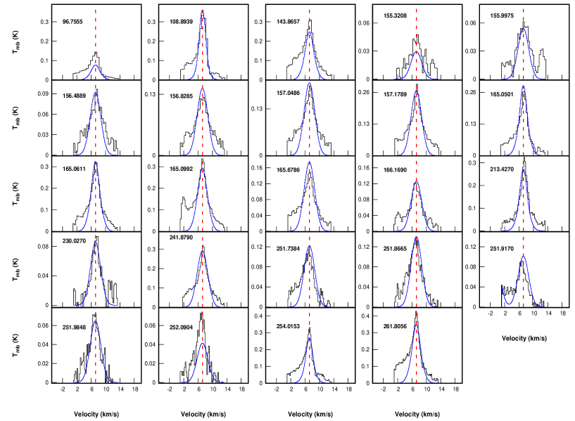
Figure 3: Same as Figure 1 for $\rm{CH_{3}OH}$ in IRAS4A.

The hydrogen column density in each source is required to derive the abundances of the species and look out for their linkage with the various evolutionary phases, if any. For the reliability of the abundance derivation from the obtained column density, we use the hydrogen column density obtained from a beam size comparable to the source size of the molecule (see Section 2.3). As our beam size varies from 30$\arcsec$ to 9$\arcsec$ in our frequency range, we could not resolve the molecular emission originating from the core. To have an idea, we plot the rotational temperature of two species and the kinetic temperature obtained from k-ladder calculation for CH₃CN (details in section 3.2) in all our sample sources. As usual, we found an increased temperature (see Figure 2) from L1544 to SVS13A. Moreover, we studied a particular transition of a species that is common in all the sources. Only one transition (96.755501 GHz) of CH₃OH is present in all the sources. We plot the integrated intensity of this transition of CH₃OH, and it is presented in Figure 3. It implies that the integrated intensity also shows a similar trend with the different sources at different stages as it was obtained for the abundances. Additionally, for acetaldehyde, we identified a transition at $211.2738$ GHz for all the sources except SVS13A. It shows an increasing trend. In IRAS4A and SVS13A, we identified a transition at $216.5819$ GHz and obtained a reduced integrated intensity in SVS13A compared to IRAS4A. Thus the adopted N(H₂) may not only be responsible for the obtained abundance trend.

Further, we check whether this transition is affected by any of the physical properties of the source. Hence, we plot the variation of FWHM of this transition (96.7555 GHz) for all the sources (see Figure 3). It depicts a steadily increasing trend from L1544 to SVS13A, and its value is comparable to the other observed transitions.

Since all these sources have different luminosity, in section 3.4, we discuss the linkage between the obtained abundances and source luminosity.

Except for the L1544, all our sample sources have multiple cores. The targeted position of all the sample sources in ASAI data is mentioned in Table 1. Our observed beam includes all the cores presented in each source, even with the highest frequency of our observation. So we need to check whether any chemical differentiation is present among the cores of each source and confirm that these cores follow the similar trend that we have obtained. Therefore, the high resolution interferometric data is required to verify the obtained trend for different sources in different stages. Since the analysis of the interferometric observation is out of scope for this paper, we discuss the interferometric observational results obtained by various authors in these sources in Section 3.4.1.

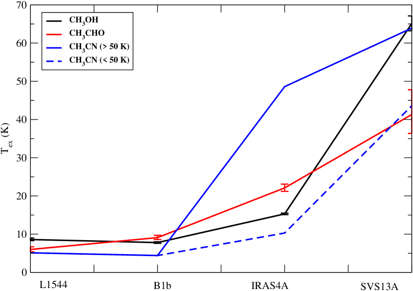
Figure 2: Excitation Temperature derived from rotation diagram for methanol (in black) and acetaldehyde (in red), respectively. Vertical lines represent the corresponding errors. Kinetic temperature calculated from Table 4 using CH₃CN transitions for high-temperature (solid blue) component and low-temperature (dashed blue) component present in IRAS4A and SVS13A.

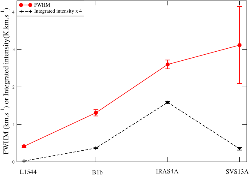
Figure 3: FWHM (red line) and integrated intensity (black-dashed) for 96.755501 GHz transition of methanol. The vertical lines represent the error bars.

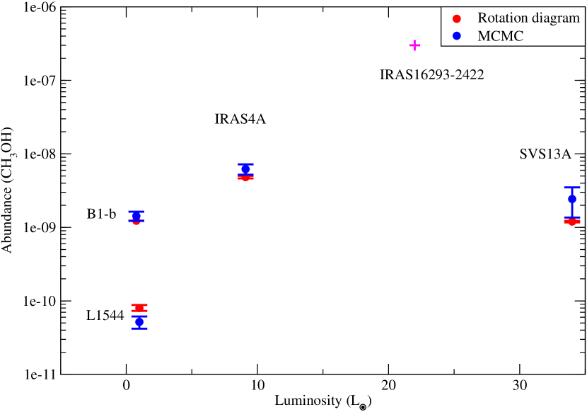
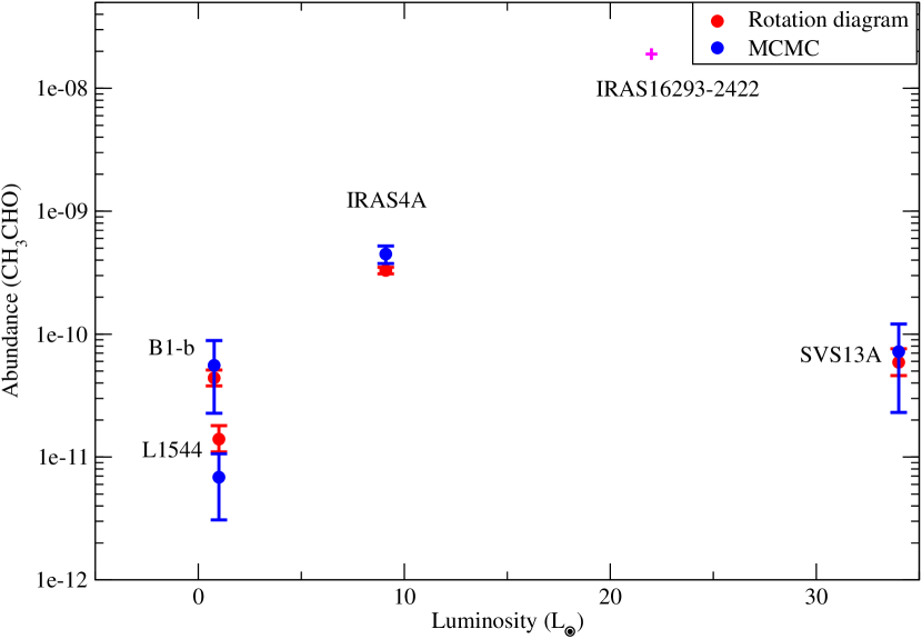
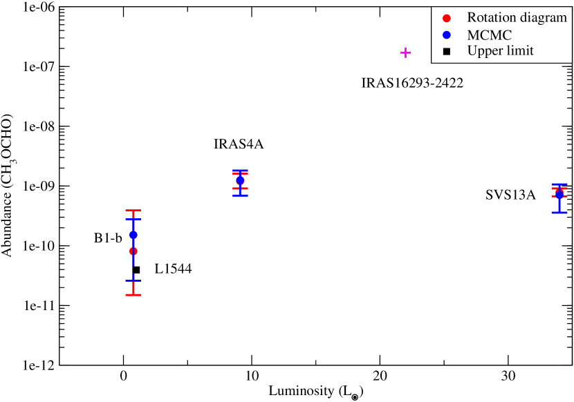
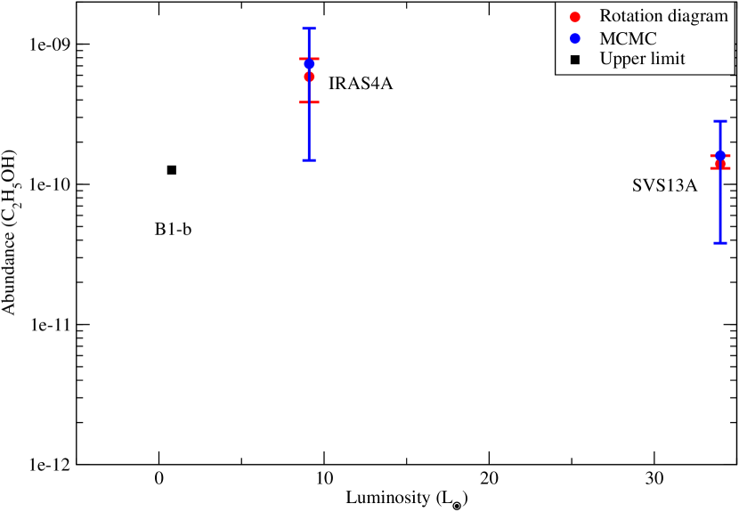
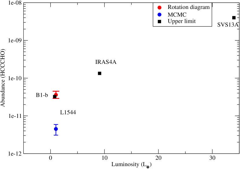
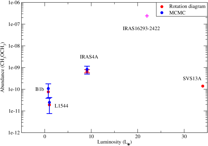
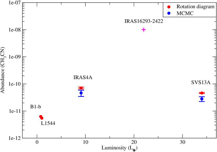
Figure 4: Abundance variation of CH₃OH, CH₃CHO, CH₃O-CHO, C₂H₅OH, HCCCHO, CH₃OCH₃ and CH₃CN shown with source luminosity. The red circle represents the value obtained from the rotational diagram, and the blue circle represents the same obtained from MCMC. The solid black squares represent the same calculated using upper limits. The plus sign (magenta) represents the abundance for IRAS4A 16293-2422 (22 L_⊙) taken from Cazaux et al. (2003). The vertical lines represent the error bars.

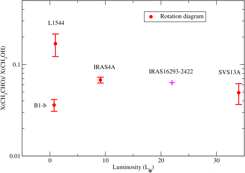
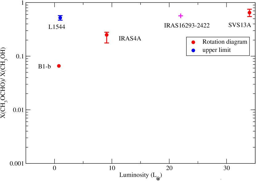
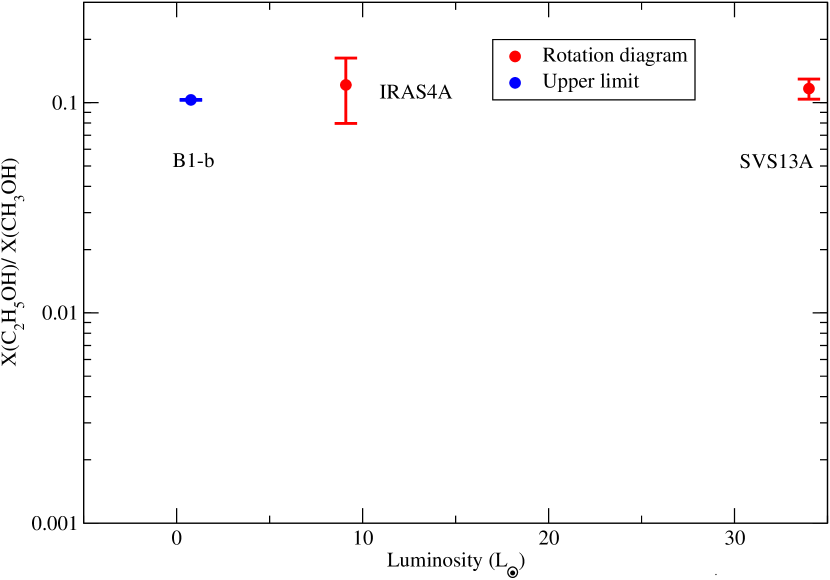
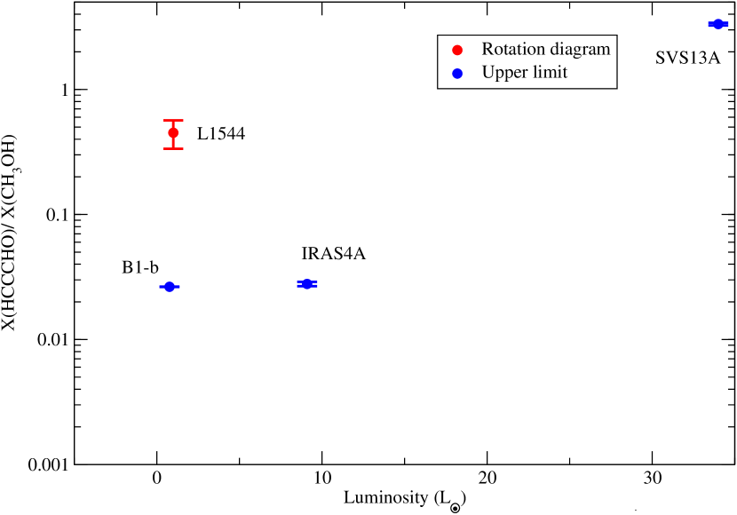
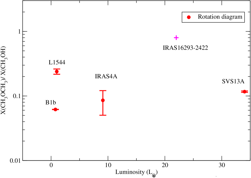
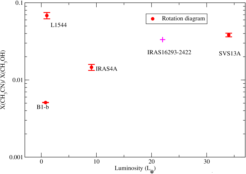
Figure 5: The abundance ratios of CH₃CHO, CH₃OCHO, C₂H₅OH, HCCCHO, CH₃OCH₃ and CH₃CN w.r.t methanol (CH₃OH) plotted with source luminosity. The red circles represent the value obtained from the rotational diagram, and the blue circles represent the same obtained from the upper limits. The plus sign (magenta) represents the abundance obtained for IRAS4A 16293-2422 (22 L_⊙) taken from Cazaux et al. (2003). Vertical lines represent the error bars.

3.4 Luminosity effect

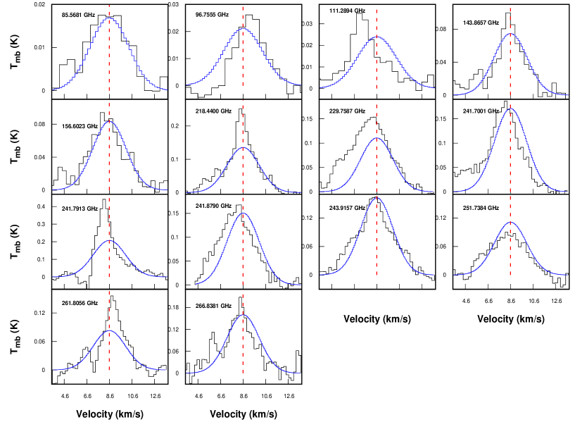
Figure 4: Same as Figure 1 for $\rm{CH_{3}OH}$ in SVS13A.

Source luminosity or bolometric luminosities may indicate the different evolutionary stages of star formation (Myers et al., 1998). The luminosity considered for L1544, B1-b, IRAS4A, and SVS13A are 1 L_⊙, 0.77 L_⊙, 9.1 L_⊙, and 34 L_⊙, respectively (Doty et al., 2005; Lefloch et al., 2018). Since the luminosity of SVS13A is much higher than the other sources considered here, we consider another object, IRAS16293-2422, lying between the IRAS4A and SVS13A to infer the trend related to the luminosity. IRAS16293-2422 is a solar-type Class 0 protostar in the eastern part of the $\rho$ Ophiuchi star-forming region at a distance of 120 pc. It has a bolometric luminosity of 22 L_⊙. We consider the obtained abundance of methanol, acetaldehyde, methyl formate, dimethyl ether and methyl cyanide for this source from Cazaux et al. (2003). The abundances of acetaldehyde, methyl formate, and dimethyl ether for this source were derived from the IRAM 30 m data, whereas methanol is from the JCMT. Figure 4 depicts the luminosity effect on the molecules considered in this study. The abundances obtained from rotational diagram analysis are shown with solid red circles, the MCMC method with solid blue circles, and the data obtained from (Cazaux et al., 2003, IRAS 16293-2422) with magenta crosses in Figure 4. The black solid squares are the values obtained by using the upper limit. It shows a similar behavior as discussed in Figure 1. In the case of IRAS 16293-2422, compared to another class 0 object, IRAS4A, a higher column density of these species was obtained by Cazaux et al. (2003). It may be due to a higher luminosity ($\sim 22$ L_⊙) for IRAS 16293-2422 compared to IRAS4A ($\sim$ 9.1 L_⊙).

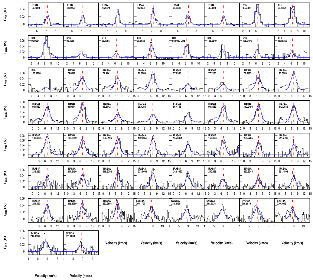
Figure 5: Same as Figure 1 for $\rm{CH_{3}CHO}$.

Since there are considerable uncertainties in deriving the abundances, it is beneficial to see the molecular ratio of some specific pairs to constrain our understanding better. Multi-line observations of methanol and several COMs toward the two low-mass protostars NGC 1333-IRAS2A and NGC 1333-IRAS4A with the PdBI at an angular resolution of 2 ${\arcsec}$ were carried out by Taquet et al. (2015). They calculated the ratio in column density of CH₃OCH₃ to C₂H₅OH in low mass protostar IRAS4A is about 0.7 considering the source size 0.5 $\arcsec$. In our case, we are getting this ratio with a similar value of 0.7 from the rotation diagram analysis values of IRAS4A. Figure 5 shows the abundance ratio with respect to methanol plotted with the luminosity of the sources. We did not find any specific trend by plotting the molecular ratio. But we found that methanol remains the most abundant among the species studied here (ratios are $<$1 except for HCCCHO). The first panel of Figure 5 displays the variation of the abundance ratio of acetaldehyde and methanol with luminosity. The ratio remains roughly invariant in IRAS4A, IRAS16293-2422 (class 0) and SVS13A (class I phase). The ratio between methyl formate and methanol in the second panel and between ethanol and methanol in the third panel of Figure 5 shows a similar nature.

3.4.1 Interferometric observations

It is well known that the evolution of COMs is linked with various evolutionary stages of star formation. We use the large program ASAI data to examine this aspect. We also include the previous interferometric observation to consolidate the obtained trend. Figure 6 shows the obtained abundance trend with the interferometric observation. In Table 5, we have noted the abundances and H₂ column density obtained with the interferometric observations.

There is considerable uncertainty in deriving the abundances of these molecules from the obtained column density. Marcelino et al. (2018b) presented the ALMA Band 6 spectral line observations at the angular resolution of $\sim 0.6$ $\arcsec$ towards B1-b. They extracted the spectra towards both protostars, B1b-S and B1b-N. However, it was found that B1b-S is rich in COMs, whereas B1b-N is free of COMs emission. They derived the column densities of ¹³CH₃OH for source sizes of 0.35 $\arcsec$. We utilize a value of ¹²C/¹³C = 60 in deriving the column density of ¹²CH₃OH from this. They also derived the column density of CH₃CHO, CH₃OCH₃, CH₃OCHO, and N(H₂) for a source size of 0.60 $\arcsec$. In the case of IRAS4A2, the column density is derived from the 0$\arcsec$.35 region (Belloche et al., 2020). De Simone et al. (2020b) obtained a very high column density ($\sim 10^{19}$ cm^-2) for methanol with a source size of 0.24 $\arcsec$. In deriving the abundances of this region, we use a H₂ column density of $2.5\times 10^{24}$ cm^-2 (López-Sepulcre et al., 2015) obtained from the 0.5 $\arcsec$ component.

For IRAS16293-2422 B the column density of these molecules are taken from Jørgensen et al. (2018) for a source size of 0.5^″. The column density of CH₃CN is taken from Calcutt et al. (2018). For hydrogen column density, we used a value of $1.2\times 10^{25}$ cm^-2 (Jørgensen et al., 2016).

For SVS13A, the column density of CH₃OH, CH₃CHO, and CH₃OCH₃ are taken from Bianchi et al. (2022a). They observed SVS13A with an angular resolution of 0.106 $\arcsec$. The column density of CH₃OCHO is taken from Diaz-Rodriguez et al. (2022) with beam size regions 0.16$\arcsec$ $\times$ 0.08 $\arcsec$ toward each component. The H₂ column density of $\sim 1.1\times 10^{25}$ cm^-2 is taken from López-Sepulcre et al. (2015) for compact component size of 1.0 $\arcsec$.

Figure 6 clearly shows that the general trend (abundances gradually increased up to the class 0 stage and then decreased for the class I phase) obtained for the ASAI survey was also obtained with the interferometric observations.

Table 5: Column density of observed molecules obtained from interferometric observations.

Sources	Column density [abundance] in the form of a(b) = a $\times$ 10b				N(H2)
	CH3OH	CH3CHO	CH3OCH3	CH3OCHO	(cm-2)
B1-b-S	3.0(17)a[3.0(-8)]	1.6(14)a[1.6(-11)]	1.0(16)a[1.0(-9)]	5.0(15)a[5.0(-10)]	1.1(25)a
IRAS4A2	6.0(17)b[2.4(-7)]/	2.7(16)b[1.1(-8)]	6.0(16)b[2.4(-8)]	8.9(16)b[3.5(-8)]	2.5(24)f
	1.0(19)c[4.0(-6)]
IRAS16293-2422 B	1.0(19)g[8.3(-7)]	1.2(17)g[1.0(-8)]	2.4(17)g[2.0(-8)]	2.6(17)g[2.2(-8)]	1.2(25)h
VLA4A	6.0(18)d[5.5(-7)]	2.4(16)d[2.2(-9)]	7.5(16)d[6.8(-9)]	4.2(17)e[3.8(-8)]	1.0(25)f
VLA4B	5.0(18)d[4.5(-7)]	1.1(16)d[1.0(-9)]	1.0(17)d[9.0(-9)]	2.5(17)e[2.3(-8)]	1.0(25)f

^a(Marcelino et al., 2018b),^b(Belloche et al., 2020),^c(De Simone et al., 2020b),^d(Bianchi et al., 2022a),^e(Diaz-Rodriguez et al., 2022),^f(López-Sepulcre et al., 2015),^gJørgensen et al. (2018),^hJørgensen et al. (2016)

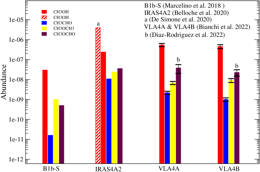
Figure 6: Abundance variation of CH₃OH, CH₃CHO, CH₃OCH₃,and CH₃OCHO obtained from interferometric observation. Black vertical lines represent the error bar.

4 Conclusion

Here, we analyze the ASAI large program data for five sources to understand the chemical and physical evolution of solar-type star-forming regions. We identify $\rm{CH_{3}OH,\ CH_{3}CHO,\ CH_{3}OCHO,\ C_{2}H_{5}OH,\ HCCCHO}$, $\rm{CH_{3}OCH_{3}}$, and CH₃CN in some of these sources we have considered. Observing these complex organic molecules in these four sources gave us a transparent view of evolutionary inheritance. The following are our initial findings in this article:

$\bullet$ An extensive study of the ASAI large program samples identifies many species with different transitions. We employ various LTE methods to measure excitation temperature and column density of a species. For the very first time in B1-b, we tentatively identify some transitions of $\rm{C_{2}H_{5}OH}$ with an upper limit of column density $1.0\times 10^{13}$ cm^-2.

$\bullet$ We noticed a comparatively enhanced column density of these species at the first hydrostatic core phase compared to the prestellar core. Moreover, no significant difference between class 0 (IRAS4A) and class I phase (SVS13A) has been observed. The two-class 0 objects IRAS4A and IRAS 16293-2422 show a significant difference (possibly because of the noticeable difference in luminosity). Abundances of the COMs gradually increase from the L1544 to IRAS16293-2422 and then decrease for SVS13A (Figure 1), except HCCCHO (upper limit). A similar trend is obtained by considering the beam dilution effect (Figure 1) and interferometric data from the literature (Figure 6).

$\bullet$ We found a trend in the obtained FWHM for a particular transition of methanol. It seems to increase steadily from L1544 (prestellar core) to SVS13A (class I). It also indicates a steady increase of FWHM with the luminosity of the sources.

Although the comparison focuses on only one source of each category, we cannot draw a clear conclusion about the observed trend. More observations of various sources in different stages of low-mass star formation with high spatial and angular resolution are needed to draw a reliable picture of the chemical evolution during the solar-type star formation process.

Appendix A Observed transitions

Table 6: Observed transitions toward some sources.

Species	Tag (Database)	Source	Frequency	Eup	Quantum No.	Aij	VLSR	Tpeak	FWHM	$\int$Tmb.dv
			(GHz)	(K)		(s-1)	(km.s-1)	(K)	(km.s-1)	(K.km.s-1)
CH3OH	32003(JPL)	L1544	84.521172	40.4	$5_{-1,0}$ - $4_{0,0}$	$1.97\times 10^{-6}$	7.240$\pm$ 0.010	0.017$\pm$ 0.001	0.441$\pm$ 0.024	0.008$\pm$ 0.001
(Methanol)			96.744545	20.1	$2_{0,0}$ - $1_{0,0}$	$3.41\times 10^{-6}$	7.160$\pm$ 0.020	0.109$\pm$ 0.001	0.358$\pm$ 0.004	0.042$\pm$ 0.001
			96.755501	28.0	$2_{1,0}$ - $1_{1,0}$	$2.62\times 10^{-6}$	7.070$\pm$ 0.010	0.013$\pm$ 0.001	0.416$\pm$ 0.029	0.006$\pm$ 0.001
			97.582798	21.5	$2_{1,-0}$ - $1_{1,-0}$	$2.6\times 10^{-6}$	7.180$\pm$ 0.010	0.019$\pm$ 0.001	0.428$\pm$ 0.021	0.009$\pm$ 0.001
		B1-b	96.739358	12.5	$2_{-1,0}$ - $1_{-1,0}$	$2.56\times 10^{-6}$	6.641$\pm$ 0.002	1.243$\pm$ 0.003	1.355$\pm$ 0.005	1.793$\pm$ 0.010
			96.741371	6.9	$2_{0,+0}$ - $1_{0,+0}$	$3.41\times 10^{-6}$	6.615$\pm$ 0.001	1.694$\pm$ 0.003	1.365$\pm$ 0.003	2.462$\pm$ 0.010
			96.744545	20.1	$2_{0,0}$ - $1_{0,0}$	$3.41\times 10^{-6}$	6.606$\pm$ 0.007	0.306$\pm$ 0.003	1.365$\pm$ 0.018	0.445$\pm$ 0.010
			96.755501	28.0	$2_{1,0}$ - $1_{1,0}$	$2.62\times 10^{-6}$	6.569$\pm$ 0.033	0.066$\pm$ 0.003	1.310$\pm$ 0.084	0.092$\pm$ 0.010
			108.893945	13.1	$0_{0,0}$ - $0_{1,-1}$	$1.47\times 10^{-5}$	6.565$\pm$0.005	0.377$\pm$ 0.003	1.371$\pm$ 0.013	0.550$\pm$ 0.009
			145.093754	27.0	$3_{0,0}$ - $2_{0,0}$	$1.23\times 10^{-5}$	6.671$\pm$ 0.003	0.479$\pm$ 0.003	0.950 $\pm$ 0.008	0.484$\pm$ 0.007
			145.103185	13.9	$3_{0,+0}$ - $2_{0,+0}$	$1.23\times 10^{-5}$	6.718$\pm$ 0.001	2.316$\pm$ 0.003	1.005$\pm$ 0.002	2.478$\pm$ 0.007
			157.270832	15.4	$1_{0,0}$ - $1_{-1,0}$	$2.21\times 10^{-5}$	6.513$\pm$0.002	0.896$\pm$ 0.003	1.012$\pm$ 0.004	0.965$\pm$ 0.007
			157.276019	20.1	$2_{0,0}$ - $2_{-1,0}$	$2.18\times 10^{-5}$	6.533$\pm$0.002	0.583$\pm$ 0.003	0.978$\pm$ 0.006	0.607$\pm$ 0.006
			165.050175	23.3	$1_{1,0}$ - $1_{0,0}$	$2.35\times 10^{-5}$	6.476$\pm$0.004	0.334$\pm$ 0.003	0.878$\pm$ 0.010	0.312$\pm$ 0.006
			165.061130	28.0	$2_{1,0}$ - $2_{0,0}$	$2.34\times 10^{-5}$	6.474$\pm$0.005	0.314$\pm$ 0.003	0.905$\pm$ 0.011	0.302$\pm$ 0.006
			165.099240	34.9	$3_{1,0}$ - $3_{0,0}$	$2.33\times 10^{-5}$	6.524$\pm$0.009	0.189$\pm$ 0.002	1.201$\pm$ 0.023	0.242$\pm$ 0.008
			170.060592	36.2	$3_{2,0}$ - $2_{1,0}$	2.55$\times 10^{-5}$	6.683$\pm$ 0.003	0.510$\pm$ 0.003	0.742$\pm$ 0.006	0.403$\pm$ 0.006
			213.427061	23.3	$1_{1,0}$ - $0_{0,0}$	$3.37\times 10^{-5}$	6.580$\pm$ 0.002	0.354$\pm$ 0.002	0.903$\pm$ 0.005	0.341$\pm$ 0.004
			254.015377	20.0	$2_{0,0}$ - $1_{-1,0}$	$1.90\times 10^{-5}$	6.621$\pm$ 0.002	0.427$\pm$ 0.001	1.035$\pm$ 0.005	0.471$\pm$ 0.004
			261.805675	28.0	$2_{1,0}$ - $1_{0,0}$	$5.57\times 10^{-5}$	6.623$\pm$ 0.002	0.354$\pm$ 0.001	1.005$\pm$ 0.005	0.379$\pm$ 0.003
		IRAS4A	96.755501	28.0	$2_{1,0}$ - $1_{1,0}$	$2.62\times 10^{-6}$	7.170$\pm$ 0.029	0.143$\pm$ 0.002	2.600$\pm$ 0.118	0.397$\pm$ 0.025
			108.893945	13.1	$0_{0,0}$ - $1_{-1,0}$	$1.47\times 10^{-6}$	7.402$\pm$ 0.011	0.335$\pm$ 0.002	2.446$\pm$ 0.046	0.871$\pm$ 0.022
			143.865795	28.3	$3_{1,+0}$ - $2_{1,+0}$	$1.07\times 10^{-5}$	7.279$\pm$ 0.010	0.313$\pm$ 0.002	2.697$\pm$ 0.042	0.899$\pm$ 0.019
			157.178987	47.9	$5_{0,0}$ - $5_{-1,0}$	$2.04\times 10^{-5}$	7.312$\pm$ 0.009	0.286$\pm$ 0.002	2.352$\pm$ 0.034	0.717$\pm$ 0.014
			165.050175	23.4	$1_{1,0}$ - $1_{0,0}$	$2.35\times 10^{-5}$	7.335$\pm$ 0.008	0.263$\pm$ 0.002	2.259$\pm$ 0.028	0.632$\pm$ 0.012
			165.061130	28.0	$2_{1,0}$ - $2_{0,0}$	$2.34\times 10^{-5}$	7.242$\pm$ 0.008	0.319$\pm$ 0.002	2.547$\pm$ 0.027	0.865$\pm$ 0.013
			165.099240	35.0	$3_{1,0}$ - $3_{0,0}$	$2.33\times 10^{-5}$	7.195$\pm$ 0.007	0.330$\pm$ 0.002	2.553$\pm$ 0.026	0.897$\pm$ 0.013
			213.427061	23.4	$1_{1,0}$ - $0_{0,0}$	$3.37\times 10^{-5}$	7.472$\pm$ 0.007	0.313$\pm$ 0.001	2.254$\pm$ 0.023	0.752$\pm$ 0.011
			230.027047	39.8	$3_{-2,0}$ - $4_{-1,0}$	$1.49\times 10^{-5}$	7.345$\pm$ 0.019	0.095$\pm$ 0.001	2.316$\pm$ 0.063	0.233$\pm$ 0.010
			254.015377	20.1	$2_{0,0}$ - $1_{-1,0}$	$1.90\times 10^{-5}$	7.073$\pm$ 0.005	0.329$\pm$ 0.001	2.030$\pm$ 0.015	0.711$\pm$ 0.008
			261.805675	28.0	$2_{1,0}$ - $1_{0,0}$	$5.57\times 10^{-5}$	7.095$\pm$ 0.004	0.420$\pm$ 0.001	2.275$\pm$ 0.014	1.016$\pm$ 0.009
			155.320895	140.6	$10_{0,0}$ - $10_{-1,0}$	$1.55\times 10^{-5}$	7.289$\pm$ 0.077	0.047$\pm$ 0.002	2.883$\pm$ 0.349	0.145$\pm$ 0.022
			155.997524	117.5	$9_{0,0}$ - $9_{-1,0}$	$1.67\times 10^{-5}$	7.355$\pm$ 0.076	0.060$\pm$ 0.002	4.328$\pm$ 0.278	0.278$\pm$ 0.025
			156.488902	96.6	$8_{8,0}$ - $8_{-1,0}$	$1.78\times 10^{-5}$	7.487$\pm$ 0.066	0.093$\pm$ 0.001	3.158$\pm$ 0.253	0.313$\pm$ 0.030
			156.828517	78.1	$7_{0,0}$ - $7_{-1,0}$	$1.88\times 10^{-5}$	7.305$\pm$ 0.031	0.125$\pm$ 0.002	3.467$\pm$ 0.163	0.460$\pm$ 0.027
			157.048617	61.8	$6_{0,0}$ - $6_{-1,0}$	$1.96\times 10^{-5}$	7.331$\pm$ 0.016	0.192$\pm$ 0.002	2.790$\pm$ 0.071	0.571$\pm$ 0.019
			165.678649	69.8	$6_{1,0}$ - $6_{0,0}$	$2.30\times 10^{-5}$	7.225$\pm$ 0.019	0.148$\pm$ 0.002	2.846$\pm$ 0.087	0.448$\pm$ 0.018
			166.169098	86.1	$7_{1,0}$ - $7_{0,0}$	$2.28\times 10^{-5}$	7.059$\pm$ 0.035	0.119$\pm$ 0.001	3.225$\pm$ 0.170	0.410$\pm$ 0.027
			241.879025	55.9	$5_{1,0}$ - $4_{1,0}$	$5.96\times 10^{-5}$	7.350$\pm$ 0.006	0.311$\pm$ 0.001	2.347$\pm$ 0.023	0.777$\pm$ 0.011
			251.738437	98.5	$6_{3,-0}$ - $6_{2,+0}$	$7.46\times 10^{-5}$	6.985$\pm$ 0.025	0.113$\pm$ 0.001	3.078$\pm$ 0.110	0.369$\pm$ 0.017
			251.866524	73.0	$4_{3,-0}$ - $4_{2,+0}$	$6.10\times 10^{-5}$	6.926$\pm$ 0.026	0.135$\pm$ 0.001	3.119$\pm$ 0.090	0.447$\pm$ 0.017
			251.917065	63.7	$3_{3,+0}$ - $3_{2,-0}$	$4.36\times 10^{-5}$	6.867$\pm$ 0.032	0.090$\pm$ 0.001	2.794$\pm$ 0.106	0.267$\pm$ 0.014
			251.984837	133.4	$8_{3,+0}$ - $8_{2,-0}$	$7.99\times 10^{-5}$	7.020$\pm$ 0.030	0.073$\pm$ 0.001	2.692$\pm$ 0.105	0.209$\pm$ 0.012
			252.090409	154.2	$9_{3,+0}$ - $9_{2,-0}$	$8.15\times 10^{-5}$	6.910$\pm$ 0.025	0.074$\pm$ 0.001	2.341$\pm$ 0.080	0.186$\pm$ 0.010
		SVS13A	85.568131	74.7	$6_{-2,0}$ - $7_{-1,0}$	$1.13\times 10^{-6}$	8.395$\pm$ 0.341	0.018$\pm$ 0.002	4.570$\pm$ 1.399	0.088$\pm$ 0.037
			96.755501	28.0	$2_{1,0}$ - $1_{1,0}$	$2.62\times 10^{-6}$	9.336$\pm$ 0.460	0.026$\pm$ 0.002	3.163$\pm$ 1.026	0.088$\pm$ 0.036
			111.289453	102.7	$7_{2,+0}$ - $8_{1,+0}$	$2.60\times 10^{-6}$	7.288$\pm$ 0.078	0.035$\pm$ 0.002	2.346$\pm$ 0.213	0.088$\pm$ 0.013
			143.865795	28.3	$3_{1,+0}$ - $2_{1,+0}$	$1.07\times 10^{-5}$	8.528$\pm$ 0.022	0.098$\pm$ 0.002	2.101$\pm$ 0.069	0.219$\pm$ 0.011
			156.602395	21.4	$2_{1,+0}$ - $3_{0,+0}$	$8.93\times 10^{-5}$	8.250$\pm$ 0.032	0.094$\pm$ 0.002	2.663$\pm$ 0.118	0.267$\pm$ 0.016
			218.440063	45.5	$4_{2,0}$ - $3_{1,0}$	$4.69\times 10^{-5}$	8.513$\pm$ 0.006	0.246$\pm$ 0.001	1.810$\pm$ 0.018	0.473$\pm$ 0.008
			229.758756	89.1	$8_{-1,0}$ - $7_{0,0}$	$4.19\times 10^{-5}$	8.146$\pm$ 0.025	0.155$\pm$ 0.001	3.380$\pm$ 0.092	0.557$\pm$ 0.020
			241.700159	47.9	$5_{0,0}$ - $4_{0,0}$	$6.04\times 10^{-5}$	8.086$\pm$ 0.017	0.184$\pm$ 0.001	2.744$\pm$ 0.053	0.538$\pm$ 0.014
			241.791352	34.8	$5_{0,+0}$ - $4_{0,+0}$	$6.05\times 10^{-5}$	8.169$\pm$ 0.004	0.430$\pm$ 0.001	1.680$\pm$ 0.010	0.768$\pm$ 0.007
			241.879025	55.9	$5_{1,0}$ - $4_{1,0}$	$5.96\times 10^{-5}$	8.051$\pm$ 0.029	0.166$\pm$ 0.001	3.094$\pm$ 0.085	0.547$\pm$ 0.019
			243.915788	49.7	$5_{1,-0}$ - $4_{1,-0}$	$5.97\times 10^{-5}$	8.444$\pm$ 0.012	0.163$\pm$ 0.001	2.659$\pm$ 0.043	0.461$\pm$ 0.011
			251.738437	98.5	$6_{3,-0}$ - $6_{0,+0}$	$7.46\times 10^{-5}$	8.463$\pm$ 0.037	0.089$\pm$ 0.001	3.380$\pm$ 0.197	0.320$\pm$ 0.023
			261.805675	28.0	$2_{1,0}$ - $1_{0,0}$	$5.57\times 10^{-5}$	8.915$\pm$ 0.009	0.154$\pm$ 0.001	1.691$\pm$ 0.024	0.277$\pm$ 0.006
			266.838148	57.1	$5_{2,0}$ - $4_{1,0}$	$7.74\times 10^{-5}$	8.357$\pm$ 0.009	0.197$\pm$ 0.001	2.003$\pm$ 0.028	0.420$\pm$ 0.009

Table 7: Observed transitions toward some sources.

Species	Tag (Database)	Source	Frequency	Eup	Quantum No.	Aij	VLSR	Tpeak	FWHM	$\int$Tmb.dv
			(GHz)	(K)		(s-1)	(km.s-1)	(K)	(km.s-1)	(K.km.s-1)
CH3CHO	44003 (JPL)	L1544	93.580909	15.7	51,5 - 41,4, (A)	$2.53\times 10^{-5}$	7.140$\pm$0.009	0.022$\pm$0.001	0.438$\pm$0.02	0.010$\pm$0.001
(Acetaldehyde)			93.595234	15.8	51,5 - 41,4, (E)	$2.53\times 10^{-5}$	7.190$\pm$0.007	0.024$\pm$0.001	0.342$\pm$0.017	0.009$\pm$0.001
			95.947437	13.9	50,5 - 40,4, (E)	$2.84\times 10^{-5}$	7.160$\pm$0.005	0.039$\pm$0.001	0.346$\pm$0.011	0.014$\pm$0.001
			95.963458	13.8	50,5 - 40,4, (A)	$2.84\times 10^{-5}$	7.180$\pm$0.006	0.041$\pm$0.001	0.437$\pm$0.013	0.019$\pm$0.001
			98.863313	16.6	51,4 - 41,3, (E)	$2.99\times 10^{-5}$	7.110$\pm$0.008	0.025$\pm$0.001	0.527$\pm$0.019	0.014$\pm$0.001
			98.900944	16.5	51,4 - 41,3, (A)	$2.99\times 10^{-5}$	7.170$\pm$0.008	0.02$\pm$0.001	0.34$\pm$0.02	0.007$\pm$0.001
		B1-b	93.580909	15.7	51,5 - 41,4, (A)	$2.53\times 10^{-5}$	6.570$\pm$0.040	0.051$\pm$0.003	1.428$\pm$0.110	0.078$\pm$0.010
			93.595234	15.8	51,5 - 41,4, (E)	$2.53\times 10^{-5}$	6.580$\pm$0.040	0.050$\pm$0.003	1.568$\pm$0.144	0.084$\pm$0.012
			95.963458	13.8	50,5 - 40,4, (A)	$2.84\times 10^{-5}$	6.660$\pm$0.030	0.073$\pm$0.003	1.461$\pm$0.080	0.114$\pm$0.011
			96.425614	22.9	52,4 - 42,3, (E)	$2.41\times 10^{-5}$	6.630$\pm$0.104	0.023$\pm$0.003	1.661$\pm$0.297	0.041$\pm$0.012
			96.475523	23.0	52,3 - 42,2, (E)	$2.42\times 10^{-5}$	6.520$\pm$0.083	0.022$\pm$0.003	0.973$\pm$0.199	0.022$\pm$0.008
			98.863313	16.6	51,4 - 41,3, (E)	$2.99\times 10^{-5}$	6.510$\pm$0.034	0.054$\pm$0.003	1.040$\pm$0.081	0.059$\pm$0.008
			98.900944	16.5	51,4 - 41,3, (A)	$2.99\times 10^{-5}$	6.550$\pm$0.040	0.049$\pm$0.003	1.249$\pm$0.100	0.066$\pm$0.009
			138.284995	28.9	71,6 - 61,5, (E)	$5.57\times 10^{-5}$	6.820$\pm$0.027	0.054$\pm$0.003	0.870$\pm$0.063	0.050$\pm$0.006
			138.319628	28.8	71,6 - 61,5, (A)	$8.57\times 10^{-5}$	6.650$\pm$0.031	0.048$\pm$0.003	0.775$\pm$0.072	0.039$\pm$0.006
			152.635193	33.1	80,8 - 70,7, (A)	$1.18\times 10^{-4}$	6.280$\pm$0.049	0.034$\pm$0.003	0.750$\pm$0.116	0.027$\pm$0.006
		IRAS4A	74.891677	11.2	41,4 - 31,3, (A)	$1.24\times 10^{-5}$	6.840$\pm$0.050	0.051$\pm$0.003	2.641$\pm$0.216	0.144$\pm$0.021
			74.924133	11.3	41,4 - 31,3, (E)	$1.24\times 10^{-5}$	7.030$\pm$0.070	0.050$\pm$0.003	2.375$\pm$0.225	0.126$\pm$0.019
			76.878952	9.2	40,4 - 30,3, (A)	$1.43\times 10^{-5}$	7.140$\pm$0.060	0.061$\pm$ 0.003	2.332$\pm$ 0.185	0.152$\pm$ 0.019
			77.038601	18.3	42,3 - 32,2, (A)	$1.08\times 10^{-5}$	6.960$\pm$0.190	0.022$\pm$ 0.003	2.653$\pm$ 0.507	0.063$\pm$ 0.021
			77.218291	18.3	42,2 - 32,1, (A)	$1.09\times 10^{-5}$	6.510$\pm$0.150	0.029$\pm$ 0.003	2.708$\pm$ 0.408	0.082$\pm$ 0.021
			79.099313	11.8	41,3 - 31,2, (E)	$1.46\times 10^{-5}$	7.010$\pm$0.070	0.059$\pm$ 0.003	2.299$\pm$ 0.207	0.144$\pm$ 0.020
			93.580909	15.7	51,5 - 41,4, (A)	$2.53\times 10^{-5}$	7.320$\pm$0.050	0.065$\pm$ 0.003	2.298$\pm$ 0.143	0.158$\pm$ 0.016
			93.595234	15.8	51,5 - 41,4, (E)	$2.53\times 10^{-5}$	7.440$\pm$0.050	0.062$\pm$ 0.003	2.343$\pm$ 0.159	0.155$\pm$ 0.017
			95.947437	13.9	50,5 - 40,4, (E)	$2.84\times 10^{-5}$	7.390$\pm$0.030	0.081$\pm$ 0.003	2.277$\pm$ 0.102	0.197$\pm$ 0.016
			96.274252	22.9	52,4 - 42,3, (A)	$2.41\times 10^{-5}$	7.330$\pm$0.070	0.037$\pm$ 0.003	2.148$\pm$ 0.222	0.085$\pm$ 0.015
			96.425614	22.9	52,4 - 42,3, (E)	$2.41\times 10^{-5}$	7.540$\pm$0.100	0.031$\pm$ 0.003	2.406$\pm$ 0.315	0.078$\pm$ 0.017
			96.475523	23.0	52,3 - 42,2, (E)	$2.42\times 10^{-5}$	7.170$\pm$0.090	0.036$\pm$ 0.003	2.357$\pm$ 0.248	0.092$\pm$ 0.016
			98.863313	16.6	51,4 - 41,3, (E)	$2.99\times 10^{-5}$	7.360$\pm$0.040	0.076$\pm$ 0.003	2.242$\pm$ 0.115	0.182$\pm$ 0.016
			112.248716	21.1	61,6 - 51,5, (A)	$4.50\times 10^{-5}$	7.290$\pm$0.050	0.065$\pm$ 0.002	2.559$\pm$ 0.148	0.178$\pm$ 0.017
			112.254508	21.2	61,6 - 51,5, (E)	$4.50\times 10^{-5}$	7.270$\pm$0.060	0.062$\pm$ 0.002	3.061$\pm$ 0.199	0.203$\pm$ 0.021
			133.830491	25.8	70,7 - 60,6, (E)	$7.91\times 10^{-5}$	7.330$\pm$0.020	0.084$\pm$ 0.002	2.113$\pm$ 0.068	0.189$\pm$ 0.011
			138.284995	28.9	71,6 - 61,5, (E)	$8.57\times 10^{-5}$	7.660$\pm$0.030	0.067$\pm$ 0.002	2.314$\pm$ 0.088	0.165$\pm$ 0.011
			138.319628	28.8	71,6 - 61,5, (A)	$8.57\times 10^{-5}$	7.510$\pm$0.030	0.063$\pm$ 0.002	2.541$\pm$ 0.102	0.171$\pm$ 0.012
			152.635193	33.1	80,8 - 70,7, (A)	$1.18\times 10^{-4}$	7.480$\pm$0.020	0.077$\pm$ 0.002	2.105$\pm$ 0.064	0.173$\pm$ 0.010
			155.342088	42.5	82,6 - 72,5, (A)	$1.17\times 10^{-4}$	7.230$\pm$0.040	0.053$\pm$ 0.002	2.193$\pm$ 0.105	0.123$\pm$ 0.010
			168.093444	42.6	91,9 - 81,8, (A)	$1.57\times 10^{-4}$	7.390$\pm$0.030	0.069$\pm$ 0.002	2.622$\pm$ 0.095	0.192$\pm$ 0.012
			208.228560	60.5	110,11 - 100,10, (E)	$3.05\times 10^{-4}$	7.360$\pm$0.030	0.054$\pm$ 0.002	2.451$\pm$ 0.099	0.140$\pm$ 0.010
			211.273792	70.0	112,10 - 102,9, (E)	$3.09\times 10^{-4}$	7.410$\pm$0.020	0.063$\pm$0.001	1.645$\pm$0.077	0.110$\pm$ 0.008
			212.257139	81.4	113,9 - 103,8, (A)	$3.00\times 10^{-4}$	7.530$\pm$0.020	0.043$\pm$ 0.002	1.306$\pm$ 0.059	0.060$\pm$ 0.005
			214.845041	70.6	112,9 - 102,8, (A)	$3.25\times 10^{-4}$	7.470$\pm$0.020	0.055$\pm$ 0.001	1.771$\pm$ 0.080	0.103$\pm$ 0.007
			216.630234	64.8	111,10 - 101,9, (A)	$3.41\times 10^{-4}$	7.470$\pm$0.020	0.070$\pm$ 0.002	1.409$\pm$ 0.065	0.105$\pm$ 0.007
			223.660602	72.2	121,12 - 111,11, (A)	$3.77\times 10^{-4}$	7.360$\pm$0.020	0.066$\pm$ 0.002	2.027$\pm$ 0.061	0.143$\pm$ 0.008
			242.106020	83.9	131,13 - 121,12, (E)	$4.81\times 10^{-4}$	7.130$\pm$0.040	0.051$\pm$ 0.001	2.123$\pm$ 0.108	0.116$\pm$ 0.009
			250.829158	120.3	134,9 - 124,8, (E)	$4.87\times 10^{-4}$	7.060$\pm$0.030	0.044$\pm$ 0.002	1.626$\pm$ 0.092	0.077$\pm$ 0.007
			250.934558	104.6	133,11 - 123,10, (A)	$5.10\times 10^{-4}$	7.180$\pm$0.030	0.042$\pm$ 0.002	1.497$\pm$ 0.093	0.067$\pm$ 0.007
			251.489286	104.7	133,10 - 123,9, (A)	$5.14\times 10^{-4}$	6.850$\pm$0.030	0.055$\pm$ 0.001	1.823$\pm$ 0.079	0.106$\pm$ 0.007
			254.827152	94.1	132,11 - 122,10, (E)	$5.51\times 10^{-4}$	7.260$\pm$0.050	0.041$\pm$ 0.001	2.027$\pm$ 0.132	0.089$\pm$ 0.009
			255.326968	88.4	131,12 - 121,11, (E)	$5.64\times 10^{-4}$	7.250$\pm$0.030	0.043$\pm$ 0.001	1.884$\pm$ 0.115	0.087$\pm$ 0.008
			262.960097	95.7	140,14 - 130,13, (E)	$6.19\times 10^{-4}$	6.730$\pm$0.030	0.056$\pm$ 0.001	1.770$\pm$ 0.076	0.105$\pm$ 0.007
		SVS13A	205.170685	61.4	111,11 - 101,10, (A)	$2.90\times 10^{-4}$	8.560$\pm$0.030	0.039$\pm$0.002	1.550$\pm$ 0.094	0.064$\pm$0.007
			211.243042	69.9	112,10 - 102,9, (A)	$3.09\times 10^{-4}$	8.470$\pm$0.040	0.040$\pm$ 0.001	1.972$\pm$ 0.141	0.083$\pm$ 0.009
			211.273792	70.0	112,10 - 102,9, (E)	$3.09\times 10^{-4}$	8.790$\pm$ 0.050	0.040$\pm$ 0.001	1.925$\pm$ 0.158	0.081$\pm$ 0.010
			216.581930	64.8	111,10 - 101,9, (E)	$3.41\times 10^{-4}$	8.050$\pm$ 0.050	0.044$\pm$ 0.001	1.970$\pm$ 0.149	0.092$\pm$ 0.010
			230.301923	81.0	122,11 - 112,10, (A)	$4.04\times 10^{-4}$	8.550$\pm$ 0.030	0.036$\pm$ 0.001	1.630$\pm$ 0.104	0.062$\pm$ 0.007
			242.106020	83.9	131,13 - 121,12, (E)	$4.81\times 10^{-4}$	8.080$\pm$ 0.030	0.053$\pm$ 0.001	1.574$\pm$ 0.101	0.090$\pm$ 0.008
			251.489286	104.7	133,10 - 123,9, (A)	$5.14\times 10^{-4}$	8.290$\pm$ 0.030	0.030$\pm$ 0.002	1.022$\pm$ 0.076	0.032$\pm$ 0.004

Table 8: Observed transitions toward some sources.

Species	Tag (Database)	Source	Frequency	Eup	Quantum No.	Aij	VLSR	Tpeak	FWHM	$\int$Tmb.dv
			(GHz)	(K)		(s-1)	(km.s-1)	(K)	(km.s-1)	(K.km.s-1)
CH3OCHO	60003 (JPL)	B1-b	88.851607	17.9	71,6 - $6_{1,5}$ (A)	$9.82\times 10^{-6}$	6.560$\pm$0.217	0.013$\pm$0.003	1.915$\pm$0.635	0.026$\pm$0.014
(Methyl formate)			90.145723	19.7	$7_{2,5}$ - $6_{2,4}$ (E)	$9.74\times 10^{-6}$	6.680$\pm$0.1806	0.013$\pm$0.003	1.585$\pm$0.490	0.022$\pm$0.011
			90.156473	19.6	$7_{2,5}$ - $6_{2,4}$ (A)	$9.75\times 10^{-6}$	6.570$\pm$0.169	0.014$\pm$0.003	1.514$\pm$0.438	0.023 $\pm$0.011
			100.294604	27.4	$8_{3,5}$ - $7_{3,4}$ (E)	$1.26\times 10^{-5}$	6.510$\pm$0.162	0.012$\pm$0.003	1.172$\pm$0.404	0.016$\pm$0.009
			100.482241	22.8	$8_{1,7}$ - $7_{1,6}$ (E)	$1.43\times 10^{-5}$	6.730$\pm$0.131	0.018$\pm$0.003	1.331$\pm$0.348	0.026$\pm$0.011
			103.478663	24.6	$8_{2,6}$ - $7_{2,5}$ (A)	$1.52\times 10^{-5}$	6.610$\pm$0.179	0.013$\pm$0.003	1.636$\pm$0.457	0.022$\pm$0.011
		IRAS4A	129.296357	36.4	$10_{2,8}$ - $9_{2,7}$ (E)	$3.06\times 10^{-5}$	7.180$\pm$0.060	0.025$\pm$0.002	1.588$\pm$0.161	0.042$\pm$0.007
			132.928736	40.4	$11_{1,1}$ - $10_{1,9}$ (A)	$3.36\times 10^{-5}$	7.000$\pm$0.140	0.016$\pm$0.001	2.210$\pm$0.429	0.039$\pm$0.011
			135.921949	55.6	$11_{5,7}$ - $10_{5,6}$ (A)	$2.95\times 10^{-5}$	7.340$\pm$0.050	0.027$\pm$0.002	1.200$\pm$0.131	0.034$\pm$0.007
			141.044354	47.5	$12_{2,11}$ - $11_{2,10}$ (A)	$4.02\times 10^{-5}$	7.230$\pm$0.050	0.028$\pm$0.002	1.342$\pm$0.139	0.040$\pm$0.007
			158.693722	59.6	$13_{3,11}$ - $12_{3,10}$ (E)	$5.61\times 10^{-5}$	7.430$\pm$0.090	0.022$\pm$0.002	2.402$\pm$0.306	0.057$\pm$0.011
			158.704392	59.6	$13_{3,11}$ - $12_{3,10}$ (A)	$5.61\times 10^{-5}$	7.220$\pm$0.090	0.023$\pm$0.002	2.153$\pm$0.313	0.052$\pm$0.011
			200.956372	97.5	$16_{5,11}$ - $15_{5,10}$ (A)	$1.10\times 10^{-4}$	7.030$\pm$0.020	0.045$\pm$0.002	1.110$\pm$0.065	0.054$\pm$0.005
			206.619476	89.2	$16_{3,13}$ - $15_{3,12}$ (A)	$1.28\times 10^{-4}$	7.630$\pm$0.030	0.038$\pm$0.002	1.306$\pm$0.095	0.052$\pm$0.006
			216.216539	109.3	$19_{1,18}$ - $18_{1,17}$ (A)	$1.49\times 10^{-4}$	7.460$\pm$0.030	0.030$\pm$0.002	1.322$\pm$0.094	0.042$\pm$0.005
			228.628876	118.8	$18_{5,13}$ - $17_{5,12}$ (E)	$1.66\times 10^{-4}$	7.190$\pm$0.020	0.049$\pm$0.002	1.172$\pm$0.068	0.061$\pm$0.005
			240.021140	122.3	$19_{3,16}$ - $18_{3,15}$ (E)	$2.01\times 10^{-4}$	7.140$\pm$0.032	0.036$\pm$0.002	1.325$\pm$0.078	0.051$\pm$0.005
			247.044146	139.9	$21_{3,19}$ - $20_{3,18}$ (E)	$2.21\times 10^{-4}$	7.380$\pm$0.035	0.033$\pm$0.002	0.964$\pm$0.084	0.034$\pm$0.005
			249.578117	148.7	$20_{6,15}$ - $19_{6,14}$ (E)	$2.14\times 10^{-4}$	7.230$\pm$0.032	0.031$\pm$0.002	1.224$\pm$0.075	0.041$\pm$0.005
		SVS13A	100.490682	22.7	$8_{1,7}$ - $7_{1,6}$ (A)	$1.43\times 10^{-5}$	8.830$\pm$0.230	0.015$\pm$0.002	2.474$\pm$0.779	0.040$\pm$0.018
			164.205978	64.9	$13_{4,9}$ - $12_{4,8}$ (E)	$5.98\times 10^{-5}$	8.960$\pm$0.030	0.040$\pm$0.002	1.453$\pm$0.096	0.061$\pm$0.007
			210.463200	123.0	177,10 - $16_{7,9}$ (A)	$1.17\times 10^{-4}$	8.750$\pm$0.030	0.030$\pm$0.002	1.350$\pm$0.092	0.043$\pm$0.005
			218.280900	99.7	$17_{3,14}$ - $16_{3,13}$ (E)	$1.51\times 10^{-4}$	8.620$\pm$0.040	0.037$\pm$0.001	2.472$\pm$0.168	0.098$\pm$0.010
			222.421489	143.5	$18_{8,10}$ - $17_{8,9}$ (E)	$1.33\times 10^{-4}$	8.630$\pm$0.030	0.037$\pm$0.001	1.996$\pm$0.109	0.079$\pm$0.007
			269.078001	168.8	$24_{2,23}$ - $23_{2,22}$ (E)	$2.90\times 10^{-4}$	8.570$\pm$0.020	0.048$\pm$0.001	1.700$\pm$0.062	0.086$\pm$0.006
$\rm{C_{2}H_{5}OH}$ v=0	46524 (CDMS)	IRAS4A	129.6657634	23.8	$5_{3,2}$ - $5_{2,3}$,vt=2 - 2	$1.14\times 10^{-5}$	6.890$\pm$0.068	0.015$\pm$0.002	1.140$\pm$0.172	0.019 $\pm$0.005
(Ethanol)			133.3234312	23.8	$7_{1,7}$ - $6_{0,6}$,vt=2 - 2	$1.83\times 10^{-5}$	7.620$\pm$0.080	0.026$\pm$0.002	2.042$\pm$0.231	0.056$\pm$0.010
			148.3040357	58.15	$11_{1,10}$ - $10_{2,9}$,vt=2 - 2	$1.21\times 10^{-5}$	7.580$\pm$0.060	0.017$\pm$0.002	0.981$\pm$0.165	0.018 $\pm$0.005
			159.4140526	101.1	$9_{1,8}$ - $8_{1,7}$,vt=1 - 1	$3.65\times 10^{-5}$	7.230$\pm$0.050	0.021$\pm$0.002	0.696$\pm$0.125	0.016$\pm$0.005
			205.4584717	64.0	$12_{1,12}$ - $11_{0,11}$,vt=2 - 2	$8.04\times 10^{-5}$	7.510$\pm$0.050	0.031$\pm$0.002	1.663$\pm$0.132	0.054$\pm$0.007
			209.8652009	132.9	$12_{3,9}$ - $11_{3,8}$,vt=0 - 0	$8.01\times 10^{-5}$	7.170$\pm$0.030	0.023$\pm$0.003	0.583$\pm$0.076	0.015$\pm$0.003
			227.8919226	140.0	$13_{1,12}$ - $12_{1,11}$,vt=1 - 1	$1.12\times 10^{-4}$	7.210$\pm$0.020	0.029$\pm$0.002	0.636$\pm$0.062	0.020$\pm$0.004
			230.9913834	85.5	$14_{0,14}$ - $13_{1,13}$,vt=2 - 2	$1.20\times 10^{-4}$	7.16$\pm$0.02	0.044 $\pm$0.002	0.957$\pm$0.064	0.045$\pm$0.005
		SVS13A	84.5958861	13.4	$4_{2,3}$ - $4_{1,4}$,vt= 2- 2	$3.25\times 10^{--6}$	8.640$\pm$0.170	0.012$\pm$0.002	1.353$\pm$0.475	0.017$\pm$0.009
			130.2463048	19.7	$4_{3,1}$ - $4_{2,2}$,vt=2 - 2	$9.98\times 10^{-6}$	8.680$\pm$0.050	0.016$\pm$0.002	0.719$\pm$0.117	0.012$\pm$0.004
			153.4842039	99.1	$9_{2,8}$ - $8_{1,8}$,vt=0 - 1	$4.17\times 10^{-5}$	8.300$\pm$0.060	0.017$\pm$0.002	0.861$\pm$0.150	0.015$\pm$0.005
			205.4584717	64.0	$12_{1,12}$ - $11_{0,11}$,vt=2 - 2	$8.04\times 10^{-5}$	8.770$\pm$0.020	0.037$\pm$0.002	0.884$\pm$0.066	0.035$\pm$0.005
			244.633959	151.7	$14_{1,13}$ - $13_{1,12}$,vt=1 - 1	$1.42\times 10^{-4}$	8.770$\pm$0.030	0.022$\pm$0.002	0.705$\pm$0.091	0.016$\pm$0.004
			270.4440852	32.6	$5_{4,2}$ - $4_{3,1}$,vt=2 - 2	$1.59\times 10^{-4}$	8.720$\pm$0.010	0.042$\pm$0.002	0.811$\pm$0.044	0.036$\pm$0.004
$\rm{HCCCHO}$	54007 (JPL)	L1544	83.775816	20.1	90,9 - 80,8	1.85$\times$10-5	7.130 $\pm$0.019	0.011$\pm$0.001	0.393$\pm$0.046	0.004$\pm$0.001
(Propynal)			99.039070	7.44	41,4 - 30,3	1.13$\times$10-6	7.110 $\pm$ 0.020	0.012$\pm$ 0.001	0.432$\pm$0.045	0.005$\pm$0.001
			102.298030	29.5	110,11 - 100,10	3.40$\times$10-5	7.080$\pm$ 0.020	0.013$\pm$0.001	0.486$\pm$0.042	0.007$\pm$0.001
$\rm{CH_{3}OCH_{3}}$	46514 (CDMS)	L1544	99.324362	10.2	41,4 - 30,3 (EA)	5.53$\times$ 10-6	$\cdots$	$\cdots$	$\cdots$	$\cdots$
(Dimethyl ether)			99.324364	10.2	41,4 - 30,3 (AE)	5.53$\times$ 10-6	$\cdots$	$\cdots$	$\cdots$	$\cdots$
			99.325217	10.2	41,4 - 30,3 (EE)	5.53$\times$ 10-6	$\cdots$	$\cdots$	$\cdots$	$\cdots$
			99.326072	10.2	41,4 - 30,3 (AA)	5.53$\times$ 10-6	$\cdots$	$\cdots$	$\cdots$	$\cdots$
		B1-b	99.324362	10.2	41,4 - 30,3 (EA)	5.53$\times$ 10-6	$\cdots$	$\cdots$	$\cdots$	$\cdots$
			99.324364	10.2	41,4 - 30,3 (AE)	5.53$\times$ 10-6	$\cdots$	$\cdots$	$\cdots$	$\cdots$
			99.325217	10.2	41,4 - 30,3 (EE)	5.53$\times$ 10-6	$\cdots$	$\cdots$	$\cdots$	$\cdots$
			99.326072	10.2	41,4 - 30,3 (AA)	5.53$\times$ 10-6	$\cdots$	$\cdots$	$\cdots$	$\cdots$
		IRAS4A	162.529582	33.0	81,8 - 70,7, (EE)	2.67$\times$10-5	7.180$\pm$0.060	0.041$\pm$0.002	2.668$\pm$0.287	0.117$\pm$0.017
			209.515644	59.3	111,11 - 100,10, (EE)	6.40$\times$10-5	7.050$\pm$0.020	0.053$\pm$0.001	1.640$\pm$0.076	0.093$\pm$0.007
			225.599126	69.5	121,12 - 110,11, (EE)	8.25$\times$10-5	7.420$\pm$0.020	0.068$\pm$0.001	1.360$\pm$0.063	0.099$\pm$0.007
			241.946542	81.1	131,13 - 120,12, (EE)	1.05$\times$10-4	7.370$\pm$0.040	0.047$\pm$0.001	2.025$\pm$0.129	0.103$\pm$0.009
$\rm{CH_{3}CN}$	41001 (JPL)	L1544	91.985314	20.4	51 - 41	6.08$\times$ 10-5	7.280$\pm$0.002	0.087$\pm$0.001	0.542 $\pm$ 0.006	0.050$\pm$0.001
(Methyl cyanide)			91.987087	13.2	50 - 40	6.33$\times$ 10-5	7.282$\pm$0.002	0.127 $\pm$0.001	0.505$\pm$0.004	0.068$\pm$0.001
		B1-b	91.985314	20.4	51 - 41	6.08$\times$ 10-5	6.719$\pm$ 0.143	0.018$\pm$0.003	1.731 $\pm$0.388	0.034 $\pm$0.013
			91.987087	13.2	50 - 40	6.33$\times$ 10-5	6.654$\pm$ 0.090	0.029$\pm$0.003	1.846$\pm$0.253	0.058$\pm$0.013
		IRAS4A	73.588799	16.0	$4_{1}$ - $3_{1}$	2.97$\times$ 10-5	6.726 $\pm$ 0.141	0.043 $\pm$ 0.003	2.758 $\pm$ 0.472	0.127 $\pm$ 0.029
			73.590218	8.8	$4_{0}$ - 30	3.17$\times$ 10-5	7.025 $\pm$ 0.121	0.055 $\pm$ 0.003	2.858$\pm$ 0.480	0.169$\pm$ 0.036
			91.979994	41.8	$5_{2}$ - $4_{2}$	5.32$\times$ 10-5	7.071$\pm$ 0.170	0.029$\pm$ 0.002	2.661 $\pm$ 0.853	0.082 $\pm$ 0.033
			91.985314	20.4	$5_{1}$ - $4_{1}$	6.08$\times$ 10-5	6.943$\pm$ 0.089	0.054$\pm$ 0.002	3.119 $\pm$ 0.399	0.179$\pm$ 0.031
			91.987087	13.2	$5_{0}$ - $4_{0}$	6.33$\times$ 10-5	7.083$\pm$ 0.056	0.078$\pm$ 0.002	2.658 $\pm$ 0.239	0.221 $\pm$ 0.027
			110.364353	82.8	$6_{3}$ - $5_{3}$	8.33$\times$ 10-5	7.297$\pm$ 0.051	0.039 $\pm$ 0.003	1.737$\pm$ 0.131	0.072$\pm$ 0.010
			110.3813720	25.7	$6_{1}$ - $5_{1}$	1.08$\times$ 10-4	7.406 $\pm$ 0.055	0.072$\pm$ 0.002	3.018 $\pm$ 0.235	0.233 $\pm$ 0.025
			110.383499	18.5	$6_{0}$ - $5_{0}$	1.11$\times$ 10-4	7.299$\pm$ 0.056	0.076$\pm$ 0.002	3.180$\pm$ 0.253	0.258$\pm$ 0.028
			128.757030	89.0	$7_{3}$ - $6_{3}$	1.46$\times$ 10-4	7.052$\pm$ 0.135	0.029$\pm$ 0.001	2.902$\pm$ 0.464	0.089$\pm$ 0.018
			128.769436	53.3	$7_{2}$ - $6_{2}$	1.64$\times$ 10-4	6.812$\pm$ 0.072	0.043$\pm$ 0.001	3.134 $\pm$ 0.266	0.144$\pm$ 0.017
			128.776881	31.9	$7_{1}$ - $6_{1}$	1.75$\times$ 10-4	6.675$\pm$ 0.045	0.078 $\pm$ 0.001	2.941$\pm$ 0.135	0.244$\pm$ 0.015
			128.779363	24.7	$7_{0}$ - $6_{0}$	1.78$\times$ 10-4	6.990$\pm$ 0.050	0.092$\pm$ 0.001	2.926 $\pm$ 0.209	0.285$\pm$ 0.024
			147.163244	60.4	$8_{2}$ - $7_{2}$	2.52$\times$ 10-4	6.898$\pm$ 0.062	0.039$\pm$ 0.002	2.349$\pm$ 0.211	0.098$\pm$ 0.013
			147.171751	38.9	$8_{1}$ - $7_{1}$	2.64$\times$ 10-4	6.854$\pm$ 0.051	0.070$\pm$ 0.002	3.131$\pm$ 0.186	0.232$\pm$ 0.019
			147.174588	31.8	$8_{0}$ - $7_{0}$	2.69$\times$ 10-4	7.147$\pm$ 0.031	0.087$\pm$ 0.002	2.787$\pm$ 0.134	0.258$\pm$ 0.017
			165.540377	104.0	$9_{3}$ - $8_{3}$	3.42$\times$ 10-4	6.815$\pm$ 0.113	0.039 $\pm$ 0.001	3.176$\pm$ 0.399	0.131$\pm$ 0.021
			165.556321	68.3	$9_{2}$ - $8_{2}$	3.66$\times$ 10-4	7.192$\pm$ 0.044	0.042$\pm$ 0.002	2.204$\pm$ 0.134	0.098$\pm$ 0.010
			165.565891	46.9	$9_{1}$ - $8_{1}$	3.80$\times$ 10-4	7.189$\pm$ 0.036	0.070$\pm$ 0.002	2.912$\pm$ 0.141	0.216$\pm$ 0.015
			165.569081	39.7	$9_{0}$ - $8_{0}$	3.85$\times$ 10-4	7.183$\pm$ 0.030	0.078$\pm$ 0.002	2.656$\pm$ 0.122	0.220$\pm$ 0.014
			202.320442	122.6	$11_{3}$ - $10_{3}$	6.56$\times$ 10-4	7.101$\pm$ 0.027	0.059 $\pm$ 0.002	2.086$\pm$ 0.077	0.131$\pm$ 0.008
			220.709016	133.2	$12_{3}$ - $11_{3}$	8.66$\times$ 10-4	7.324 $\pm$ 0.051	0.049 $\pm$ 0.001	2.570 $\pm$ 0.192	0.135 $\pm$ 0.014

Table 9: Observed transitions toward some sources.

Species	Tag (Database)	Source	Frequency	Eup	Quantum No.	Aij	VLSR	Tpeak	FWHM	$\int$Tmb.dv
			(GHz)	(K)		(s-1)	(km.s-1)	(K)	(km.s-1)	(K.km.s-1)
		SVS13A	91.979994	41.8	$5_{2}$ - $4_{2}$	3.32$\times$ 10-5	7.918$\pm$ 0.569	0.020 $\pm$ 0.002	3.205$\pm$ 1.528	0.067 $\pm$ 0.038
			91.985314	20.4	$5_{1}$ - $4_{1}$	6.08$\times$ 10-5	8.428$\pm$ 0.133	0.029$\pm$ 0.002	2.762$\pm$ 0.588	0.086$\pm$ 0.024
			91.987087	13.2	$5_{0}$ - $4_{0}$	36.33$\times$ 10-5	8.580$\pm$ 0.078	0.035$\pm$ 0.002	2.366$\pm$ 0.272	0.088$\pm$ 0.015
			110.364353	82.8	$6_{3}$ - $5_{3}$	8.33$\times$ 10-5	8.808$\pm$ 0.145	0.025$\pm$ 0.002	3.050$\pm$ 0.596	0.080$\pm$ 0.022
			110.374989	47.1	$6_{2}$ - $5_{2}$	9.87$\times$ 10-5	8.531$\pm$ 0.177	0.030$\pm$ 0.002	3.366 $\pm$ 1.134	0.109 $\pm$ 0.043
			110.381372	25.7	$6_{1}$ - $5_{1}$	1.08$\times$ 10-4	8.284$\pm$ 0.083	0.042$\pm$ 0.002	2.540$\pm$ 0.245	0.114$\pm$ 0.016
			110.383499	18.5	$6_{0}$ - $5_{0}$	1.11$\times$ 10-4	8.315$\pm$ 0.102	0.033$\pm$ 0.002	2.649$\pm$ 0.332	0.093$\pm$ 0.017
			128.776881	31.8	$7_{1}$ - $6_{1}$	1.75$\times$ 10-4	8.392$\pm$ 0.034	0.050$\pm$ 0.002	1.719$\pm$ 0.094	0.092$\pm$ 0.008
			128.779363	24.7	$7_{0}$ - $6_{0}$	1.78$\times$ 10-4	8.280$\pm$ 0.036	0.050$\pm$ 0.001	1.990$\pm$ 0.107	0.105$\pm$ 0.009
			147.171751	38.9	$8_{1}$ - $7_{1}$	2.64$\times$ 10-4	8.162$\pm$ 0.051	0.062 $\pm$ 0.002	2.533 $\pm$ 0.164	0.167$\pm$ 0.015
			165.565891	46.9	$9_{1}$ - $8_{1}$	3.80$\times$ 10-4	8.343$\pm$ 0.030	0.091 $\pm$ 0.002	2.307$\pm$ 0.099	0.223 $\pm$ 0.013
			220.709016	133.2	$12_{3}$ - $11_{3}$	8.66$\times$ 10-4	8.576$\pm$ 0.033	0.077 $\pm$ 0.001	3.238$\pm$ 0.136	0.265 $\pm$ 0.016
			220.730260	97.4	$12_{2}$ - $11_{2}$	8.98$\times$ 10-4	8.363$\pm$ 0.051	0.071$\pm$ 0.001	3.900$\pm$ 0.236	0.294$\pm$ 0.023
			220.743010	76.0	$12_{1}$ - $11_{1}$	9.18$\times$ 10-4	8.300$\pm$ 0.028	0.088$\pm$ 0.001	2.951$\pm$ 0.110	0.278$\pm$ 0.014
			220.747261	68.9	$12_{0}$ - $11_{0}$	9.24$\times$ 10-4	8.382$\pm$ 0.040	0.090$\pm$ 0.001	3.907$\pm$ 0.186	0.373$\pm$ 0.023
			239.119504	108.9	$13_{2}$ - $12_{2}$	1.15$\times$ 10-3	8.209$\pm$ 0.040	0.091$\pm$ 0.001	2.952$\pm$ 0.139	0.285$\pm$ 0.017
			257.527383	92.7	$14_{0}$ - $13_{0}$	1.48$\times$ 10-3	8.426$\pm$ 0.059	0.092$\pm$ 0.001	4.037$\pm$ 0.321	0.394$\pm$ 0.036

Appendix B Upper limit estimation

For some species, we were unable to identify suitable and multiple transitions to estimate the column density by rotation diagram and MCMC method. In Table 10, we note the estimated upper limits of column density for these species. The input parameters used for this estimation are also noted.

Table 10: Estimated upper limit of column density

Molecules	Source	Frequency	Quantum No.	Eup	Aij	Ntot	Tk
		(GHz)		(K)	(s-1)	(cm-2)	(K)
CH3OCHO	L1544	90.227659	80,8 - 70,7, (E)	20.1	$1.05\times 10^{-5}$	$3.7\times 10^{12}$	10.0
C2H5OH	B1-b	131.502781	63,4 - 62,5, vt = $2-2$	28.9	$1.27\times 10^{-5}$	$1.0\times 10^{13}$	20.0
HCCCHO	B1-b	93.0432843	100,10 - 90,9	24.6	$2.55\times 10^{-5}$	$2.56\times 10^{12}$	20.0
	IRAS4A	111.53912	120,12 - 110,11	34.8	$4.43\times 10^{-5}$	$3.9\times 10^{12}$	40.0
	SVS13A	236.6916499	214,17 - 223,20	152.0	$4.96\times 10^{-6}$	$4.00\times 10^{14}$	100.0

Appendix C Rotational diagram

For the optically thin transitions, upper state column density (N${}_{u}^{thin}$) can be expressed as (Goldsmith & Langer, 1999),

$$\frac{N_{u}^{thin}}{g_{u}}=\frac{3k_{B}\int{T_{mb}dV}}{8\pi^{3}\nu S\mu^{2}},$$ (C1)

where g_u is the degeneracy of the upper state, k_B is the Boltzmann constant, $\rm{\int T_{mb}dV}$ is the integrated intensity, $\nu$ is the rest frequency, $\mu$ is the electric dipole moment, and S is the transition line strength. Under the LTE conditions, the total column density ($N_{total}$) can be written as,

$$\frac{N_{u}^{thin}}{g_{u}}=\frac{N_{total}}{Q(T_{rot})}\exp(-E_{u}/k_{B}T_{rot}),$$ (C2)

where $T_{rot}$ is the rotational temperature, E_u is the upper state energy, $\rm{Q(T_{rot})}$ is the partition function at rotational temperature. This can be rearranged as,

$$ln\Bigg{(}\frac{N_{u}^{thin}}{g_{u}}\Bigg{)}=-\Bigg{(}\frac{1}{T_{rot}}\Bigg{)}\Bigg{(}\frac{E_{u}}{k}\Bigg{)}+ln\Bigg{(}\frac{N_{total}}{Q(T_{rot})}\Bigg{)}.$$ (C3)

There is a linear relationship between the upper state energy and column density at the upper level. The column density and rotational temperature are extracted from the rotational diagram.
The rotational diagram can only be performed when multiple transitions ($>$2) with different up-state energy of a molecule are observed. The estimated rotational temperature (T_rot) and the column densities are mentioned in table 11. In some cases (IRAS4A for CH₃OH, CH₃CHO and for CH₃CN), two temperature components are obtained from the rotational diagram. Details about the components are mentioned in the main text. The error bars (vertical bars) in rotational diagrams are the absolute uncertainty in a log of (N_u/g_u), which arises from the error of the observed integrated intensity that we measured using a single Gaussian fitting to the observed profile of each transition.

Table 11: Results obtained with the rotational diagram analysis.

Molecules	Source	Ntot	Trot	Abundance
		(cm-2)	(K)
CH3OH	L1544	$(7.14^{+0.70}_{-0.60})\times 10^{12}$	$(8.60^{+0.40}_{-0.30})$	$(8.02^{+0.80}_{-0.70})\times 10^{-11}$
	B1-b	$(9.73^{+0.05}_{-0.04})\times 10^{13}$	$(7.80^{+0.20}_{-0.20})$	$(1.23^{+0.01}_{-0.01})\times 10^{-9}$
	IRAS4A	$(1.42^{+0.03}_{-0.02})\times 10^{14}$	$(15.30^{+0.20}_{-0.20})$	$(4.83^{+0.02}_{-0.02})\times 10^{-9}$
		$(1.41^{+0.04}_{-0.04})\times 10^{14}$	$(43.30^{+0.80}_{-0.70})$	$(4.83^{+0.04}_{-0.03})\times 10^{-9}$
	SVS13A	$(1.21^{+0.03}_{-0.03})\times 10^{14}$	$(65.10^{+2.0}_{-1.9})$	$(1.21^{+0.03}_{-0.03})\times 10^{-9}$
CH3CHO	L1544	$(1.25^{+0.37}_{-0.28})\times 10^{12}$	5.98${}^{+0.70}_{-0.57}$	$(1.40^{+0.42}_{-0.32})\times 10^{-11}$
	B1-b	$(3.48^{+0.55}_{-0.47})\times 10^{12}$	9.09${}^{+0.62}_{-0.55}$	$(4.40^{+0.70}_{-0.60})\times 10^{-11}$
	IRAS4A	$(9.47^{+0.56}_{-0.52})\times 10^{12}$	$(22.09^{+1.03}_{-0.94})$	$(3.30^{+0.19}_{-0.18})\times 10^{-10}$
		$(9.53^{+1.00}_{-0.95})\times 10^{12}$	$(64.46^{+5.71}_{-4.85})$	$(3.30^{+0.37}_{-0.33})\times 10^{-10}$
	SVS13A	$(5.89^{+1.60}_{-1.31})\times 10^{12}$	$(41.33^{+6.51}_{-4.95})$	$(5.90^{+1.70}_{-1.30})\times 10^{-11}$
CH3OCHO	L1544	$\cdots$	$\cdots$	$\cdots$
	B1-b	$(6.40)\times 10^{12***}$	$(15.50^{***})$	$(8.10)\times 10^{-11***}$
	IRAS4A	$(3.49^{+0.50}_{-0.40})\times 10^{13}$	$(82.30^{+8.40}_{-7.00})$	$(1.20^{+0.4}_{-0.3})\times 10^{-9}$
	SVS13A	$(7.78^{+1.30}_{-1.10})\times 10^{13}$	$(125.60^{+19.80}_{-15.10})$	$(7.78^{+1.30}_{-1.10})\times 10^{-10}$
C2H5OH	L1544	$\cdots$	$\cdots$	$\cdots$
	B1-b	$\cdots$	$\cdots$	$\cdots$
	IRAS4A	$(1.69^{+0.30}_{-0.20})\times 10^{13}$	$(50.60^{+4.90}_{-4.10})$	$(5.86^{+0.21}_{-0.22})\times 10^{-10}$
	SVS13A	$(1.37^{+0.20}_{-0.10})\times 10^{13}$	$(59.00^{+7.40}_{-5.90})$	$(1.37^{+0.27}_{-0.17})\times 10^{-10}$
HCCCHO	L1544	$(3.16^{+0.80}_{-0.70})\times 10^{12}$	$(5.60^{+0.30}_{-0.30})$	$(3.55^{+0.90}_{-0.70})\times 10^{-11}$
	B1-b	$\cdots$	$\cdots$	$\cdots$
	IRAS4A	$\cdots$	$\cdots$	$\cdots$
	SVS13A	$\cdots$	$\cdots$	$\cdots$
CH3OCH3	L1544	$1.72\times 10^{12}$*	$\cdots$	$(1.93)\times 10^{-11}$
	B1-b	$6.12\times 10^{12}$*	$\cdots$	$(7.74)\times 10^{-11}$
	IRAS4A	$(1.20^{+0.40}_{-0.30})\times 10^{13}$	$(61.10^{+20.11}_{-12.10})$	$(4.14^{+1.30}_{-1.00})\times 10^{-10}$
	SVS13A	$1.41\times 10^{13}$**	$\cdots$	$1.41\times 10^{-10}$
CH3CN	L1544	$4.85\times 10^{11}$*	$\cdots$	$(5.45)\times 10^{-12}$
	B1-b	$4.95\times 10^{11}$*	$\cdots$	$(6.27)\times 10^{-12}$
	IRAS4A	$(1.78^{+0.17}_{-0.15})\times 10^{12}$	$(25.78^{+1.9}_{-1.7})$	$(6.10^{+0.59}_{-0.54})\times 10^{-11}$
		$(2.31^{+0.31}_{-0.28})\times 10^{12}$	$(61.2^{+5.05}_{-4.34})$	$(8.00^{+1.10}_{-0.96})\times 10^{-11}$
	SVS13A	$(4.57^{+0.23}_{-0.22})\times 10^{12}$	$(134.69^{+11.8}_{-10.09})$	$(4.6^{+0.23}_{-0.22})\times 10^{-11}$

* Calculated using LTE fitting.
** Calculated from Bianchi et al. (2019) and scaled for 30$\arcsec$ beam.
*** We did not include the errors due to the large uncertainty in data points.
The hydrogen column density (N${}_{H_{2}}$) in L1544, B1-b, IRAS4A and SVS13A are $8.9\times 10^{22}$ cm^-2 (Hily-Blant et al., 2022), $7.9\times 10^{22}$ cm^-2 (Daniel et al., 2013), $2.9\times 10^{22}$ cm^-2 (Maret et al., 2002), $1.0\times 10^{23}$cm^-2 (Lefloch et al., 1998), respectively.

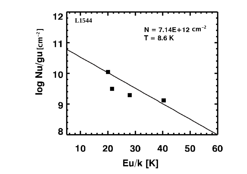
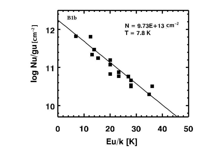
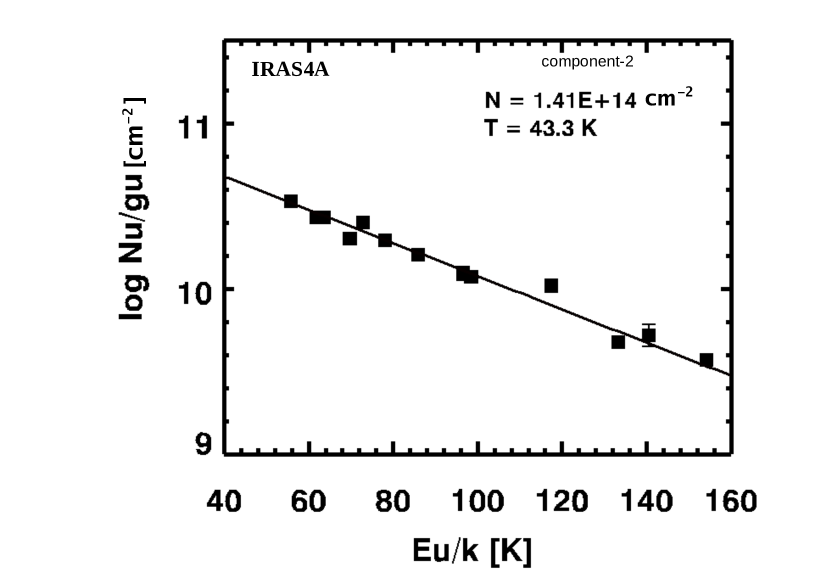
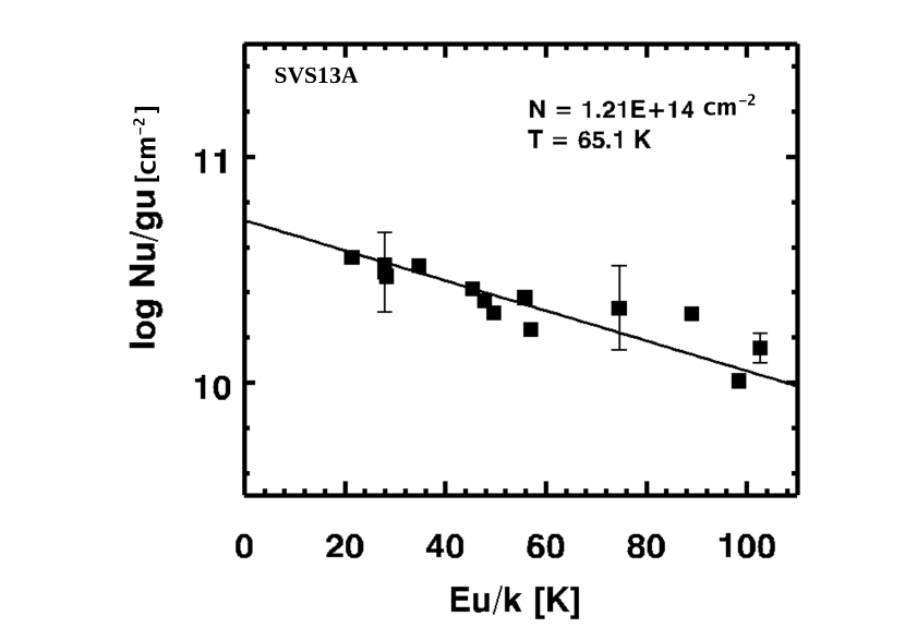
Figure 7: Rotational diagram for CH₃OH obtained with various sources. The black points are the position of the data points, the vertical bars are the error bars estimated, and the red lines are the fitted lines to the rotational diagram. The obtained column densities and the excitation temperatures along with the error bars are mentioned in the top right corner of each box.

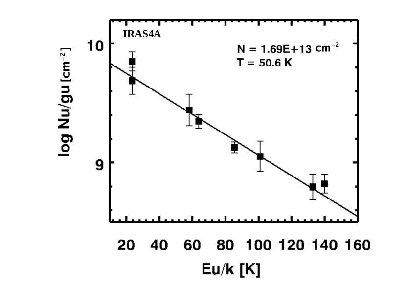
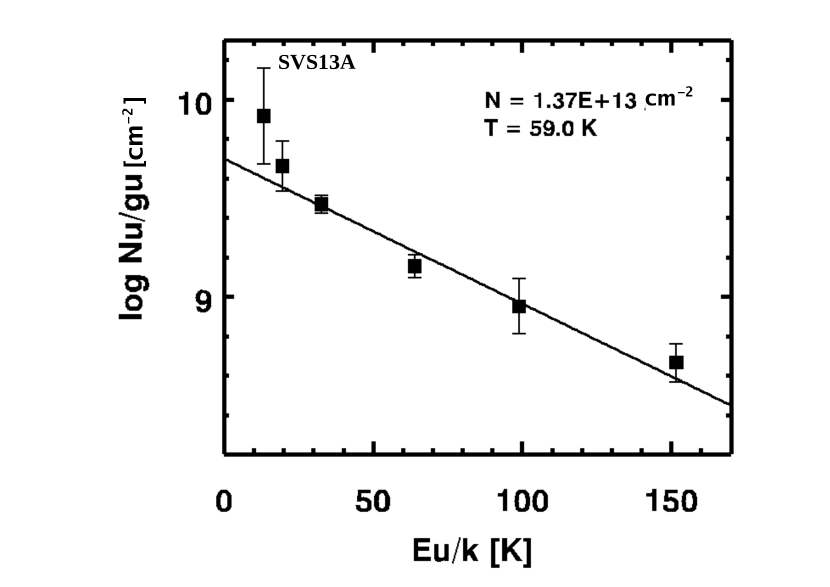
Figure 10: Rotational diagram for C₂H₅OH obtained for various sources. Here, we consider the source size and beam size are same. The symbols represent the same as those depicted in Figure 7.

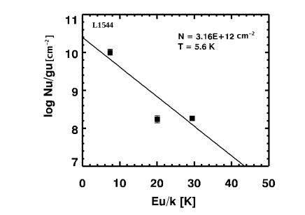
Figure 11: Rotational diagram for HCCCHO obtained for one source. Here, we consider the source size and beam size are same. The symbols represent the same as those depicted in Figure 7.

Figure 12: Rotational diagram for CH₃OCH₃, v = 0 obtained towards IRAS4A. The symbols represent the same as those depicted in Figure 7.

Appendix D Monte Carlo Markov chain method

The Markov Chain Monte Carlo (MCMC) is one of the most important and popular concept in Bayesian Statistics. Understanding the physical conditions in star-forming regions is a challenge nowadays as the chemistry in the star-forming regions are complicated and varies non-linearly with time and other physical conditions. In astrochemistry we use many trial and error grid-based analysis using simple statistics. But when the parameter space are large, heterogeneous and complex this approach fails. To interpret the astrochemical conditions a new method using Bayesian approach MCMC is implemented by an iterative process to solve it using simulation. The MCMC method is an interactive process that goes through all line parameters (e.g., molecular column density, excitation temperature, source size, line width) with a random walk and heads into the solution’s space and the final solution is obtained by $\chi^{2}$ minimization. As well as rotational diagram method MCMC can also be used to obtain the best suitable physical conditions only for those species for which multiple or at-least more than two transitions are observed with different upstate energies. The $\chi^{2}$ is defined as,

$${\rm{\chi_{i}}^{2}=\sum_{j=1}^{N_{i}}\frac{(I_{obs,ij}-I_{model,ij})^{2}}{rms^{2}_{i}+(cal_{i}\times I_{obs,ij})^{2}}},$$ (D1)

where, ${\rm I_{obs,ij}}$ and ${\rm I_{model,ij}}$ are observed and modeled intensity in the channel j of transition i respectively, rms_i is the RMS of the spectrum i, and cal_i is the calibration error. Here, the MCMC method is only used to fit the observed transitions of those species for which multiple transitions are observed. Here we employed the MCMC method from the CASSIS scripting interface to fit the observed lines of those seven COMs ($\rm{CH_{3}OH,CH_{3}CHO,CH_{3}OCHO,C_{2}H_{5}OH,HCCCHO,CH_{3}OCH_{3},CH_{3}CN}$), which we have considered towards different star-forming regions. Since we obtained a beam average column density with the rotational diagram analysis, we ignored the beam filling factor for the MCMC calculation. In some cases (CH₃OH iand CH₃CHO in IRAS4A), we employ a two-component MCMC fitting to have a better match with the observation. The components are considered based on their temperature. Details are described in section 3. We also kept the LSR velocity constant at 7.2, 6.5, 7.2, 2.6, and 8.4 km/s, respectively, for L1544, B1-b, IRAS4A, L1157-mm, and SVS13A. For the fitting, we varied FWHM, column density, and excitation temperature (T_ex) and obtained the best fit parameters from the LTE fitting using MCMC method. All the parameters along with the best fitted values of the physical parameters are noted in Table 1. Spectral fit for all the transitions arose from various molecules are shown in Figure 1, 2, 3, 4, 5, 6, 7, 8, and 9.

Table 1: Summary of the best fitted line parameters obtained by using MCMC method.

Species	Source	Frequency	FWHM range	Best fitted	Column density	Best fitted column	Tex range	Best fitted	Best fitted	Optical depth
		(GHz)	used (km.s-1)	FWHM (Km.s-1)	range used (cm-2)	density (cm-2)	used (K)	Tex (K)	VLSR (km.s-1)	($\tau$)
CH3OH	L1544	84.5211								$1.98\times 10^{-3}$
		96.7445	0.3-0.5	0.39$\pm$0.03	$1.0\times 10^{11}-1.0\times 10^{14}$	(4.60$\pm$0.92)$\times 10^{12}$	3.5-17.0	12.9$\pm$3.07	7.2	$5.86\times 10^{-3}$
		96.7555								$2.44\times 10^{-3}$
		97.5828								$3.97\times 10^{-3}$
	B1-b	96.7393								$2.08\times 10^{-1}$
		96.7413								$5.98\times 10^{-1}$
		96.7445	1.0-3.0	1.50$\pm$0.10	$1.0\times 10^{13}-1.0\times 10^{15}$	$(1.60\pm 0.12)\times 10^{14}$	5.0-25.0	7.27$\pm$0.86	6.5	$9.83\times 10^{-2}$
		96.7555								$2.55\times 10^{-2}$
		108.8939								$1.83\times 10^{-1}$
		145.0937								$5.11\times 10^{-2}$
		145.1031								$2.18\times 10^{-1}$
		157.2708								$1.25\times 10^{-1}$
		157.2760	1.0-3.0	1.05$\pm$0.08	$1.0\times 10^{13}-1.0\times 10^{15}$	$(5.90\pm 0.51)\times 10^{13}$	5.0-25.0	9.06$\pm$1.26	6.5	$1.23\times 10^{-1}$
		165.0501								$5.15\times 10^{-2}$
		165.0611								$5.13\times 10^{-2}$
		165.0992								$3.31\times 10^{-2}$
		170.0605								$3.04\times 10^{-2}$
		213.4270								$1.47\times 10^{-1}$
		254.0153	1.0-3.0	1.0$\pm$0.09	$1.0\times 10^{13}-1.0\times 10^{15}$	$(1.20\pm 0.32)\times 10^{14}$	5.0-25.0	6.77$\pm$0.95	6.5	$1.89\times 10^{-1}$
		261.8056								$1.68\times 10^{-1}$
	IRAS4A	96.7555								$1.14\times 10^{-2}$/$2.62\times 10^{-3}$
		108.8939								$1.52\times 10^{-1}$/$3.57\times 10^{-3}$
		143.8657								$3.50\times 10^{-2}$/$6.90\times 10^{-3}$
		155.3208								$2.89\times 10^{-10}$/$1.07\times 10^{-3}$
		155.9975								$1.73\times 10^{-8}$/$1.99\times 10^{-3}$
		156.4889								$6.71\times 10^{-7}$/$3.41\times 10^{-3}$
		156.8285								$1.69\times 10^{-5}$/$5.36\times 10^{-3}$
		157.0486								$2.75\times 10^{-4}$/$7.70\times 10^{-3}$
		157.1789								$2.88\times 10^{-3}$/$1.00\times 10^{-2}$
		165.0501				$Component1$				$6.79\times 10^{-2}$/$5.78\times 10^{-3}$
		165.0611	1.0-3.5	3.03$\pm$0.27	$1.0\times 10^{13}-1.0\times 10^{15}$	$(1.80\pm 0.29)\times 10^{14}$	5.0-30.0	5.62$\pm$1.68	7.2	$4.94\times 10^{-2}$/$8.42\times 10^{-3}$
		165.0992								$1.99\times 10^{-2}$/$9.62\times 10^{-3}$
		165.6786				$Component2$				$7.34\times 10^{-5}$/$6.48\times 10^{-3}$
		166.1690	1.0-3.5	3.50$\pm$0.47	$1.0\times 10^{13}-1.0\times 10^{15}$	$(2.00\pm 0.28)\times 10^{14}$	30.0-70.0	35.14$\pm$3.86	7.2	$4.65\times 10^{-6}$/$4.66\times 10^{-3}$
		213.4270								$7.56\times 10^{-2}$/$5.13\times 10^{-3}$
		230.0270								$3.92\times 10^{-3}$/$2.88\times 10^{-3}$
		241.8790								$1.37\times 10^{-3}$/$1.05\times 10^{-2}$
		251.7384								$9.90\times 10^{-7}$/$4.28\times 10^{-3}$
		251.8665								$5.29\times 10^{-5}$/$5.01\times 10^{-3}$
		251.9170								$1.54\times 10^{-4}$/$3.63\times 10^{-3}$
		251.9848								$4.59\times 10^{-9}$/$2.33\times 10^{-3}$
		252.0904								$1.36\times 10^{-10}$/$1.49\times 10^{-3}$
		254.0153								$1.13\times 10^{-1}$/$3.85\times 10^{-3}$
		261.8056								$7.95\times 10^{-2}$/$8.53\times 10^{-3}$
	SVS13A	85.5681								$3.08\times 10^{-4}$
		96.7555	2.0-4.5	4.04$\pm$0.59	$1.0\times 10^{13}-1.0\times 10^{15}$	$(3.00\pm 2.42)\times 10^{14}$	40.0-200.0	96.72$\pm$18.77	8.6	$3.51\times 10^{-4}$
		111.2894								$3.65\times 10^{-4}$
		143.8657								$1.01\times 10^{-3}$
		156.6023	2.0-3.5	3.47$\pm$0.39	$1.0\times 10^{13}-1.0\times 10^{15}$	$(2.80\pm 0.62)\times 10^{14}$	40.0-100.0	96.70$\pm$14.03	8.6	$1.09\times 10^{-3}$
		218.4400								$2.37\times 10^{-3}$
		229.7587								$1.93\times 10^{-3}$
		241.7001								$2.97\times 10^{-3}$
		241.7913								$3.60\times 10^{-3}$
		241.8790	2.0-3.5	3.36$\pm$0.24	$1.0\times 10^{13}-1.0\times 10^{15}$	$(1.50\pm 0.17)\times 10^{14}$	40.0-100.0	68.69$\pm$8.41	8.6	$2.61\times 10^{-3}$
		243.9157								$2.81\times 10^{-3}$
		251.7384								$1.92\times 10^{-3}$
		261.8056								$1.43\times 10^{-3}$
		266.8381								$2.76\times 10^{-3}$

Species	Source	Frequency	FWHM range	Best fitted	Column density	Best fitted column	Tex range	Best fitted	Best fitted	Optical depth
		(GHz)	used (km.s-1)	FWHM (Km.s-1)	range used (cm-2)	density (cm-2)	used (K)	Tex (K)	VLSR (km.s-1)	($\tau$)
CH3CHO	L1544	93.5809								$1.32\times 10^{-2}$
		93.5952								$1.31\times 10^{-2}$
		95.9474	0.3-0.6	0.39$\pm$0.09	$1.0\times 10^{11}-1.0\times 10^{13}$	$(6.10\pm 3.55)\times 10^{11}$	3.5-20.0	6.04$\pm$4.42	7.2	$1.93\times 10^{-2}$
		95.9634								$1.96\times 10^{-2}$
		98.8633								$1.25\times 10^{-2}$
		98.9009								$1.26\times 10^{-1}$
	B1-b	93.5809								$1.65\times 10^{-2}$
		93.5952								$1.64\times 10^{-2}$
		95.9634								$2.30\times 10^{-2}$
		96.4256	0.5-2.0	1.49$\pm$0.36	$1.0\times 10^{11}-5.0\times 10^{13}$	$(4.70\pm 2.39)\times 10^{12}$	6.0-100.0	7.52$\pm$6.61	6.5	$5.78\times 10^{-3}$
		96.4755								$5.70\times 10^{-3}$
		98.8633								$1.59\times 10^{-2}$
		98.9009								$1.61\times 10^{-2}$
		138.2849	0.5-1.5	1.38$\pm$0.24	$1.0\times 10^{11}-5.0\times 10^{13}$	$(4.10\pm 2.84)\times 10^{12}$	6.0-100.0	10.81$\pm$3.63	6.5	$5.08\times 10^{-3}$
		138.3196								$5.11\times 10^{-3}$
		152.6352								$4.59\times 10^{-3}$
		155.1796								$1.81\times 10^{-3}$
	IRAS4A	74.8917								$8.67\times 10^{-3}$/$1.89\times 10^{-4}$
		74.9241								$8.60\times 10^{-3}$/$1.88\times 10^{-4}$
		76.8789								$1.14\times 10^{-2}$/$2.13\times 10^{-4}$
		77.0386								$3.79\times 10^{-3}$/$1.41\times 10^{-4}$
		77.2183								$3.80\times 10^{-3}$/$1.41\times 10^{-4}$
		79.0993								$8.75\times 10^{-3}$/$1.98\times 10^{-4}$
		93.5809								$9.64\times 10^{-3}$/$2.85\times 10^{-4}$
		93.5952								$9.58\times 10^{-3}$/$2.85\times 10^{-4}$
		95.9474								$1.22\times 10^{-2}$/$3.13\times 10^{-4}$
		96.2742								$4.56\times 10^{-3}$/$2.32\times 10^{-4}$
		96.4256								$4.56\times 10^{-3}$/$2.31\times 10^{-4}$
		96.4755								$4.51\times 10^{-3}$/$2.31\times 10^{-4}$
		98.8633								$9.56\times 10^{-3}$/$2.98\times 10^{-4}$
		112.248								$9.02\times 10^{-3}$/$3.88\times 10^{-4}$
		112.2545								$8.97\times 10^{-3}$/$3.87\times 10^{-4}$
		133.8305								$8.85\times 10^{-3}$/$5.22\times 10^{-4}$
		138.2849								$6.88\times 10^{-3}$/$5.08\times 10^{-4}$
		138.3196				Component 1				$6.92\times 10^{-3}$/$5.08\times 10^{-4}$
		152.6352	2.0-3.5	3.30$\pm$0.22	$1.0\times 10^{12}-1.0\times 10^{14}$	$(1.30\pm 0.21)\times 10^{13}$	8.0-30.0	11.07$\pm$3.48	7.2	$6.27\times 10^{-3}$/$6.18\times 10^{-4}$
		155.3421				Component 2				$2.58\times 10^{-3}$/$5.19\times 10^{-4}$
		168.0934	2.0-3.5	2.3$\pm$0.32	$1.0\times 10^{12}-1.0\times 10^{14}$	$(1.10\pm 0.21)\times 10^{13}$	30.0-80.0	71.2$\pm$5.17	7.2	$3.36\times 10^{-3}$/$6.66\times 10^{-4}$
		208.2285								$1.13\times 10^{-3}$/$8.04\times 10^{-4}$
		211.2738								$4.75\times 10^{-4}$/$6.92\times 10^{-4}$
		212.2571								$1.63\times 10^{-4}$/$5.68\times 10^{-4}$
		214.8450								$4.63\times 10^{-4}$/$7.00\times 10^{-4}$
		216.6302								$8.10\times 10^{-4}$/$7.85\times 10^{-4}$
		223.6601								$4.77\times 10^{-4}$/$7.99\times 10^{-4}$
		242.1060								$2.04\times 10^{-4}$/$8.02\times 10^{-4}$
		250.8291								$7.31\times 10^{-6}$/$4.55\times 10^{-4}$
		250.9345								$3.16\times 10^{-5}$/$5.94\times 10^{-4}$
		251.4893								$3.16\times 10^{-5}$/$5.95\times 10^{-4}$
		254.8271								$8.67\times 10^{-5}$/$7.22\times 10^{-4}$
		255.3269								$1.47\times 10^{-4}$/$7.97\times 10^{-4}$
		262.9601								$8.63\times 10^{-5}$/$8.02\times 10^{-4}$
		205.1707								$9.80\times 10^{-4}$
	SVS13A	211.2430								$8.18\times 10^{-4}$
		211.2738								$8.17\times 10^{-4}$
		216.5819	0.5-2.5	2.45$\pm$0.33	$1.0\times 10^{12}-1.0\times 10^{14}$	$(7.20\pm 4.89)\times 10^{12}$	30.0-200.0	45.16$\pm$11.4	8.6	$9.66\times 10^{-4}$
		230.3019								$7.74\times 10^{-4}$
		242.1060								$8.51\times 10^{-4}$
		251.4893								$5.34\times 10^{-4}$

Species	Source	Frequency	FWHM range	Best fitted	Column density	Best fitted column	Tex range	Best fitted	Best fitted	Optical depth
		(GHz)	used (km.s-1)	FWHM (Km.s-1)	range used (cm-2)	density (cm-2)	used (K)	Tex (K)	VLSR (km.s-1)	($\tau$)
CH3OCHO	B1-b	88.8516								$1.48\times 10^{-3}$
		90.1457								$1.30\times 10^{-3}$
		90.1564	1.0-2.0	1.64$\pm$0.21	$1.0\times 10^{11}-1.0\times 10^{14}$	$(1.20\pm 1.00)\times 10^{13}$	15.0-100.0	18.52$\pm$22.81	6.5	$1.30\times 10^{-3}$
		100.2946								$1.03\times 10^{-3}$
		100.4822								$1.49\times 10^{-3}$
		103.4786								$1.35\times 10^{-3}$
	IRAS4A	129.2963∗								$3.92\times 10^{-4}$
		132.9287								$4.24\times 10^{-4}$
		135.9219								$2.90\times 10^{-4}$
		141.0443	1.0-3.0	1.86$\pm$0.54	$1.0\times 10^{12}-1.0\times 10^{14}$	$(3.90\pm 1.54)\times 10^{13}$	30.0-130.0	73.87$\pm$24.37	7.2	$4.45\times 10^{-4}$
		158.6937								$4.53\times 10^{-4}$
		158.7043								$4.53\times 10^{-4}$
		200.9563								$4.21\times 10^{-4}$
		206.6194								$5.13\times 10^{-4}$
		216.2165								$5.06\times 10^{-4}$
		228.6288	1.0-3.0	1.35$\pm$0.50	$1.0\times 10^{12}-1.0\times 10^{14}$	$(3.40\pm 1.72)\times 10^{13}$	30.0-130.0	81.32$\pm$18.46	7.2	$4.28\times 10^{-4}$
		240.0211								$4.75\times 10^{-4}$
		247.0441								$4.38\times 10^{-4}$
		249.5781								$3.57\times 10^{-4}$
	SVS13A	100.4906	1.0-3.0	1.95$\pm$0.53	$1.0\times 10^{12}-1.0\times 10^{15}$	$(6.40\pm 5.17)\times 10^{13}$	40.0-200.0	86.94$\pm$33.36	8.6	$3.04\times 10^{-4}$
		164.2059								$4.73\times 10^{-4}$
		210.4632								$2.81\times 10^{-4}$
		218.2809	1.0-3.0	2.10$\pm$0.37	$1.0\times 10^{12}-1.0\times 10^{15}$	$(7.80\pm 1.88)\times 10^{13}$	40.0-200.0	113.84$\pm$23.41	8.6	$4.15\times 10^{-4}$
		222.4214								$2.55\times 10^{-4}$
		269.0780								$4.06\times 10^{-4}$
$\rm{C_{2}H_{5}OH}$	IRAS4A	129.6657								$2.84\times 10^{-4}$
		133.3234	0.4-1.5	1.46$\pm$0.26	$1.0\times 10^{12}-1.0\times 10^{14}$	$(2.60\pm 1.61)\times 10^{13}$	30.0-100.0	60.14$\pm$16.62	7.2	$5.90\times 10^{-4}$
		148.3040								$2.76\times 10^{-4}$
		159.4140								$2.92\times 10^{-4}$
		205.4584								$5.22\times 10^{-4}$
		209.8652	0.4 - 0.8	0.74$\pm$0.06	$1.0\times 10^{12}-1.0\times 10^{14}$	$(1.60\pm 0.59)\times 10^{13}$	30.0 - 100.0	88.46$\pm$18.28	7.2	$2.29\times 10^{-4}$
		227.8919								$2.72\times 10^{-4}$
		230.9913								$5.63\times 10^{-4}$
	SVS13A	84.5958								$4.02\times 10^{-4}$
		130.2463	0.5 - 2.0	0.92$\pm$0.41	$1.0\times 10^{12}-1.0\times 10^{14}$	$(1.70\pm 1.59)\times 10^{13}$	10.0-100.0	45.63$\pm$17.28	8.6	$4.64\times 10^{-4}$
		153.4842								$5.24\times 10^{-4}$
		205.4584								$8.26\times 10^{-4}$
		244.6339	0.5-2.0	0.97$\pm$0.28	$1.0\times 10^{12}-1.0\times 10^{14}$	$(1.50\pm 0.86)\times 10^{13}$	10.0-100.0	59.58$\pm$21.85	8.6	$2.78\times 10^{-4}$
		270.4441								$7.21\times 10^{-4}$
$\rm{HCCCHO}$	L1544	83.7758								$1.43\times 10^{-3}$
		99.0391	0.3-0.6	0.43$\pm$0.07	$1.0\times 10^{11}-1.0\times 10^{13}$	$(4.00\pm 1.33)\times 10^{11}$	3.5-20.0	17.40$\pm$5.24	7.2	$6.28\times 10^{-5}$
		102.2980								$1.28\times 10^{-3}$
$\rm{CH_{3}OCH_{3}}$	L1544	99.324362								$3.66\times 10^{-4}$
		99.324364	0.1-1.0	$0.41\pm$0.22	$1.0\times 10^{11}-1.0\times 10^{13}$	$(2.20\pm 1.61)\times 10^{12}$	3.5-20.0	$15.47\pm 2.71$	7.2	$5.49\times 10^{-4}$
		99.325217								$1.46\times 10^{-3}$
		99.326072								$9.15\times 10^{-4}$
	B1-b	99.324362								$1.49\times 10^{-3}$
		99.324364	0.5-1.0	$0.9\pm 0.12$	$6.0\times 10^{11}-6.0\times 10^{13}$	$(8.50\pm 5.52)\times 10^{12}$	5.0-25.0	$9.85\pm 4.56$	6.5	$2.23\times 10^{-3}$
		99.325217								$5.95\times 10^{-3}$
		99.326072								$3.72\times 10^{-3}$
	IRAS4A	162.5295								$5.38\times 10^{-4}$
		209.5156								$6.02\times 10^{-4}$
		225.5991	1.0-3.0	2.11$\pm$0.35	$1.0\times 10^{12}-1.0\times 10^{14}$	$(2.10\pm 1.03)\times 10^{13}$	30.0-130.0	45.28$\pm$28.29	7.2	$5.83\times 10^{-4}$
		241.9465								$5.45\times 10^{-4}$
$\rm{CH_{3}CN}$	IRAS4A	73.588799								$1.97\times 10^{-3}$
		73.590218								$2.96\times 10^{-3}$
		91.979994								$8.26\times 10^{-4}$
		91.985314								$2.61\times 10^{-3}$
		91.987087								$3.83\times 10^{-3}$
		110.364353								$3.08\times 10^{-4}$
		110.381372								$3.03\times 10^{-3}$
		110.383499								$4.38\times 10^{-3}$
		128.757030								$3.48\times 10^{-4}$
		128.769436								$1.07\times 10^{-3}$
		128.776881				component1				$3.16\times 10^{-3}$
		128.779363	1.5-3.0	$2.9\pm 0.19$	$1.0\times 10^{11}-1.0\times 10^{13}$	$(9.9\pm 3.15)\times 10^{11}$	20.0-50.0	$21.02\pm 3.24$	7.2	$4.54\times 10^{-3}$
		147.163244				component2				$1.04\times 10^{-3}$
		147.171751	1.5-3.0	$2.9\pm 0.12$	$1.0\times 10^{11}-1.0\times 10^{13}$	$(1.7\pm 0.38)\times 10^{12}$	50.0-80.0	$70.11\pm 5.32$	7.2	$3.04\times 10^{-3}$
		147.174588								$4.34\times 10^{-3}$
		165.540377								$3.21\times 10^{-4}$
		165.556321								$9.38\times 10^{-4}$
		165.565891								$2.70\times 10^{-3}$
		165.569081								$3.84\times 10^{-3}$
		202.320442								$2.16\times 10^{-4}$
		220.709016								$1.61\times 10^{-4}$

Species	Source	Frequency	FWHM range	Best fitted	Column density	Best fitted column	Tex range	Best fitted	Best fitted	Optical depth
		(GHz)	used (km.s-1)	FWHM (Km.s-1)	range used (cm-2)	density (cm-2)	used (K)	Tex (K)	VLSR (km.s-1)	($\tau$)
	SVS13A	91.979994								$2.705\times 10^{-4}$
		91.985314								$3.996\times 10^{-4}$
		91.987087								$4.535\times 10^{-4}$
		110.364353								$4.281\times 10^{-4}$
		110.374989								$3.890\times 10^{-4}$
		110.381372								$5.499\times 10^{-4}$
		110.383499								$6.162\times 10^{-4}$
		128.776881	1.5-3.5	$3.48\pm 0.09$	$5.0\times 10^{11}-5.0\times 10^{13}$	$(2.8\pm 0.57)\times 10^{12}$	40.0-200.0	$83.55\pm 19.34$	8.6	$7.041\times 10^{-4}$
		128.779363								$7.832\times 10^{-4}$
		147.171751								$8.538\times 10^{-4}$
		165.565891								$9.913\times 10^{-4}$
		220.709016								$1.210\times 10^{-3}$
		220.730260								$9.624\times 10^{-4}$
		220.743010								$1.270\times 10^{-3}$
		220.747261								$1.394\times 10^{-3}$
		239.119504								$9.939\times 10^{-4}$
		257.527383								$1.441\times 10^{-3}$

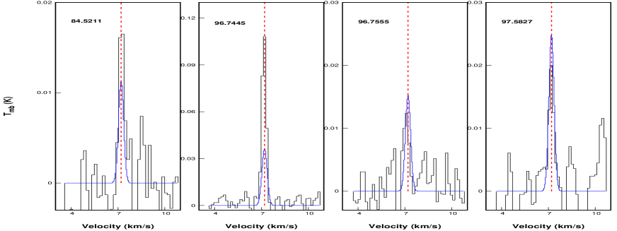
Figure 1: MCMC fitting of the observed transitions of $\rm{CH_{3}OH}$ in L1544. Black lines represent the observed spectra, and blue represents the modeled spectral profile. The vertical red dashed line represents the V_lsr

.

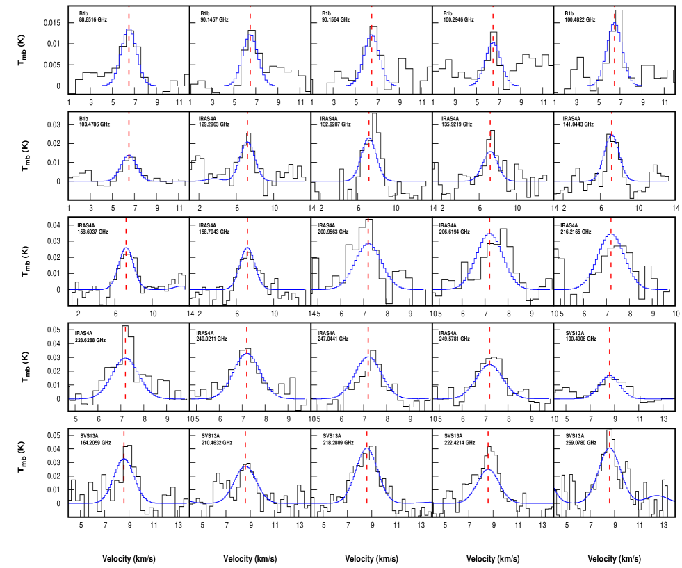
Figure 6: Same as Figure 1 for $\rm{CH_{3}OCHO}$.

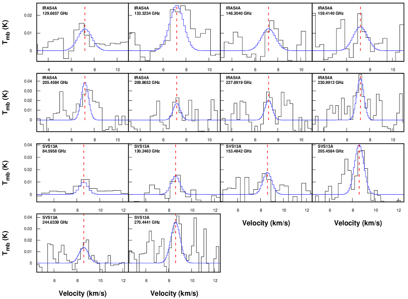
Figure 7: Same as Figure 1 for $\rm{C_{2}H_{5}OH}$.

Figure 10: Same as Figure 1 for $\rm{CH_{3}CN}$ in IRAS4A.

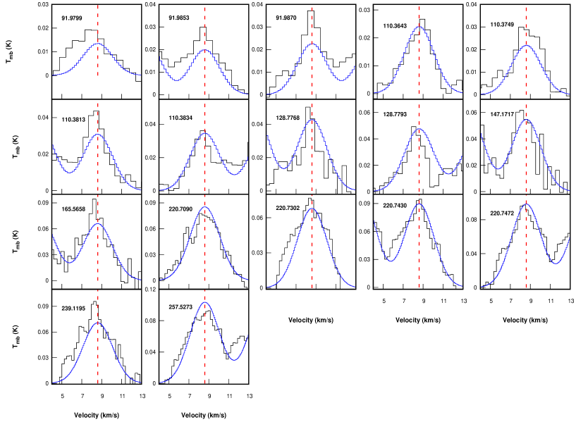
Figure 11: Same as Figure 1 for $\rm{CH_{3}CN}$ in SVS13A.

Appendix E Beam dilution effect

The present data have a large frequency width, and the beam size changes significantly. Therefore, we need to assume the size of the emitting region for the COMs and apply the appropriate beam dilution factor for each source to see its effect. Figure 1 shows the abundances (obtained from the rotational diagram analysis) at the different evolutionary stages of low-mass star-forming regions by considering the beam dilution effect. Additionally, we note the obtained abundances in Table 1. The obtained intensities in the rotational diagram analysis are scaled by considering the beam dilution factor for each source. For simplicity, we consider an average source size, and the choice of source size for each source is justified below:
L1544: Caselli et al. (2019, 2022) obtained a compact component of $\sim$ 10$\arcsec$ in L1544. Assuming the emission of the COMs from this region, we consider a source size of 10$\arcsec$ (see Figure 1 and in Table 1).
B1-b: Marcelino et al. (2018a) employed a source model with two components; an inner hot and compact component (200 K, 0.35$\arcsec$) and an outer and colder component (60 K, 0.6$\arcsec$) to fit the observed line profiles in B1b-S. Additionally, they considered another component mimicking the envelope at $\sim 10$ K. In our analysis, we obtain a rotational temperature $\sim$ $10$ K for all molecules in this source, we consider a source size of 10$\arcsec$, which is comparable to the smallest beam size in this data (see Figure 1).
IRAS16293-2422: We consider the abundances obtained directly from the ALMA Protostellar interferometric line survey (PILS) (for details, see Section 3.4.1).
IRAS4A: López-Sepulcre et al. (2015) considered a source size of 0.5$\arcsec$ to perform the RD analysis for NH₂CHO and HNCO in IRAS4A. We adopt similar source size of $0.5{\arcsec}$ to consider beam dilution effect ( see Table 1 and Figure 1).
SVS13A: López-Sepulcre et al. (2015) considered a source size of 1.0$\arcsec$ to perform the RD analysis for NH₂CHO and HNCO in SVS13A and Bianchi et al. (2019) considered a source size of 0.3$\arcsec$ for various iCOMs . We adopt both sizes to consider the beam dilution effect ( see Table 1 and Figure 1).

Figure 1 depicts that even with the beam dilution effect, the obtained trend is similar (the abundance is gradually increasing up to class 0 and then decreased) to that obtained without the beam dilution effect shown in Figure 1. A very similar trend was also obtained when we used the abundances from various interferometric observations in Figure 6.

Table 1: Column density and abundance of the observed species considering the beam dilution factor.

Source	Size	N(H2)	Species	Column density	Abundance
			CH3OH	$5.0\times 10^{13}$	$7.4\times 10^{-11}$
			CH3CHO	$1.1\times 10^{13}$	$1.6\times 10^{-11}$
L1544	10$\arcsec$	$6.8\times 10^{23c}$	CH3OCHO	$3.7\times 10^{13*}$	$5.4\times 10^{-11}$
			C2H5OH	$\cdots$	$\cdots$
			HCCCHO	$2.1\times 10^{13}$	$3.1\times 10^{-11}$
			CH3OCH3	$1.7\times 10^{13**}$	$2.5\times 10^{-11}$
			CH3CN	$4.85\times 10^{12**}$	$7.1\times 10^{-12}$
			CH3OH	$6.2\times 10^{14}$	$7.8\times 10^{-10}$
			CH3CHO	$5.1\times 10^{13}$	$6.4\times 10^{-11}$
B1-b	10$\arcsec$	$7.9\times 10^{23d}$	CH3OCHO	$5.4\times 10^{13}$	$6.8\times 10^{-11}$
			C2H5OH	$1.0\times 10^{14*}$	$1.2\times 10^{-10}$
			HCCCHO	$2.6\times 10^{13*}$	$3.2\times 10^{-11}$
			CH3OCH3	$6.0\times 10^{13**}$	$7.6\times 10^{-11}$
			CH3CN	$4.95\times 10^{12**}$	$6.3\times 10^{-12}$
			CH3OH (hot)	$9.7\times 10^{16}$	$3.9\times 10^{-8}$
			CH3CHO	$4.4\times 10^{15}$	$1.8\times 10^{-9}$
IRAS4A	0.5$\arcsec$	$2.5\times 10^{24}$	CH3OCHO	$2.4\times 10^{16}$	$9.5\times 10^{-9}$
	López-Sepulcre et al. (2015)	López-Sepulcre et al. (2015)	C2H5OH	$1.3\times 10^{16}$	$5.2\times 10^{-9}$
			HCCCHO	$4.9\times 10^{15*}$	$2.0\times 10^{-9}$
			CH3OCH3	$6.7\times 10^{15}$	$2.7\times 10^{-9}$
			CH3CN	$3.55\times 10^{15}$	$1.4\times 10^{-09}$
			CH3OH	$3.7\times 10^{16}$	$3.7\times 10^{-9}$
			CH3CHO	$8.6\times 10^{14}$	$8.6\times 10^{-11}$
SVS13A	1$\arcsec$	$1.0\times 10^{25}$	CH3OCHO	$9.7\times 10^{15}$	$9.7\times 10^{-10}$
	López-Sepulcre et al. (2015)	López-Sepulcre et al. (2015)	C2H5OH	$2.8\times 10^{15}$	$2.8\times 10^{-10}$
			HCCCHO	$3.9\times 10^{16*}$	$3.9\times 10^{-9}$
			CH3OCH3	$1.3\times 10^{16a}$	$1.3\times 10^{-9}$
			CH3CN	$5.16\times 10^{14}$	$5.2\times 10^{-11}$
			CH3OH	$4.1\times 10^{17}$	$1.4\times 10^{-7}$
			CH3CHO	$9.6\times 10^{15}$	$3.2\times 10^{-9}$
SVS13A	0.3$\arcsec$	$3.0\times 10^{24}$	CH3OCHO	$1.1\times 10^{17}$	$3.6\times 10^{-8}$
	Bianchi et al. (2019)	Chen et al. (2009)	C2H5OH	$3.1\times 10^{16}$	$1.0\times 10^{-8}$
			HCCCHO	$4.3\times 10^{17*}$	$1.4\times 10^{-7}$
			CH3OCH3	$1.4\times 10^{17b}$	$4.7\times 10^{-8}$
			CH3CN	$5.74\times 10^{15}$	$1.9\times 10^{-09}$

Note: ^∗ indicates upper limit, ^∗∗ indicates LTE derived value, ^a is scaled value from Bianchi et al. (2019), and ^b from Bianchi et al. (2019)., ^c taken from Hily-Blant et al. (2022) after scaling it for 10$\arcsec$, ^d taken from Daniel et al. (2013) after scaling it for 10$\arcsec$.

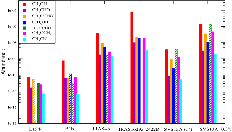
Figure 1: Abundances of the COMs at the different evolutionary stages of low-mass star-forming regions.

References

- Andre et al. (1993) Andre, P., Ward-Thompson, D., & Barsony, M. 1993, ApJ, 406, 122
- Anglada et al. (2000) Anglada, G., Rodríguez, L. F., & Torrelles, J. M. 2000, ApJ, 542, L123
- Bachiller et al. (1998) Bachiller, R., Guilloteau, S., Gueth, F., et al. 1998, A&A, 339, L49
- Balucani et al. (2015) Balucani, N., Ceccarelli, C., & Taquet, V. 2015, Monthly Notices of the Royal Astronomical Society: Letters, 449, L16
- Belloche et al. (2020) Belloche, A., Maury, A. J., Maret, S., et al. 2020, A&A, 635, A198
- Bhat et al. (2022) Bhat, B., Gorai, P., Mondal, S. K., Chakrabarti, S. K., & Das, A. 2022, Advances in Space Research, 69, 415
- Bianchi et al. (2022a) Bianchi, E., López-Sepulcre, A., Ceccarelli, C., et al. 2022a, ApJ, 928, L3
- Bianchi et al. (2019) Bianchi, E., Codella, C., Ceccarelli, C., et al. 2019, MNRAS, 483, 1850
- Bianchi et al. (2022b) Bianchi, E., Ceccarelli, C., Codella, C., et al. 2022b, A&A, 662, A103
- Bizzocchi et al. (2014) Bizzocchi, L., Caselli, P., Spezzano, S., & Leonardo, E. 2014, A&A, 569, A27
- Blake et al. (1995) Blake, G. A., Sandell, G., van Dishoeck, E. F., et al. 1995, ApJ, 441, 689
- Blake et al. (1987) Blake, G. A., Sutton, E., Masson, C., & Phillips, T. 1987, Astrophysical Journal, 315, 621
- Bockelée-Morvan et al. (2000) Bockelée-Morvan, D., Lis, D. C., Wink, J. E., et al. 2000, A&A, 353, 1101
- Bottinelli et al. (2007) Bottinelli, S., Ceccarelli, C., Williams, J. P., & Lefloch, B. 2007, A&A, 463, 601
- Bottinelli et al. (2004) Bottinelli, S., Ceccarelli, C., Lefloch, B., et al. 2004, ApJ, 615, 354
- Calcutt et al. (2018) Calcutt, H., Jørgensen, J. K., Müller, H. S. P., et al. 2018, A&A, 616, A90
- Caselli & Ceccarelli (2012) Caselli, P., & Ceccarelli, C. 2012, A&A Rev., 20, 56
- Caselli et al. (1999) Caselli, P., Walmsley, C. M., Tafalla, M., Dore, L., & Myers, P. C. 1999, ApJ, 523, L165
- Caselli et al. (2002) Caselli, P., Walmsley, C. M., Zucconi, A., et al. 2002, ApJ, 565, 344
- Caselli et al. (2017) Caselli, P., Bizzocchi, L., Keto, E., et al. 2017, A&A, 603, L1
- Caselli et al. (2019) Caselli, P., Pineda, J. E., Zhao, B., et al. 2019, ApJ, 874, 89
- Caselli et al. (2022) Caselli, P., Pineda, J. E., Sipilä, O., et al. 2022, ApJ, 929, 13
- Cazaux et al. (2003) Cazaux, S., Tielens, A. G. G. M., Ceccarelli, C., et al. 2003, ApJ, 593, L51
- Cernicharo & Guelin (1987) Cernicharo, J., & Guelin, M. 1987, A&A, 176, 299
- Cernicharo et al. (2012) Cernicharo, J., Marcelino, N., Roueff, E., et al. 2012, ApJ, 759, L43
- Cernicharo et al. (2013) Cernicharo, J., Tercero, B., Fuente, A., et al. 2013, ApJ, 771, L10
- Chen et al. (2009) Chen, X., Launhardt, R., & Henning, T. 2009, The Astrophysical Journal, 691, 1729
- Choi et al. (2011) Choi, M., Kang, M., & Tatematsu, K. 2011, ApJ, 728, L34
- Choi et al. (1999) Choi, M., Panis, J.-F., & Evans, Neal J., I. 1999, ApJS, 122, 519
- Choi et al. (2010) Choi, M., Tatematsu, K., & Kang, M. 2010, ApJ, 723, L34
- Ciolek & Basu (2000) Ciolek, G. E., & Basu, S. 2000, ApJ, 529, 925
- Cuppen et al. (2017) Cuppen, H., Walsh, C., Lamberts, T., et al. 2017, Space Science Reviews, 212, 1
- Daniel et al. (2013) Daniel, F., Gérin, M., Roueff, E., et al. 2013, Astronomy & Astrophysics, 560, A3
- Das et al. (2008a) Das, A., Acharyya, K., Chakrabarti, S., & Chakrabarti, S. K. 2008a, A&A, 486, 209
- Das et al. (2010) Das, A., Acharyya, K., & Chakrabarti, S. K. 2010, MNRAS, 409, 789
- Das & Chakrabarti (2011) Das, A., & Chakrabarti, S. K. 2011, MNRAS, 418, 545
- Das et al. (2019) Das, A., Gorai, P., & Chakrabarti, S. K. 2019, A&A, 628, A73
- Das et al. (2016) Das, A., Sahu, D., Majumdar, L., & Chakrabarti, S. K. 2016, MNRAS, 455, 540
- Das et al. (2018) Das, A., Sil, M., Gorai, P., Chakrabarti, S. K., & Loison, J. C. 2018, ApJS, 237, 9
- De Simone et al. (2020a) De Simone, M., Ceccarelli, C., Codella, C., et al. 2020a, ApJ, 896, L3
- De Simone et al. (2020b) —. 2020b, ApJ, 896, L3
- Di Francesco et al. (2001) Di Francesco, J., Myers, P. C., Wilner, D. J., Ohashi, N., & Mardones, D. 2001, ApJ, 562, 770
- Diaz-Rodriguez et al. (2022) Diaz-Rodriguez, A. K., Anglada, G., Blázquez-Calero, G., et al. 2022, ApJ, 930, 91
- Doty et al. (2005) Doty, S. D., Everett, S. E., Shirley, Y. L., Evans, N. J., & Palotti, M. L. 2005, MNRAS, 359, 228
- Fuente et al. (2016) Fuente, A., Cernicharo, J., Roueff, E., et al. 2016, A&A, 593, A94
- Fuente et al. (2017) Fuente, A., Gerin, M., Pety, J., et al. 2017, A&A, 606, L3
- Galli et al. (2019) Galli, P. A. B., Loinard, L., Bouy, H., et al. 2019, A&A, 630, A137
- Garrod & Herbst (2006) Garrod, R. T., & Herbst, E. 2006, A&A, 457, 927
- Garrod et al. (2009) Garrod, R. T., Vasyunin, A. I., Semenov, D. A., Wiebe, D. S., & Henning, T. 2009, ApJ, 700, L43
- Garrod et al. (2007) Garrod, R. T., Wakelam, V., & Herbst, E. 2007, A&A, 467, 1103
- Gerin et al. (2009) Gerin, M., Marcelino, N., Biver, N., et al. 2009, Astronomy & Astrophysics, 498, L9
- Gerin et al. (2015) Gerin, M., Pety, J., Fuente, A., et al. 2015, A&A, 577, L2
- Ghosh et al. (2022) Ghosh, R., Sil, M., Kumar Mondal, S., et al. 2022, Research in Astronomy and Astrophysics, 22, 065021
- Goldsmith & Langer (1999) Goldsmith, P. F., & Langer, W. D. 1999, ApJ, 517, 209
- Gorai et al. (2020a) Gorai, P., Bhat, B., Sil, M., et al. 2020a, arXiv e-prints, arXiv:2003.09188
- Gorai et al. (2020b) Gorai, P., Das, A., Shimonishi, T., et al. 2020b, arXiv e-prints, arXiv:2011.02226
- Hasegawa et al. (1992) Hasegawa, T. I., Herbst, E., & Leung, C. M. 1992, ApJS, 82, 167
- Hily-Blant et al. (2022) Hily-Blant, P., Des Forêts, G. P., Faure, A., & Lique, F. 2022, Astronomy and Astrophysics-A&A, 658, A168
- Holdship et al. (2019) Holdship, J., Viti, S., Codella, C., et al. 2019, ApJ, 880, 138
- Huang & Hirano (2013) Huang, Y.-H., & Hirano, N. 2013, ApJ, 766, 131
- Hudson & Gerakines (2019) Hudson, R. L., & Gerakines, P. A. 2019, Monthly Notices of the Royal Astronomical Society, 482, 4009
- Irvine et al. (1988) Irvine, W. M., Brown, R., Cragg, D., et al. 1988, The Astrophysical Journal, 335, L89
- Jaber et al. (2014) Jaber, A. A., Ceccarelli, C., Kahane, C., & Caux, E. 2014, ApJ, 791, 29
- Jacobsen et al. (2019) Jacobsen, S. K., Jørgensen, J. K., Di Francesco, J., et al. 2019, A&A, 629, A29
- Jiménez-Serra et al. (2016) Jiménez-Serra, I., Vasyunin, A. I., Caselli, P., et al. 2016, ApJ, 830, L6
- Johnson et al. (2000) Johnson, D. G., Blitz, M. A., & Seakins, P. W. 2000, Physical Chemistry Chemical Physics (Incorporating Faraday Transactions), 2, 2549
- Johnstone et al. (2010) Johnstone, D., Rosolowsky, E., Tafalla, M., & Kirk, H. 2010, ApJ, 711, 655
- Jørgensen et al. (2004) Jørgensen, J. K., Hogerheijde, M. R., van Dishoeck, E. F., Blake, G. A., & Schöier, F. L. 2004, A&A, 413, 993
- Jørgensen et al. (2016) Jørgensen, J. K., van der Wiel, M. H. D., Coutens, A., et al. 2016, A&A, 595, A117
- Jørgensen et al. (2018) Jørgensen, J. K., Müller, H. S. P., Calcutt, H., et al. 2018, A&A, 620, A170
- Keto & Caselli (2010) Keto, E., & Caselli, P. 2010, MNRAS, 402, 1625
- Kuan et al. (2004) Kuan, Y.-J., Huang, H.-C., Charnley, S. B., et al. 2004, The Astrophysical Journal, 616, L27
- Lattanzi et al. (2020) Lattanzi, V., Bizzocchi, L., Vasyunin, A. I., et al. 2020, A&A, 633, A118
- Lefloch et al. (1998) Lefloch, B., Castets, A., Cernicharo, J., Langer, W. D., & Zylka, R. 1998, A&A, 334, 269
- Lefloch et al. (2018) Lefloch, B., Bachiller, R., Ceccarelli, C., et al. 2018, MNRAS, 477, 4792
- Loison et al. (2016) Loison, J.-C., Agúndez, M., Marcelino, N., et al. 2016, Monthly Notices of the Royal Astronomical Society, 456, 4101
- Looney et al. (2007) Looney, L. W., Tobin, J. J., & Kwon, W. 2007, ApJ, 670, L131