Higher-Order Cheeger Inequality for Partitioning with Buffers

Abstract

We prove a new generalization of the higher-order Cheeger inequality for partitioning with buffers. Consider a graph $G=(V,E)$. The buffered expansion of a set $S\subseteq V$ with a buffer $B\subseteq V\setminus S$ is the edge expansion of $S$ after removing all the edges from set $S$ to its buffer $B$. An $\varepsilon$-buffered $k$-partitioning is a partitioning of a graph into disjoint components $P_{i}$ and buffers $B_{i}$, in which the size of buffer $B_{i}$ for $P_{i}$ is small relative to the size of $P_{i}$: $|B_{i}|\leq\varepsilon|P_{i}|$. The buffered expansion of a buffered partition is the maximum of buffered expansions of the $k$ sets $P_{i}$ with buffers $B_{i}$. Let $h^{k,\varepsilon}_{G}$ be the buffered expansion of the optimal $\varepsilon$-buffered $k$-partitioning, then for every $\delta>0$,

$$h_{G}^{k,\varepsilon}\leq O_{\delta}(1)\cdot\Big{(}\frac{\log k}{\varepsilon}\Big{)}\cdot\lambda_{\lfloor(1+\delta)k\rfloor},$$

where $\lambda_{\lfloor(1+\delta)k\rfloor}$ is the $\lfloor(1+\delta)k\rfloor$-th smallest eigenvalue of the normalized Laplacian of $G$.

Our inequality is constructive and avoids the “square-root loss” that is present in the standard Cheeger inequalities (even for $k=2$). We also provide a complementary lower bound, and a novel generalization to the setting with arbitrary vertex weights and edge costs. Moreover our result implies and generalizes the standard higher-order Cheeger inequalities and another recent Cheeger-type inequality by Kwok, Lau, and Lee (2017) involving robust vertex expansion.

1 Introduction

Cheeger’s inequality is a fundamental result in spectral graph theory that relates the connectivity of a graph to the eigenvalues of the Laplacian matrix associated with the graph. Consider an undirected $d$-regular graph $G=(V,E)$ on $n$ vertices. Let $L_{G}$ be the normalized Laplacian of the graph defined by $L_{G}=I-\tfrac{1}{d}A$, where $A$ is the adjacency matrix of the graph $G$. Let $0=\lambda_{1}\leq\lambda_{2}\leq\lambda_{3}\dots\leq\lambda_{n}\leq 2$ be the eigenvalues of $L_{G}$. For every vector $z\in{\mathbb{R}}^{V}$ with coordinates $z(u)$ (where $u\in V$),

$$z^{T}L_{G}z=\frac{1}{d}\sum_{(u,v)\in E}(z(u)-z(v))^{2}.$$ (1)

For a set $S\subseteq V$, let $\delta_{G}(S,V\setminus S)$ denote the number of edges in the graph crossing the cut $(S,V\setminus S)$. The Cheeger constant or expansion of the graph $G$ is

$$h_{G}\coloneqq\min_{S\subseteq V:|S|\leq|V|/2}\phi_{G}(S),\text{ where }\phi_{G}(S)\coloneqq\frac{\delta_{G}(S,V\setminus S)}{d|S|},$$

is called the expansion of the cut $S,V\setminus S$. Cheeger’s inequality by Alon and Milman [AM85, Alo86, Che69] states that

$$\frac{\lambda_{2}}{2}\leq h_{G}\leq\sqrt{2\lambda_{2}}.$$ (2)

Similar inequalities also hold for graph partitioning into $k$ parts [LRTV12, LGT14]. Here is a higher order Cheeger inequality by Lee, Oveis-Gharan and Trevisan [LGT14] (see also the paper [LRTV12] by Louis, Raghavendra, Tetali and Vempala): For every $\delta>0$,

$$\frac{\lambda_{k}}{2}\leq h_{G}^{k}\leq O_{\delta}\big{(}\sqrt{\log k}\big{)}\cdot\sqrt{\lambda_{{\lfloor{(1+\delta)k}\rfloor}}},$$ (3)

where $\lambda_{i}$ is the $i$-th smallest eigenvalue of the normalized Laplacian $L_{G}$, and

$$h_{G}^{k}=\min_{\begin{subarray}{c}\text{partitions }\\ P_{1},\dots,P_{k}\text{ of }V\end{subarray}}~{}~{}\max_{i\in[k]}\phi_{G}(P_{i}).$$

The upper bounds in (2) and (3) are constructive, which means that there is a polynomial-time algorithm that finds a partitioning $P_{1},\dots,P_{k}$ using a spectral embedding of $G$, an embedding of the graph vertices into $\mathbb{R}^{k^{\prime}}$ based on the first $k^{\prime}={\lfloor{(1+\delta)}\rfloor}k$ eigenvectors of the Laplacian. Similar spectral algorithms are commonly used in practice [NJW01, McS01]. We refer the reader to examples of applications of Cheeger’s inequality to spectral clustering [KVV04, ST07, Spi07], image segmentation [SM00], random sampling and approximate counting [SJ89]. Cheeger’s inequality is widely used in combinatorics and graph theory. Higher-order Cheeger inequalities also have connections to the small-set expansion conjecture [RS10, RST12], an important problem in the area of approximation algorithms.

The objective of abovementioned $k$-way graph partitioning algorithms is to find the Sparsest $k$-Partition of the graph i.e., a partition $P_{1},\dots,P_{k}$ that minimizes the value of $\max_{i\in[k]}\phi_{G}(P_{i})$. Together the lower and upper bounds (3) give a bound on the cost of the algorithmic solution in terms of the optimal solution: $\max_{i\in[k]}\phi_{G}(P_{i})\leq O_{\delta}\Big{(}\sqrt{\log k\cdot h_{G}^{{\lfloor{(1+\delta)k}\rfloor}}}\Big{)}$. This bound may be good for large values of $h_{G}^{{\lfloor{(1+\delta)k}\rfloor}}$ but can also be really bad for small values of $h_{G}^{{\lfloor{(1+\delta)k}\rfloor}}$. In fact, the approximation factor of such $k$-way partitioning algorithm may be as large as $\Omega(n)$ even for $k=2$. It can be so large because the upper bound is non-linear – it has a “square-root loss”. To address this problem, several improved Cheeger inequalities under additional structural assumptions on the graph $G$ have been presented in the literature [KLL⁺13, KLL17].

In this work, we introduce a new type of graph partitioning – partitioning with buffers – and prove a higher-order Cheeger inequality for them. Our inequality avoids the “square-root loss” and provides a constant bi-criteria approximation algorithm for the problems (see below for details). While being a natural problem, in and of itself, our results for buffered partitioning also imply the standard higher-order Cheeger inequality (3) and a Cheeger-type inequality by Kwok, Lau, and Lee [KLL17] for robust vertex expansion (see Section 1.5). Finally, these Cheeger inequalities can also be extended to a more general setting with arbitrary vertex weights and edge costs: in contrast, we are not aware of such a generalization for the standard Cheeger inequalities i.e., without buffers.

1.1 Cheeger inequality for Buffered Partitions

To simplify the exposition, we first present and discuss the setting where $G$ is a $d$-regular graph. Then, in Section 1.2, we consider non-regular graphs $G$ with arbitrary positive vertex weights and edge costs.

Multi-way Partitioning with Buffers.

For every $\varepsilon\in[0,1)$, an $\varepsilon$-buffered $k$-partitioning of an undirected graph $G=(V,E)$ is a collection of subsets $P_{1},P_{2},\dots,P_{k}\subset V$ and $B_{1},B_{2},\dots,B_{k}\subset V$ that satisfy the following conditions:

1. All sets $P_{i}$ and $B_{j}$ are pairwise disjoint (i.e., $P_{i}\cap P_{j}=\varnothing$, $B_{i}\cap B_{j}=\varnothing$, and $P_{i}\cap B_{j}=\varnothing$ for all $i,j\in\{1,\dots,k\}$);

2. $\bigcup_{i=1}^{k}(P_{i}\cup B_{i})=V$;

3. Sets $P_{i}$ are nonempty;

4. $|B_{i}|\leq\varepsilon|P_{i}|$ for all $i\in\{1,\dots,k\}$.

We say that $B_{i}$ is the buffer for $P_{i}$. We denote this buffered partition by $(P_{1},\dots,P_{k}\parallel B_{1},\dots,B_{k})$. Now we define the buffered expansion of a set $P$ with buffer $B$ for $d$-regular graphs. Later, we will extend this definition to graphs with arbitrary vertex weights and edge costs. The buffered expansion of a set $P$ with buffer $B$

$$\phi_{G}(P\parallel B)=\frac{\delta_{G}\big{(}P,V\setminus(P\cup B)\big{)}}{d|P|}.$$

The definition is similar to that of the standard set expansion except we do not count edges from set $S$ to its buffer $B$. Define the cost $\phi_{G}(P_{1},\dots,P_{k}\parallel B_{1},\dots,B_{k})$ of a buffered partition:

$$\phi_{G}(P_{1},\dots,P_{k}\parallel B_{1},\dots,B_{k})=\max_{i\in\{1,\dots,k\}}\phi_{G}(P_{i}\parallel B_{i}).$$ (4)

See Figure 5 on page 5 for an illustration of the edges that contribute towards the expansion $\phi_{G}(P_{i}\parallel B_{i})$. The $\varepsilon$-buffered expansion of the graph $G=(V,E)$ is defined as the minimum value among all $\varepsilon$-buffered partitions:

$$h_{G}^{k,\varepsilon}=\min_{\begin{subarray}{c}\varepsilon\text{-buffered }k-\text{partition}\\ (P_{1},\dots,P_{k}\parallel B_{1},\dots,B_{k})\end{subarray}}~{}~{}\phi_{G}(P_{1},\dots,P_{k}\parallel B_{1},\dots,B_{k}).$$ (5)

Our main result is a new Cheeger-type inequality that relates buffered expansion to the eigenvalues of the Laplacian. We first state it for regular graphs. Consider a $d$-regular graph $G$. Let $L_{G}$ be its normalized Laplacian and $0=\lambda_{1}\leq\lambda_{2}\leq\dots\leq\lambda_{n}$ be its eigenvalues.

Theorem 1.1.

For every $\delta\in(0,1)$,

$$h_{G}^{k,\varepsilon}\leq\frac{c(\delta)\log k}{\varepsilon}\cdot\lambda_{\lfloor(1+\delta)k\rfloor},$$ (6)

where $c(\delta)$ is a function that depends only on $\delta$. Furthermore, there is a randomized polynomial-time algorithm that given $G$ finds an $\varepsilon$-buffered $k$-partitioning $(P_{1},\dots,P_{k}\parallel B_{1},\dots,B_{k})$ with $\phi_{G}(P_{1},\dots,P_{k}\parallel B_{1},\dots,B_{k})\leq\frac{c(\delta)\log k}{\varepsilon}\lambda_{\lfloor(1+\delta)k\rfloor}$.

As in the standard Cheeger-type inequality (3), we upper bound expansion for $k$-way partitioning in terms of $\lambda_{k^{\prime}}$, where $k^{\prime}=\lfloor(1+\delta)k\rfloor$ may be larger than $k$ (depending on the value of $\delta>0$). However, for every fixed $k$, we can let $\delta=1/(k+1)$ and get the following result.

Corollary 1.2.

For every $k$, $h_{G}^{k,\varepsilon}\leq\frac{c_{k}}{\varepsilon}\cdot\lambda_{k}$, where $c_{k}$ depends only on $k$. Furthermore, there is a randomized polynomial-time algorithm that given $G$ finds an $\varepsilon$-buffered $k$-partitioning
$(P_{1},\dots,P_{k}\parallel B_{1},\dots,B_{k})$ with $\phi_{G}(P_{1},\dots,P_{k}\parallel B_{1},\dots,B_{k})\leq\frac{c_{k}}{\varepsilon}\lambda_{k}$.

Theorem 1.3 presented later is a novel generalization of Theorem 1.1 to graphs with vertex weights and edge costs.

Approximation results

The spectral graph partitioning algorithm provided by Theorem 1.1 can be seen as an $O_{\delta}\Big{(}\dfrac{1}{\varepsilon}\log k\Big{)}$-pseudo-approximation algorithm for the $k$-way sparsest partitioning problem. It finds an $\varepsilon$-buffered $k$-partitioning $(P_{1},\dots,P_{k},B_{1},\dots,B_{k})$ with the maximum expansion bounded by $O_{\varepsilon,\delta}(\log k)$ times the cost of the true optimum solution of the non-buffered ${\lfloor{(1+\delta)k}\rfloor}$-way partitioning problem. That is, the solution produced by our algorithm has an approximation factor of $O_{\varepsilon,\delta}(\log k)$ but (1) uses $\varepsilon$ buffers around each set $P_{i}$, and (2) has fewer sets than the true optimal solution. This pseudo-approximation algorithm also works for non-regular graphs with vertex weights and edge costs. See Theorem C.2 for details. Applying this pseudo-approximation algorithm recursively, we get an $O(1/\varepsilon)$-pseudo-approximation algorithm for the Buffered Balanced Cut problem (see Theorem D.1) and an $O(\log^{2}k)$ pseudo-approximation algorithm for a buffered variant of the balanced $k$-partitioning problem (see Corollary D.2).

Let us examine some applications of buffered partitioning and our techniques.

Applications

Spectral algorithms are widely used across several application domains because they are very fast and scalable in practice [PSL90, vL07]. For example, a standard off-the-shelf package finds the first $100$ eigenvectors of the Twitter graph [LM12] in less than half a minute. This graph has $81$ thousand nodes and $1.3$ million edges. In contrast, linear programming and semidefinite programming based methods do not scale well and cannot handle such large graphs at the present time. This motivates the design of spectral algorithms for graph partitioning with stronger guarantees. Our work demonstrates that one can achieve very good theoretical guarantees for Buffered Sparsest $k$-Partitioning.

As mentioned earlier, the algorithms we present in this paper give an $O_{\varepsilon,\delta}(\log k)$-pseudo-approximation for the Buffered Sparsest $k$-Partitioning problem, and a $O(1/\varepsilon)$-pseudo-approximation for the Buffered Balanced Cut problem (see Section D). For constant $\varepsilon$, this corresponds to a constant factor approximation with buffers. For comparison, the best known approximation guarantees for Balanced Cut or Sparsest $k$-Cut without buffers incur logarithmic factors in the number of vertices $n$. Similarly, the best known approximation for Sparsest $k$-Partitioning is $O_{\delta}(\sqrt{\log n\log k})$ [LM14]. The caveat is, of course, that our algorithm produces an $\varepsilon$-buffered partitioning but we compare its cost with the cost of the optimal non-buffered partitioning.

In applications of graph partitioning and clustering, relaxing the partitioning using buffers is often benign and even natural. Let us consider the following application of graph partitioning. Suppose we have a graph whose nodes represent user profiles in a social network (like the Twitter graph we mentioned earlier) and edges represent connections between them (friends, followers, etc). We would like to assign these profiles to two machines so that each machine is assigned about the same number of profiles and the number of separated connections is minimized. These are common requirement for graph processing systems. In other words, we need to solve the Balanced Cut problem for the given graph. If we run our algorithm on this graph, we will get two parts $S$, $T$ and buffer $B$. We can store $S$ and $T$ on the first and second machines, respectively, and replicate nodes in $B$ on both machines. This way we will separate only nodes located in $S$ and $T$. Partitioning with buffers can be useful to obtain better solutions for several other applications such as resource allocation and scheduling, where graph partitioning is used.

Moreover, in applications like community detection, it is common for the communities to have small overlaps [YL14, YL12]. Vertices belonging to multiple communities may correspond to influential or well-connected nodes, that would disproportionately affect the cost in a disjoint partition. While there has been much recent interest in detecting overlapping communities, it is challenging to obtain algorithmic guarantees in the overlapping setting (see [KBL16, OATT22] for different formulations and results on this problem); in particular, there are very few theoretical results for spectral algorithms even in average-case models. An $\varepsilon$-buffered partitioning with sets $S,T$ and buffer $B$ can be viewed as two overlapping communities $S^{\prime}=S\cup B$ and $T^{\prime}=T\cup B$ with small overlap $|S\cap T|\leq\varepsilon\min\{|S|,|T|\}$. Hence $\varepsilon$-buffered partitions capture overlapping communities and allow us to reason about spectral methods even in the overlapping setting (see also footnote 5).

Finally, buffered partitioning is an interesting problem in its own right, it gives a common, versatile generalization that captures important results in spectral graph theory including higher-order Cheeger inequalities and robust vertex expansion as described in the next few sections.

1.2 Graphs with vertex weights and edge costs

In the standard Cheeger inequality, the weight of every vertex must be equal to the total weight of edges incident on it. For instance, in $d$-regular graphs, the weights of all vertices are equal to $d$. Surprisingly, we can generalize our variant of Cheeger’s inequality to vertex weighted graphs. We show that the Cheeger inequality for buffered partitions also holds when graph $G=(V,E,w,c)$ has vertex weights $w_{u}>0$ and edge costs $c_{uv}>0$. In that case, we define the non-normalized Laplacian $\tilde{L}_{G}$ for $G$ as follows. $\tilde{L}_{G}(u,u)$ is the total cost of all edges incident on $u$ and $\tilde{L}_{G}(u,v)=-c_{uv}$ for $(u,v)\in E$; all other entries are zero. Then, for any vector $z\in\mathbb{R}^{n}$, we have

$$z^{T}\tilde{L}_{G}z=\sum_{(u,v)\in E}c_{uv}(z(u)-z(v))^{2}.$$ (7)

Further, we define the weight matrix $D_{w}$ as follows: $D_{w}(u,u)=w_{u}$ and $D_{w}(u,v)=0$ if $u\neq v$ ($D_{w}$ is a diagonal matrix). Finally, we define the normalized Laplacian $L_{G}=D_{w}^{-1/2}\tilde{L}_{G}D_{w}^{-1/2}$. Note that

$$z^{T}L_{G}z=\sum_{(u,v)\in E}c_{uv}\left(\frac{z(u)}{w_{u}^{1/2}}-\frac{z(v)}{w_{v}^{1/2}}\right)^{2}.$$

Denote the weight of a set of vertices $A$ by $w(A)=\sum_{u\in A}w_{u}$. We extend the definitions of $\delta_{G}(A,B)$, $\phi_{G}(P\parallel B)$, $\phi_{G}(P_{1},\dots,P_{k}\parallel B_{1},\dots,B_{k})$, and $h_{G}^{k,\varepsilon}$ to graphs with vertex weights and edge costs:

$$\delta_{G}(A,B)=\sum_{\begin{subarray}{c}u\in A,v\in B\\ (u,v)\in E\end{subarray}}c_{uv}\qquad\text{and}\qquad\phi_{G}(P\parallel B)=\frac{\delta(P,V\setminus(P\cup B))}{w(P)}$$

Quantities $\phi_{G}(P_{1},\dots,P_{k}\parallel B_{1},\dots,B_{k})$ and $h_{G}^{k,\varepsilon}$ are given by formulas (4) and (5), respectively. We say that partition $(P_{1},\dots,P_{k}\parallel B_{1},\dots,B_{k})$ is $\varepsilon$-buffered if $w(B_{i})\leq\varepsilon w(P_{i})$ for every $i\in[k]$.

Note that the definitions of $L_{G}$, $\delta_{G}$, $\phi_{G}$, and $h_{G}^{k,\varepsilon}$ are consistent with those for regular graphs with unit vertex weights and unit edge costs. As a side note, we observe that the definition of $L_{G}$ coincides with the definition of the normalized Laplacian in the standard Cheeger inequality for non-regular graphs with edge costs. Note that in that inequality, vertex weights are defined as $w_{u}=\sum_{v:(u,v)\in E}c_{uv}$. In contrast to the standard Cheeger inequality, our variant holds for arbitrary vertex weights and edge costs.

Theorem 1.3.

Let $G=(V,E,w,c)$ be a graph with positive weights $w_{u}>0$ and edge costs $c_{uv}>0$, $\varepsilon\in[0,1)$, $\delta\in(0,1)$, and $k\geq 2$ be an integer. Assume that $\max_{u}w_{u}\leq\varepsilon w(V)/(3k)$. Then

$$h_{G}^{k,\varepsilon}\leq\frac{\kappa(\delta)\log k}{\varepsilon}\cdot\lambda_{\lfloor(1+\delta)k\rfloor}(L_{G}),$$ (8)

where $\kappa(\delta)$ is a function that depends only on $\delta$. Furthermore, there is a randomized polynomial-time algorithm that given $G$ finds an $\varepsilon$-buffered $k$-partitioning $(P_{1},\dots,P_{k}\parallel B_{1},\dots,B_{k})$ with $\phi_{G}(P_{1},\dots,P_{k}\parallel B_{1},\dots,B_{k})\leq\frac{\kappa(\delta)\log k}{\varepsilon}\lambda_{\lfloor(1+\delta)k\rfloor}(L_{G})$.

This new generalization with vertex weights and edge costs is crucial for the pseudoapproximation guarantees for the buffered versions of Balanced Cut (Theorem D.1) and Balanced $k$-way partitioning (Theorem D.2) that were mentioned earlier.

1.3 Buffered Cheeger’s inequality for $k=2$

For $k=2$, we provide an alternative slightly simpler variant of buffered Cheeger’s inequality. We give a polynomial-time algorithm that partitions $V$ into three disjoint sets: parts $S$, $T$, and buffer $B$, satisfying $S\cup T\cup B=V$ and $|B|\leq\varepsilon\min(|S|,|T|)$. The buffered expansion of $S$ and $T$, defined as $\delta(S,T)/\min(w(S),w(T))$ is at most $O(\lambda_{2}/\varepsilon)$ (see Proposition 2.1 for details).

We provide a self-contained proof of this simpler result for $k=2$ in Section 2. We remark that this result coupled with Lemma 5.1 from this paper and Theorem 4.6 from the paper by Lee, Oveis-Gharan, and Trevisan [LGT14] already yields weak versions of our main results (Theorems 1.1 and 1.3) where $O(\log k)$ is replaced with $O(\log^{2}k)$. This extra logarithmic factor is a large loss in the context of graph partitioning problems, and this is analogous to the weaker higher order Cheeger inequality obtained in [LGT14] by combining Theorem 4.6 of [LGT14] with the standard Cheeger inequality for $k=2$. To get a tight bound of $O(\dfrac{1}{\varepsilon}\log k)$, we design a new algorithm (see the next section for why our result is tight in both $k$ and $\varepsilon$). We give an overview of new techniques in Section 1.7.

1.4 Our result generalizes higher-order Cheeger inequalities

Our main result (Theorem 1.1) can be seen as a generalization of Cheeger’s inequality (2) and the higher-order Cheeger inequalitiy (3). To obtain these results, we apply Theorem 1.1 with $\varepsilon=\sqrt{\lambda_{\lfloor(1+\delta)k\rfloor}\log k}$. We find the largest set $P_{t}$ among $P_{1},\dots,P_{k}$. We may assume that $P_{t}$ contains at least $\Omega(\delta n)$ vertices (see Section B for the details). Then we include all buffers in set $P_{t}$; that is, we let $P_{t}^{\prime}=P_{t}\cup\bigcup_{i}B_{i}$. We obtain a non-buffered partition of $G$. Using that $|B_{i}|\leq\varepsilon|P_{i}|$ and $\delta(P_{i},B_{i})\leq d|B_{i}|$ (since the graph is $d$-regular), we get for $i\neq t$ (here $k^{\prime}=\lfloor(1+\delta)k\rfloor$),

$$\phi_{G}(P_{i})=\phi_{G}(P_{i}\parallel B_{i})+\frac{\delta(P_{i},B_{i})}{d|P_{i}|}\leq\frac{c(\delta)\log k}{\sqrt{\lambda_{k^{\prime}}\log k}}\lambda_{k^{\prime}}+\frac{d\cdot\sqrt{\lambda_{k^{\prime}}\log k}|P_{i}|}{d|P_{i}|}=(c(\delta)+1)\sqrt{\lambda_{k^{\prime}}\log k}.$$

We bound $\phi_{G}(P_{t}^{\prime})$ (the expansion of the updated set $P^{\prime}_{t}$) as follows,

$$\phi(P^{\prime}_{t})=\frac{\sum_{i\neq t}\delta(P_{i},P^{\prime}_{t})}{d|P^{\prime}_{t}|}\leq\frac{\sum_{i\neq t}\phi_{G}(P_{i})\cdot|P_{i}|\cdot d}{\delta n\cdot d}\leq\frac{(c(\delta)+1)\sqrt{\lambda_{k^{\prime}}\log k}}{\Omega(\delta n)}\sum_{i\neq t}|P_{i}|\leq\frac{c(\delta)+1}{\Omega(\delta)}\sqrt{\lambda_{k^{\prime}}\log k}.$$

Hence Theorem 1.1 provides an alternate proof of (3). Furthermore, this proof suggests that the factor of $O(\dfrac{1}{\varepsilon}\log k)$ in the upper bound of Theorem 1.1 cannot be improved. It also shows that our inverse dependence on $\varepsilon$ is tight even for $k=2$ (as otherwise we would be able to strengthen Cheeger’s inequality, which is known to be tight).

1.5 Connection to Robust Expansion

Theorem 1.1 also generalizes the Cheeger-type inequality by Kwok, Lau, and Lee [KLL17] that gives a bound for $\lambda_{2}$ in terms of robust expansion [KLM06]. Let $\eta\in(0,1)$. For $S\subseteq V$, define

$$N_{\eta}(S) =\min\Big{\{}|T|:T\subseteq V\setminus S,~{}\delta_{G}(S,T)\geq(1-\eta)\delta_{G}(S,V\setminus S)\Big{\}}$$ (9)

$$\phi^{V}_{\eta}(S) =\frac{N_{\eta}(S)}{|S|}\quad\text{and}\quad\phi^{V}_{\eta}(G)=\min_{S:|S|\leq|V|/2}\phi^{V}_{\eta}(S)$$ (10)

In other words, $\phi^{V}_{\eta}(S)$ is the vertex expansion of set $S$ after we remove an $\eta$ fraction of the edges leaving $S$ in the optimal way (which minimizes the vertex expansion of $S$ in the remaining graph). Quantity $\phi^{V}_{\eta}(S)$ is less sensitive to additions of a small number of edges to graph $G$ than the standard vertex expansion. For that reason, $\phi^{V}_{\eta}(S)$ is called the robust vertex expansion of $G$. Kwok, Lau, and Lee [KLL17] proved the following result for $\eta=1/2$.

Theorem 1.4 (see Theorem 1 in [KLL17]).

$\lambda_{2}=\Omega\Big{(}h_{G}\cdot\phi^{V}_{\nicefrac{{1}}{{2}}}(G)\Big{)}.$

The following generalization of Theorem 1.4 is an immediate corollary of Theorem 1.1 (see Appendix A for a proof).

Corollary 1.5.

For every $\eta\in(0,1)$ we have $\lambda_{2}=\Omega\Big{(}\eta\cdot h_{G}\cdot\phi^{V}_{\eta}(G)\Big{)}.$

We remark that Theorem 1.4 is related to the case $k=2$ in Theorem 1.1.

1.6 Lower Bounds

We also prove a lower bound on $h_{G}^{k,\varepsilon}$, which is linear in $\lambda_{k}$.

Theorem 1.6.

For every $d$-regular graph $G$, integer $k\geq 2$, and $\varepsilon>0$, we have,

$$h^{k,\varepsilon}_{G}\geq\frac{\lambda_{k}-\varepsilon}{2}.$$

We remark that the additive dependence on $\varepsilon$ in the above lower bound (Theorem 1.6) is unavoidable even when $k=2$. This is useful to derive a lower bound on the optimal buffered expansion $h_{G}^{k,\varepsilon}$; moreover in conjunction with the upper bound (applied with a larger $\varepsilon^{\prime}$), one can also get a bicriteria approximation for buffered $k$-way partitioning.

1.7 Overview and Organization

We start with proving a weaker version of our main result (Theorem 1.1) for $k=2$ in Section 2. This proof is significantly simpler than the general proof but nevertheless illustrates why we get a linear dependence on $\lambda_{k}$ rather than a square-root dependence in our Cheeger-type inequality. In the proof, we use the thresholding idea from the proof of the standard Cheeger inequality but add an extra twist – use two thresholds instead of one. First, we compute the eigenvector $u$ corresponding to the second smallest eigenvalue $\lambda_{2}$ of the normalized Laplacian $L_{G}$ of $G$. Let $u(i)$ be the $i$-th coordinate of $u$. Recall that in the proof of Cheeger’s inequality, we put each vertex $i$ either in $S$ or in $T$, depending on whether $u(i)^{2}\geq\tau$ or $u(i)^{2}<\tau$ for an appropriately chosen threshold $\tau$. To prove our inequality for $k=2$, we use two thresholds $\tau$ and $(1+\varepsilon)\tau$ and, loosely speaking (see Section 2 for the precise description), put $i$ in $T$, $B$, $S$ depending on whether $u(i)^{2}$ lies in $(-\infty,\tau]$, $(\tau,(1+\varepsilon)\tau)$, or $[(1+\varepsilon)\tau,\infty)$, respectively.

In the subsequent sections, we prove the main result i.e., Theorem 1.1 for arbitrary $k$. Recall the definition of the spectral embedding of graph $G$, which we use in our proof. Let $x_{1},\dots,x_{k^{\prime}}$ be the eigenvectors of $L_{G}$ corresponding to the $k^{\prime}=\lfloor(1+\delta)k\rfloor$ smallest eigenvalues. Note that the coordinates of vectors $x_{i}$ are indexed by vertices $u$; denote the coordinate with index $u$ by $x_{i}(u)$. The spectral embedding maps vertex $u$ to vector $\bar{u}\in{\mathbb{R}}^{k^{\prime}}$ with coordinates $x_{1}(u),\dots,x_{k^{\prime}}(u)$. We compute the spectral embedding. And now our goal is to partition vectors $\bar{u}$ (so that the corresponding buffered partition satisfies the desired properties). To do so, we introduce a new technical tool – orthogonal separators with buffers – for partitioning sets of vectors.

Given a set of unit vectors, the orthogonal separator procedure generates three (disjoint) random sets – set $X$ (called an orthogonal separator) and its two buffers $Y$ and $Z$ – such that

1. if $u\in X$ and $v$ is close to $u$ then $v$ is in $X\cup Y\cup Z$ with high probability

2. if vectors $u$ and $v$ are far apart, then it is unlikely that both of them are in $X$

3. $|Y|,|Z|$ are at most $\varepsilon|X|$ in expectation

(See Theorems 3.2 and 3.4 for details.) Orthogonal separators with buffers provide a basic building block for constructing buffered partitionings. We repeatedly apply the orthogonal separator procedure to normalized vectors $\psi(\bar{u})=\frac{\bar{u}}{\|\bar{u}\|}$ and obtain subsets $X_{t}$ and their buffers $Y_{t},Z_{t}$. Merging the obtained sets and filtering/thresholding them based on the lengths of vectors $\bar{u}$, we obtain a partial buffered partitioning. This partitioning has all the desired properties except that it does not necessarily cover the entire vertex set $V$. While we do not provide any details on how this step works in this overview, note that we use item 1 to argue that the buffered expansion of each set $P_{i}$ is small, item 2 to argue that the obtained sets are not too large and thus there are at least $k$ sets in the partitioning, and item 3 to argue that $|B_{i}|\leq\varepsilon|P_{i}|$.

Note that orthogonal separators with buffers generalize (non-buffered) orthogonal separators introduced by Chlamtac, Makarychev, and Makarychev [CMM06] and used in a number of SDP-based approximation algorithms for graph partitioning problems. An analog of Theorem 3.4 for (non-buffered) orthogonal separators was first proved by Bansal, Feige, Krauthgamer, Makarychev, Nagarajan, Naor, and Schwartz [BFK⁺14] (see also [LM14]). Our high level approach follows the paper by Louis and Makarychev [LM14]. However, our algorithm and its analysis substantially differ from theirs because we need to use orthogonal separators with buffers and keep track of the buffers between clusters. Also, our algorithm uses a spectral embedding while the algorithm by Louis and Makarychev [LM14] uses an embedding obtained from an SDP relaxation, which imposes additional constraints on vectors.

We prove some useful claims about the spectral embedding in Section 6. We define orthogonal separators with buffers and present the main theorem about them (Theorem 3.4) in Section 3. We prove Theorem 3.4 in Section 7. We show how to obtain a partial buffered clustering in Section 4. Finally, in Section 5, we show how to obtain a true buffered partitioning.

The proof of the Cheeger inequality for graphs with arbitrary vertex weights and edge costs (Theorem 1.3) is almost identical to that of Theorem 1.1. In order to simplify the exposition, we only present the proof of Theorem 1.1. The same proof with minimal changes works in the general case. Instead of presenting essentially the same proof again, we give a black box reduction from Theorem 1.1 to Theorem 1.3 in Appendix E. The reduction however may significantly increase the running time of the algorithm. We stress that the algorithm from Theorem 1.1 also works with weighted graphs.

The other sections and appendices are organized as follows. In Section A, we show that Theorem 1.1 implies Corollary 1.5, which we discussed in Section 1.5. In Section B, we prove a technical claim about $\varepsilon$-buffered partitions. In Section C, we prove a lower bound on $h_{G}^{k}$ for unbuffered partitions of graphs $G$ with vertex weights and edge costs. Combining this lower bound with Theorem 1.3, we get a pseudo-approximation algorithm for the Sparsest $k$-way Partitioning problem (Theorem C.2). In Section D, we present our pseudo-approximation algorithm for the Buffered Balanced Cut problem. In Section F, we prove Theorem 1.6 (a lower bound on $h_{G}^{k,\varepsilon}$ discussed above). In Section G, we give a few useful estimates on the Gaussian distribution, which we use throughout the paper.

Other related work.

Clustering with vertex deletion and duplication has been studied in other context as well. We refer the reader to the following recent results: Filtser and Le [FL21], Haeupler, Hershkowitz, and Zuzic [HHZ21], Filtser [Fil22].

2 Warm up: Cheeger’s Inequality with a Buffer for $k=2$

As a warmup, we provide a self-contained proof of a weaker version of Theorem 1.1 for $k=2$. Here, we will consider cuts $(S,T)$ with a common buffer $B$ (instead of disjoint buffers for $S$ and $T$). Such cuts consist of three disjoint sets $S$, $T$, and $B$ that partition the set of vertices $V$ into three groups. We will refer to such a partition as $(S,T\parallel B)$. While there are many new ideas needed to obtain Theorem 1.1 in full generality, this simpler setting already demonstrates how one can leverage buffers to obtain an improved upper bound.

Proposition 2.1.

Let $\varepsilon\in(0,1/4)$. Consider any graph $G=(V,E)$ with positive vertex weights $w_{u}>0$ and edge costs $c_{uv}>0$. Let $\lambda_{G}$ be the second smallest eigenvalue of $L_{G}=D_{w}^{-1/2}\tilde{L}_{G}D_{w}^{-1/2}$, the normalized Laplacian of $G$. Then, in polynomial time we can find three disjoint sets $S,B,T$ with $S\cup B\cup T=V$, $w(S)\leq w(T)$ and $w(B)\leq\varepsilon w(S)$ such that

$$\phi_{G}(S,T\parallel B)=\frac{|\delta(S,T)|}{w(S)}\leq 4\Big{(}1+\frac{2}{\varepsilon}\Big{)}\lambda_{G}.$$

Proof.

The proof follows the same general strategy as the standard proof of the Cheeger inequality. We show how to find a distribution over (buffered) partitions $(S,B,T)$ in the graph $G$, by thresholding the second eigenvector of $L_{G}$, such that:

$$\text{(I) }\operatorname{\mathbf{E}}|\delta(S,T)|\leq(1+1/\varepsilon)\lambda_{G}\cdot\operatorname{\mathbf{E}}[w(S)]\quad\text{ and }\quad\text{(II) }\operatorname{\mathbf{E}}[w(B)]\leq\varepsilon\operatorname{\mathbf{E}}[w(S)].$$

The first condition gives an upper bound on the expected number of (non-buffered) edges crossing the cut, while the second condition gives a bound on the expected size of the buffer. A simple probabilistic argument (see Lemma 2.4) allows us to conclude that there exists a single buffered threshold cut that simultaneously satisfies both the properties (with some slack).

Consider the spectrum of matrix $L_{G}=D_{w}^{-1/2}\tilde{L}_{G}D_{w}^{-1/2}$. The first eigenvector of the non-normalized Laplacian $\tilde{L}_{G}$ is the vector of all ones denoted by 1. Its eigenvalue is 0. In other words, $\tilde{L}_{G}\text{{1}}=0$. Consequently, $L_{G}(D_{w}^{1/2}\text{{1}})=D_{w}^{-1/2}\tilde{L}_{G}\text{{1}}=0$. Hence, $D_{w}^{1/2}\text{{1}}$ is the first eigenvector of $L_{G}$. Let $y$ be an eigenvector of $L_{G}$ corresponding to the second eigenvalue $\lambda_{G}=\lambda_{2}$ of $L_{G}$. Then, $y\perp D_{w}^{1/2}\text{{1}}$ and

$$\langle y,L_{G}y\rangle=\langle y,D_{w}^{-1/2}\tilde{L}_{G}D_{w}^{-1/2}y\rangle=\lambda_{G}\|y\|^{2}.$$ (11)

Let $v=D_{w}^{-1/2}y$. Then, we have $v\perp D_{w}\text{{1}}$ (because $\langle v,D_{w}\text{{1}}\rangle=\langle y,D_{w}^{1/2}\text{{1}}\rangle=0$) and

$$\langle v,\tilde{L}_{G}v\rangle=\langle D_{w}^{-1/2}y,\tilde{L}_{G}D_{w}^{-1/2}y\rangle=\lambda_{G}\|y\|^{2}=\lambda_{G}\|D_{w}^{1/2}v\|^{2}.$$ (12)

Step 1. Splitting the vector.

For technical reasons, we need to split vector $v$ into two vectors $v_{+}$ and $v_{-}$ such that the vertex weight of non-zero coordinates in each vector is at most $w(V)/2$,

$$w(\{i:v_{+}(i)>0\})\leq w(V)/2;\quad w(\{i:v_{-}(i)>0\})\leq w(V)/2.$$

We do this by following a standard trick that is often used in the proof of Cheeger’s inequality. Let $z$ denote the smallest coordinate value in the vector $v$ such that the total vertex weight of coordinates with a value greater than $z$ in vector $v$ is at most $w(V)/2$, i.e.

$$w(\{i:v(i)>z\})\leq w(V)/2;\quad w(\{i:v(i)<z\})\leq w(V)/2.$$

Then we shift the entire vector $v$ by $z$ and get $v^{\prime}=v-z\text{{1}}$. Since $\tilde{L}_{G}\text{{1}}=0$ and $v\perp D_{w}\text{{1}}$, we have

$$\langle v^{\prime},\tilde{L}_{G}v^{\prime}\rangle=\langle v,\tilde{L}_{G}v\rangle-\underbrace{2z\langle v,\tilde{L}_{G}\text{{1}}\rangle}_{=0}+\underbrace{z^{2}\langle\text{{1}},\tilde{L}_{G}\text{{1}}\rangle}_{=0}\stackrel{{\scriptstyle\text{\tiny by (\ref{eq:v-LG-v-bound})}}}{{=}}\lambda_{G}\|D_{w}^{1/2}v\|^{2}\leq\lambda_{G}\|D_{w}^{1/2}v^{\prime}\|^{2}.$$

The last inequality holds because

$$\|D_{w}^{1/2}v^{\prime}\|^{2}=\|D_{w}^{1/2}v\|^{2}+z^{2}\|D_{w}^{1/2}\text{{1}}\|^{2}-2z\langle D_{w}^{1/2}v,D_{w}^{1/2}\text{{1}}\rangle=\|D_{w}^{1/2}v\|^{2}+z^{2}\underbrace{\|D_{w}^{1/2}\text{{1}}\|^{2}}_{\geq 0}-2z\underbrace{\langle v,D_{w}\text{{1}}\rangle}_{=0}.$$

We now split the vector $v^{\prime}$ into two vectors $v_{+},v_{-}$ with disjoint supports as follows:

$$v_{+}(i)=\begin{cases}v(i)-z,&\text{if }v(i)\geq z;\\ 0,&\text{otherwise},\end{cases}\qquad v_{-}(i)=\begin{cases}0,&\text{if }v(i)\geq z;\\ v(i)-z,&\text{otherwise}.\end{cases}$$

Claim 2.2.

For $u=v_{+}$ or $u=v_{-}$, we have $u\neq 0$ and $\langle u,\tilde{L}_{G}u\rangle\leq\lambda_{G}\|D_{w}^{1/2}u\|^{2}$.

Proof.

Vectors $D_{w}^{1/2}v_{+}$ and $D_{w}^{1/2}v_{-}$ are orthogonal because their supports are disjoint (note: $D_{w}^{1/2}$ is a diagonal matrix). All coordinates of $D_{w}^{1/2}v_{+}$ are non-negative, and all coordinates of $D_{w}^{1/2}v_{-}$ are non-positive. Thus, $\|D_{w}^{1/2}v_{+}\|^{2}+\|D_{w}^{1/2}v_{-}\|^{2}=\|D_{w}^{1/2}(v_{+}+v_{-})\|^{2}=\|D_{w}^{1/2}v^{\prime}\|^{2}$ and

$$\langle v^{\prime},\tilde{L}_{G}v^{\prime}\rangle=\langle v_{+},\tilde{L}_{G}v_{+}\rangle+\langle v_{-},\tilde{L}_{G}v_{-}\rangle+\underbrace{2\langle v_{-},\tilde{L}_{G}v_{+}\rangle}_{\geq 0}\geq\langle v_{+},\tilde{L}_{G}v_{+}\rangle+\langle v_{-},\tilde{L}_{G}v_{-}\rangle.$$

The last inequality holds because all off diagonal entries in $\tilde{L}_{G}$ are non-positive; $v_{+}(i)v_{-}(j)\leq 0$ for all $i\neq j$; and $v_{+}(i)v_{-}(i)=0$. We have

$$\langle v_{+},\tilde{L}_{G}v_{+}\rangle+\langle v_{-},\tilde{L}_{G}v_{-}\rangle\leq\langle v^{\prime},\tilde{L}_{G}v^{\prime}\rangle\leq\lambda_{G}\|D_{w}^{1/2}v^{\prime}\|^{2}=\lambda_{G}(\|D_{w}^{1/2}v_{+}\|^{2}+\|D_{w}^{1/2}v_{-}\|^{2}).$$

Thus, for $u=v_{+}$ or $u=v_{-}$ the desired inequality holds. ∎

Let $u$ be as above. We assume without loss of generality that $\|u\|_{\infty}=\max_{u}|u(i)|=1$ (if $\|u\|_{\infty}\neq 1$, we divide $u$ by $\|u\|_{\infty}$). Next, we show that there exists an $\varepsilon$-buffered partition with small expansion by thresholding on this vector $u$.

Step 2. Random Thresholding with Buffers.

Pick a random threshold $t\in[0,1]$ uniformly distributed in $[0,1]$ and define sets $S$, $T$, and buffer $B$ as follows:

$$S =\{i:u(i)^{2}>t\}$$ (13)

$$T =\big{\{}i:u(i)^{2}\leq\nicefrac{{t}}{{(1+\varepsilon)}}\big{\}},$$ (14)

$$B =V\setminus(S\cup T)=\big{\{}i:\nicefrac{{t}}{{(1+\varepsilon)}}<u(i)^{2}\leq t\big{\}}.$$ (15)

Note that $B\cup S=\{i:u(i)^{2}>\nicefrac{{t}}{{(1+\varepsilon)}}\}$. Since $t$ is picked uniformly from $[0,1]$ and $\|u\|_{\infty}=1$, we have

$$\operatorname{\mathbf{E}}[w(S)]=\sum_{i=1}^{n}w_{i}\Pr\{i\in S\}=\sum_{i=1}^{n}w_{i}\cdot u(i)^{2}=\|D_{w}^{1/2}u\|^{2},$$

and

$$\operatorname{\mathbf{E}}[w(B\cup S)] =\sum_{i=1}^{n}w_{i}\cdot\min((1+\varepsilon)|u(i)|^{2},1)\leq(1+\varepsilon)\|D_{w}^{1/2}u\|^{2}.$$ (16)

Thus, $\operatorname{\mathbf{E}}[w(B)]\leq\varepsilon\|D_{w}^{1/2}u\|^{2}=\varepsilon\operatorname{\mathbf{E}}[w(S)]$, as stated in Equation (II).

By our choice of $z$, the weight of vertices with positive values in $u$ is at most $w(V)/2$. Since $S$ contains a subset of vertices with positive values in $u$, we have $w(S)\leq w(V)/2$.

Note that for every edge $(i,j)$ from $S$ to $T$, we have $u(i)^{2}>t>t/(1+\varepsilon)\geq u(j)^{2}$. Thus, for all edges $(i,j)\in\delta(S,T)$, we have: (a) $i\in S,j\in T$ if $u(i)^{2}>u(j)^{2}$ and (b) $i\in T,j\in S$ if $u(i)^{2}<u(j)^{2}$. Now consider an edge $(i,j)\in E$ with $u(i)^{2}>u(j)^{2}$. The probability that $(i,j)\in\delta(S,T)$ equals

$$\Pr\{(i,j)\in\delta(S,T)\} =\Pr\{i\in S;j\in T\}=\Pr\{t\leq u(i)^{2}\;\;\&\;\;t\geq(1+\varepsilon)u(j)^{2}\}$$

$$=\max\{u(i)^{2}-(1+\varepsilon)u(j)^{2},0\}.$$

To bound the right side, we use the following simple claim.

Claim 2.3.

For all $\varepsilon>0$ and all real numbers $a$ and $b$, we have

$$a^{2}-(1+\varepsilon)b^{2}\leq(1+\nicefrac{{1}}{{\varepsilon}})(a-b)^{2}.$$

Proof.

If $b=0$, then the inequality holds. Assume, that $b\neq 0$. Divide both sides by $b^{2}$ and denote $\lambda=a/b$. We need to show that $(1+\nicefrac{{1}}{{\varepsilon}})(\lambda-1)^{2}-\big{(}\lambda^{2}-(1+\varepsilon)\big{)}\geq 0$. Write,

$$(1+\nicefrac{{1}}{{\varepsilon}})(\lambda-1)^{2}-\big{(}\lambda^{2}-(1+\varepsilon)\big{)} =\nicefrac{{1}}{{\varepsilon}}\lambda^{2}-2(1+\nicefrac{{1}}{{\varepsilon}})\lambda+(\sqrt{\varepsilon}+\nicefrac{{1}}{{\sqrt{\varepsilon}}})^{2}$$

$$=(\nicefrac{{\lambda}}{{\sqrt{\varepsilon}}}-(\sqrt{\varepsilon}+\nicefrac{{1}}{{\sqrt{\varepsilon}}}))^{2}\geq 0.\qed$$

Hence from the above Claim 2.3, we have

$$\Pr\{i\in S;j\in T\}\leq(1+\nicefrac{{1}}{{\varepsilon}})(u(i)-u(j))^{2}.$$

By linearity of expectation,

$$\operatorname{\mathbf{E}}|\delta(S,T)|\leq(1+\nicefrac{{1}}{{\varepsilon}})\sum_{\begin{subarray}{c}(i,j)\in E\\ u(i)^{2}>u(j)^{2}\end{subarray}}c_{ij}(u(i)-u(j))^{2}\stackrel{{\scriptstyle\text{\tiny by (\ref{eq:non-normalized-L})}}}{{=}}(1+\nicefrac{{1}}{{\varepsilon}})\langle u,\tilde{L}_{G}u\rangle\leq\\ \leq(1+\nicefrac{{1}}{{\varepsilon}})\lambda_{G}\|D_{w}^{1/2}u\|^{2}\leq(1+\nicefrac{{1}}{{\varepsilon}})\lambda_{G}\cdot\operatorname{\mathbf{E}}[w(S)].$$

We bounded $\langle u,\tilde{L}_{G}u\rangle$ using Claim 2.2 (cf. Equation (12)). Thus, this distribution over buffered partitions $(S,T\parallel B)$ satisfies Equation (I). Since (I) and (II) both hold, we can use Lemma 2.4 (see below) to conclude that there exists a cut $(\hat{S},\hat{T})$ with buffer $\hat{B}$ for which

$$|\delta(\hat{S},\hat{T})|\leq 2(1+\nicefrac{{1}}{{\varepsilon}})\lambda_{G}\cdot w(\hat{S}),\text{ and }w(\hat{B})\leq 2\varepsilon\cdot w(\hat{S}).$$

For this cut $(\hat{S},\hat{T})$ with buffer $\hat{B}$, we have

$$\frac{|\delta(\hat{S},\hat{T})|}{w(\hat{S})}\leq\frac{2(1+\nicefrac{{1}}{{\varepsilon}})\lambda_{G}\cdot w(\hat{S})}{w(\hat{S})}=2(1+\nicefrac{{1}}{{\varepsilon}})\lambda_{G}.$$

By (13) and (14), we have $\hat{S}\subseteq\{i:u(i)^{2}>0\}$ and $\hat{T}\supseteq\{i:u(i)^{2}=0\}$. Thus $w(\hat{T})\leq w(\{i:u(i)^{2}>0\})\leq w(V)/2$ and $w(\hat{T})\geq w(\{i:u(i)^{2}=0\})=w(V)-w(\{i:u(i)^{2}>0\})\geq w(V)/2$. Therefore, $w(\hat{T})\leq w(\hat{S})$. We conclude that

$$\frac{|\delta(\hat{S},\hat{T})|}{w(\hat{T})}\leq\frac{|\delta(\hat{S},\hat{T})|}{w(\hat{S})}\leq 2(1+\nicefrac{{1}}{{\varepsilon}})\lambda_{G}.$$

We obtain the desired result for $\varepsilon^{\prime}=2\varepsilon$. To finish the proof, it remains to show Lemma 2.4.

∎

Lemma 2.4.

For any $m\geq 2$, consider $m$ arbitrary jointly distributed non-negative random variables $X_{1},\dots,X_{m-1}$ and $Y$. Suppose that for every $i=1,\dots,m-1$, $\operatorname{\mathbf{E}}[X_{i}]\leq\alpha_{i}\operatorname{\mathbf{E}}[Z]$. Then,

$$\Pr\{X_{i}\leq 2\alpha_{i}Y,\quad\forall i\in[m-1]\}>0.$$ (17)

Proof.

Consider a new random variable $Z=\sum_{i=1}^{m-1}\frac{X_{i}}{(m-1)\alpha_{i}}$. By the linearity of expectation, we have

$$\operatorname{\mathbf{E}}[Y]\geq\frac{1}{m-1}\sum_{i=1}^{m-1}\frac{\operatorname{\mathbf{E}}[X_{i}]}{\alpha_{i}}=\operatorname{\mathbf{E}}[Z].$$

This implies that $\Pr\{Y\geq Z\}>0$; otherwise we would have $\operatorname{\mathbf{E}}[Y]<\operatorname{\mathbf{E}}[Z]$. If $Y\geq Z$, then we have for every $i=1,\dots,m-1$, $X_{i}\leq(m-1)\alpha_{i}Y$. Therefore, inequality (17) holds. ∎

3 Orthogonal Separators with Buffers

In this section, we introduce orthogonal separators with buffers. We will prove Theorems 3.2, 3.4, and 3.6 in Section 7. In these theorems, we provide randomized procedures to generate orthogonal separators with buffers in a set of unit vectors $U$ in $\mathbb{R}^{d}$. In the next section, we will use the procedure in Theorem 3.6 to create a partial partitioning. We first use spectral embedding to map each vertex $u\in V$ to a vector $\bar{u}\in\mathbb{R}^{k}$. We will run this procedure on normalized vectors $\psi(\bar{u})=\bar{u}/\|\bar{u}\|$ for all vertices $u\in V$. We first give the definition of the orthogonal separator with one buffer.

Definition 3.1.

Consider a finite set $U$ of unit vectors in $\mathbb{R}^{d}$. A distribution over two disjoint subsets of $U$ is an $m$-orthogonal separator with an $\varepsilon$-buffer, distortion $\mathcal{D}$, separation radius $R$, and probability scale $\alpha$ if the following conditions hold for two subsets $X,Y\subseteq U$ chosen according to this distribution:

1. For all $\bar{u}\in U$, $\Pr\{\bar{u}\in X\}=\alpha$.

2. For all $\bar{u}\in U$, $\Pr\{\bar{u}\in Y\}\leq\varepsilon\alpha$.

3. For all $\bar{u},\bar{v}\in U$ with $\|\bar{u}-\bar{v}\|\geq R$, $\Pr\{\bar{v}\in X\mid\bar{u}\in X\}\leq\frac{1}{m}$.

4. For all $\bar{u},\bar{v}\in U$, $\Pr\{\bar{v}\notin X\cup Y\mid\bar{u}\in X\}\leq\mathcal{D}\,\|\bar{u}-\bar{v}\|^{2}$.

We call $X$ an orthogonal separator and $Y$ its buffer.

In this definition, conditions 1 and 2 restrict the size of an orthogonal separator and its buffer respectively. Condition 3 requires that for every pair of vectors $\bar{u},\bar{v}\in U$, if $\bar{u},\bar{v}$ are almost orthogonal, then vectors $\bar{u},\bar{v}$ are separated by $X$ with high probability. Condition 4 upper bounds the probability that vectors $\bar{u},\bar{v}$ are separated by the orthogonal separator $X$ with a buffer $Y$. In the following theorem, we show there exists such an orthogonal separator with one buffer. The construction of the orthogonal separator with one buffer and its proof is in Section 7.

Theorem 3.2.

There exists a randomized polynomial-time procedure that given a finite set $U$ of unit vectors in $\mathbb{R}^{d}$ and positive parameters $\varepsilon\in(0,1),m\geq 3,R\in(0,2)$, returns an $m$-orthogonal separator with an $\varepsilon$-buffer with distortion $\mathcal{D}=O_{R}(\nicefrac{{1}}{{\varepsilon}}\;\log m)$, separation radius $R$, and probability scale $\alpha\geq O_{R}(1/poly(m))$.

In the above theorem, we show that if vectors $\bar{u}$ and $\bar{v}$ are far apart, then they are both contained in $X$ with a small probability. Suppose that every point $\bar{u}$ has a certain weight or measure $\mu(\bar{u})$. We now show that by slightly altering the distribution of $X$ and $Y$, we can guarantee that the measure of every $X$ is not much larger than the measure of the heaviest ball of radius $R$ (see item 3 below for details).

Definition 3.3.

Consider a finite set $U$ of unit vectors in $\mathbb{R}^{d}$ equipped with a measure $\mu$. A distribution over two disjoint subsets of $U$ is an $\delta$-orthogonal separator with an $\varepsilon$-buffer, distortion $\mathcal{D}$, separation radius $R$, and probability scale $\alpha$ if the following conditions hold for two subsets $X,Y\subseteq U$ chosen according to this distribution:

1. For all $\bar{u}\in U$, $\Pr\{\bar{u}\in X\}=\alpha$.

2. For all $\bar{u}\in U$, $\Pr\{\bar{u}\in Y\}\leq\varepsilon\alpha$.

3. $\min_{\bar{u}\in X}\mu(X\setminus\operatorname{Ball}(\bar{u},R))\leq\delta\mu(U)$ (always).

4. For all $\bar{u},\bar{v}\in U$, $\Pr\{\bar{v}\notin X\cup Y\mid\bar{u}\in X\}\leq\mathcal{D}\,\|\bar{u}-\bar{v}\|^{2}$.

Theorem 3.4.

There exists a randomized procedure that given a finite set $U$ of unit vectors in $\mathbb{R}^{d}$ equipped with a measure $\mu$ and positive parameters $\varepsilon\in(0,1),\delta\leq 2/3,R\in(0,2)$, returns an $\delta$-orthogonal separator with an $\varepsilon$-buffer with distortion $\mathcal{D}=O_{R}(\nicefrac{{1}}{{\varepsilon}}\;\log\nicefrac{{1}}{{\delta}})$, separation radius $R$, and probability scale $\alpha\geq O_{R}(1/poly(m))$.

By using the orthogonal separator with one buffer above, we can find a buffered partitioning of the graph with buffered expansion in Theorem 1.1, but buffers $B_{i}$ may overlap. To get disjoint buffers as in Theorem 1.1, we use the orthogonal separator with two buffers defined as follows.

Definition 3.5.

Consider a finite set $U$ of unit vectors in $\mathbb{R}^{d}$ equipped with a measure $\mu$. A distribution over three disjoint subsets of $U$ is an $\delta$-orthogonal separator with two $\varepsilon$-buffers, distortion $\mathcal{D}$, separation radius $R$, and probability scale $\alpha$ if the following conditions hold for three disjoint subsets $X,Y,Z\subseteq U$ chosen according to this distribution:

1. For all $\bar{u}\in U$, $\Pr\{\bar{u}\in X\}=\alpha$.

2. For all $\bar{u}\in U$, $\Pr\{\bar{u}\in Y\}\leq\varepsilon\alpha$ and $\Pr\{\bar{u}\in Z\}\leq\varepsilon\alpha$.

3. $\min_{\bar{u}\in X}\mu(X\setminus\operatorname{Ball}(\bar{u},R))\leq\delta\mu(U)$ (always).

4. For all $\bar{u},\bar{v}\in U$, $\Pr\{\bar{v}\notin X\cup Y\mid\bar{u}\in X\}\leq\mathcal{D}\,\|\bar{u}-\bar{v}\|^{2}$, and
   $\Pr\{\bar{v}\notin X\cup Y\cup Z\mid\bar{u}\in X\cup Y\}\leq\mathcal{D}\,\|\bar{u}-\bar{v}\|^{2}$.

In the following theorem, we slightly modify the procedure above to get orthogonal separators with two buffers.

Theorem 3.6.

There exists a randomized procedure that given a finite set $U$ of unit vectors in $\mathbb{R}^{d}$ equipped with a measure $\mu$ and positive parameters $\varepsilon\in(0,1),\delta\leq 2/3,R\in(0,2)$, returns an $\delta$-orthogonal separator with two $\varepsilon$-buffers with distortion $\mathcal{D}=O_{R}(\nicefrac{{1}}{{\varepsilon}}\;\log\nicefrac{{1}}{{\delta}})$, separation radius $R$, and probability scale $\alpha\geq O_{R}(1/poly(m))$.

4 Partial Partitioning

In this section, we give an algorithm for finding a partial $\varepsilon$-buffered partitioning $(P_{1},B_{1}),\dots,(P_{k^{\prime}},B_{k^{\prime}})$ of $G$. This partitioning satisfies all the properties of the partitioning from Theorem 1.1 except the union of sets $P_{i}$ does not necessarily cover the entire vertex set of $G$. For notational convenience, we will use $k$ to denote the index of the eigenvalue that we compare the cost to. Eventually this theorem will be applied with $k=(1+O(\delta))\hat{k}$, where $\hat{k}$ is the desired number of clusters (which we denoted by $k$ in Theorem 1.1). We obtain this partial partitioning using Algorithm 1 which consists of Steps 1, 2, 3, and 4 provided in Figures 1, 2, 3, and 4.

Algorithm 1 generates this partial partitioning $(P_{1},B_{1}),\dots,(P_{k^{\prime}},B_{k^{\prime}})$ with $k^{\prime}\geq(1-2\delta)k$ and partitions the uncovered vertices $V\setminus\bigcup_{i\in[k^{\prime}]}P_{i}\cup B_{i}$ into disjoint subsets $A_{i}^{\prime},A_{i}^{\prime\prime}$ for $i\in[k^{\prime}]$ and $R_{B}^{\prime},R_{P}^{\prime}$. We prove that these subsets $P_{i},B_{i},A_{i}^{\prime},A_{i}^{\prime\prime}$ for $i\in[k^{\prime}]$ and $R_{B}^{\prime},R_{P}^{\prime}$ satisfy six properties given in Theorem 4.1 (see below). The first three properties show subsets $P_{i},B_{i}$ forms a partial $\varepsilon$-buffered partitioning. In Section 5, we show how to transform this partial partitioning with $k^{\prime}$ clusters into a true buffered partitioning of $G$ with $\hat{k}$ clusters. We combine those additional sets $A_{i}^{\prime},A_{i}^{\prime\prime},R_{P}^{\prime},R_{B}^{\prime}$ to get a true buffered partitioning. The properties 4, 5, and 6 in Theorem 4.1 are used in Section 5.

Figure 1: Step 1 of Partial Partitioning. At this step, the algorithm maps vertices of $G$ into vectors using the standard spectral embedding.

Figure 2: Step 2 of Partial Partitioning. At this step, the algorithm finds a crude partial partitioning $\{(\widetilde{P}_{t},\widetilde{B}_{t})\}_{t}$ of $V$.

Figure 3: Step 3 of Partial Partitioning. At this step, the algorithm refines the crude partial partitioning $\{(\widetilde{P}_{t},\widetilde{B}_{t})\}_{t}$ of $V$ and obtains sets $\{(P_{t},B_{t},A_{t}^{\prime},A_{t}^{\prime\prime})\}_{t}$.

Figure 4: Step 4 of Partial Partitioning. At this step, the algorithm discards all sets $(P_{t},B_{t})$ that do not satisfy the conditions of Theorem 4.1.

Theorem 4.1.

Algorithm 1 is a polynomial-time randomized algorithm that given a $d$-regular graph $G=(V,E)$, natural $k>1$, and positive parameters $\varepsilon,\delta\in(0,1/80)$, finds subsets $R_{P}^{\prime},R_{B}^{\prime}$ and $P_{i},B_{i},A_{i}^{\prime},A_{i}^{\prime\prime}$ of $V$ for $i\in[k^{\prime}]$ with $k^{\prime}\geq(1-2\delta)k$ such that

1. All sets $P_{i},B_{i},A_{i}^{\prime},A_{i}^{\prime\prime}$ and $R_{P}^{\prime},R_{B}^{\prime}$ are disjoint and all sets $P_{i}$ are nonempty, and

   $$R_{P}^{\prime}\cup R_{B}^{\prime}\cup\bigcup_{i=1}^{k^{\prime}}P_{i}\cup B_{i}\cup A_{i}^{\prime}\cup A_{i}^{\prime\prime}=V;$$

2. $|B_{i}|\leq C^{\prime}_{\ref{thm:main-partial-part}}(\delta)\;\varepsilon|P_{i}|$ for all $i\in\{1,\dots,k^{\prime}\}$; and

3. $\phi_{G}(P_{i}\parallel B_{i})\leq\dfrac{C^{\prime\prime}_{\ref{thm:main-partial-part}}(\delta)}{\varepsilon}\;\lambda_{k}\log k$, for all $i\in[k^{\prime}]$,

4. $|A_{i}^{\prime\prime}|\leq 10\varepsilon|P_{i}|$, for all $i\in[k^{\prime}]$;

5. $|R_{B}^{\prime}|\leq 16\varepsilon n$;

6. $\sum_{j=1}^{k^{\prime}}\delta_{G}(A_{j}^{\prime},P_{i}\cup B_{i})+\delta_{G}(R_{P}^{\prime},P_{i}\cup B_{i})\leq\dfrac{2C^{\prime\prime}_{\ref{thm:main-partial-part}}(\delta)}{\varepsilon}\;\lambda_{k}\log k\cdot d|P_{i}|$, for all $i\in[k^{\prime}]$.

Remark: We will assume that $\varepsilon\leq\delta$. If that is not the case, we can replace $\varepsilon$ with $\varepsilon^{\prime}=\delta$ and hide the additional factor of $\varepsilon/\varepsilon^{\prime}$ in the bound on $\phi_{G}(P_{i}\parallel B_{i})$ and $\sum_{j=1}^{k^{\prime}}\delta_{G}(A_{j}^{\prime},P_{i}\cup B_{i})+\delta_{G}(R_{P}^{\prime},P_{i}\cup B_{i})$ in the constant $C^{\prime\prime}_{\ref{thm:main-partial-part}}(\delta)$. We will also assume that $\delta\geq 1/(3k)$: indeed if $\delta<1/(3k)$, we can increase it to $1/(3k)$ and we will still have $k^{\prime}\geq\lceil(1-2/(3k))k\rceil=k$, as for the original value of $\delta$.

Proof.

Our algorithm consists of four steps. First, we embed the vertex set $V$ into a $k$ dimensional space using the standard spectral embedding (see Section 6 for details). We denote the image of vertex $u$ by $\bar{u}$. We also let $\psi(\bar{u})=\bar{u}/\|\bar{u}\|$ (that is, $\psi(\bar{u})$ is the normalized $\bar{u}$) and $\mu(u)=\|\bar{u}\|^{2}$ (note: $\bar{u}\neq 0$ by Claim 6.1). At the second step, we obtain a crude partial partitioning $\widetilde{P}_{1},\dots,\widetilde{P}_{k^{\prime\prime}}$ with buffers $\widetilde{B}_{1},\dots,\widetilde{B}_{k^{\prime\prime}}$ using a new technical tool, which we introduced in Section 3. We call this tool orthogonal separators with buffers (see Theorem 3.6). Finally, we refine the crude partitioning at the third step and discard some sets at the fourth step. We get subsets $P_{i},B_{i},A_{i}^{\prime},A_{i}^{\prime\prime}$ for $i\in[k^{\prime}]$ and two extra subsets $R_{P}^{\prime},R_{B}^{\prime}$. We provide the pseudocode for Steps 1, 2, 3 and 4 in Figures 1, 2, 3, and 4. We now analyze our algorithm.

Before we proceed to the proof, we set some notation. Let $\operatorname{Ball}(u,R)$ be the ball of radius $R$ around $u$ in the metric $\rho(u,v)=\|\psi(\bar{u})-\psi(\bar{v})\|$:

$$\operatorname{Ball}(u,R)=\{v\in V:\|\psi(\bar{u})-\psi(\bar{v})\|\leq R\}.$$

We define measure $\mu$ on $V$ as follows: for every $S\subseteq V$,

$$\mu(S)=\sum_{u\in S}\mu(u).$$

Step 1: Spectral Embedding. In Section 6, we remind the reader the standard definition of a spectral embedding of $G$ into $\mathbb{R}^{k}$. We then prove two claims about this embedding. First, we note that $\mu(V)=k$. This is a known fact (see e.g.,  [LRTV12]). Then, in Lemma 6.3, we show that for $R<1/\sqrt{2}$, for any vertex $u\in V$,

$$\mu(\operatorname{Ball}(u,R))\leq\frac{1}{1-2R^{2}}.$$ (18)

We will use this bound with $R=\sqrt{\nicefrac{{\delta}}{{6}}}$.

Step 2: Crude Partial Partitioning. We now analyze the second step of the algorithm described in Figure 2. Let $\{(\widetilde{P}_{t},\widetilde{B}_{t})\}_{t=1}^{T}$ be the crude partial partitioning obtained at this step. Define function

$$\eta(u,v)=\begin{cases}\|\bar{u}\|^{2},&\text{if }u\in\widetilde{P}_{t},v\notin\widetilde{P}_{t}\cup\widetilde{B}_{t}\text{ for some }t;\\ \nicefrac{{1}}{{\varepsilon}}\;\|\bar{u}-\bar{v}\|^{2},&\text{if }u\in\widetilde{P}_{t},\;v\in\widetilde{P}_{t}\cup\widetilde{B}_{t}\text{ for some }t;\\ 0,&\text{otherwise.}\end{cases}$$ (19)

Later, we will use the following sum as an estimate of the size of the edge boundary of set $P_{t}$:

$$\eta(\widetilde{P}_{t})=\sum_{\begin{subarray}{c}u\in\widetilde{P}_{t};\;v\in V;\\ s.t.(u,v)\in E\end{subarray}}\eta(u,v).$$ (20)

Note that function $\eta(u,v)$ is not symmetric. If $u$ and $v$ are in $\widetilde{P}_{t}$, then the sum above includes both terms $\eta(u,v)$ and $\eta(v,u)$. Depending on the argument, we will use $\eta$ to denote the cost of an edge as in Equation (19) or the cost of all edges incident on vertices in $\widetilde{P}_{t}$ as in Equation (20).

Note that sets $\widetilde{P}_{t},\widetilde{B}_{t}$ are contained in $X_{t}\cup Y_{t}\cup Z_{t}\setminus\Sigma_{t-1}$, where $X_{t},Y_{t},Z_{t}$ are orthogonal separator and its two buffers and $\Sigma_{t-1}$ are vertices covered by previous $\widetilde{P}_{i}$ for $i<t$. We define another cost function as follows:

$$\tilde{\eta}(u,v)=\begin{cases}\|\bar{u}\|^{2},&\text{if }u\in\widetilde{P}_{t}\cup\widetilde{B}_{t},v\notin(X_{t}\cup Y_{t}\cup Z_{t})\setminus\Sigma_{t-1}\text{ for some }i;\\ 0,&\text{otherwise.}\end{cases}$$ (21)

We will use this cost function to bound the total cost of edges from each part in the partial partitioning $P_{i}$ and $B_{i}$ to the uncovered part $R_{B}^{\prime}$ and $R_{P}^{\prime}$. The cost of all edges incident on vertices in $\widetilde{P}_{t}\cup\widetilde{B}_{t}$ for function $\tilde{\eta}$ is denoted as

$$\tilde{\eta}(\widetilde{P}_{t}\cup\widetilde{B}_{t})=\sum_{\begin{subarray}{c}u\in\widetilde{P}_{t}\cup\widetilde{B}_{t};\;v\in V;\\ s.t.(u,v)\in E\end{subarray}}\tilde{\eta}(u,v).$$ (22)

We prove the following lemma for all sets generated after Step 2.

Lemma 4.2.

The crude partial partitioning $\{(\widetilde{P}_{t},\widetilde{B}_{t})\}_{t=1}^{T}$ and subsets $R_{B},R_{P}$ obtained at Step 2 of the algorithm satisfies the following properties:

1. $\mu(\widetilde{P}_{t})\leq 1+\delta$ for all $t$;

2. $\dfrac{1}{k}\sum_{t=1}^{T}\operatorname{\mathbf{E}}[\mu(\widetilde{P}_{t})]\geq 1-5\delta$;

3. $\dfrac{1}{k}\sum_{t=1}^{T}\operatorname{\mathbf{E}}[\mu(\widetilde{B}_{t})]\leq 4\varepsilon$;

4. $\dfrac{1}{k}\sum_{t=1}^{T}\operatorname{\mathbf{E}}[\eta(\widetilde{P}_{t})]\leq\dfrac{C_{\delta}}{\varepsilon}\cdot\lambda_{k}d\log k$;

5. $\sum_{t=1}^{T}\operatorname{\mathbf{E}}|\widetilde{B}_{t}|+\operatorname{\mathbf{E}}|R_{B}|\leq 4\varepsilon n$;

6. $\dfrac{1}{k}\sum_{t=1}^{T}\operatorname{\mathbf{E}}[\tilde{\eta}(\widetilde{P}_{t}\cup\widetilde{B}_{t})]\leq\dfrac{C_{\delta}}{\varepsilon}\cdot\lambda_{k}d\log k$.

Here, the expectation is taken over the random decisions made by the algorithm at Step 2 (all other steps of the algorithm are deterministic).

Proof.

We will use Theorem 3.6 to analyze Step 2 of the algorithm. We first show item (1). Observe that $\widetilde{P}_{t}\subset X_{t}$ and for every $u\in X_{t}$, $X_{t}=\operatorname{Ball}(u,R)\cup(X_{t}\setminus\operatorname{Ball}(u,R))$. Thus,

$$\mu(\widetilde{P}_{t})\leq\mu(\operatorname{Ball}(u,R))+\mu(X_{t}\setminus\operatorname{Ball}(u,R)).$$

By Lemma 6.3 (see Equation (18)), $\mu(\operatorname{Ball}(u,R))\leq 1/(1-\delta/3)\leq 1+\delta/2$ for all $u$. By Theorem 3.6,

$$\min_{u\in X_{t}}\mu(X_{t}\setminus\operatorname{Ball}(u,R))\leq\frac{\delta\mu(V)}{2k}=\frac{\delta}{2}.$$

Thus, $\mu(\widetilde{P}_{t})\leq 1+\delta$.

We now prove item (2). Consider a vertex $u$. Observe that if $u$ gets assigned to set $\Sigma_{t}$ at iteration $t$, then it remains in the set $\Sigma_{t^{\prime}}$ in the future iterations $t^{\prime}>t$. That is, $\Sigma_{t}\subset\Sigma_{t+1}$. Let $\Xi_{t}=\bigcup_{i<t}X_{i}\cup Y_{i}\cup Z_{i}$. Then, similarly, we have $\Xi_{t}\subset\Xi_{t+1}$. If $u$ is not in $\Xi_{t}$, then at step $(t+1)$, it is assigned to $\widetilde{P}_{t+1}$ with probability at least $\alpha/2$ and to $\Xi_{t+1}\setminus\widetilde{P}_{t+1}$ with probability at most $2\varepsilon\alpha$ (see Theorem 3.6). Thus,

$$\Pr\{u\in\Sigma_{t}\mid u\in\Xi_{t}\}\geq\frac{\alpha/2}{\alpha/2+2\varepsilon\alpha}=\frac{1}{1+4\varepsilon}.$$

Also,

$$1-(1-\alpha(1+2\varepsilon))^{t}\geq\Pr\{u\in\Xi_{t}\}\geq 1-(1-\alpha/2)^{t}.$$

Therefore (since $T={\lceil{\nicefrac{{2}}{{\alpha}}\ln\nicefrac{{1}}{{\delta}}}\rceil}$ and $\varepsilon<\delta<1/48$),

$$\Pr\{u\in\Sigma_{T}\}\geq\frac{1-(1-\alpha/2)^{T}}{1+4\varepsilon}\geq\frac{1-\delta}{1+4\delta}\geq 1-5\delta.$$ (23)

Item (2) follows from the bound above because sets $\widetilde{P}_{t}$ are disjoint and $\Sigma_{T}=\bigcup_{t=1}^{T}\widetilde{P}_{t}$.

We then prove items (3) and (5). Note that the remaining parts $R_{P}=V\setminus\Xi_{T}$ and $R_{B}=V\setminus(R_{P}\cup\Sigma_{T}\cup\Gamma_{T})=\Xi_{T}\setminus(\Sigma_{T}\cup\Gamma_{T})$. Since all sets $\widetilde{B}_{t}$ are disjoint and $\Gamma_{T}=\cup_{t=1}^{T}\widetilde{B}_{t}$, we upper bound probabilities $\Pr\{u\in\Gamma_{T}\}$ and $\Pr\{u\in\Gamma_{T}\cup R_{B}\}$. Since $R_{B}=\Xi_{T}\setminus(\Sigma_{T}\cup\Gamma_{T})$, we have $\Gamma_{T}\cup R_{B}=\Xi_{T}\setminus\Sigma_{T}$. Similar to bound (23), we have

$$\Pr\{u\in\Gamma_{T}\}\leq\Pr\{u\in\Gamma_{T}\cup R_{B}\}\leq\Pr\{u\in\Xi_{T}\setminus\Sigma_{T}\}\leq\frac{4\varepsilon}{1+4\varepsilon}\cdot\big{(}1-(1-\alpha(1+2\varepsilon))^{T}\big{)}\leq 4\varepsilon,$$ (24)

where the last inequality is due to $\Pr\{u\in\Xi_{T}\setminus\Sigma_{T}\mid u\in\Xi_{T}\}\leq 4\varepsilon/(1+4\varepsilon)$ and $\Pr\{u\in\Xi_{T}\}\leq 1-(1-\alpha(1+2\varepsilon))^{T}$. Then, item (3) follows from $\Pr\{u\in\Gamma_{T}\}\leq 4\varepsilon$ and item (5) follows from $\Pr\{u\in\Gamma_{T}\cup R_{B}\}\leq 4\varepsilon$.

We now prove the item (4). Consider an edge $(u,v)$. We bound the probability of the event $\big{\{}\eta(u,v)=\|\bar{u}\|^{2}\big{\}}$. If $\eta(u,v)=\|\bar{u}\|^{2}$, then $u\in\widetilde{P}_{t}$, and $v\notin\widetilde{P}_{t}\cup\widetilde{B}_{t}$ for some $t$. We first assume that $v\notin\Sigma_{t^{\prime}}\cup\Gamma_{t^{\prime}}$ with $t^{\prime}\leq t-1$ or, in other words, $v\notin\Sigma_{t-1}\cup\Gamma_{t-1}$. Then, $u\in X_{t}\setminus\Xi_{t-1}$ and $v\notin X_{t}\cup Y_{t}$ for some $t$ (otherwise, if $v$ was in $(X_{t}\cup Y_{t})\setminus\Sigma_{t-1}\cup\Gamma_{t-1}$, $v$ would also be in $\widetilde{P}_{t}$ or $\widetilde{B}_{t}$). If $v\in\widetilde{P}_{t^{\prime}}\cup\widetilde{B}_{t^{\prime}}$ and $u\in\widetilde{P}_{t}$ with $t^{\prime}<t$, then $v\in(X_{t^{\prime}}\cup Y_{t^{\prime}})\setminus(\Sigma_{t^{\prime}-1}\cup\Gamma_{t^{\prime}-1})$ and $u\notin X_{t^{\prime}}\cup Y_{t^{\prime}}\cup Z_{t^{\prime}}$ for some $t^{\prime}$. Write,

$$\Pr\big{\{}\eta(u,v)=\|\bar{u}\|^{2}\big{\}} \leq\underbrace{\sum_{t=1}^{T}\Pr\big{\{}u\in X_{t}\setminus\Xi_{t-1}\text{ and }v\notin X_{t}\cup Y_{t}\}}_{(*)}$$ (25)

$$\phantom{=}+\underbrace{\sum_{t=1}^{T}\Pr\big{\{}v\in(X_{t}\cup Y_{t})\setminus(\Sigma_{t-1}\cup\Gamma_{t-1})\text{ and }u\notin X_{t}\cup Y_{t}\cup Z_{t}\}}_{(**)}.$$ (26)

We upper bound the first term. Two events $\{u\in X_{t};\;v\notin X_{t}\cup Y_{t}\}$ and $\{u\notin\Xi_{t-1}\}$ are independent for every $t$. Thus,

$$(*) \leq\sum_{t=1}^{T}\Pr\big{\{}u\in X_{t}\text{ and }v\notin X_{t}\cup Y_{t}\}\cdot\Pr\{u\notin\Xi_{t-1}\}$$

$$=\sum_{t=1}^{T}\Pr\big{\{}v\notin X_{t}\cup Y_{t}\mid u\in X_{t}\}\cdot\Pr\{u\in X_{t}\}\cdot\Pr\{u\notin\Xi_{t-1}\}$$

$$=\sum_{t=1}^{T}\Pr\big{\{}v\notin X_{t}\cup Y_{t}\mid u\in X_{t}\}\cdot\Pr\{u\in X_{t}\setminus\Xi_{t-1}\}.$$

By Theorem 3.6,

$$\Pr\{v\notin X_{t}\cup Y_{t}\mid u\in X_{t}\}\leq\mathcal{D}\,\|\psi(\bar{u})-\psi(\bar{v})\|^{2},$$

where $\mathcal{D}=O(\nicefrac{{1}}{{\varepsilon}}\,\log\nicefrac{{k}}{{\delta}})=O_{\delta}(\nicefrac{{1}}{{\varepsilon}}\,\log k)$. Observe that events $\{u\in X_{t}\setminus\Xi_{t-1}\}$ for $t\in\{1,\dots,T\}$ are mutually exclusive. Thus,

$$(*)\leq\mathcal{D}\,\|\psi(\bar{u})-\psi(\bar{v})\|^{2}\cdot\underbrace{\sum_{t=1}^{T}\Pr\{u\in X_{t}\setminus\Xi_{t-1}\}}_{\leq 1}\\ \leq\mathcal{D}\,\|\psi(\bar{u})-\psi(\bar{v})\|^{2}.$$

The same bound holds for $(**)$ in Equation (26). We now bound $\operatorname{\mathbf{E}}[\eta(u,v)]$:

$$\operatorname{\mathbf{E}}\big{[}\eta(u,v)\big{]} =\Pr\Big{\{}\eta(u,v)=\|\bar{u}\|^{2}\Big{\}}\cdot\|\bar{u}\|^{2}+\Pr\Big{\{}\eta(u,v)=\nicefrac{{1}}{{\varepsilon}}\|\bar{u}-\bar{v}\|^{2}\Big{\}}\cdot\nicefrac{{1}}{{\varepsilon}}\|\bar{u}-\bar{v}\|^{2}$$

$$\leq 2\mathcal{D}\,\|\psi(\bar{u})-\bar{\psi}(\bar{v})\|^{2}\cdot\|\bar{u}\|^{2}+\nicefrac{{1}}{{\varepsilon}}\|\bar{u}-\bar{v}\|^{2}.$$

By Claim 4.3 (see below), $\operatorname{\mathbf{E}}\big{[}\eta(u,v)]\leq 8\mathcal{D}\|\bar{u}-\bar{v}\|^{2}+\nicefrac{{1}}{{\varepsilon}}\|\bar{u}-\bar{v}\|^{2}=O_{\delta}(\nicefrac{{1}}{{\varepsilon}}\log k)\,\|\bar{u}-\bar{v}\|^{2}$.

Claim 4.3.

Consider two vertices $u,v\in V$ and the corresponding nonzero vectors $\bar{u},\bar{v}$. We have

$$\|\bar{u}\|^{2}\cdot\|\psi(\bar{u})-\psi(\bar{v})\|^{2}\leq 4\|\bar{u}-\bar{v}\|^{2}.$$

Remark: This is a known inequality. See e.g., [CMM06] and [LGT14].

Proof.

Write,

$$\|\bar{u}\|^{2}\cdot\|\psi(\bar{u})-\psi(\bar{v})\|^{2}=\|\bar{u}\|^{2}\cdot\Big{\|}\frac{\bar{u}}{\|\bar{u}\|}-\frac{\bar{v}}{\|\bar{v}\|}\Big{\|}^{2}=\Big{\|}\bar{u}-\frac{\|\bar{u}\|}{\|\bar{v}\|}\;\bar{v}\Big{\|}^{2}.$$

We now use the relaxed triangle inequality for squared Euclidean distance $\|x-z\|^{2}\leq 2\|x-y\|^{2}+2\|y-z\|^{2}$. We have

$$\|\bar{u}\|^{2}\cdot\|\psi(\bar{u})-\psi(\bar{v})\|^{2}\leq 2\|\bar{u}-\bar{v}\|^{2}+2\Big{\|}\bar{v}-\frac{\|\bar{u}\|}{\|\bar{v}\;\|}\;\bar{v}\Big{\|}^{2}\leq 4\|\bar{u}-\bar{v}\|^{2}.$$

Here, we used that $\bar{v}$ and $\frac{\|\bar{u}\|}{\|\bar{v}\;\|}\;\bar{v}$ are collinear vectors and, thus,

$$\Big{\|}\frac{\|\bar{u}\|}{\|\bar{v}\;\|}\;\bar{v}-\bar{v}\Big{\|}=\left|\Big{\|}\frac{\|\bar{u}\|}{\|\bar{v}\;\|}\;\bar{v}\Big{\|}-\|\bar{v}\|\right|=\big{|}\|\bar{u}\|-\|\bar{v}\|\big{|}\leq\|\bar{u}-\bar{v}\|.$$

∎

We can now finish the proof of Lemma 4.2,

$$\dfrac{1}{k}\sum_{t=1}^{T}\operatorname{\mathbf{E}}[\eta(\widetilde{P}_{t})]=\dfrac{1}{k}\sum_{(u,v)\in E}\operatorname{\mathbf{E}}[\eta(u,v)]+\operatorname{\mathbf{E}}[\eta(v,u)]=O_{\delta}(\nicefrac{{1}}{{\varepsilon}}\log k)\,\frac{1}{k}\sum_{(u,v)\in E}\|\bar{u}-\bar{v}\|^{2}.$$

By Claim 6.2, the right hand side is upper bounded by $O_{\delta}(\nicefrac{{1}}{{\varepsilon}}\log k)\,d\lambda_{k}$.

Finally, we prove item (6). Similar to the analysis of item (4), for any edge $(u,v)$, we bound the probability that $\tilde{\eta}(u,v)=\|\bar{u}\|^{2}$. If $\tilde{\eta}(u,v)=\|\bar{u}\|^{2}$, then we have $u\in\widetilde{P}_{t}\cup\widetilde{B}_{t}$ and $v\not\in(X_{t}\cup Y_{t}\cup Z_{t})\setminus\Sigma_{t-1}$ for some $t$. We also first assume that when $u$ is contained in $\widetilde{P}_{t}\cup\widetilde{B}_{t}$, vertex $v$ is not contained in $\Sigma_{t-1}$. Then, we must have $v\notin X_{t}\cup Y_{t}\cup Z_{t}$. If $v$ is covered by $\widetilde{P}_{t}$ for some $t$ before $u$ is covered, then we must have $u\notin X_{t}\cup Y_{t}$ (otherwise $u$ is contained in $\widetilde{P}_{t}\cup\widetilde{B}_{t}$). Thus, we have

$$\Pr\{\tilde{\eta}(u,v)=\|\bar{u}\|^{2}\}\leq \sum_{t=1}^{T}\Pr\{u\in(X_{t}\cup Y_{t})\setminus\Xi_{t-1}\;\text{and}\;v\notin X_{t}\cup Y_{t}\cup Z_{t}\}$$

$$+\sum_{t=1}^{T}\Pr\{v\in X_{t}\setminus\Xi_{t-1}\;\text{and}\;u\notin X_{t}\cup Y_{t}\}.$$

By Theorem 3.6, we have $\Pr\{\tilde{\eta}(u,v)=\|\bar{u}\|^{2}\}\leq 2\mathcal{D}\,\|\psi(\bar{u})-\psi(\bar{v})\|^{2}$. By Claim 6.2, we get

$$\dfrac{1}{k}\sum_{t=1}^{T}\operatorname{\mathbf{E}}[\tilde{\eta}(\widetilde{P}_{t}\cup\widetilde{B}_{t})]=\dfrac{1}{k}\sum_{(u,v)\in E}\operatorname{\mathbf{E}}[\tilde{\eta}(u,v)]+\operatorname{\mathbf{E}}[\tilde{\eta}(v,u)]=O_{\delta}(\nicefrac{{1}}{{\varepsilon}}\log k)\,d\lambda_{k}.$$

∎

By item (5) in Lemma 4.2 and Markov’s inequality, we have $|R_{B}|+\sum_{t=1}^{T}|\widetilde{B}_{t}|\leq 16\varepsilon n$ holds with probability at least $3/4$. In the following analysis, we assume this always holds.

Steps 3 & 4. Our algorithm (Algorithm $1$) refines the crude partial partitioning $\{\widetilde{P}_{t},\widetilde{B}_{t}\}_{t=1}^{T}$ at Step 3 and obtains set tuples $\{(P_{t},B_{t},A_{t}^{\prime},A_{t}^{\prime\prime})\}_{t=1}^{T}$. Then, it removes some of the sets $(P_{t},B_{t},A_{t}^{\prime},A_{t}^{\prime\prime})$ from the partial partitioning at Step 4. In the analysis of the algorithm, it will be more convenient for us to identify those sets $(\widetilde{P}_{t},\widetilde{B}_{t})$ that remain in the solution first and only then find their refinements $(P_{t},B_{t},A_{t}^{\prime},A_{t}^{\prime\prime})$. Let

$$\mathcal{I}=\Big{\{}i:\widetilde{P}_{i}\neq\varnothing,\;\mu(\widetilde{B}_{i})\leq C_{\delta}^{\prime}\;\varepsilon\mu(\widetilde{P}_{i}),\;\text{and}\;\max\{\eta(\widetilde{P}_{i}),\tilde{\eta}(\widetilde{P}_{i}\cup\widetilde{B}_{i})\}\leq C_{\delta}^{\prime\prime}/\varepsilon\cdot\;\lambda_{k}d\log k\;\mu(\widetilde{P}_{i})\Big{\}},$$ (27)

where $C^{\prime}_{\delta}=192/\delta$ and $C^{\prime\prime}_{\delta}=48C_{\delta}/\delta$. We will now prove that $\Pr\{|\mathcal{I}|\geq(1-2\delta)|k|\}\geq\nicefrac{{1}}{{2}}$. In the next section, we show that for each $i\in\mathcal{I}$, the set tuple $(P_{i},B_{i},A_{i}^{\prime},A_{i}^{\prime\prime})$ satisfies all constraints at Step 3 and 4. Thus, all sets $(P_{i},B_{i},A_{i}^{\prime},A_{i}^{\prime\prime})$ with $i\in\mathcal{I}$ remain in the solution after Step 4 and, consequently, the algorithm succeeds with probability at least $1/4$ (We assume $|R_{B}|+\sum_{t=1}^{T}|\widetilde{B}_{t}|\leq 16\varepsilon n$ at Step 2, which holds with probability at least $3/4$).

Lemma 4.2 gives us upper bounds on the expected values of $k-\sum_{t}\mu(\widetilde{P}_{t})$, $\sum_{t}\mu(\widetilde{B}_{t})$, $\sum_{t}\eta(\widetilde{P}_{t})$, and $\sum_{t}\tilde{\eta}(\widetilde{P}_{t}\cup\widetilde{B}_{t})$. These four random variables are non-negative. Thus, by Markov’s inequality, with probability at least $1/2$, the following four inequalities hold simultaneously:

$$\dfrac{1}{k}\sum_{t=1}^{T}\mu(\widetilde{P}_{t}) \geq 1-40\delta;$$

$$\dfrac{1}{k}\sum_{t=1}^{T}\mu(\widetilde{B}_{t}) \leq 32\varepsilon;$$

$$\dfrac{1}{k}\sum_{t=1}^{T}\eta(\widetilde{P}_{t}) \leq\nicefrac{{8C_{\delta}}}{{\varepsilon}}\;\lambda_{k}d\log k.$$

$$\dfrac{1}{k}\sum_{t=1}^{T}\tilde{\eta}(\widetilde{P}_{t}\cup\widetilde{B}_{t}) \leq\nicefrac{{8C_{\delta}}}{{\varepsilon}}\;\lambda_{k}d\log k.$$

Denote the event that all above inequalities hold by $\mathcal{E}$. We know that $\Pr(\mathcal{E})\geq 1/2$. Let us assume that $\mathcal{E}$ occurs. Since $\delta<1/80$, we have

$$\sum_{t=1}^{T}\mu(\widetilde{B}_{t}) \leq 64\varepsilon\sum_{t=1}^{T}\mu(\widetilde{P}_{t});$$

$$\sum_{t=1}^{T}\eta(\widetilde{P}_{t}) \leq\nicefrac{{16C_{\delta}}}{{\varepsilon}}\,\lambda_{k}d\log k\sum_{t=1}^{T}\mu(\widetilde{P}_{t});$$

$$\sum_{t=1}^{T}\tilde{\eta}(\widetilde{P}_{t}\cup\widetilde{B}_{t}) \leq\nicefrac{{16C_{\delta}}}{{\varepsilon}}\;\lambda_{k}d\log k\sum_{t=1}^{T}\mu(\widetilde{P}_{t}).$$

Let $w_{i}=\mu(\widetilde{P}_{i})\left/\sum_{t=1}^{T}\mu(\widetilde{P}_{t})\right.$. We rewrite the inequalities above as follows:

$$\sum_{i=1}^{T}w_{i}\;\frac{\mu(\widetilde{B}_{i})}{\mu(\widetilde{P}_{i})} \leq 64\varepsilon;$$

$$\sum_{i=1}^{T}w_{i}\frac{\eta(\widetilde{P}_{i})}{\mu(\widetilde{P}_{i})} \leq\nicefrac{{16C_{\delta}}}{{\varepsilon}}\,\lambda_{k}d\log k;$$

$$\sum_{i=1}^{T}w_{i}\frac{\tilde{\eta}(\widetilde{P}_{i}\cup\widetilde{B}_{i})}{\mu(\widetilde{P}_{i})} \leq\nicefrac{{16C_{\delta}}}{{\varepsilon}}\,\lambda_{k}d\log k.$$

In the expressions above, we ignore the terms with $w_{i}=0$. Note that $\sum_{i}w_{i}=1$. Suppose that we pick $i$ in $\{1,\dots,T\}$ randomly with probability $w_{i}$. Then, the above inequalities give bounds on the expected values of $\mu(\widetilde{B}_{i})/\mu(\widetilde{P}_{i})$ and $\eta(\widetilde{P}_{i})/\mu(\widetilde{P}_{i})$. By Markov’s inequality,

$$\Pr_{i\sim w}\{i\in\mathcal{I}\}=\Pr_{i\sim w}\Big{\{}\mu(\widetilde{B}_{i})\leq C_{\delta}^{\prime}\;\varepsilon\mu(\widetilde{P}_{i})\;\text{and}\;\max\{\eta(\widetilde{P}_{i}),\tilde{\eta}(\widetilde{P}_{i}\cup\widetilde{B}_{i})\}\leq C_{\delta}^{\prime\prime}/\varepsilon\;\lambda_{k}d\log k\;\mu(\widetilde{P}_{i})\Big{\}}\geq 1-\delta,$$

where $C^{\prime}_{\delta}=192/\delta$ and $C^{\prime\prime}_{\delta}=48C_{\delta}/\delta$. Therefore, $\sum_{i\in\mathcal{I}}w_{i}\geq 1-\delta$. We have

$$\sum_{i\in\mathcal{I}}\mu(\widetilde{P}_{i})\geq(1-\delta)\sum_{i=1}^{T}\mu(\widetilde{P}_{i})\geq(1-\delta)k.$$

We now recall that $\mu(\widetilde{P}_{i})\leq 1+\delta$. Consequently,

$$|\mathcal{I}|\geq\frac{1-\delta}{1+\delta}k\geq(1-2\delta)k.$$

We just showed that if event $\mathcal{E}$ occurs, then $|\mathcal{I}|\geq(1-2\delta)k$ and $\Pr(\mathcal{E})\geq 1/2$. Hence, $\Pr\{|\mathcal{I}|\geq(1-2\delta)k\}\geq 1/2$.

Step 3: Refined Partial Partitioning. At Step 3 of the algorithm, we refine the crude partitioning obtained at Step 2. To this end, we pick a threshold $r_{i}\in(0,1)$ for every pair $(\widetilde{P}_{i},\widetilde{B}_{i})$ with $i\in\mathcal{I}$. We define the refined partitioning sets to be

• $P_{i}=\{u\in\widetilde{P}_{i}:\mu(u)\geq r_{i}\}$,

• $B_{i}=\{u\in\widetilde{B}_{i}:\mu(u)\geq r_{i}/(1+\varepsilon)\}\cup\{u\in\widetilde{P}_{i}:\mu(u)\in[r_{i}/(1+\varepsilon),r_{i})\}$,

• $A_{i}^{\prime}=\{u\in\widetilde{P}_{i}:\mu(u)\leq r_{i}/(1+\varepsilon)^{2}\}$,

• $A_{i}^{\prime\prime}=\{u\in\widetilde{P}_{i}:\mu(u)\in(r_{i}/(1+\varepsilon)^{2},r_{i}/(1+\varepsilon))\}$.

The threshold $r_{i}$ must satisfy five conditions: (1) $|B_{i}|\leq C^{\prime}_{\ref{thm:main-partial-part}}(\delta)\varepsilon|P_{i}|$; (2) $\phi_{G}(P_{i}\parallel B_{i})\leq\nicefrac{{C^{\prime\prime}_{\ref{thm:main-partial-part}}(\delta)}}{{\varepsilon}}\;\lambda_{k}\log k$; (3) $|A^{\prime\prime}_{i}|\leq 10\varepsilon|P_{i}|$, and (4) $\delta_{G}(A^{\prime}_{i},P_{i}\cup B_{i})\leq\nicefrac{{C^{\prime\prime}_{\ref{thm:main-partial-part}}(\delta)}}{{\varepsilon}}\;\lambda_{k}\log k\cdot d|P_{i}|$; (5) $\delta_{G}(P_{i}\cup B_{i},(\Sigma_{T}\cup R_{P})\setminus\widetilde{P}_{i})\leq\nicefrac{{C^{\prime\prime}_{\ref{thm:main-partial-part}}(\delta)}}{{\varepsilon}}\;\lambda_{k}\log k\cdot d|P_{i}|$. At Step 4, we drop sets $(P_{i},B_{i},A_{i}^{\prime},A_{i}^{\prime\prime})$ for which we could not find such threshold. We now show that for every $i\in\mathcal{I}$ such threshold $r_{i}$ exists (set $\mathcal{I}$ is defined in Equation (27)). We use the probabilistic method.

Lemma 4.4.

Consider $i\in\mathcal{I}$. Suppose, we select elements in sets $P_{i}$ and $B_{i}$ using a random threshold $r_{i}$, which is uniformly distributed in $(0,1)$. Then

1. $\operatorname{\mathbf{E}}_{r_{i}}|B_{i}|\leq 2C^{\prime}_{\delta}\,\varepsilon\operatorname{\mathbf{E}}_{r_{i}}|P_{i}|$;

2. $\operatorname{\mathbf{E}}_{r_{i}}\Big{[}\delta_{G}(P_{i},V\setminus(P_{i}\cup B_{i}))\Big{]}\leq\frac{C^{\prime\prime}_{\delta}}{\varepsilon}\lambda_{k}\log k\cdot d\operatorname{\mathbf{E}}_{r_{i}}|P_{i}|$;

3. $\operatorname{\mathbf{E}}_{r_{i}}|A_{i}^{\prime\prime}|\leq 2\varepsilon\operatorname{\mathbf{E}}_{r_{i}}|P_{i}|$;

4. $\operatorname{\mathbf{E}}_{r_{i}}\Big{[}\delta_{G}(A_{i}^{\prime},P_{i}\cup B_{i})\Big{]}\leq\frac{C^{\prime\prime}_{\delta}}{\varepsilon}\lambda_{k}\log k\cdot d\operatorname{\mathbf{E}}_{r_{i}}|P_{i}|.$

5. $\operatorname{\mathbf{E}}_{r_{i}}\Big{[}\delta_{G}(P_{i}\cup B_{i},(\Sigma_{T}\cup R_{P})\setminus\widetilde{P}_{i})\Big{]}\leq\frac{C^{\prime\prime}_{\delta}}{\varepsilon}\lambda_{k}\log k\cdot d\operatorname{\mathbf{E}}_{r_{i}}|P_{i}|.$

Proof.

Denote

$$B^{\prime}_{i}=\{u\in\widetilde{B}_{i}:\mu(u)\geq r_{i}/(1+\varepsilon)\}\text{ and }B^{\prime\prime}_{i}=\{u\in\widetilde{P}_{i}:\mu(u)\in[r_{i}/(1+\varepsilon),r_{i})\}.$$

Then, $B_{i}=B^{\prime}_{i}\cup B^{\prime\prime}_{i}$. Write,

$$\operatorname{\mathbf{E}}_{r_{i}}|P_{i}|=\sum_{u\in\widetilde{P}_{i}}\Pr_{r_{i}}\{u\in P_{i}\}=\sum_{u\in\widetilde{P}_{i}}\Pr_{r_{i}}\{r_{i}\leq\mu(u)\}=\mu(\widetilde{P}_{i}).$$

Here, we used that $\mu(u)\leq 1$ for all $u$ (see Claim 6.1). Similarly, $\operatorname{\mathbf{E}}|B^{\prime}_{i}|\leq(1+\varepsilon)\mu(\widetilde{B}_{i})$. Then,

$$\operatorname{\mathbf{E}}|B^{\prime\prime}_{i}|=\sum_{u\in\widetilde{P}_{i}}\Pr_{r_{i}}\Big{\{}\mu(i)\in[r_{i}/(1+\varepsilon),r_{i}]\Big{\}}=\sum_{u\in\widetilde{P}_{i}}\Pr_{r_{i}}\Big{\{}r_{i}\in[\mu(i),(1+\varepsilon)\mu(i)]\Big{\}}\leq\varepsilon\mu(\widetilde{P}_{i}).$$

Thus, using the definition of set $\mathcal{I}$, we get

$$\operatorname{\mathbf{E}}|B_{i}|\leq\operatorname{\mathbf{E}}|B^{\prime}_{i}|+\operatorname{\mathbf{E}}|B^{\prime\prime}_{i}|=(1+\varepsilon)\mu(\widetilde{B}_{i})+\varepsilon\mu(\widetilde{P}_{i})\leq((1+\varepsilon)C^{\prime}_{\delta}+1)\varepsilon\mu(\widetilde{P}_{i})=2C^{\prime}_{\delta}\;\varepsilon\operatorname{\mathbf{E}}|P_{i}|.$$

This proves the first claim of Lemma 4.4.

We assign all vertices $u\in\widetilde{P}_{i}$ with $\mu(u)\in(r_{i}/(1+\varepsilon)^{2},r_{i}/(1+\varepsilon))$ to set $A^{\prime\prime}_{i}$. Then, we have

$$\operatorname{\mathbf{E}}|A^{\prime\prime}_{i}|=\sum_{u\in\widetilde{P}_{i}}\Pr_{r_{i}}\Big{\{}\mu(i)\in(r_{i}/(1+\varepsilon)^{2},r_{i}/(1+\varepsilon))\Big{\}}=\\ =\sum_{u\in\widetilde{P}_{i}}\Pr_{r_{i}}\Big{\{}r_{i}\in[(1+\varepsilon)\mu(i),(1+\varepsilon)^{2}\mu(i)]\Big{\}}=\sum_{u\in\widetilde{P}_{i}}(\varepsilon+\varepsilon^{2})\mu(i)<2\varepsilon\mu(\widetilde{P}_{i}).$$

Since $\mu(\widetilde{P}_{i})=\operatorname{\mathbf{E}}_{r_{i}}|P_{i}|$, we get the third claim.

To show claims 2 and 4 of Lemma 4.4, we bound the expected number of edges from set $P_{i}$ to set $V\setminus(P_{i}\cup B_{i})$, and the expected number of edges from set $A_{i}^{\prime}$ to set $P_{i}\cup B_{i}$.

Claim 4.5.

Consider an edge $(u,v)\in E$ with $u\in\widetilde{P}_{i}$. We have

$$\Pr\{u\in P_{i};\;v\notin P_{i}\cup B_{i}\}\leq 2\eta(u,v),$$

and

$$\Pr\{u\in A_{i}^{\prime};\;v\in P_{i}\cup B_{i}\}\leq 2\eta(u,v).$$

Proof.

Consider two cases. If $v\in\widetilde{P}_{i}\cup\widetilde{B}_{i}$, then

$$\Pr\{u\in P_{i},\;v\notin P_{i}\cup B_{i}\} =\Pr\{\mu(u)\geq r_{i}\text{ and }\mu(v)<r_{i}/(1+\varepsilon)\}$$

$$\leq\Pr\big{\{}r_{i}\in\big{[}(1+\varepsilon)\mu(v),\mu(u)\big{]}\big{\}}$$

$$\leq\mu(u)-(1+\varepsilon)\mu(v).$$

By Claim 2.3,

$$\mu(u)-(1+\varepsilon)\mu(v)=\|\bar{u}\|^{2}-(1+\varepsilon)\|\bar{v}\|^{2}\leq(1+\nicefrac{{1}}{{\varepsilon}})(\|\bar{u}\|-\|\bar{v}\|)^{2}\leq 2(\|\bar{u}\|-\|\bar{v}\|)^{2}/\varepsilon.$$

Using the triangle inequality $\|\bar{u}\|-\|\bar{v}\|\leq\|\bar{u}-\bar{v}\|$, we conclude that

$$\Pr\{u\in P_{i},\;v\notin P_{i}\cup B_{i}\}\leq 2\eta(u,v).$$

Similarly, we have

$$\Pr\{u\in A^{\prime}_{i}\text{ and }v\in P_{i}\cup B_{i}\} =\Pr\{\mu(u)\leq r_{i}/(1+\varepsilon)^{2}\text{ and }\mu(v)\geq r_{i}/(1+\varepsilon)\}$$

$$\leq\Pr\big{\{}r_{i}\in\big{[}(1+\varepsilon)^{2}\mu(u),(1+\varepsilon)\mu(v)\big{]}\big{\}}$$

$$\leq(1+\varepsilon)(\mu(v)-(1+\varepsilon)\mu(u))\leq 2(\|\bar{u}\|-\|\bar{v}\|)^{2}/\varepsilon.$$

Therefore, we have

$$\Pr\{u\in A_{i}^{\prime},\;v\in P_{i}\cup B_{i}\}\leq 2\eta(u,v).$$

If $v\notin\widetilde{P}_{i}\cup\widetilde{B}_{i}$, then $\Pr\{u\in A_{i}^{\prime},\;v\in\widetilde{P}_{i}\cup\widetilde{B}_{i}\}=0$, and

$$\Pr\{u\in P_{i},\;v\in P_{i}\cup B_{i}\}=\Pr\{u\in P_{i}\}=\|\bar{u}\|^{2}=\eta(u,v).$$

∎

By Claim 4.5, the expected number of edges from set $P_{i}$ to set $V\setminus(P_{i}\cup B_{i})$ is at most $2\eta(\widetilde{P}_{i})$. Also, the expected number of edges from set $A_{i}^{\prime}$ to set $P_{i}\cup B_{i}$ is at most $2\eta(\widetilde{P}_{i})$. In other words, $\operatorname{\mathbf{E}}\big{[}\delta_{G}(P_{i},V\setminus(P_{i}\cup B_{i}))\big{]}\leq 2\eta(\widetilde{P}_{i})$ and $\operatorname{\mathbf{E}}\big{[}\delta_{G}(A_{i}^{\prime},P_{i}\cup B_{i}\big{]}\leq 2\eta(\widetilde{P}_{i})$. Using the definition of set $\mathcal{I}$ (see (27)), we get the claims 2 and 4 of Lemma 4.4.

Finally, we prove claim 5 of Lemma 4.4. We have for any edge $(u,v)$ with $u\in\widetilde{P}_{i}\cup\widetilde{B}_{i}$,

$$\Pr\{u\in P_{i}\cup B_{i},v\in(\Sigma_{T}\cup R_{P})\setminus\widetilde{P}_{i}\}\leq\Pr\{u\in P_{i}\cup B_{i}\}=(1+\varepsilon)\|\bar{u}\|^{2}\leq 2\tilde{\eta}(u,v).$$

Thus, the expected number of edges from $P_{i}\cup B_{i}$ to $(\Sigma_{T}\cup R_{P})\setminus\widetilde{P}_{i}$ is at most $2\tilde{\eta}(\widetilde{P}_{i}\cup\widetilde{B}_{i})$. By the definition of set $\mathcal{I}$ (see (27)), we get the conclusion. ∎

Using Lemma 2.4 with six random variables, we conclude that there exists $r_{i}\in(0,1)$ such that inequalities (1) $|B_{i}|\leq 10C_{\delta}^{\prime}\;\varepsilon|P_{i}|$, (2) $\delta_{G}(P_{i},V\setminus(P_{i}\cup B_{i}))\leq\nicefrac{{5C^{\prime\prime}_{\delta}}}{{\varepsilon}}\;\lambda_{k}\log k\cdot d|P_{i}|$, (3) $|A^{\prime\prime}_{i}|\leq 10\varepsilon|P_{i}|$, (4) $\delta_{G}(A^{\prime}_{i},P_{i}\cup B_{i})\leq\nicefrac{{5C^{\prime\prime}_{\delta}}}{{\varepsilon}}\;\lambda_{k}\log k\cdot d|P_{i}|$, and (5) $\delta_{G}(P_{i}\cup B_{i},(\Sigma_{T}\cup R_{P})\setminus\widetilde{P}_{i})\leq\nicefrac{{5C^{\prime\prime}_{\delta}}}{{\varepsilon}}\;\lambda_{k}\log k\cdot d|P_{i}|$ hold simultaneously. The second inequality is equivalent to $\phi(P_{i}\parallel B_{i})\leq\nicefrac{{5C^{\prime\prime}_{\delta}}}{{\varepsilon}}\;\lambda_{k}\log k$. In this theorem, we use the following functions $C^{\prime}_{\ref{thm:main-partial-part}}$ and $C^{\prime\prime}_{\ref{thm:main-partial-part}}$: $C^{\prime}_{\ref{thm:main-partial-part}}(\delta)=10C^{\prime}_{\delta}$ and $C^{\prime\prime}_{\ref{thm:main-partial-part}}(\delta)=5C^{\prime\prime}_{\delta}$. Combining the inequalities (4) and (5), we get the property (6) in Theorem 4.1. In Algorithm 1, all sets $P_{i},B_{i},A_{i}^{\prime},A_{i}^{\prime\prime}$ for $i\in[k^{\prime}]$ and $R_{B}^{\prime},R_{P}^{\prime}$ are disjoint and cover the entire graph. Since all set tuples $(P_{i},B_{i},A_{i}^{\prime},A_{i}^{\prime\prime})$ with $P_{i}=\varnothing$ are discarded at Step 4, all sets $P_{i}$ returned by Algorithm 1 are nonempty. Note that $R_{B}^{\prime}\subseteq R_{B}\cup\bigcup_{i=1}^{T}\widetilde{B}_{i}$. Since we assume $|R_{B}|+\sum_{i=1}^{T}|\widetilde{B}_{i}|\leq 16\varepsilon n$ at Step 2 (This condition holds with probability at least $3/4$), we have $|R_{B}^{\prime}|\leq 16\varepsilon n$. This finishes the proof of Theorem 4.1. ∎

5 From Disjoint Sets to Partitioning

We now show how to use the partial partitioning given by Algorithm 1 in Section 4 to obtain a true $\varepsilon$-buffered partitioning. We prove the following lemma.

Lemma 5.1.

Consider a $d$-regular graph $G$. Let $\{(P_{i},B_{i},A_{i}^{\prime},A_{i}^{\prime\prime})\}_{i\in[k^{\prime}]}$ and $R_{P}^{\prime},R_{B}^{\prime}$ be a partial $\varepsilon$-buffered partitioning of $G$ given by Algorithm 1. Then, for every $k\in\{1,\cdots,k^{\prime}\}$ and $\delta^{\prime}=(k^{\prime}-k+1)/k^{\prime}$, we can convert this partial partitioning into a true $\nicefrac{{54\varepsilon}}{{\delta^{\prime}}}$-buffered partitioning $P^{\prime}_{1},\dots,P^{\prime}_{k}$, $B^{\prime}_{1},\dots,B^{\prime}_{k}$ of $G$ such that

$$\phi_{G}(P^{\prime}_{1},\dots,P^{\prime}_{k}\parallel B^{\prime}_{1},\dots,B^{\prime}_{k})\leq\frac{4C^{\prime\prime}_{\ref{thm:main-partial-part}}(\delta)}{\delta^{\prime}}\cdot\frac{\log k}{\varepsilon}\lambda_{k}.$$

Proof.

Let us sort all pairs $(P_{i},B_{i},A_{i}^{\prime},A_{i}^{\prime\prime})$ by size and assume $|P_{1}|\leq\cdots\leq|P_{k^{\prime}}|$. Now, we generate the true buffered partitioning of the graph. The true buffered partitioning $(P^{\prime}_{i},B^{\prime}_{i})$ contains the pairs $(P_{i},B_{i})$ for $i\in[k-1]$ in the partial partitioning and a pair of new sets $(P^{\prime}_{k},B^{\prime}_{k})$. Specifically, we let $P^{\prime}_{i}=P_{i}$ and $B^{\prime}_{i}=B_{i}$ for $i\in[k-1]$ and

$$P^{\prime}_{k}=R_{P}^{\prime}\cup\bigcup_{j=1}^{k^{\prime}}A_{j}^{\prime}\cup\bigcup_{j=k}^{k^{\prime}}P_{j};\;\;\;\;\;\;B^{\prime}_{k}=R_{B}^{\prime}\cup\bigcup_{j=1}^{k^{\prime}}A_{j}^{\prime\prime}\cup\bigcup_{j=k}^{k^{\prime}}B_{j}.$$

We can think of each set $A_{i}^{\prime\prime}$ is the buffer for the set $A_{i}^{\prime}$ for $i\in[k^{\prime}]$, and the set $R_{B}^{\prime}$ is the buffer for the set $R_{P}^{\prime}$. We also combine these sets and buffers with the largest $k^{\prime}-k+1$ pairs $(P_{i},B_{i})$ for $i=k,k+1,\cdots,k^{\prime}$ in the partial partitioning, respectively.

By Theorem 4.1, all sets $P_{i},B_{i},A_{i}^{\prime},A_{i}^{\prime\prime}$ and $R_{P}^{\prime},R_{B}^{\prime}$ are disjoint and cover the entire graph. Also, all sets $P_{i}$ and $R_{P}^{\prime}$ are nonempty. Thus, all sets $P^{\prime}_{i}$ are disjoint and nonempty, and $\bigcup_{i=1}^{k}P^{\prime}_{i}\cup B^{\prime}_{i}=V$. Also, for all $i\in[k-1]$, we have $|B_{i}|\leq\varepsilon|P_{i}|$ and

$$\phi_{G}(P^{\prime}_{i},B^{\prime}_{i})=\phi_{G}(P_{i},B_{i})\leq\dfrac{C^{\prime\prime}_{\ref{thm:main-partial-part}}(\delta)}{\varepsilon}\;\lambda_{k}\log k.$$ (28)

It remains to verify that the last pair of sets $P^{\prime}_{k}$ and $B^{\prime}_{k}$ satisfy the required conditions. By items 4 and 5 of Theorem 4.1, we have

$$|B^{\prime}_{k}|\leq|R^{\prime}_{B}|+\sum_{j=1}^{k^{\prime}}|A_{j}^{\prime\prime}|+\sum_{j=1}^{k^{\prime}}|B_{j}|\leq 16\varepsilon n+11\varepsilon\sum_{j=1}^{k^{\prime}}|P_{i}|\leq 27\varepsilon n.$$

Since $|P_{1}|\leq\cdots\leq|P_{k^{\prime}}|$, we have $\sum_{i=1}^{k-1}|P_{i}|\leq\nicefrac{{k-1}}{{k^{\prime}}}\sum_{i=1}^{k^{\prime}}|P_{i}|$. Thus, we have

$$|P^{\prime}_{k}|=|V|-|R_{B}^{\prime}|-\sum_{i=1}^{k^{\prime}}|A_{i}^{\prime\prime}|+|B_{i}|-\sum_{i=1}^{k-1}|P_{i}|\geq\\ \geq\left(1-\frac{k-1}{k^{\prime}}\right)\cdot\left(|V|-|R_{B}^{\prime}|-\sum_{i=1}^{k^{\prime}}|A_{i}^{\prime\prime}|+|B_{i}|\right)\geq\delta^{\prime}(n-27\varepsilon n)\geq\delta^{\prime}n/2.$$

Hence, we have $|B^{\prime}_{k}|\leq\nicefrac{{54\varepsilon}}{{\delta^{\prime}}}|P^{\prime}_{k}|$.

We now bound the buffered expansion of this last part. By items (3) and (6) of Theorem 4.1, we have

$$\phi_{G}(P^{\prime}_{k}\parallel B^{\prime}_{k}) \leq\frac{\sum_{i=1}^{k-1}\delta_{G}(P^{\prime}_{k},P_{i}\cup B_{i})}{d|P^{\prime}_{k}|}$$

$$\leq\frac{\sum_{i=1}^{k-1}\sum_{j=1}^{k^{\prime}}\delta_{G}(A_{j}^{\prime},P_{i}\cup B_{i})+\delta_{G}(R_{P}^{\prime},P_{i}\cup B_{i})+\sum_{j=k}^{k^{\prime}}\delta_{G}(P_{j},P_{i}\cup B_{i})}{d\cdot\delta^{\prime}n/2}$$

$$\leq\frac{2C^{\prime\prime}_{\ref{thm:main-partial-part}}(\delta)/\varepsilon\cdot\lambda_{k}\log k\cdot d\sum_{i=1}^{k-1}|P_{i}|+\sum_{j=k}^{k^{\prime}}\delta_{G}(P_{j},V\setminus(P_{j}\cup B_{j}))}{d\cdot\delta^{\prime}n/2}$$

$$\leq\frac{4C^{\prime\prime}_{\ref{thm:main-partial-part}}(\delta)/\delta^{\prime}}{\varepsilon}\cdot\lambda_{k}\log k.$$

This concludes the proof of Lemma 5.1. ∎

We now prove the main result of the paper, Theorem 1.1.

Proof of Theorem 1.1.

Let $\hat{k}=\lfloor(1+\delta)k\rfloor$ and $\hat{\delta}=\min\{\nicefrac{{(1-1/\sqrt{1+\delta})}}{{2}},1/80\}$. Let $k^{\prime}=\lceil(1-2\hat{\delta})\hat{k}\rceil$ and $\delta^{\prime}=(k^{\prime}-k+1)/k^{\prime}$. We first use Algorithm 1 from Section 4 with parameters $\hat{k}$, $\hat{\varepsilon}=\varepsilon\delta^{\prime}/54$, and $\hat{\delta}$ to obtain a partial $\hat{\varepsilon}$-buffered partitioning $(P_{1},B_{1},A_{1}^{\prime},A_{1}^{\prime\prime}),\dots,(P_{k^{\prime}},B_{k^{\prime}},A_{k^{\prime}}^{\prime},A_{k^{\prime}}^{\prime\prime})$. By Theorem 4.1, the buffered expansion of each set $P_{i}$ with buffer set $B_{i}$ is at most $\nicefrac{{C^{\prime\prime}_{\ref{thm:main-partial-part}}(\delta)}}{{\hat{\varepsilon}}}\;\lambda_{\hat{k}}\log\hat{k}$. Then, we apply Lemma 5.1 to transform this partial partitioning into a true $k$ partitioning. Since $k^{\prime}=\lceil(1-2\hat{\delta})\hat{k}\rceil$, we have $k^{\prime}\geq\sqrt{1+\delta}k-1$. Then, we have $\delta^{\prime}\geq 1-1/\sqrt{1+\delta}$. By Lemma 5.1, the expansion of this $\varepsilon$-buffered $k$ partitioning is at most $\nicefrac{{c(\delta)}}{{\varepsilon}}\;\lambda_{\hat{k}}\log\hat{k}$, where $c(\delta)=\nicefrac{{4C^{\prime\prime}_{\ref{thm:main-partial-part}}(\delta)}}{{\delta^{\prime}}}$ is a function that only depends on $\delta$. ∎

6 Spectral Embedding

Consider a $d$-regular graph $G$. Let $L_{G}$ be its normalized Laplacian. Let $x_{1},\dots,x_{n}$ be an orthonormal eigenbasis for $L_{G}$ and $\lambda_{i}$ be the eigenvalue of $x_{i}$. Without loss of generality, we assume that $\lambda_{1}\leq\dots\leq\lambda_{n}$. Note that $\lambda_{1}=0$, so we may assume that $x_{1}=\mathbf{1}/\sqrt{n}$. Define an $k\times n$ matrix $U=(x_{1},\dots,x_{k})^{T}$; that is, the $(i,u)$ entry of $U$ equals $U(i,u)=x_{i}(u)$ where $i\in[k]$ and $u\in V$. Rows of $U$ are indexed by integers from 1 to $k$ and columns by vertices $u\in V$ of the graph (to simplify notation, we may assume that $V=[n]$). Note that $UU^{T}=I_{k}$, since vectors $x_{1},\dots,x_{k}$ are orthonormal. Let $\{e_{u}\}_{u\in V}$ be the standard orthonormal basis in ${\mathbb{R}}^{V}$.

We are ready to define the spectral embedding of $G$. Let $\bar{u}$ be the column of $U$ indexed by vertex $u$. The spectral embedding maps vertex $u$ to vector $\bar{u}$.

Define $\psi(u)=u_{i}/\|u_{i}\|$. For a subset of vertices $S\subseteq V$, let $\mu(S)=\sum_{u\in S}\|\bar{u}\|^{2}$ be the measure of set $S$. Now we will state and prove basic properties of the spectral embedding.

Claim 6.1.

For all $u\in V$, we have $0<\|\bar{u}\|\leq 1$.

Proof.

Since $x_{1}=\mathbf{1}/\sqrt{n}$, for all $u\in V$, we have $\bar{u}(1)=1/\sqrt{n}$ and $\|\bar{u}\|\geq 1/\sqrt{n}>0$. Further,

$$\|\bar{u}\|^{2}=\sum_{i=1}^{k}\bar{u}(i)^{2}=\sum_{i=1}^{k}x_{i}(u)^{2}=\sum_{i=1}^{k}\langle x_{i},e_{u}\rangle^{2}\leq\sum_{i=1}^{n}\langle x_{i},e_{u}\rangle^{2}=\|e_{u}\|^{2}=1.$$

∎

Claim 6.2.

We have

1. $\sum_{u\in V}\|\bar{u}\|^{2}=k$

2. $\sum_{(u,v)\in E}\|\bar{u}-\bar{v}\|^{2}\leq kd\lambda_{k}$

Proof.

Note that the $(u,v)$ entry of matrix $U^{T}U$ equals $\langle\bar{u},\bar{v}\rangle$, since $U$ has columns $\bar{u}$ for $u\in V$.

1. We have, $\sum_{u\in V}\|\bar{u}\|^{2}=\operatorname{tr}(U^{T}U)=\operatorname{tr}(UU^{T})=\operatorname{tr}I_{k}=k$, as required.

2. We have,

$$\sum_{(u,v)\in E}\|\bar{u}-\bar{v}\|^{2} =\sum_{(u,v)\in E}\sum_{i=1}^{k}\|\bar{u}(i)-\bar{v}(i)\|^{2}=\sum_{i=1}^{k}\sum_{(u,v)\in E}\|x_{i}(u)-x_{i}(v)\|^{2}$$

$$\stackrel{{\scriptstyle\tiny\text{by (\ref{eq:lapl})}}}{{=}}d\sum_{i=1}^{k}x_{i}^{T}L_{G}x_{i}=d\sum_{i=1}^{k}\lambda_{i}\leq dk\lambda_{k},$$

where we used that $\lambda_{1}\leq\dots\leq\lambda_{k}$ in the last inequality. ∎

We show that the spectral embedding vectors $\{\psi(\bar{v})\}$ satisfy the following spreading property. It is a variant of Lemma 3.2 from the paper by Lee, Oveis-Gharan and Trevisan [LGT14].

Lemma 6.3.

Assume that we are given a parameter $R\in[0,1/\sqrt{2}]$. For every vertex $u$, consider the ball of radius $R$ around $u$, $\operatorname{Ball}(u,R)=\{v:\|\psi(\bar{u})-\psi(\bar{v})\|\leq R\}$. Then $\mu(\operatorname{Ball}(u,R))\leq 1/(1-2R^{2})$ for every $u$.

Proof.

Consider a vertex $u\in V$ and $C=\operatorname{Ball}(u,R)$. Let $a_{v}=\|\bar{v}\|$ for $v\in C$. Then, $\bar{v}=a_{v}\psi(\bar{v})$ for $v\in C$. We have, $\mu(C)=\sum_{v\in C}a_{v}^{2}$. By the definition of $C$, $\|\psi(\bar{u})-\psi(\bar{v})\|\leq R$ for $v\in C$ and hence $\|\psi(\bar{v})-\psi(\bar{w})\|\leq 2R$ for all pairs $v,w\in C$. Therefore,

$$\langle\psi(\bar{v}),\psi(\bar{w})\rangle=1-\frac{\|\psi(\bar{v})-\psi(\bar{w})\|^{2}}{2}\geq 1-2R^{2}\quad\text{for all\;}v,w\in C.$$ (29)

Write,

$$\mu(C)=\sum_{v\in C}a_{v}^{2}=\frac{1}{\sum_{v\in C}a_{v}^{2}}\sum_{v,w\in C}a_{v}^{2}a_{w}^{2}.$$

By inequality (29),

$$a_{v}a_{w}\leq\frac{a_{v}a_{w}\langle\psi(\bar{v}),\psi(\bar{w})\rangle}{1-2R^{2}}=\frac{\langle\bar{v},\bar{w}\rangle}{1-2R^{2}}.$$

Thus,

$$\mu(C)\leq\frac{1}{\sum_{v\in C}a_{v}^{2}}\sum_{v,w\in C}\frac{a_{v}a_{w}\,\langle\bar{v},\bar{w}\rangle}{1-2R^{2}}.$$

For any vertex $v\in V$, let $e_{v}\in\mathbb{R}^{V}$ be the standard basis vector where $e_{v}(v)=1$ and $e_{v}(u)=0$ for all $u\neq v$. Let

$$z=\frac{\sum_{v\in C}a_{v}e_{v}}{\sqrt{\sum_{v\in C}a_{v}^{2}}}.$$

For any standard basis vector $e_{v}$, we have $Ue_{v}=\bar{v}$. Therefore,

$$Uz=\frac{1}{\sqrt{\sum_{v\in C}a_{v}^{2}}}\sum_{v\in C}a_{v}\bar{v},$$

and

$$\mu(C)\leq\frac{z^{T}(U^{T}U)z}{(1-2R^{2})}.$$

We prove that $\|Uz\|^{2}=z^{T}(U^{T}U)z\leq 1$. To this end, note that $z$ is a unit vector and $\|Uz\|^{2}\leq\sigma_{max}(U)^{2}=\sigma_{max}(U^{T})^{2}$, where $\sigma_{max}(U)$ and $\sigma_{max}(U^{T})$ are the largest singular values of $U$ and $U^{T}$, respectively (here, we used the definition of singular values and the fact that matrices $U$ and $U^{T}$ have the same non-zero singular values). Since $UU^{T}=I_{d}$, all singular values of $U^{T}$ are equal to $1$. We conclude that $\|Uz\|^{2}\leq 1$.

∎

7 Orthogonal Separators with Buffers – Proofs

In this section, we show the algorithm that generates orthogonal separators with buffers. We prove Theorem 3.2, Theorem 3.4, and Theorem 3.6.

Theorem 3.2.

There exists a randomized polynomial-time procedure that given a finite set $U$ of unit vectors in $\mathbb{R}^{d}$ and positive parameters $\varepsilon\in(0,1),m\geq 3,R\in(0,2)$, returns an $m$-orthogonal separator with an $\varepsilon$-buffer with distortion $\mathcal{D}=O_{R}(\nicefrac{{1}}{{\varepsilon}}\;\log m)$, separation radius $R$, and probability scale $\alpha\geq O_{R}(1/poly(m))$.

For two disjoint random sets $X,Y\subset U$ chosen from this orthogonal separator distribution, we have the following properties:

1. For all $\bar{u}\in U$, $\Pr\{\bar{u}\in X\}=\alpha$; (for some $\alpha$ that depends on $m$ and $R$).

2. For all $\bar{u}\in U$, $\Pr\{\bar{u}\in Y\}\leq\varepsilon\alpha$.

3. For all $\bar{u},\bar{v}\in U$ with $\|\bar{u}-\bar{v}\|\geq R$, $\Pr\{\bar{v}\in X\ \mid\bar{u}\in X\}\leq\frac{1}{m}$.

4. For all $\bar{u},\bar{v}\in U$, $\Pr\{\bar{v}\notin X\cup Y\mid\bar{u}\in X\}\leq\mathcal{D}\,\|\bar{u}-\bar{v}\|^{2}$, where $\mathcal{D}=O_{R}(\nicefrac{{1}}{{\varepsilon}}\;\log m)$.

Proof of Theorem 3.2.

We use the following procedure to generate orthogonal separators with buffers. We sample a $d$-dimensional Gaussian vector $g\sim\mathcal{N}(0,I_{d})$. For every vector $\bar{u}$ in $U$, we let $g_{u}=\langle\bar{u},g\rangle$ be the projection of vector $\bar{u}$ on the direction $g$. For a standard gaussian random variable $Z\sim\mathcal{N}(0,1)$, we use $\bar{\Phi}(t)=\Pr\{Z\geq t\}$ to denote the probability that $Z\geq t$. We pick a threshold $t$ such that $\bar{\Phi}(t)=\alpha$ for some $\alpha$ that we will specify later; our choice of $\alpha$ will guarantee that $t\leq 1$. Let $\varepsilon^{\prime}=\varepsilon/(e(t+1/t))$. Then, we construct the orthogonal separator $X$ and the buffer $Y$ as follows:

$$X=\{\bar{u}:g_{u}\geq t\};\qquad Y=\{\bar{u}:t-\varepsilon^{\prime}<g_{u}<t\}.$$

Now we show that this procedure satisfies the required properties.

1. For every vector $\bar{u}\in U$, we have

$$\Pr\{\bar{u}\in X\}=\Pr\{g_{u}\geq t\}=\bar{\Phi}(t)=\alpha.$$

2. For every vector $\bar{u}\in U$, we have

$$\Pr\{\bar{u}\in Y\}=\Pr\{t-\varepsilon^{\prime}<g_{u}<t\}\leq\frac{1}{\sqrt{2\pi}}e^{-\frac{(t-\varepsilon^{\prime})^{2}}{2}}\cdot\varepsilon^{\prime}\leq\\ \leq\frac{\varepsilon^{\prime}e^{\varepsilon^{\prime}t}}{\sqrt{2\pi}}e^{-\frac{t^{2}}{2}}=\frac{\varepsilon e^{\varepsilon}}{e\sqrt{2\pi}(t+1/t)}e^{-\frac{t^{2}}{2}}\leq\frac{e^{\varepsilon}}{e}\cdot\varepsilon\bar{\Phi}(t)\leq\varepsilon\alpha,$$

where the third inequality is due to Lemma G.1.

3. For every $\bar{u},\bar{v}\in U$, we have

$$\Pr\{\bar{u}\in X,\bar{v}\in X\}=\Pr\{g_{u}\geq t,g_{v}\geq t\}\leq\Pr\{(g_{u}+g_{v})/2\geq t\}.$$

We know that $g_{u},g_{v}$ are both random Gaussian variables from $\mathcal{N}(0,1)$. Thus, we have $(g_{u}+g_{v})/2$ is also a Gaussian variable with variance

$$\operatorname{\mathbf{Var}}\left[\frac{g_{u}+g_{v}}{2}\right]=\frac{1}{4}\operatorname{\mathbf{E}}[(g_{u}+g_{v})^{2}]=\frac{1}{4}(2+2\langle\bar{u},\bar{v}\rangle)=1-\frac{\|\bar{u}-\bar{v}\|^{2}}{4},$$

where the second equality is due to $\operatorname{\mathbf{E}}[g_{u}g_{v}]=\langle\bar{u},\bar{v}\rangle$ and the third equality used $\bar{u},\bar{v}$ are unit vectors. Thus for every $\bar{u},\bar{v}\in U$ with $\|\bar{u}-\bar{v}\|\geq R$, we have $\operatorname{\mathbf{Var}}\left[\nicefrac{{(g_{u}+g_{v})}}{{2}}\right]\leq 1-\nicefrac{{R^{2}}}{{4}}$. From Lemma G.2 we get that there exists a constant $C$ such that

$$\Pr\left\{\frac{g_{u}+g_{v}}{2}\geq t\right\}\leq\bar{\Phi}\left(\frac{t}{\sqrt{1-R^{2}/4}}\right)\leq\frac{1}{t}(Ct\bar{\Phi}(t))^{\frac{1}{\sqrt{1-R^{2}/4}}}.$$

Since $\bar{\Phi}(t)=\alpha$, we have

$$\Pr\{\bar{u}\in X,\bar{v}\in X\}\leq\Pr\left\{\frac{g_{u}+g_{v}}{2}\geq t\right\}\leq\alpha\cdot C(Ct\alpha)^{\frac{1}{\sqrt{1-R^{2}/4}}-1}.$$

By Lemma G.1, we have $t=\Theta(\sqrt{\log 1/\alpha})$. Then we can find some $\alpha\geq 1/poly(m)$ (for a fixed $R$) that depends on $m$ and $R$ such that $\Pr\{\bar{u}\in X,\bar{v}\in X\}\leq\alpha/m$. Since $\Pr\{\bar{u}\in X\}=\alpha$, we have

$$\Pr\{\bar{v}\in X\mid\bar{u}\in X\}\leq\frac{1}{m}.$$

4. For every $\bar{u},\bar{v}\in U$, we have

$$\Pr\{\bar{u}\in X,\bar{v}\notin X\cup Y\}=\Pr\{g_{u}\geq t,g_{v}\leq t-\varepsilon^{\prime}\}.$$

Since $g$ is a standard Gaussian random vector, we have $g_{u}$ and $g_{v}$ are jointly Gaussian random variables with distribution $\mathcal{N}(0,1)$. Since $\varepsilon\leq 1$ and $t=\Theta(\sqrt{\log m})$, we have $\varepsilon^{\prime}=\varepsilon/(e(t+1/t))<t$. Using Lemma G.3 on $g_{u},g_{v}$ with parameters $\hat{m}=1/\alpha$ and $\hat{\varepsilon}=\varepsilon^{\prime}$, we get

$$\Pr\{g_{u}\geq t,g_{v}\leq t-\varepsilon^{\prime}\}\leq O\left(\frac{\sqrt{\log\hat{m}}}{\varepsilon^{\prime}\hat{m}}\right)\cdot\|\bar{u}-\bar{v}\|^{2}\leq\alpha\mathcal{D}\|\bar{u}-\bar{v}\|^{2},$$

where $\mathcal{D}=O_{R}(\nicefrac{{1}}{{\varepsilon}}\log m)$. ∎

Theorem 3.4.

There exists a randomized procedure that given a finite set $U$ of unit vectors in $\mathbb{R}^{d}$ equipped with a measure $\mu$ and positive parameters $\varepsilon\in(0,1),\delta\leq 2/3,R\in(0,2)$, returns an $\delta$-orthogonal separator with an $\varepsilon$-buffer with distortion $\mathcal{D}=O_{R}(\nicefrac{{1}}{{\varepsilon}}\;\log\nicefrac{{1}}{{\delta}})$, separation radius $R$, and probability scale $\alpha\geq O_{R}(1/poly(m))$.

For two disjoint random sets $X,Y\subset U$ chosen from this orthogonal separator distribution, we have the following properties:

1. For all $\bar{u}\in U$, $\Pr\{\bar{u}\in X\}\in[\alpha/2,\alpha]$.

2. For all $\bar{u}\in U$, $\Pr\{\bar{u}\in Y\}\leq\varepsilon\alpha$.

3. $\min_{\bar{u}\in X}\mu(X\setminus\operatorname{Ball}(\bar{u},R))\leq\delta\mu(U)$ (always).

4. For all $\bar{u},\bar{v}\in U$, $\Pr\{\bar{v}\notin X\cup Y\mid\bar{u}\in X\}\leq\mathcal{D}\,\|\bar{u}-\bar{v}\|^{2}$, where $\mathcal{D}=O_{R}(\nicefrac{{1}}{{\varepsilon}}\;\log\nicefrac{{1}}{{\delta}})$.

Proof.

We first run the algorithm from Theorem 3.2 with $m=\nicefrac{{2}}{{\delta}}$ and obtain sets $X^{\prime}$ and $Y^{\prime}$. If set $X^{\prime}$ satisfies the third condition: $\min_{\bar{u}\in X^{\prime}}\mu(X^{\prime}\setminus\operatorname{Ball}(\bar{u},R))\leq\delta\mu(U)$, we return sets $(X,Y)=(X^{\prime},Y^{\prime})$. Otherwise, we return empty sets, $(X,Y)=(\varnothing,\varnothing)$. By Theorem 3.2, $\Pr\{\bar{u}\in X\}\leq\alpha$ and $\Pr\{\bar{u}\in Y\}\leq\varepsilon\alpha$ for all $\bar{u}\in X$. Also, condition (3) always holds (because if $X^{\prime}$ does not satisfy it, we return $\varnothing$). We now lower bound $\Pr\{\bar{u}\in X\}$:

$$\Pr\{\bar{u}\in X\} =\Pr\{\bar{u}\in X^{\prime}\}-\Pr\{\bar{u}\in X^{\prime}\text{ and }X=\varnothing\}$$

$$=\Pr\{\bar{u}\in X^{\prime}\}\cdot(1-\Pr\{X=\varnothing\mid\bar{u}\in X^{\prime}\}$$

$$=\alpha(1-\Pr\{X=\varnothing\mid\bar{u}\in X^{\prime}\}).$$

If $X=\varnothing$, then

$$\mu(X^{\prime}\setminus\operatorname{Ball}(\bar{u},R))\geq\min_{\bar{v}\in X^{\prime}}\mu(X^{\prime}\setminus\operatorname{Ball}(\bar{v},R))>\delta\mu(U).$$

Thus,

$$\Pr\{X=\varnothing\mid\bar{u}\in X^{\prime}\}\leq\Pr\Big{\{}\mu(X^{\prime}\setminus\operatorname{Ball}(\bar{u},R))>\delta\mu(U)\mid\bar{u}\in X^{\prime}\Big{\}}.$$

However, by item (3) of Theorem 3.2,

$$\operatorname{\mathbf{E}}\Big{[}\mu(X^{\prime}\setminus\operatorname{Ball}(\bar{u},R))\mid\bar{u}\in X^{\prime}\Big{]}\leq\frac{\mu(U)}{m}=\frac{\delta\mu(U)}{2}.$$

By Markov’s inequality,

$$\Pr\{X=\varnothing\mid\bar{u}\in X^{\prime}\}\leq\frac{1}{2}.$$

Therefore, $\Pr\{\bar{u}\in X\}\geq\alpha(1-1/2)=\alpha/2$. Finally,

$$\Pr\{\bar{v}\notin X\cup Y\mid\bar{u}\in X\} =\frac{\Pr\{\bar{v}\notin X\cup Y\text{ and }\bar{u}\in X\}}{\Pr\{\bar{u}\in X\}}$$

$$=\frac{\Pr\{\bar{v}\notin X^{\prime}\cup Y^{\prime}\text{ and }\bar{u}\in X^{\prime}\}}{\Pr\{\bar{u}\in X^{\prime}\}}\cdot\frac{\Pr\{\bar{u}\in X^{\prime}\}}{\Pr\{\bar{u}\in X\}}$$

$$\leq 2\Pr\{\bar{v}\notin X^{\prime}\cup Y^{\prime}\mid\bar{u}\in X^{\prime}\}\leq 2\mathcal{D}\,\|\bar{u}-\bar{v}\|^{2}.\qed$$

Theorem 3.6.

There exists a randomized procedure that given a finite set $U$ of unit vectors in $\mathbb{R}^{d}$ equipped with a measure $\mu$ and positive parameters $\varepsilon\in(0,1),\delta\leq 2/3,R\in(0,2)$, returns an $\delta$-orthogonal separator with two $\varepsilon$-buffers with distortion $\mathcal{D}=O_{R}(\nicefrac{{1}}{{\varepsilon}}\;\log\nicefrac{{1}}{{\delta}})$, separation radius $R$, and probability scale $\alpha\geq O_{R}(1/poly(m))$.

For three disjoint random sets $X,Y,Z\subset U$ chosen from this orthogonal separator distribution, we have the following properties:

1. For all $\bar{u}\in U$, $\Pr\{\bar{u}\in X\}\in[\alpha/2,\alpha]$.

2. For all $\bar{u}\in U$, $\Pr\{\bar{u}\in Y\}\leq\varepsilon\alpha$, and $\Pr\{\bar{u}\in Z\}\leq\varepsilon\alpha$.

3. $\min_{\bar{u}\in X}\mu(X\setminus\operatorname{Ball}(\bar{u},R))\leq\delta\mu(U)$ (always).

4. For all $\bar{u},\bar{v}\in U$, $\Pr\{\bar{v}\notin X\cup Y\mid\bar{u}\in X\}\leq\mathcal{D}\,\|\bar{u}-\bar{v}\|^{2}$, and
   $\Pr\{\bar{v}\notin X\cup Y\cup Z\mid\bar{u}\in X\cup Y\}\leq\mathcal{D}\,\|\bar{u}-\bar{v}\|^{2}$, where $\mathcal{D}=O_{R}(\nicefrac{{1}}{{\varepsilon}}\;\log\nicefrac{{1}}{{\delta}})$.

Proof.

We modify the algorithm in Theorem 3.2 to generate three disjoint sets $X^{\prime},Y^{\prime},Z^{\prime}$ as follows. We sample a $d$-dimensional Gaussian vector $g\sim\mathcal{N}(0,I_{d})$. For every vector $\bar{u}$ in $U$, we let $g_{u}=\langle\bar{u},g\rangle$ be the projection of vector $\bar{u}$ on the direction $g$. We use $\bar{\Phi}(t)$ to denote the probability that a standard gaussian random variable is at least $t$. We pick a threshold $t$ such that $\bar{\Phi}(t)=\alpha$ for some $\alpha$ that we will specify later; our choice of $\alpha$ will guarantee that $t\leq 1$. Let $\varepsilon^{\prime}=\varepsilon/(e(t+1/t))$. Then, we construct the orthogonal separator $X^{\prime}$ and two buffers $Y^{\prime},Z^{\prime}$ as follows:

$$X=\{\bar{u}:g_{u}\geq t\};\qquad Y=\{\bar{u}:t-\varepsilon^{\prime}<g_{u}<t\};\qquad Z=\{\bar{u}:t-2\varepsilon^{\prime}<g_{u}<t-\varepsilon^{\prime}\}.$$

If set $X^{\prime}$ satisfies the third condition: $\min_{\bar{u}\in X^{\prime}}\mu(X^{\prime}\setminus\operatorname{Ball}(\bar{u},R))\leq\delta\mu(U)$, we return sets $(X,Y,Z)=(X^{\prime},Y^{\prime},Z^{\prime})$. Otherwise, we return empty sets, $(X,Y,Z)=(\varnothing,\varnothing,\varnothing)$.

By the similar analysis in Theorem 3.2, we have for all $\bar{u}\in U$, it holds that $\Pr\{\bar{u}\in X\}\leq\alpha$, $\Pr\{\bar{u}\in Y\}\leq\varepsilon\alpha$, and $\Pr\{\bar{u}\in Z\}\leq\varepsilon\alpha$. By Theorem 3.4, we have for all $\bar{u}\in U$, $\Pr\{\bar{u}\in X\}\geq\alpha/2$ and condition (3) always holds. Then, we show that condition (4) holds. The first part of condition (4) is the same as Theorem 3.4. Note that $\alpha\leq\bar{\Phi}(t-\varepsilon^{\prime})\leq(1+\varepsilon)\alpha$. Using Lemma G.3 on $g_{u},g_{v}$ with parameters $\hat{m}=1/\bar{\Phi}(t-\varepsilon^{\prime})$ and $\hat{\varepsilon}=\varepsilon^{\prime}$, we have

$$\Pr\{g_{u}\geq t,g_{v}\leq t-\varepsilon^{\prime}\}\leq O\left(\frac{\sqrt{\log\hat{m}}}{\varepsilon^{\prime}\hat{m}}\right)\cdot\|\bar{u}-\bar{v}\|^{2}\leq\alpha\mathcal{D}\|\bar{u}-\bar{v}\|^{2},$$

where $\mathcal{D}=O_{R}(\nicefrac{{1}}{{\varepsilon}}\log m)$. ∎

Appendix A Connection to Robust Expansion

In this section, we prove Corollary 1.5.

Proof of Corollary 1.5.

Let $\varepsilon^{*}=\phi^{V}_{\eta}(G)$ be the robust vertex expansion of $G$. If $\varepsilon^{*}=0$, then the claim is trivial, because $\lambda_{2}\geq 0$. So we assume below that $\varepsilon^{*}>0$. Then for every disjoint subsets $S,T\subset V$ with $0<|S|\leq|V|/2$ and $|T|<\varepsilon^{*}|S|$, we have

$$\delta(S,T)<(1-\eta)\delta(S,V\setminus S),$$ (30)

as otherwise, we would have a contradiction

$$\varepsilon^{*}=\phi_{\eta}^{V}(G)\leq\phi_{\eta}^{V}(S)=\frac{N_{\eta}(S)}{|S|}\leq\frac{|T|}{|S|}<\varepsilon^{*}.$$

Now we apply Corollary 1.2 of Theorem 1.1 with $k=2$ and $\varepsilon^{\prime}=\varepsilon^{*}/2$. We get an $\varepsilon^{\prime}$-buffered partition $(P_{1},P_{2}||B_{1},B_{2})$ with $\phi_{G}(P_{1},P_{2}||B_{1},B_{2})\leq O(\lambda_{2}/\varepsilon^{\prime})$. Assume without loss of generality that $|P_{1}|\leq n/2$. Note that $|B_{1}|\leq\varepsilon^{\prime}|P_{1}|<\varepsilon^{*}|P_{1}|$ and thus by (30),

$$\delta(P_{1},B_{1})<(1-\eta)\delta(P_{1},V\setminus P_{1}).$$

Therefore,

$$\delta(P_{1},V\setminus(P_{1}\cup B_{1}))=\delta(P_{1},V\setminus P_{1})-\delta(P_{1},B_{1})>\eta\,\delta(P_{1},V\setminus P_{1}).$$

On the other hand,

$$\delta(P_{1},V\setminus(P_{1}\cup B_{1}))\leq d\cdot\phi_{G}(P_{1},P_{2}||B_{1},B_{2})\cdot|P_{1}|\leq O\left(\frac{d\lambda_{2}|P_{1}|}{\varepsilon^{*}}\right).$$

We conclude that

$$\lambda_{2}\geq\Omega(\eta)\cdot\varepsilon^{*}\cdot\frac{\delta(P_{1},V\setminus P_{1})}{d|P_{1}|}=\Omega(\eta\cdot\phi^{V}_{\eta}(G)\cdot\phi_{G}(P_{1}))\geq\Omega(\eta\cdot\phi^{V}_{\eta}(G)\cdot h_{G}).$$

∎

Appendix B Heavy Set $P_{t}$ in a Buffered Partition

In this section, we argue why we may assume that one of the sets $P_{t}$ in the buffered partitioning $(P_{1},\dots,P_{k}||B_{1},\dots,B_{k})$ contains at least $\Omega(\delta n)$ vertices (where $n=|V|$).

Corollary B.1.

There exists a buffered partitioning as in Theorem 1.1 (possibly with a different function $c(\delta)$ such that $|P_{t}|=\Omega(\delta n)$ for some $t$.

Proof.

Let $\delta^{\prime}=\sqrt{1+\delta}-1=\Theta(\delta)$ and $k^{\prime}=\lfloor(1+\delta^{\prime})k\rfloor$. Apply Theorem 1.1 with parameters $k^{\prime}$ and $\delta^{\prime}$. We get an $\varepsilon$-buffered partitioning $(P_{1},\dots,P_{k^{\prime}}\parallel B_{1},\dots,B_{k^{\prime}})$ with

$$\phi_{0}=\phi_{G}(P_{1},\dots,P_{k^{\prime}}\parallel B_{1},\dots,B_{k^{\prime}})\leq\frac{c(\delta^{\prime})\log k^{\prime}}{\varepsilon}\lambda_{\lfloor(1+\delta)k\rfloor}.$$

Assume without loss of generality that $|P_{1}|\leq|P_{2}|\leq\dots\leq|P_{k^{\prime}}|$. Merge sets $P_{k},\dots,P_{k^{\prime}}$ and sets $B_{k},\dots,B_{k^{\prime}}$. That is, let $P^{\prime}_{k}=\bigcup_{i=k}^{k^{\prime}}P_{i}$ and $B^{\prime}_{k}=\bigcup_{i=k}^{k^{\prime}}B_{i}$. We obtain a buffered partitioning $(P_{1},\dots,P_{k-1},P^{\prime}_{k}\parallel B_{1},\dots,B_{k-1},B_{k}^{\prime})$. We show that it is $\varepsilon$-buffered and that its buffered expansion is at most $\phi_{0}$. Clearly, merging does not change the value of $\phi_{G}(P_{i}\parallel B_{i})$ for $i\in[k-1]$, as it does not change sets $P_{i}$ and $B_{i}$. So it is sufficient to verify that $|B_{k}^{\prime}|\leq\varepsilon|P_{k}^{\prime}|$ and $\phi_{G}(P^{\prime}_{k}\parallel B^{\prime}_{k})\leq\phi_{0}$. Indeed,

$$|B_{k}^{\prime}| \leq\sum_{i=k}^{k^{\prime}}|B_{i}|\leq\sum_{i=k}^{k^{\prime}}\varepsilon|P_{i}|=\varepsilon|P_{k}^{\prime}|.$$

$$\phi_{G}(P^{\prime}_{k}\parallel B^{\prime}_{k}) =\frac{\delta_{G}(P_{k}^{\prime},V\setminus(P_{k}^{\prime}\cup B_{k}^{\prime}))}{|P_{k}^{\prime}|}\leq\frac{\sum_{i=k}^{k^{\prime}}\delta_{G}(P_{i},V\setminus(P_{i}\cup B_{i}))}{|P_{k}^{\prime}|}\leq\frac{\sum_{i=k}^{k^{\prime}}\phi_{0}|P_{i}|}{|P_{k}^{\prime}|}=\phi_{0}.$$

We used that sets $P_{k},\dots,P_{k^{\prime}}$ are disjoint and thus $|P_{k}^{\prime}|=|P_{k}|+\dots+|P_{k^{\prime}}|$. Finally, we observe that $P_{k}^{\prime}$ is the union of $k^{\prime}-k+1=\Omega(\delta k)$ largest sets out of $k^{\prime}$ sets that together cover at least $(1-\varepsilon)n$ vertices. Thus, $|P_{k}^{\prime}|\geq\frac{k^{\prime}-k+1}{k^{\prime}}(1-\varepsilon)n=\Omega(\delta n)$. ∎

Appendix C Lower Bound for $k$-way Expansion and Pseudo-approximation Algorithm for Sparsest $k$-way Partitioning

In this section, we present the lower bound for non-buffered $k$-way expansion $h^{k}_{G}$ of graphs with vertex weights and edge costs. The proof is similar to that for graphs without vertex weights shown in [LRTV12, LGT14]. Combined with Theorem 1.3, it gives a pseudo-approximation alghorithm for the Sparsest $k$-way Partitioning problem.

Proposition C.1.

Given any graph $G=(V,E,w,c)$ with vertex weights $w_{u}>0$ and edge costs $c_{uv}>0$, for any integer $k>1$, the $k$-way expansion is at least

$$h^{k}_{G}\geq\frac{\lambda_{k}}{2}.$$

Proof.

Let $P_{1},P_{2},\dots,P_{k}$ be the optimal solution for $k$-way expansion. Then, we have for any $i\in[k]$

$$\phi_{G}(P_{i})=\frac{|\delta(P_{i},V\setminus P_{i})|}{w(P_{i})}\leq h^{k}_{G}.$$

Let $\text{{1}}_{P_{i}}$ be the indicator vector of set $P_{i}$ for all $i\in[k]$, i.e. $\text{{1}}_{P_{i}}(u)=1$ if $u\in P_{i}$, otherwise $\text{{1}}_{P_{i}}(u)=0$. Then, we use $x_{P_{i}}=D_{w}^{1/2}\text{{1}}_{P_{i}}$ to denote the weighted indicator vector. Let $X=\{x_{P_{i}}:i\in[k]\}$. Since all vectors in $X$ are orthogonal to each other, the span of $X$ has dimension $k$. By the Courant-Fischer Theorem, we have

$$\lambda_{k}=\min_{S\subset\mathbb{R}^{n}:\mathrm{dim}(S)=k}\max_{x\in S}\frac{x^{T}D_{w}^{-1/2}L_{G}D_{w}^{-1/2}x}{x^{T}x}\leq\max_{x\in span(X)}\frac{x^{T}D_{w}^{-1/2}L_{G}D_{w}^{-1/2}x}{x^{T}x}.$$ (31)

Suppose $x\in span(X)$ is the maximizer of the right-hand side of Equation (31). We can write $x=\sum_{i=1}^{k}\alpha_{i}x_{S_{i}}$ for $\alpha_{i}\in\mathbb{R}$. Then, we have

$$x^{T}D_{w}^{-1/2}L_{G}D_{w}^{-1/2}x=\left(\sum_{i=1}^{k}\alpha_{i}\text{{1}}_{S_{i}}\right)^{T}L_{G}\left(\sum_{i=1}^{k}\alpha_{i}\text{{1}}_{S_{i}}\right)=\\ =\sum_{(u,v)\in E}c_{uv}\left(\sum_{i=1}^{k}\alpha_{i}\text{{1}}_{S_{i}}(u)-\sum_{i=1}^{k}\alpha_{i}\text{{1}}_{S_{i}}(v)\right)^{2}\leq 2\sum_{i=1}^{k}\alpha_{i}^{2}\sum_{(u,v)\in E}c_{uv}(\text{{1}}_{S_{i}}(u)-\text{{1}}_{S_{i}}(v))^{2},$$

where the last inequality is due to the relaxed triangle inequality, for any edge $(u,v)\in E$ with $u\in S_{i}$ and $v\in S_{j}$, $(\alpha_{i}\text{{1}}_{S_{i}}(u)-\alpha_{j}\text{{1}}_{S_{j}}(v))^{2}\leq 2\alpha_{i}^{2}\text{{1}}_{S_{i}}(u)^{2}+2\alpha_{j}^{2}\text{{1}}_{S_{j}}(v)^{2}$. Taking it into Equation (31), we have

$$\lambda_{k}\leq\frac{2\sum_{i=1}^{k}\alpha_{i}^{2}\sum_{(u,v)\in E}c_{uv}(\text{{1}}_{S_{i}}(u)-\text{{1}}_{S_{i}}(v))^{2}}{\sum_{i=1}^{k}\alpha_{i}^{2}\sum_{u\in V}w_{u}\text{{1}}_{S_{i}}(u)}=\frac{2\sum_{i=1}^{k}\alpha_{i}^{2}|\delta(P_{i},V\setminus P_{i})|}{\sum_{i=1}^{k}\alpha_{i}^{2}w(P_{i})}\leq 2h^{k}_{G}.$$

∎

Plugging the bound on $\lambda_{\lfloor(1+\delta)k\rfloor(L_{G})}$ from Proposition C.1 into Theorem 1.3, we get the following $O_{\varepsilon,\delta}(\log k)$ pseudo-approximation algorithm for the Sparsest $K$-Partitioning problem from

Theorem C.2.

There exists a polynomial-time algorithm that given a graph $G=(V,E,w,c)$ with vertex weights $w_{u}>0$ and edge costs $c_{uv}>0$, $\varepsilon>0$, $\delta>0$, and $k>1$ such that $\max_{u\in V}w_{u}\leq\varepsilon w(V)/(3k)$, finds a $\varepsilon$-buffered partition $(P_{1},\dots,P_{k}\parallel B_{1},\dots,B_{k})$ with

$$\phi_{G}(P_{1},\dots,P_{k}\parallel B_{1},\dots,B_{k})\leq\frac{\kappa(\delta)\log k}{\varepsilon}h^{\lfloor(1+\delta)k\rfloor}_{G}.$$

Note that in this theorem, we compare the cost of our $\varepsilon$-buffered $k$-partition to that of the optimal non-buffered $\lfloor(1+\delta)k\rfloor$-partition.

Appendix D Buffered Balanced Cut

In this section, we present our results for the buffered balanced cut. Consider any graph $G(V,E,w,c)$ with vertex weight $w_{u}>0$ and edge cost $c_{uv}>0$. For any $0<\gamma\leq 1/2$, the $\gamma$-balanced cut of graph $G$ is a partition of graph $(L,R)$ such that $w(L),w(R)\in[\gamma w(V),(1-\gamma)w(V)]$. The $\gamma$-balanced cut problem asks to find a $\gamma$-balanced cut of a graph to minimize the cut size $\delta(L,R)$. We consider the $\varepsilon$-buffered $\gamma$-balanced cut. Given a weighted graph $G(V,E,w,c)$, the $\varepsilon$-buffered $\gamma$-balanced cut is a partition of graph $G$, $(L,R\parallel B)$ such that $w(L),w(R)\in[\gamma w(V),(1-\gamma)w(V)]$ and $w(B)\leq\varepsilon\min(w(L),w(R))$. We show a bi-criteria approximation for the balanced cut problem with an $\varepsilon$-buffered balanced cut.

Theorem D.1.

Let $\varepsilon\in(0,1/4)$. Consider any weighted graph $G=(V,E,w,c)$ with vertex weight $w_{u}>0$ and $c_{uv}>0$. There is a polynomial-time algorithm that finds three disjoint sets $L,B,R$ with $L\cup B\cup R=V$, $w(L),w(R)\in[\nicefrac{{1}}{{4}}\cdot w(V),\nicefrac{{3}}{{4}}\cdot w(V)]$, and $w(B)\leq 3\varepsilon\min(w(L),w(R))$ such that

$$\delta(L,R)\leq O(1/\varepsilon)\cdot\delta(L^{*},R^{*}),$$

where $(L^{*},R^{*})$ is the optimal $1/3$-balanced cut. $(L,R\parallel B)$ is a $(3\varepsilon)$-buffered $1/4$-balanced cut with cut size at most $O(1/\varepsilon)$ times the size of the optimal $1/3$-balanced cut.

Proof.

We first describe our algorithm for buffered balanced cut, which is inspired by the approximation algorithm for balanced cut in [LR99]. The algorithm recursively partitions the graph by using the buffered spectral partitioning algorithm in Section 2. At the beginning, we set the graph $G_{1}=G$. Then, we run the $\varepsilon$-buffered spectral partitioning to find a partition $(L_{1},R_{1}\parallel B_{1})$ of the graph $G_{1}$. Suppose $w(L_{1})\leq w(R_{1})$. If $w(L_{1})<w(V)/4$, then we recursively run the $\varepsilon$-buffered spectral partitioning on the subgraph $G_{2}$ of $G$ on the set of vertices $R_{1}$. For each call of buffered spectral partitioning, we label the partition $(L_{t},R_{t}\parallel B_{t})$ such that $w(L_{t})\leq w(R_{t})$. We recursively call the $\varepsilon$-buffered spectral partitioning until $\sum_{t=1}^{T}w(L_{t})\geq w(V)/4$. Then, the algorithm returns the partition $(L,R,B)$ of $G$, where $L=\bigcup_{t=1}^{T}L_{t}$, $B=\bigcup_{t=1}^{T}B_{t}$, and $R=V\setminus(L\cup B)$.

Then, we show that the partition $(L,R\parallel B)$ returned by this algorithm is a $3\varepsilon$-buffered $1/4$-balanced cut. Let $(L_{t},R_{t}\parallel B_{t})$ be the buffered partition of graph $G_{t}$ returned by the $t$-th call of the buffered spectral partitioning. Then, we have $w(L_{t})\leq w(V_{t})/2$ and $w(B_{t})\leq\varepsilon w(L_{t})$. Suppose the algorithm calls the buffered spectral partitioning for $T$ times. Then, we have $w(L)=\sum_{t=1}^{T}w(L_{t})\geq w(V)/4$ and $\sum_{t=1}^{T-1}w(L_{t})<w(V)/4$. Since $w(V_{T})\leq w(V)$, we have

$$w(L)=\sum_{t=1}^{T}w(L_{t})\leq\sum_{t=1}^{T-1}w(L_{t})+w(L_{T})\leq w(V)/4+w(V_{T})/2\leq 3/4\cdot w(V).$$

Since $w(L)\geq w(V)/4$, we have $w(R)\leq 3/4\cdot w(V)$. Since $w(L_{T})\leq w(V_{T})/2$ and $w(B_{T})\leq\varepsilon w(L_{T})$, we have

$$w(R)=w(V_{T})-w(L_{T})-w(B_{T})\geq\left(1-\frac{1+\varepsilon}{2}\right)w(V_{T}).$$

Note that $w(V_{T})=w(V)-\sum_{t=1}^{T-1}w(L_{t})+w(B_{t})\geq\left(1-\frac{1+\varepsilon}{4}\right)w(V)$. Since $\varepsilon\leq 1/4$, we have

$$w(R)\geq\left(1-\frac{1+\varepsilon}{2}\right)\left(1-\frac{1+\varepsilon}{4}\right)w(V)\geq\frac{w(V)}{4}.$$

Thus, we have both $w(L)$ and $w(R)$ are in $[w(V)/4,3w(V)/4]$. Since $w(B_{t})\leq\varepsilon w(L_{t})$ for all $t$, we have $w(B)\leq\varepsilon w(L)$ and

$$w(B)\leq\varepsilon w(L)\leq\varepsilon\cdot\frac{3}{4}w(V)\leq 3\varepsilon\cdot w(R).$$

Hence, we have $w(B)\leq 3\varepsilon\cdot\min\{w(L),w(R)\}$.

Next, we bound the size of buffered cut $(L,B,R)$. For each call of the buffered spectral partitioning, we bound the cut size $\delta(L_{t},R_{t})$ for the buffered partition $(L_{t},B_{t},R_{t})$ of graph $G_{t}$. Let $(L^{*},R^{*})$ be the optimal non-buffered $1/3$-balanced partition of graph $G$. Let $L^{*}_{t}=L^{*}\cap V_{t}$ and $R^{*}_{t}=R^{*}\cap V_{t}$. Then, we have $\delta(L^{*}_{t},R^{*}_{t})\leq\delta(L^{*},R^{*})$. Note that the weight of vertices in $V\setminus V_{t}$ is at most

$$w(V\setminus V_{t})=\sum_{i=1}^{t-1}w(L_{i})+w(B_{i})\leq(1+\varepsilon)\cdot\frac{w(V)}{4}.$$

Suppose $w(L^{*}_{t})\geq w(R^{*}_{t})$. Since $w(L^{*})\geq w(V)/3$ and $\varepsilon\leq 1/4$, we have

$$w(L^{*}_{t})\geq w(L^{*})-w(V\setminus V_{t})\geq\left(\frac{1}{3}-\frac{1+\varepsilon}{4}\right)w(V)\geq\frac{1}{48}w(V).$$

By Proposition C.1, we have

$$\frac{\lambda_{2}(L_{G_{t}})}{2}\leq\min_{S\subset V_{t}:w(S)\leq w(V_{t})/2}\frac{\delta(S,V_{t}\setminus S)}{w(S)}\leq\frac{\delta(L_{t}^{*},R^{*}_{t})}{w(L^{*}_{t})}.$$

By Proposition 2.1, we have

$$\delta(L_{t},R_{t})\leq 4\left(1+\frac{8}{\varepsilon}\right)\lambda_{2}(L_{G_{t}})\cdot w(L_{t})\leq\\ \leq 8\left(1+\frac{8}{\varepsilon}\right)\cdot\frac{w(L_{t})}{w(L^{*}_{t})}\cdot\delta(L^{*}_{t},R^{*}_{t})\leq O\left(\frac{1}{\varepsilon}\right)\cdot\frac{w(L_{t})}{w(V)}\cdot\delta(L^{*}_{t},R^{*}_{t}).$$

Combining all cuts edges in $\delta(L_{t},R_{t})$ for $T$ calls of buffered spectral partitioning, we have

$$\delta(L,R)\leq\sum_{t=1}^{T}\delta(L_{t},R_{t})\leq O\left(\frac{1}{\varepsilon}\right)\cdot\sum_{t=1}^{T}\frac{w(L_{t})}{w(V)}\cdot\delta(L^{*}_{t},R^{*}_{t})\leq O\left(\frac{1}{\varepsilon}\right)\delta(L^{*}_{t},R^{*}_{t}),$$

where the last inequality is due to $w(L)\leq\nicefrac{{3}}{{4}}\cdot w(V)$. ∎

We also consider the $k$-way balanced partition problem. Given a graph $G(V,E,w,c)$, for any $\gamma\geq 1$, we say that $P_{1},P_{2},\dots,P_{k}$ is a $(\gamma,k)$-balanced partition of $G$ if $w(P_{i})\leq\gamma w(V)/k$ for all $i\in[k]$. The $(\gamma,k)$-balanced partition problem aims to find a $(\gamma,k)$ balanced partition to minimize the total cost of edges with two endpoints in different parts. By using the buffered balanced cut algorithm in Theorem D.1 and the recursive bi-section algorithm in [ST97], we show a bi-criteria approximation for the $k$-way balanced partition.

Corollary D.2.

Let $\varepsilon\in(0,1/4)$. Consider any weighted graph $G=(V,E,w,c)$ with vertex weight $w_{u}>0$ and $c_{uv}>0$. There is a polynomial-time algorithm that finds a $\varepsilon$-buffered $(6,k)$-balanced partition $P_{1},P_{2},\dots,P_{k},B$ such that $P_{1},P_{2},\dots,P_{k}$ and $B$ are disjoint, $w(B)\leq O(\varepsilon)w(V)$, and

$$\sum_{i<j}\delta(P_{i},P_{j})\leq O(\nicefrac{{1}}{{\varepsilon}}\cdot\log^{2}k)\cdot\mathrm{OPT},$$

where $\mathrm{OPT}$ is the optimal cost for $(1,k)$-balanced partition.

Appendix E Graphs with Vertex Weights and Edge Costs

In this section, we prove our main results for graphs $G=(V,E,w,c)$ with vertex weights $w_{u}>0$ and edge costs $c_{uv}>0$.

Theorem 1.1 holds for regular graphs with parallel edges but without edge costs and vertex weights. Assume that we have a graph $G$ with edge costs $c_{uv}$ and with vertex weights $w_{u}=1$ such that the total cost of all edges incident on a vertex does not depend on the vertex; that is, $C_{0}=\sum_{v:(u,v)\in E}c_{uv}$ does not depend on $u$. If all edge costs are integers, we can simulate edge costs by adding parallel edges – we replace each edge $(u,v)$ with $c_{uv}$ parallel edges. We obtain a $C_{0}$-regular graph $G^{\prime}$. Let $L_{G^{\prime}}=I-\frac{1}{C_{0}}A_{G^{\prime}}$ be the normalized Laplacian of $G^{\prime}$. Let $L_{G}=D_{w}^{-1/2}\tilde{L}_{G}D_{w}^{-1/2}$ be the normalized Laplacian of $G$. It is immediate that $L_{G}=C_{0}L_{G^{\prime}}$ and $\delta_{G}(A,B)=\delta_{G^{\prime}}(A,B)$ for every $A,B\subseteq V$. Let $k^{\prime}=\lfloor(1+\delta)k\rfloor$. Then, $\lambda_{k^{\prime}}(L_{G^{\prime}})=\lambda_{k^{\prime}}(L_{G})/C_{0}$.

By Theorem 1.1, there exists an $\varepsilon$-buffered partition $(P_{1},\dots,P_{k}\parallel B_{1},\dots,B_{k})$ such that

$$\phi_{G^{\prime}}(P_{i}\parallel B_{i})=\frac{\delta_{G^{\prime}}(P_{i},V\setminus(P_{i}\cup B_{i}))}{C_{0}|P_{i}|}\leq\frac{c(\delta)\log k}{\varepsilon}\cdot\lambda_{k^{\prime}}(L_{G^{\prime}})$$

for every $i\in[k]$. Since $\lambda_{k^{\prime}}(L_{G^{\prime}})=\lambda_{k^{\prime}}(L_{G})/C_{0}$ and $w(P_{i})=|P_{i}|$, we have for all $i$,

$$\phi_{G}(P_{i}\parallel B_{i})=\frac{\delta_{G}(P_{i},V\setminus(P_{i}\cup B_{i}))}{w(P_{i})}\leq\frac{c(\delta)\log k}{\varepsilon}\cdot\lambda_{k^{\prime}}(L_{G}).$$ (32)

Now if we multiply all edge costs by the same positive number $\rho$, both the left and right hand side will get multiplied by $\rho$. Therefore, the inequality holds not only for integer edge costs but also for arbitrary positive rational costs. By continuity, it holds for arbitrary positive edge costs. We get the following corollary.

Corollary E.1.

Let $G$ be a graph with positive edge costs $c_{uv}$ and unit vertex weights such that $C_{0}=\sum_{v:(u,v)\in E}c_{uv}$ is the same for all vertices $u$. Then there exists an $\varepsilon$-balanced partition $(P_{1},\dots,P_{k}\parallel B_{1},\dots,B_{k})$ such that inequality (32) holds for all $i$.

Now we present a black-box reduction that proves Theorem 1.3. We note that the reduction can significantly increase the running time of the algorithm. However, in fact, we can use the algorithm from Theorem 1.1 to find $(P_{1},\dots,P_{k}\parallel B_{1},\dots,B_{k})$ (the proof of this fact essentially repeats that of Theorem 1.1, and we do not present it here).

Theorem E.2.

Let $G=(V,E,w,c)$ be a graph with positive weights $w_{u}>0$ and edge costs $c_{uv}>0$, $\varepsilon\in[0,1)$, $\delta\in(0,1)$, and $k\geq 2$ be an integer. Assume that $\max_{u}w_{u}\leq\varepsilon w(V)/(3k)$. Let $L_{G}=D_{w}^{-1/2}\tilde{L}_{G}D_{w}^{-1/2}$ be the normalized Laplacian of $G$. Then

$$h_{G}^{k,\varepsilon}\leq\frac{\kappa(\delta)\log k}{\varepsilon}\cdot\lambda_{\lfloor(1+\delta)k\rfloor}(L_{G}),$$ (33)

where $\kappa(\delta)$ is a function that depends only on $\delta$.

Proof.

Assume first that all vertex weights are integers greater than or equal to $2$. Let $W=\sum_{u\in V}w_{u}$ be the total weight of all vertices. Let $C=\sum_{(u,v)\in E}c_{uv}$ be the total cost of all edges and $B=C\cdot W^{2}$.

We construct an auxiliary graph $G^{\prime}$ with unit vertex weights as follows. For each vertex $u$ of $G$, we create its own “cloud of vertices” $Q_{u}$ of size $w_{u}$; all vertices $q\in Q_{u}$ have unit weights. For $(u,v)\in E$, we connect every $q\in Q_{u}$ with every $q^{\prime}\in Q_{v}$ by an edge $(q,q^{\prime})$ with cost $c^{\prime}_{qq^{\prime}}=\frac{c_{uv}}{|Q_{u}||Q_{v}|}$. Note that the total cost of all edges between $Q_{u}$ and $Q_{v}$ equals $c_{uv}$. Let $b_{u}=\sum_{v:(u,v)\in E}\frac{c_{uv}}{|Q_{u}|}$ be the total cost of edges incident on vertex $q\in Q_{u}$ (so far). Now we connect every two vertices $q,q^{\prime}\in Q_{u}$ by an edge of cost $c^{\prime}_{qq^{\prime}}=\frac{B-b_{u}}{|Q_{u}|-1}$. After this step, the total cost of all edges incident on $q\in Q_{u}$ is exactly $B$, since $q$ has $|Q_{u}|-1$ neighbors in $Q_{u}$. We denote the obtained graph by $G^{\prime}$.

Properties of $G^{\prime}=(V^{\prime},E^{\prime})$ that we established.

• $|Q_{u}|=w_{u}$; all vertices have unit weights in $G^{\prime}$.

• The total cost of all the edges between $Q_{u}$ and $Q_{v}$ is $c_{uv}$.

• The total cost of all edges incident on every vertex equals $B$ (and does not depend on $u$).

• $G^{\prime}[Q_{u}]$ is a clique, in which all edges have cost $c_{qq^{\prime}}^{\prime}=\frac{B-b_{u}}{|Q_{u}|-1}\geq\frac{B-C}{W-1}>CW$.

Now we upper bound $\lambda_{k^{\prime}}(L_{G^{\prime}})$ in terms of $\lambda_{k^{\prime}}(L_{G})$.

Lemma E.3.

$\lambda_{k^{\prime}}(L_{G^{\prime}})\leq\lambda_{k^{\prime}}(L_{G})$

Proof.

Let $x_{1},\dots,x_{k^{\prime}}$ be the first $k^{\prime}$ orthogonal unit eigenvectors of $L_{G}$. Define vectors $z_{1},\dots,z_{k^{\prime}}\in{\mathbb{R}}^{|V^{\prime}|}$ as follows: for $q\in Q_{u}$, we let $z_{i}(q)=\frac{x_{i}(u)}{\sqrt{w_{u}}}$. First, observe that $z_{1},\dots,z_{k^{\prime}}$ are pairwise orthogonal unit vectors:

$$\langle z_{i},z_{j}\rangle=\sum_{q\in V^{\prime}}z_{i}(q)z_{j}(q)=\sum_{u\in V}\sum_{q\in Q_{u}}z_{i}(q)z_{j}(q)=\sum_{u\in V}|Q_{u}|\frac{x_{i}(u)x_{j}(u)}{w_{u}}=\langle x_{i},x_{j}\rangle=\begin{cases}0,&\text{ if }i\neq j\\ 1,&\text{ if }i=j\end{cases}$$

Further,

$$z_{i}^{T}L_{G^{\prime}}z_{j} =\sum_{(q,q^{\prime})\in E^{\prime}}c^{\prime}_{qq^{\prime}}(z_{i}(q)-z_{i}(q^{\prime}))\cdot(z_{j}(q)-z_{j}(q^{\prime}))$$

$$=\sum_{(u,v)\in E}\sum_{\begin{subarray}{c}q\in Q_{u}\\ q^{\prime}\in Q_{v}\\ (q,q^{\prime})\in E^{\prime}\end{subarray}}\frac{c_{uv}}{|Q_{u}||Q_{v}|}(z_{i}(q)-z_{i}(q^{\prime}))\cdot(z_{j}(q)-z_{j}(q^{\prime}))$$

$$\qquad+\sum_{u\in V}\frac{B-b_{u}}{|Q_{u}|-1}\sum_{\begin{subarray}{c}q,q^{\prime}\in Q_{u}\\ (q,q^{\prime})\in E^{\prime}\end{subarray}}(z_{i}(q)-z_{i}(q^{\prime}))\cdot(z_{j}(q)-z_{j}(q^{\prime}))$$

$$=\sum_{(u,v)\in E}c_{uv}\left(\frac{x_{i}(u)}{w_{u}^{1/2}}-\frac{x_{i}(v)}{w_{v}^{1/2}}\right)\cdot\left(\frac{x_{j}(u)}{w_{u}^{1/2}}-\frac{x_{j}(v)}{w_{v}^{1/2}}\right)=x_{i}^{T}L_{G}x_{j}.$$

We conclude that $z_{i}^{T}L_{G^{\prime}}z_{j}=\lambda_{i}(L_{G})$ if $i=j$, and $z_{i}^{T}L_{G^{\prime}}z_{j}=0$, otherwise.

Finally, we use the Courant–Fischer theorem to upper bound $\lambda_{k^{\prime}}(L_{G})$. Let $H$ be the linear span of vectors $z_{1},\dots,z_{k^{\prime}}$. By the Courant–Fischer theorem,

$$\lambda_{k^{\prime}}(L_{G^{\prime}}) \leq\max_{z\in H\setminus\{0\}}\frac{z^{T}L_{G^{\prime}}z}{\|z\|^{2}}=\max_{\begin{subarray}{c}z=\sum_{i}\alpha_{i}z_{i}\\ \alpha\in{\mathbb{R}}^{k^{\prime}}\setminus\{0\}\end{subarray}}\frac{z^{T}L_{G^{\prime}}z}{\|z\|^{2}}=\max_{\alpha\in{\mathbb{R}}^{k^{\prime}}\setminus\{0\}}\frac{\sum_{i,j}(\alpha_{i}\alpha_{j})z_{i}^{T}L_{G^{\prime}}z_{j}}{\|\alpha\|^{2}}$$

$$=\max_{\alpha\in{\mathbb{R}}^{k^{\prime}}\setminus\{0\}}\frac{\sum_{i}\alpha_{i}^{2}\lambda_{i}(L_{G})}{\|\alpha\|^{2}}=\lambda_{k^{\prime}}(L_{G}).$$

∎

Let $\varepsilon^{\prime}=\varepsilon/10$. We apply Theorem 1.1 to ${G^{\prime}}$ and obtain an $\varepsilon^{\prime}$-buffered partition $(P_{1}^{\prime},\dots,P_{k}^{\prime}\parallel B_{1}^{\prime},\dots,B_{k}^{\prime})$ of $G^{\prime}$ with $\phi_{G^{\prime}}(P_{1}^{\prime},\dots,P_{k}^{\prime}\parallel B_{1}^{\prime},\dots,B_{k}^{\prime})\leq\frac{c(\delta)\log k}{\varepsilon^{\prime}}\lambda_{k^{\prime}}(L_{G^{\prime}})\leq\frac{c(\delta)\log k}{\varepsilon^{\prime}}\lambda_{k^{\prime}}(L_{G})$. Observe that if some set $Q_{u}$ contains a vertex $q\in P_{i}^{\prime}$ and a vertex $q^{\prime}\in P_{j}^{\prime}\cup B_{j}^{\prime}$ with $j\neq i$ then $\phi_{G^{\prime}}(P_{i}^{\prime}\parallel B_{i}^{\prime})$ is very large

$$\phi_{G^{\prime}}(P_{i}^{\prime}\parallel B_{i}^{\prime})\geq\frac{\delta_{G^{\prime}}(P_{i}^{\prime},P_{j}^{\prime}\cup B_{j}^{\prime})}{w(P_{i}^{\prime})}\geq\frac{c_{qq^{\prime}}}{W}>C.$$

Then, any partition $(P_{1},\dots,P_{k}\parallel\varnothing,\dots,\varnothing)$ of $G$ satisfies the condition of the theorem:

$$\phi_{G}(P_{i}\parallel\varnothing)\leq\nicefrac{{C}}{{2}}<\phi_{G^{\prime}}(P_{i}^{\prime}\parallel B_{i}^{\prime})\leq\frac{c(\delta)\log k}{\varepsilon^{\prime}}\lambda_{k^{\prime}}(L_{G}),$$

as required. So we assume below that if $P_{i}^{\prime}\cap Q_{u}\neq\varnothing$ then $(P_{j}^{\prime}\cup B_{j}^{\prime})\cap Q_{u}=\varnothing$ for every $u$, $i$, and $j\neq i$. Then for every $u$, there are two possibilities: either

1. $Q_{u}\subseteq P_{i}^{\prime}\cup B_{i}^{\prime}$ for some $i$, or

2. $Q_{u}\subseteq\bigcup_{i}B_{i}^{\prime}$.

Depending on which of the possibilities takes place, we say that $u$ is a vertex of the first or second type, respectively. Now we define an $\varepsilon$-buffered partition $(P_{1},\dots,P_{k}\parallel B_{1},\dots,B_{k})$ of $G$. First, we assign every vertex $u$ to one of the sets $P_{1},\dots,P_{k},B_{1},\dots,B_{k}$ and $U$, where $U$ is a special set that will be partitioned among $B_{1},\dots B_{k}$ later. We do that as follows:

1. if $|Q_{u}\cap P_{i}^{\prime}|\geq|Q_{u}|/2$, we assign $u$ to $P_{i}$;

2. otherwise, if $|Q_{u}\cap B_{i}^{\prime}|\geq|Q_{u}|/2$, we assign $u$ to $B_{i}$;

3. otherwise, we assign $u$ to $U$.

Note that each vertex of the first type is necessarily assigned to some $P_{i}$ or $B_{i}$. Each vertex of the second type is assigned to some $B_{i}$ or $U$.

Since $U$ consists of the vertices of the second type, we have $\bigcup_{u\in U}Q_{u}\subset\bigcup_{i}B_{i}^{\prime}$ and thus

$$w(U)=\Bigl{|}\bigcup_{u\in U}Q_{u}\Bigr{|}\leq\Bigl{|}\bigcup_{i}B_{i}^{\prime}\Bigr{|}\leq\varepsilon^{\prime}\Bigl{|}\bigcup_{i}P_{i}^{\prime}\Bigr{|}.$$

Here we used that that partition $(P_{1}^{\prime},\dots,P_{k}^{\prime}\parallel B_{1}^{\prime},\dots,B_{k}^{\prime})$ is $\varepsilon^{\prime}$-buffered. We create sets $B_{1}^{\prime\prime},\dots,B_{k}^{\prime\prime}$, which are initially empty, and set the capacity of $B_{i}^{\prime\prime}$ to $\frac{\varepsilon|P_{i}^{\prime}|}{2}$. We distribute vertices from $U$ one-by-one among $B_{1}^{\prime\prime},\dots,B_{k}^{\prime\prime}$ so that the total weight assigned to $B_{i}^{\prime}$ does not exceed its capacity. We stop when we either assign all the vertices from $U$ or no unassigned vertex in $U$ can be assigned to any $B_{i}^{\prime\prime}$, without violating the capacity requirement for $B_{i}^{\prime\prime}$. We now show that this procedure assigns all the vertices from $U$. Indeed, assume that some vertex $u$ is not assigned. Then, $w_{u}$ is greater than the the remaining capacity of every $B_{i}^{\prime\prime}$; that is, $w_{u}>\frac{\varepsilon|P_{i}^{\prime}|}{2}-w(B_{i}^{\prime\prime})$ for every $i$. Adding up these inequalities over all $i$, we get

$$kw_{u} >\sum_{i=1}^{k}\left(\frac{\varepsilon|P_{i}^{\prime}|}{2}-w(B_{i}^{\prime\prime})\right)\geq\frac{\varepsilon}{2}\Bigl{|}\bigcup_{i}P_{i}^{\prime}\Bigr{|}-w(U)\geq\frac{\varepsilon}{2}\Bigl{|}\bigcup_{i}P_{i}^{\prime}\Bigr{|}-\Bigl{|}\bigcup_{i}B_{i}^{\prime}\Bigr{|}$$

$$\geq\frac{\varepsilon}{2}\Bigl{|}\bigcup_{i}P_{i}^{\prime}\Bigr{|}-\varepsilon^{\prime}\Bigl{|}\bigcup_{i}P_{i}^{\prime}\Bigr{|}\geq\frac{2\varepsilon}{5}\Bigl{|}\bigcup_{i}P_{i}^{\prime}\Bigr{|}\stackrel{{\scriptstyle\star}}{{\geq}}\frac{2\varepsilon(1-\varepsilon^{\prime})}{5}w(V)\geq\frac{\varepsilon w(V)}{3}$$

Inequality $\stackrel{{\scriptstyle\star}}{{\geq}}$ above follows from two inequalities: $|\bigcup_{i}P_{i}^{\prime}|+|\bigcup_{i}B_{i}^{\prime}|=w(V)$ and $|\bigcup_{i}B_{i}^{\prime}|\leq\varepsilon^{\prime}|\bigcup_{i}P_{i}^{\prime}|$. We get that $w_{u}>\frac{\varepsilon w(V)}{3k}$, which contradicts to the assumption of the theorem. We conclude that $\bigcup_{i}B_{i}^{\prime\prime}=U$. Finally, we add vertices from $B_{i}^{\prime\prime}$ to $B_{i}$ for every $i$. We obtain the desired partition $(P_{1},\dots,P_{k}\parallel B_{1},\dots,B_{k})$.

Now we prove that $(P_{1},\dots,P_{k}\parallel B_{1},\dots,B_{k})$ satisfies the desired requirements. Fix $i$. We upper bound $\delta_{G}(P_{i},V\setminus(P_{i}\cup B_{i}))$. Note that if edge $(u,v)$ goes from $P_{i}$ to $V\setminus(P_{i}\cup B_{i})$ then $u$ is a vertex of the first type and $|Q_{u}\cap P_{i}^{\prime}|\geq|Q_{u}|/2$ and either

• $v$ is a vertex of the first type and $Q_{v}\subseteq P_{j}\cup B_{j}$ for some $j\neq i$, or

• $v$ is a vertex of the second type and at least one half of the vertices in $Q_{v}$ are not in $B_{i}$ (and none of them are in $P_{i}$).

To summarize, in either case at least a half of the vertices in $Q_{u}$ lie in $P_{i}^{\prime}$ and at least half of vertices in $Q_{v}$ do not lie in $P_{i}^{\prime}\cup B_{i}^{\prime}$. Thus, at least one quarter of all edges from $Q_{u}$ to $Q_{v}$ contribute to $\delta_{G^{\prime}}(P_{i}^{\prime},V^{\prime}\setminus(P_{i}^{\prime},B_{i}^{\prime}))$, and their total contribution is at least $c_{uv}/4$. We conclude that

$$\delta_{G}(P_{i},V\setminus(P_{i}\cup B_{i}))\leq 4\delta_{G^{\prime}}(P_{i}^{\prime},V\setminus(P_{i}^{\prime}\cup B_{i}^{\prime})).$$

Now we lower bound $w(P_{i})$. Let $A$ be the set of vertices $u$ of the first type such that $Q_{u}\subseteq P_{i}^{\prime}\cup B_{i}^{\prime}$. Note that $P_{i}\subseteq A$ and $P_{i}^{\prime}\subseteq\bigcup_{u\in A}Q_{u}$. Consider $u\in A$. If $u\in P_{i}$, then $w(P_{i}\cap\{u\})=|Q_{u}|\geq|Q_{u}\cap P_{i}^{\prime}|-|Q_{u}\cap B_{i}^{\prime}|$. If $u\notin P_{i}$, then $w(P_{i}\cap\{u\})=0\geq|Q_{u}\cap P_{i}^{\prime}|-|Q_{u}\cap B_{i}^{\prime}|$, since $|Q_{u}\cap P_{i}^{\prime}|<|Q_{u}|/2\leq|Q_{u}\cap B_{i}^{\prime}|$. We have,

$$w(P_{i})=\sum_{u\in A}w(P_{i}\cap\{u\})\geq\sum_{u\in A}|Q_{u}\cap P_{i}^{\prime}|-|Q_{u}\cap B_{i}^{\prime}|\geq|P^{\prime}_{i}|-|B_{i}^{\prime}|\geq(1-\varepsilon^{\prime})|P_{i}^{\prime}|.$$

We have,

$$\phi_{G}(P_{i}\parallel B_{i})=\frac{\delta_{G}(P_{i},V\setminus(P_{i}\cup B_{i})}{w(P_{i})}\leq\frac{4}{1-\varepsilon^{\prime}}\frac{\delta_{G^{\prime}}(P_{i}^{\prime},V\setminus(P_{i}^{\prime}\cup B_{i}^{\prime})}{|P_{i}^{\prime}|}=\frac{O(c(\delta))\log k}{\varepsilon}\lambda_{k^{\prime}}(L_{G}).$$

It remains to show that partition $(P_{1},\dots,P_{k}\parallel B_{1},\dots,B_{k})$ is $\varepsilon$-buffered. We already showed that $w(P_{i})\geq(1-\varepsilon^{\prime})w(P_{i}^{\prime})$. Now we upper bound $w(B_{i})$. First, $w(B_{i}^{\prime\prime})\leq\nicefrac{{\varepsilon|P_{i}^{\prime}|}}{{2}}\leq\nicefrac{{\varepsilon w(P_{i})}}{{2(1-\varepsilon^{\prime})}}\leq\nicefrac{{5\varepsilon w(P_{i})}}{{9}}$.

Then, $u\in B_{i}\setminus B_{i}^{\prime\prime}$ if and only if $|Q_{u}\cap B_{i}^{\prime}|\geq|Q_{u}|/2=w_{u}/2$. Therefore,

$$w(B_{i}\setminus B_{i}^{\prime\prime})\leq 2\sum_{u\in B_{i}\setminus B_{i}^{\prime\prime}}|Q_{u}\cap B_{i}^{\prime}|\leq 2|B_{i}^{\prime}|\leq 2\varepsilon^{\prime}|P_{i}^{\prime}|\leq\frac{2\varepsilon^{\prime}}{1-\varepsilon^{\prime}}w(P_{i})\leq\frac{2\varepsilon}{9}w(P_{i}).$$

We conclude that $w(B_{i})=w(B_{i}\setminus B_{i}^{\prime\prime})+w(B_{i}^{\prime\prime})=\frac{7\varepsilon}{9}w(P_{i})$, as required. This completes the proof for the case when all the vertex weights are integers. By linearity, inequality (33) also holds when all the weights are rational numbers, and by continuity, it follows that inequality (33) holds when weights are arbitrary positive real numbers. ∎

Appendix F Lower Bound on $h_{G}^{k,\varepsilon}$

In this section, we prove Theorem 1.6, which we now restate as follows.

Theorem F.1.

Consider a $d$-regular graph $G=(V,E)$ and its $\varepsilon$-buffered partition $(P_{1},\dots,P_{k}||B_{1},\dots,B_{k})$. Then for every $i\in[k]$,

$$\lambda_{k}\leq 2\phi_{G}(P_{1},\dots,P_{k}||B_{1},\dots,B_{k})+\varepsilon.$$

Thus,

$$\lambda_{k}\leq 2h^{k,\varepsilon}_{G}+\varepsilon.$$

Proof.

By the Courant-Fischer min-max theorem,

$$\lambda_{k}=\min_{H}\max_{z\in H:z\neq 0}\frac{z^{T}L_{G}z}{\|z\|^{2}},$$

where the minimum is over $k$-dimensional subspaces $H$ of ${\mathbb{R}}^{n}$. Let $b_{i}$ be the indicator vector of $P_{i}$: $b_{i}(u)=1$ if $u\in P_{i}$ and $b_{i}(u)=0$, otherwise. Let $H$ be the linear span of $b_{1},\dots,b_{k}$ and $z=\sum_{i=1}^{k}\alpha_{i}b_{i}$. Then,

$$\lambda_{k}\leq\max_{(\alpha_{1},\dots,\alpha_{k})\neq 0}\frac{z^{T}L_{G}z}{\|z\|^{2}}$$

First note that vectors $b_{i}$ have disjoint supports and thus are mutually orthogonal. Therefore, $\|z\|^{2}=\sum_{i=1}^{k}\alpha_{i}^{2}\|h_{i}\|^{2}=\sum_{i=1}^{k}\alpha_{i}^{2}|P_{i}|$. Now we upper bound $z^{T}L_{G}z$. We will use that $|\delta(P_{i},B_{i})|\leq d|B_{i}|\leq\varepsilon d|P_{i}|$.

$$dz^{T}L_{G}z \stackrel{{\scriptstyle\tiny\text{by~{}(\ref{eq:lapl})}}}{{=}}\sum_{\begin{subarray}{c}i,j\in[k]\\ i<j\end{subarray}}(\alpha_{i}-\alpha_{j})^{2}\cdot|\delta(P_{i},P_{j})|+\sum_{i\in[k]}(\alpha_{i}-0)^{2}\cdot\bigl{|}\delta\bigl{(}P_{i},\bigcup_{j}B_{j}\bigr{)}\bigr{|}$$

$$\leq\sum_{\begin{subarray}{c}i,j\in[k]\\ i<j\end{subarray}}(2\alpha_{i}^{2}+2\alpha_{j}^{2})\cdot|\delta(P_{i},P_{j})|+\sum_{i\in[k]}\left(\alpha_{i}^{2}\cdot\bigl{|}\delta\bigl{(}P_{i},\bigcup_{j:j\neq i}B_{j}\setminus B_{i}\bigr{)}\bigr{|}+\alpha_{i}^{2}\cdot|\delta(P_{i},B_{i})|\right)$$

$$=2\sum_{\begin{subarray}{c}i,j\in[k]\\ i\neq j\end{subarray}}\alpha_{i}^{2}\cdot|\delta(P_{i},P_{j})|+\sum_{i\in[k]}\alpha_{i}^{2}\cdot\left(\bigl{|}\delta\bigl{(}P_{i},\bigcup_{j:j\neq i}B_{j}\setminus B_{i}\bigr{)}\bigr{|}+|\delta(P_{i},B_{i})|\right)$$

$$\leq\sum_{i\in[k]}\alpha_{i}^{2}\cdot\left(2\left|\delta\Bigl{(}P_{i},\bigcup_{j:j\neq i}P_{j}\cup\Bigl{(}\bigcup_{j:j\neq i}B_{j}\setminus B_{i}\Bigr{)}\Bigr{)}\right|+|\delta(P_{i},B_{i})|\right)$$

$$\leq\sum_{i\in[k]}\alpha_{i}^{2}\cdot\Bigl{(}2\bigl{|}\delta(P_{i},V\setminus(P_{i}\cup B_{i}))\bigr{|}+\varepsilon d|P_{i}|\Bigr{)}.$$

Therefore,

$$\frac{z^{T}L_{G}z}{\|z\|^{2}}\leq\frac{1}{d}\max_{i\in[k]}\frac{2\bigl{|}\delta(P_{i},V\setminus(P_{i}\cup B_{i}))\bigr{|}+\varepsilon d|P_{i}|}{|P_{i}|}=\max_{i\in[k]}\frac{2\bigl{|}\delta(P_{i},V\setminus(P_{i}\cup B_{i}))\bigr{|}}{d|P_{i}|}+\varepsilon.$$

∎

Appendix G Gaussian Distribution

In this section, we present several useful estimates on the Gaussian distribution. Let $X\sim\mathcal{N}(0,1)$ be a one-dimensional Gaussian random variable. Denote the probability that $X\geq t$ by $\bar{\Phi}(t)$:

$$\bar{\Phi}(t)=\Pr\{X\geq t\}.$$

The first lemma gives an accurate estimate on $\bar{\Phi}(t)$ for large $t$.

Lemma G.1.

(see [CMM06, Lemma A.1]) For every $t>0$,

$$\frac{t}{\sqrt{2\pi}\,(t^{2}+1)}e^{-\frac{t^{2}}{2}}<\bar{\Phi}(t)<\frac{1}{\sqrt{2\pi}\,t}e^{-\frac{t^{2}}{2}}\text{ and }\bar{\Phi}(t)=\Theta\Bigl{(}\frac{e^{-\frac{t^{2}}{2}}}{t+1}\Bigr{)}.$$

Lemma G.2.

(see [CMM06, Lemma A.1, part 2]) For any $\rho\geq 1$ and $t\geq 0$, there exists a constant $C$ such that

$$\bar{\Phi}(\rho t)\leq\frac{1}{t}(Ct\bar{\Phi}(t))^{\rho^{2}}.$$

Lemma G.3.

Let $X$ and $Y$ be jointly $\mathcal{N}(0,1)$-Gaussian random variables. Denote $\delta^{2}=\nicefrac{{1}}{{2}}\operatorname{\mathbf{Var}}[X-Y]$. Choose $m>3$, threshold $t>1$ such that $\bar{\Phi}(t)=1/m$, and a parameter $\varepsilon\in[0,t]$. Then

$$\Pr\{X\geq t\text{ and }Y\leq t-\varepsilon\}\leq O(\delta^{2}\varepsilon^{-1}\sqrt{\log m}/m).$$

Proof.

Note that (1) the covariance of $X$ and $Y$ is $\operatorname{\mathbf{E}}[XY]=1-\operatorname{\mathbf{Var}}[X-Y]/2=1-\delta^{2}$, and (2) by Lemma G.1, $t=\Theta(\sqrt{\log m})$. Denote $p=\Pr\{X\geq t\text{ and }Y\leq t-\varepsilon\}$. Note that if $\delta^{2}\varepsilon^{-1}t\geq 1/32$, then the lemma trivially holds,

$$p=\Pr\{X\geq t\text{ and }Y\leq t-\varepsilon\}\leq\Pr\{X\geq t\}=\frac{1}{m}\leq O\Bigl{(}\frac{\delta^{2}\varepsilon^{-1}\sqrt{\log m}}{m}\Bigr{)},$$

as required. So we assume below that $\varepsilon>32\delta^{2}t$. Let $\alpha=\operatorname{\mathbf{E}}[XY]=1-\delta^{2}$. Consider Gaussian random variable $Z=\alpha X-Y$. Note that $Z$ has mean 0 and variance $\operatorname{\mathbf{E}}[Z^{2}]=\alpha^{2}+1-2\alpha^{2}=2\delta^{2}-\delta^{4}$. Further, the covariance of $X$ and $Z$ is 0: $\operatorname{\mathbf{E}}[XZ]=\alpha\operatorname{\mathbf{E}}[X^{2}]-E[XY]=0$. In particular, for every $\tau\geq 0$,

$$\Pr\{Z\geq\tau\}=\bar{\Phi}(\tau/\sqrt{2\delta^{2}-\delta^{4}})\leq\bar{\Phi}\left(\frac{\tau}{\sqrt{2}\delta}\right)\stackrel{{\scriptstyle\text{\tiny by Lemma~{}\ref{lem:NormalDistrib}}}}{{\leq}}O\left(e^{-(\frac{\tau}{\sqrt{2}\delta})^{2}/2}\right).$$ (34)

Therefore, $X$ and $Z$ are independent. We have,

$$p=\Pr\{X\geq t\text{ and }Y\leq t-\varepsilon\}=\Pr\{X\geq t\text{ and }\alpha X-Z\leq t-\varepsilon\}=\frac{1}{m}\Pr\{Z\geq\varepsilon+\alpha X-t\mid X\geq t\}$$

Define random variable $\Delta=X-t$. Then

$$\varepsilon+\alpha X-t=\varepsilon+(1-\delta^{2})(t+\Delta)-t\geq\varepsilon/2+(1-\delta^{2})\Delta\geq\frac{\varepsilon+\Delta}{2},$$

where we used that $\varepsilon/2-\delta^{2}t\geq 0$ and $\delta^{2}\leq\varepsilon/(2t)\leq t/(2t)=1/2$. We have,

$$p\leq\frac{1}{m}\Pr\{Z\geq(\varepsilon+\Delta)/2\mid\Delta\geq 0\}\stackrel{{\scriptstyle\text{\tiny by (\ref{ineq:Z-tail})}}}{{\leq}}\frac{\operatorname{\mathbf{E}}[e^{-(\frac{\varepsilon+\Delta}{2})^{2}/(4\delta^{2})}\mid\Delta\geq 0]}{m}.$$

Let us upper bound the probability density function $f_{\Delta}(x)$ of $\Delta$ conditioned on the event $\Delta\geq 0$.

$$f_{\Delta}(x) =\left.\frac{e^{-(x+t)^{2}/2}}{\sqrt{2\pi}}\right/\Pr\{\Delta\geq 0\}=(t+1)\cdot\frac{e^{-t^{2}/2}}{\sqrt{2\pi}(t+1)}\cdot e^{-x^{2}/2-tx}\cdot m$$

$$\leq O\bigl{(}t\cdot\bar{\Phi}(t)\cdot e^{-x^{2}/2-tx}\cdot m\bigr{)}=O\bigl{(}te^{-x^{2}/2-tx}\bigr{)}=O\bigl{(}te^{-tx}\bigr{)}.$$

We conclude that

$$pm \leq O(1)\int_{0}^{\infty}e^{\frac{-(\varepsilon+x)^{2}}{16\delta^{2}}}(te^{-tx})dx=O\Bigl{(}te^{4t^{2}\delta^{2}+\varepsilon t}\Bigr{)}\int_{0}^{\infty}e^{\frac{-(x+8t\delta^{2}+\varepsilon)^{2}}{16\delta^{2}}}dx$$

$$\stackrel{{\scriptstyle\tiny\text{let }\tilde{x}=\frac{x+8t\delta^{2}+\varepsilon}{2\sqrt{2}\delta}}}{{=}}O\Bigl{(}\delta te^{4t^{2}\delta^{2}+\varepsilon t}\Bigr{)}\int_{8t\delta^{2}+\varepsilon/(2\sqrt{2}\delta)}^{\infty}e^{\frac{-\tilde{x}^{2}}{2}}d\tilde{x}\leq O\Bigl{(}\delta te^{2\varepsilon t}\bar{\Phi}\Bigl{(}\frac{\varepsilon}{2\sqrt{2}\delta}\Bigr{)}\Bigr{)}$$

$$\stackrel{{\scriptstyle\text{\tiny by Lemma~{}\ref{lem:NormalDistrib}}}}{{\leq}}O\left(\frac{\delta^{2}}{\varepsilon}te^{2\varepsilon t-\varepsilon^{2}/(16\delta^{2})}\right)=O\left(\frac{\delta^{2}t}{\varepsilon}\right)$$

here we three times used that $\varepsilon>32\delta^{2}t$. We conclude that $p=O(\delta^{2}\varepsilon^{-1}t/m)=O(\delta^{2}\varepsilon^{-1}\sqrt{\log m}/m)$, as required. ∎

Appendix H Supplementary Figures

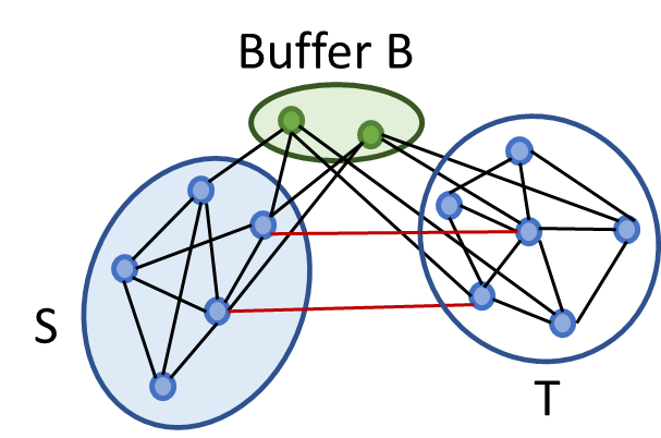
(a) Buffered partition $S,B,T=V\setminus(S\cup B)$.

(b) Buffered partitioning $(P_{1},\dots,P_{4}\|B_{1},\dots,B_{4})$

Figure 5: Left: The figure on the left shows a partition of the vertex set $V$ into three pieces $S,B$ and $T=V\setminus(S\cup B)$. Here $B$ denotes the buffer, and cost of the this cut is $\delta(S,T)$, as denoted by the edges marked in red. The edges marked in grey denote the edges between $S$ and the buffer $B$.
Right: The illustrative figure shows a $k=4$ partition $P_{1},P_{2},P_{3},P_{4}$ with buffers $B_{1},B_{2},B_{3},B_{4}$. The red edges indicate the edges $\delta(P_{1},V\setminus(P_{1}\cup B_{1}))$ that contribute to the cut corresponding to $P_{1}$. All parts $P_{1},\dots,P_{4}$ and $B_{1},\dots,B_{4}$ are disjoint.

References

- [Alo86] Noga Alon. Eigenvalues and expanders. Combinatorica, 6(2):83–96, 1986.
- [AM85] Noga Alon and Vitali D Milman. , Isoperimetric inequalities for graphs, and superconcentrators. Journal of Combinatorial Theory, Series B, 38(1):73–88, 1985.
- [AR04] Konstantin Andreev and Harald Räcke. Balanced graph partitioning. In Proceedings of the Symposium on Parallelism in Algorithms and Architectures, pages 120–124, 2004.
- [ARV09] Sanjeev Arora, Satish Rao, and Umesh Vazirani. Expander flows, geometric embeddings and graph partitioning. Journal of the ACM (JACM), 56(2):1–37, 2009.
- [BFK+14] Nikhil Bansal, Uriel Feige, Robert Krauthgamer, Konstantin Makarychev, Viswanath Nagarajan, Joseph Seffi Naor, and Roy Schwartz. Min-max graph partitioning and small set expansion. SIAM Journal on Computing, 43(2):872–904, 2014.
- [Che69] Jeff Cheeger. A lower bound for the smallest eigenvalue of the laplacian. In Proceedings of the Princeton conference in honor of Professor S. Bochner, pages 195–199, 1969.
- [CMM06] Eden Chlamtac, Konstantin Makarychev, and Yury Makarychev. How to play unique games using embeddings. In Proceedings of the Symposium on Foundations of Computer Science, pages 687–696, 2006.
- [Fil22] Arnold Filtser. Hop-constrained metric embeddings and their applications. In Proceedings of the Symposium on Foundations of Computer Science, pages 492–503, 2022.
- [FL21] Arnold Filtser and Hung Le. Clan embeddings into trees, and low treewidth graphs. In Proceedings of the Symposium on Theory of Computing, pages 342–355, 2021.
- [HHZ21] Bernhard Haeupler, D Ellis Hershkowitz, and Goran Zuzic. Tree embeddings for hop-constrained network design. In Proceedings of the Symposium on Theory of Computing, pages 356–369, 2021.
- [KBL16] Emilie Kaufmann, Thomas Bonald, and Marc Lelarge. A spectral algorithm with additive clustering for the recovery of overlapping communities in networks. In Ronald Ortner, Hans Ulrich Simon, and Sandra Zilles, editors, Algorithmic Learning Theory, pages 355–370, Cham, 2016. Springer International Publishing.
- [KLL+13] Tsz Chiu Kwok, Lap Chi Lau, Yin Tat Lee, Shayan Oveis Gharan, and Luca Trevisan. Improved cheeger’s inequality: Analysis of spectral partitioning algorithms through higher order spectral gap. In Proceedings of the Symposium on Theory of Computing, pages 11–20, 2013.
- [KLL17] Tsz Chiu Kwok, Lap Chi Lau, and Yin Tat Lee. Improved cheeger’s inequality and analysis of local graph partitioning using vertex expansion and expansion profile. SIAM Journal on Computing, 46(3):890–910, 2017.
- [KLM06] Ravi Kannan, László Lovász, and Ravi Montenegro. Blocking conductance and mixing in random walks. Combinatorics, Probability and Computing, 15(4):541–570, 2006.
- [KVV04] Ravi Kannan, Santosh Vempala, and Adrian Vetta. On clusterings: Good, bad and spectral. Journal of the ACM (JACM), 51(3):497–515, 2004.
- [LGT14] James R Lee, Shayan Oveis Gharan, and Luca Trevisan. Multiway spectral partitioning and higher-order Cheeger inequalities. Journal of the ACM (JACM), 61(6):1–30, 2014.
- [LM12] Jure Leskovec and Julian Mcauley. Learning to discover social circles in ego networks. Advances in neural information processing systems, 25, 2012.
- [LM14] Anand Louis and Konstantin Makarychev. Approximation algorithm for sparsest -partitioning. In Proceedings of the Symposium on Discrete Algorithms, pages 1244–1255, 2014.
- [LR99] Tom Leighton and Satish Rao. Multicommodity max-flow min-cut theorems and their use in designing approximation algorithms. Journal of the ACM (JACM), 46(6):787–832, 1999.
- [LRTV12] Anand Louis, Prasad Raghavendra, Prasad Tetali, and Santosh Vempala. Many sparse cuts via higher eigenvalues. In Proceedings of the Symposium on Theory of Computing, pages 1131–1140, 2012.
- [McS01] Frank McSherry. Spectral partitioning of random graphs. In Proceedings of the Symposium on Foundations of Computer Science, pages 529–537. IEEE, 2001.
- [NJW01] Andrew Y. Ng, Michael I. Jordan, and Yair Weiss. On spectral clustering: Analysis and an algorithm. In Proceedings of NeurIPS, pages 8490–856, 2001.
- [OATT22] Lorenzo Orecchia, Konstantinos Ameranis, Charalampos Tsourakakis, and Kunal Talwar. Practical almost-linear-time approximation algorithms for hybrid and overlapping graph clustering. In Kamalika Chaudhuri, Stefanie Jegelka, Le Song, Csaba Szepesvari, Gang Niu, and Sivan Sabato, editors, Proceedings of the 39th International Conference on Machine Learning, volume 162 of Proceedings of Machine Learning Research, pages 17071–17093. PMLR, 17–23 Jul 2022.
- [PSL90] Alex Pothen, Horst D. Simon, and Kang-Pu Liou. Partitioning sparse matrices with eigenvectors of graphs. SIAM Journal on Matrix Analysis and Applications, 11(3):430–452, 1990.
- [Räc08] Harald Räcke. Optimal hierarchical decompositions for congestion minimization in networks. In Proceedings of the Symposium on Theory of computing, pages 255–264, 2008.
- [RS10] Prasad Raghavendra and David Steurer. Graph expansion and the unique games conjecture. In Proceedings of the Symposium on Theory of Computing, pages 755–764, 2010.
- [RST12] Prasad Raghavendra, David Steurer, and Madhur Tulsiani. Reductions between expansion problems. In Proceedings of the Conference on Computational Complexity, pages 64–73, 2012.
- [SJ89] Alistair Sinclair and Mark Jerrum. Approximate counting, uniform generation and rapidly mixing markov chains. Information and Computation, 82(1):93–133, 1989.
- [SM00] Jianbo Shi and Jitendra Malik. Normalized cuts and image segmentation. IEEE Transactions on pattern analysis and machine intelligence, 22(8):888–905, 2000.
- [Spi07] Daniel A Spielman. Spectral graph theory and its applications. In Proceedings of the Symposium on Foundations of Computer Science, pages 29–38, 2007.
- [ST97] Horst D Simon and Shang-Hua Teng. How good is recursive bisection? SIAM Journal on Scientific Computing, 18(5):1436–1445, 1997.
- [ST07] Daniel A Spielman and Shang-Hua Teng. Spectral partitioning works: Planar graphs and finite element meshes. Linear Algebra and its Applications, 421(2-3):284–305, 2007.
- [vL07] Ulrike von Luxburg. A tutorial on spectral clustering. CoRR, abs/0711.0189, 2007.
- [YL12] Jaewon Yang and Jure Leskovec. Community-affiliation graph model for overlapping network community detection. In 2012 IEEE 12th International Conference on Data Mining, pages 1170–1175, 2012.
- [YL14] Jaewon Yang and Jure Leskovec. Structure and overlaps of ground-truth communities in networks. ACM Trans. Intell. Syst. Technol., 5(2), apr 2014.