On the Approximation of Operator-Valued Riccati Equations in Hilbert Spaces
Abstract.
In this work, we present an abstract theory for the approximation of operator-valued Riccati equations posed on Hilbert spaces. It is demonstrated here, under the assumption of compactness in the coefficient operators, that the error of the approximate solution to the operator-valued Riccati equation is bounded above by the approximation error of the governing semigroup. One significant outcome of this result is the correct prediction of optimal convergence for finite element approximations of the operator-valued Riccati equations for when the governing semigroup involves parabolic, as well as hyperbolic processes. We derive the abstract theory for the time-dependent and time-independent operator-valued Riccati equations in the first part of this work. In the second part, we prove optimal convergence rates for the finite element approximation of the functional gain associated with model one-dimensional weakly damped wave and thermal LQR control systems. These theoretical claims are then corroborated with computational evidence.
1. Introduction
In recent years, the reinforcement learning community has been rediscovering the usefulness of optimal control in the context of determining action policies. In general, reinforcement learning is involved with the direct numerical approximation of the dynamic programming principle, where the Hamilton-Jacobi-Bellman equation is solved to obtain the value of each possible state in the state space. A simplification of these equations can be made if the cost function to be minimized is quadratic and if the dynamical system governing the state is linear. This simplified problem is known in the optimal control community as the linear quadratic regulator (LQR) [39]. For these control systems, the dynamic programming principle gives an optimal feedback law which depends on the solution of Riccati equations. Aside from optimal controls, Riccati equations can be found in the Kálmán filter [31], in two-player linear quadratic games, and -control [35]. The broad implications of Riccati equations make it a very important problem to study in science, engineering, and mathematics.
Many application problems require solving the Riccati equation on infinite dimensional topologies, for example, in the control of systems whose state is governed by partial differential equations. For these systems, we call the associated Riccati equation operator-valued Riccati equations to emphasize its potentially infinite dimensional nature. It is most often the case that the state equation is approximated with a finite dimensional set of equations and that all the operators in the operator-valued Riccati equation is approximated with finite dimensional operators.
There has been a great body of literature written discussing the convergence of approximate solutions of operator-valued Riccati equations. We cite some works on this topic here [4, 34, 30, 10, 13]. While the theory presented in these works prove the pointwise convergence of approximate solutions to the exact solution, they fail to predict the rate at which approximate solutions converge. Of course, convergence rates (i.e. error estimates) are important in predicting how accurate an approximation is a priori.
Several works have provided insight on error bounds for the approximate solution of operator-valued Riccati equations for parabolic systems. In [29], it was proven that convergence is achieved for when the operators in the Riccati equation are approximated using the finite element method. Here, the differential form of the Riccati equation was used in the error analysis for deriving the error bound. The theoretical convergence rate has then been improved upon in [33], where an error bound of was proven. In this work, the mild form of the operator-valued Riccati equation was used in the analysis. Following this pattern of increasing the strength of the form of the equation analyzed, [12] used the Bochner integral form of the operator-valued Riccati equation to derive an optimal theoretical convergence rate of for -order finite element approximations. While optimal convergence rates were proven in [12], the theory was limited to steady-state operator-valued Riccati equations. It also only applies to the case for when the semigroup of the process is compact. The shortcomings of the previous approaches indicates to us that a new approach is necessary to analyze the approximation error associated with approximating the solution to the operator-valued Riccati equation.
In this work, we seek to derive a more general theory that is able to predict optimal convergence for when the process semigroup is only bounded, e.g. for both parabolic and hyperbolic partial differential equation systems. Additionally, we aim to provide results for both the time-dependent and time-independent operator-valued Riccati equations. While the focus of this work is indeed on demonstrating optimal finite element error error bounds, we emphasize that the general theory presented here can be applied to other approximation methods and also to systems that are not necessarily governed by partial differential equations. We provide some possible example applications in the beginning section of this work.
This work will first begin by defining the necessary notation and theoretical framework necessary for our discussion. Afterwards, we will then discuss the Bochner integral form of the operator-valued Riccati equations and present an abstract approximation that we study the converge of in the subsequent sections. With this, we provide some examples of potential application problems and approximation methods that can be analyzed within the framework provided in this work. After discussing these potential applications we then derive abstract error estimates that allows for the approximate solution to the operator-valued Riccati equation to be bounded by the error of the semigroup approximation for both the time-dependent and time-independent problems. Finally, we move on to present theoretical and computational results for model problems involving controlling a weakly damped wave system and a thermal control system.
2. Problem Setting
This section is concerned with establishing the theoretical framework necessary to analyze the approximation of operator-valued Riccati equations. We begin our discussion by defining the notation that we will use throughout this work. Then, we discuss the Bochner integral form of the time-dependent and time-independent operator Riccati equations and their approximations. Afterwards, we move on to state several examples to show that the operator-valued Riccati equations are pervasive in optimal control, state estimation, and game theory. And finally, we conclude this section with a brief discussion of the Brezzi-Rappaz-Raviart theorem.
2.1. Notation
In this subsection, we will define the notation that we will utilize throughout this work.
2.1.1. Bounded Linear Operators on Hilbert Spaces
In this work, we are interested in the Riccati equation posed on Hilbert spaces. To that end, let us denote as a separable Hilbert space and
as the inner product on . The norm on is then defined as
for any . Further, we will denote as the space of bounded linear operators on . The norm is then defined as
for any bounded linear operator .
The space of all compact operators on will be denoted as to be consistent with the trace-class spaces the solution to the problem of interest belong to. To be more precise,
The norm is then given by
where are the singular-values of the operator . The norm is known to coincide with the norm for the operators that we discuss in this work (i.e. for all where is a normal operator). Although the and norms are equivalent, we will denote the norm of -valued operators as to emphasize the compactness of the operator being measured. Additionally, it is known that is a two-sided *-ideal on , which can be restated as the following.
Proposition 1.
Let and , then we have that , .
Proof.
See [2, Theorem 10.69] for a proof. ∎
Symmetric operators are prevalent in our discussion on the equations studied in this work. We will denote as the space of all symmetric compact operators defined on . In mathematical notation,
It is a simple exercise to see that is a topological vector space.
The space of bounded linear operators mapping a Hilbert space to a Hilbert space will be denoted as , whose norm is defined as
for any bounded linear operator . For any bounded linear operator , we have that , where is defined as the adjoint of . Additionally, it is known that
for all and . This implies that [2, Theorem 10.11].
Let now, be a compact subset relative to a Hilbert space . Throughout this work, we will utilize the following properties regarding and .
Proposition 2.
Let be a Hilbert space and be a compact subset of . Then the following inclusions hold
Proof.
We begin by proving the first assertion presented in the above statement. From basic definitions, we have that
since . This result implies that , therefore proving our first assertion.
The second assertion is proven similarly by seeing that
again because . This result then implies that , therefore proving our second assertion. ∎
Remark 1.
Additionally, in the Lemma 7 of the technical appendix, we provide a proof that is also forms a two-sided *-ideal on . This is not a surprising result, since we already know that .
The final class of operator spaces of interest in this work are the continuous Bochner spaces , where and is an arbitrary operator space. This space is characterized by
The norm is then defined as
With the necessary functional analytic notations defined, we are now ready to discuss -semigroups and their approximations.
2.1.2. -Semigroups and Approximation on Hilbert Spaces
Let , where is the domain of , be the (infinitesimal) generator of a -semigroup . (See [27] for a discussion on -semigroups). is understood to be dense in . By definition of -semigroups, we have that there exists constants so that
| (1) |
It is known that for all and ,
Denoting be the adjoint of , then [27, Theorem 4.3] implies that is the generator of a semigroup and that is the adjoint of generated by . By extension, we have also that
for all .
Define as a subset of and as the orthogonal projection operator defined by
| (2) |
where are the basis functions of . We have assumed an infinite sum in (2) since we generally do not need any assumptions on the dimensionality of in the abstract theory that we present in this work. If is a finite dimensional space, we can simply take for all . Let now be the canonical injection operator. It is generally known that
| (3) |
The projection and injection operators will play an important role in extending operators defined on to , as we will see in the following paragraph.
Let now be the generator of a -semigroup . Again, by definition, there exists constants such that
| (4) |
We can now extend this semigroup to by defining . Since the projection and injection operators are bounded above by 1, it becomes clear that
| (5) |
where the constants are the same constants used in (4). It should be made clear that is not a -semigroup on . This is because for all . It is however a -semigroup on . The definition of becomes useful when measuring the distance between and in the metric topology. Throughout this work, we will assume that is defined in a way that it generates a parameterized sequence of -semigroup approximations so that for any
| (6) |
This then implies that
for any compact subset (as a consequence of [17, Theorem 5.3-2]). The convergence of to implies that converges to . For reference, the conditions that must be satisfied in order for (6) to be true are given in [27, Chapter 1, §7]. These semigroup approximation conditions must be verified by the reader if they wish to use the abstract results presented in this work to their application problem.
Having established the basic operator-theoretic and semigroup notations, we now move on to define the equations that we wish to approximate using the theory derived in this work.
2.2. Bochner Integral Operator-Valued Riccati Equations
The first problem that we wish to approximate the solution to is given by seeking a that satisfies
| (7) |
where for some , , are self-adjoint coefficient operators, and is again a -semigroup. This equation is shown to be equivalent to the weak differential operator Riccati equation found in, e.g. [22, Equation 6.45], as we demonstrate in Proposition 3.
From ([14, Theorem 3.6]), we have the following simplified statement of the well-posedness theorem for the Bochner integral representation of operator-valued Riccati equations.
Theorem 1 (Burns-Rautenberg).
Let be a separable complex Hilbert space, be a bounded subset with , and be a -semigroup on . In addition, assume that
-
(1)
;
-
(2)
,
where and are non-negative and self-adjoint on for all . Then the equation
where the integral is understood to be a Bochner integral, has a unique solution . Furthermore is non-negative and self-adjoint on for all .
The operator-valued Riccati equation, in most applications, is stated in its differential form. To justify the error analysis presented in this work, we must prove that the Bochner integral representation of the Riccati equation is equivalent to the differential form of the Riccati equation. We do so in the following.
Proposition 3 (Equivalence of Bochner Integral and Differential Form).
Let be a separable Hilbert space and be a -semigroup on . Then satisfies
| (8) |
if and only if satisfies
| (9) |
for all and , where is a compact time interval, , are non-negative and self-adjoint for all , and is the generator of .
Remark 2.
Equation (9) is known as the weak form of the time-dependent operator-valued Riccati equation.
Proof.
Recall that (8) is a well-posed problem by virtue of Theorem 1. We begin this analysis by testing this integral equation with test functions . This yields the following weak form of the Riccati equation
| (10) |
for almost every . It is clear that the solution of (8) satisfies (10), since strong solutions satisfy weak formulations. We then differentiate with respect to to see that
| (11) |
for almost every . This is made clear by seeing that, for any ,
| (12) | ||||
and that
| (13) | ||||
for all after applying the Leibniz integral rule and seeing that for all . Summing together (12) and (13), and then taking the inner product with the test function yields (11).
The weak form of the initial condition is then derived by evaluating (8) at and testing against , i.e.
| (14) |
for all since for all . Thus we have shown that the solution of (8) also satisfies (9). Equation (9) is then satisfied by testing (11) and (14) with a test function . Therefore, satisfying (8) also satisfies (9).
We now prove the result in the other direction. Let us now suppose that satisfies (9). Then integrating both sides of the equation gives us
for all . Theorem 1 demonstrates that the test functions are not needed in order for the integral equation (8) to be well-posed. In light of this, we see that the operator satisfying (9) also satisfies (8). This concludes the proof. ∎
The well-posedness of the Bochner integral form of the time-dependent operator-valued Riccati equation and the equivalence of the Bochner integral form to the differential form of the Riccati equation have thus been established.
2.2.1. Time-Independent Bochner Integral Riccati Equation
We have shown in the previous subsection that the Bochner integral Riccati equation is well-posed and that it is equivalent to the differential Riccati equation in the sense that the solution of both equations coincide on any time interval. We will use this equivalence to derive an integral equation that allows us to solve for the steady-state solution of the time-dependent equation. Using the commonly used notation, we define the steady-state solution of the Riccati equation as the asymptotic limit of solving as .
It is known, under the assumption of stabilizability and detectability of a system, that there exists a unique steady-state solution to the differential form of the Riccati equation [6, Part V, Theorem 3.1]. It is therefore sufficient to assume that is an exponentially stable semigroup and that are constant in time. We formalize the definition of the steady-state Bochner integral Riccati equation and show that its solution is unique in the following.
Proposition 4.
Let be a separable Hilbert space and be an exponentially stable semigroup such that there exists constants so that
Additionally, assume that are non-negative self-adjoint operators. Then, the steady-state of (8) is given by the solution of
| (15) |
Proof.
Under the assumptions given in the statement of the Lemma, we know that there exists a unique steady-state for the weak differential form of the Riccati equation given on almost all by
| (16) |
for all and any non-negative self-adjoint initial state [6, Part V, Proposition 2.2, 2.3]. From the definition of the steady-state solution [6, Part V, Proposition 2.1], we have that for all . Denoting , we observe that the system
| (17) |
is stationary (i.e. for almost all ) for all if we choose . Hence, the solution of the differential Riccati equation will remain at the steady-state if it starts at the steady state.
We then utilize Proposition 3 to see that also satisfies
for any . Taking the limit as of the above equation results in
after a change of variables since we have assumed that . ∎
It should be noted that the conditions given in Proposition 4 imply that the solution to (15) is unique. This is a direct consequence of Theorem 1. With this, we have established the well-posedness of the Bochner integral form of the time-dependent and stationary operator-valued Riccati equations. We proceed by discussing the approximation of these equations in the following subsection.
2.3. An Abstract Approximation of Operator-Valued Riccati Equations
This subsection is aimed at justifying the approach taken in the error analysis for the approximation of the Bochner integral form of the operator-valued Riccati equations. It is our goal here to demonstrate that many operator approximation methods can fit into the abstract theory that we present in this work.
2.3.1. Time-Dependent Abstract Approximation
Recall that the time-dependent problem of interest is to seek a solution that satisfies
where , , and is a -semigroup. The approximate problem we are interested in analyzing involves seeking a solution that satisfies
| (18) |
where we have approximated with . Since is, in general, not a semigroup on all of , we cannot directly apply Proposition 3 to demonstrate that (18) has a unique solution. However, we recall that , where is a semigroup on . We prove that (18) is well-posed in the following by showing that its solution is the unique extension of the solution of the approximate operator-valued Riccai equation posed on .
Proposition 5.
Proof.
We begin the analysis by taking (18) and applying the projection operator as follows
| (19) |
on . Placement of in the integral is achieved by observing that it is not a time-dependent operator. From here, we observe that
for , after seeing that the range of is , which implies that . With this, we have that
| (20) |
for on , where we have defined . Following a similar strategy, we have that
| (21) |
on with . Finally, we see that
| (22) |
where , for on after applying the above argument and seeing that the range and domain of is after inspecting (18) (The range is injected in to from and the domain is projected from onto from the definition of ). With (20), (21), and (22) we see that (18) becomes the following equation when restricting the domain and range of the equation to
| (23) |
Since , , and with denoting the space of symmetric compact operators in (compactness is preserved since is a continuous operator), Proposition 1 implies that there exists a unique that satisfies (23).
Extending the domain and range of (23) to all of then allows us to see that (23) becomes
for , where . This equation is simply (18), and hence . This establishes the existence of a solution to (18). Uniqueness then follows from the definition of and , and the uniqueness of the solution that satisfies (23). ∎
The above result then implies the solution to (18) also satisfies the following equation
| (24) |
for all and for all , where is again the generator of the approximate semigroup , with .
2.3.2. Time-Independent Abstract Approximation
Similarly, recall that the time-independent problem of interest is to seek a that satisfies
where , and is a -semigroup. The correspondent approximation is to seek a solution that satisfies
| (25) |
where again approximates . The well-posedness of (25) follows from a similar argument used in Proposition 5. Likewise, the differential form of the approximation is given by the following
| (26) |
where is again the generator to with .
2.3.3. Galerkin Approximation
The Galerkin approximation framework is likely the most utilized framework for approximating the solution to infinite dimensional equations with the solution to a finite dimensional problem. Its widespread popularity is due to its strong theoretical foundation and its flexibility in regards to choosing an approximating function space. Examples of popular Galerkin approximation methods are Finite Element methods [16, 40], Discontinuous Galerkin methods [18], Isogeometric Analysis [20], Spectral Galerkin methods [7], and Fourier Transform methods [42]. Here, we provide a brief overview of how the Galerkin approximation can be applied to the problems studied in this work.
The Galerkin approximation of a semigroup generator is given by
where is the orthogonal projection operator mapping into . The subset is chosen so that
| (27) |
where is again the canonical injection operator. The Galerkin approximation of (7) is most commonly given in the weak form by
| (28) |
for all and . It is then clear that (28) is a variant of the class of problems given by (24), where .
Since (28) is posed on a finite-dimensional topology (of dimension ), we can represent this problem by seeking a that satisfies the following equation
| (29) |
where , , and are the Galerkin approximations to and respectively. This becomes apparent after recalling (27), and seeing that the domain and range of must be in order to satisfy (28). Integrating (29) then gives us the following integral equation posed on
| (30) |
Let us now define and . It then follows from inspection, by injecting the range of (30) into , that satisfies
| (31) |
It then becomes clear that (31) satisfies the abstract form of the approximate problem given in (25). Therefore, the Galerkin approximation of the time-dependent approximation of the operator-valued Riccati equation can be analyzed within the context of the abstract theory presented in this work. A similar argument applies to the Galerkin approximation variant of the time-independent problem given in (28).
2.3.4. Asymptotic Approximation
Oftentimes, the generator is parameterized by a presumably small parameter . The operator perturbation theory [32] tells us that this operator can be represented in the following asymptotic series
where each must necessarily map into . Truncating the sum to terms gives us the asymptotic approximation
Let now and be the semigroups generated by and respectively. Then, the conditions laid out in the semigroup approximation theory presented in [27, Chapter 1, §7] must be satisfied in order for as . If convergence can be established in the limit, then as an approximation, we can simply replace with in (7) without any issue because the domain and range of and coincide. This describes the process of the asymptotic approximation of operator-valued Riccati equation. As an example, The application of asymptotic operator approximation can be found in applications involving the Born first order approximation for wave scattering in RADAR and quantum mechanical systems [15, 28].
2.4. Application Problems
This subsection will describe how the discussion presented in the preceding discussion may be applied to many important problems of practical interest. This framework may be applied to the Kálmán filter, Linear Quadratic Regulator, and Two-Player Differential Games, among other potential applications not described here (e.g. optimal control). In the following discussion we will first pose the application problem, highlight its use of a Riccati equation, and finally demonstrate how the Riccati equation fits into the abstract framework described in this section. For each of the application problems, we will present the associated time-dependent Riccati equation in the weak form and will defer the derivation of the steady-state form of these equations to the reader. The reader is reminded that the differential and Bochner integral form of the operator-valued Riccati equation are shown to be equivalent in Proposition 3.
2.4.1. Kálmán Filter
The Kálmán filter [31] has become the predominant method used in the field of state estimation. It has been so successful that state estimation practitioners have made many attempts to extend its application to estimating the state of nonlinear systems [38]. Here, we describe the Kálmán filter for linear-quadratic systems.
First, let us define and as separable Hilbert spaces associated with the state, noise, and sensor output respectively. Then the cost functional is defined as
where denotes the expectation operator with respect to the Gaussian measures associated with the random processes and representing the process and measurement noise with covariance operators and respectively, and is the solution of the following set of stochastic differential equations (stated here with an abuse of notation)
for all , where is a generator of a -semigroup, is the state noise operator, is the sensing operator. The functional gain updates the state estimate based on the difference between the sensor data and predicted sensor output for almost all . This operator is given by
where is the covariance operator given by the solution of the following operator-valued Riccati equation
for all and for all . It then becomes clear that the above equation is a variation of (9) after setting and .
2.4.2. Linear Quadratic Regulator
The linear quadratic regulator (LQR) [39] is a fundamental closed-loop control method that forces the state of a linear system to the desired terminal state. Like the Kálmán filter, the LQR has been used extensively in the control of many linear systems. It has also been applied to nonlinear systems, where the state system has been linearized about a desired set point [41, 9, 36].
Let and be separable Hilbert spaces associated with the state and control respectively. The cost function to be minimized is a quadratic functional given by
where and are weighting operators whose values can be tuned to adjust the importance of minimizing the terminal state, running cost, and the control effort respectively in the cost functional. The system to be controlled is given by
for all , where is the actuation operator. The optimal control, given as a function of , is the following
where is the functional gain given by
and is the solution of the following operator-valued Riccati equation
for all and for every . A change of variables , where transforms the terminal value problem into the initial value problem that we seek in the abstract description of the operator-valued Riccati equation. Taking , , and then allows us to see that the Riccati equation associated with LQR control can be analyzed within the framework described in this work.
2.4.3. Linear Quadratic Two-Player Differential Games
In a linear quadratic two-player differential game [8], there exists two sets of strategies and , associated with player 1 and player 2 respectively, that aims to find the saddle-point of the following cost functional
The dynamical system affected by these competing strategies is given by
The optimal strategy for each player is then given by
where is the solution of the following operator-valued Riccati equation:
for every and , where . Like in the LQR Riccati equation presented in the previous example, our desired initial-value problem is obtained through a variable transformation. Of course, setting , , and allows us to see that the Riccati equation associated with linear quadratic two-player games fits within the abstract framework of this work.
2.5. The Brezzi-Rappaz-Raviart Theorem
The Brezzi-Rappaz-Raviart (BRR) Theorem [26, Part IV, Theorem 3.3] is an important result in numerical analysis that provides a framework for deriving error bounds for the approximation of certain classes of nonlinear equations. We demonstrate in the following sections that approximations to both the time-dependent and time-independent operator-valued Riccati equation can be analyzed within this framework. A brief statement of the problem setting and the BRR theorem itself is presented in the following paragraph.
Consider the fixed point problem
| (32) |
where , belongs to a compact interval in , is a linear operator, and is a smooth mapping. Let us introduce as an operator approximation to . We then have that (32) can be approximated by the following:
| (33) |
Now suppose that there exists another space with continuous imbedding such that
| (34) |
Then, additionally under the convergence assumptions
| (35) |
and
| (36) |
the following holds.
Theorem 2 (Brezzi–Rappaz–Raviart).
Assume that conditions (34), (35), and (36) are satisfied. In addition, assume that is a operator, with bounded on all subsets of . Then, there exists a neighborhood of the origin in , and for large enough, a unique –function such that
and
Furthermore, there exists a constant independent of and with:
In the next two sections, we utilize this theorem to demonstrate that the error estimate for the approximate solution to the operator-valued Riccati equation, in principle, only depends on the the error induced by the approximate semigroup over the compact subspace characterized by the range of the coefficient operators in (7) and (15).
3. An Error Estimate for Time-Dependent Approximations
In this section, we will analyze the convergence of the approximate solutions of time-dependent operator-valued Riccati equations. Recall that on , where , we have defined the Bochner integral form of the problem as
| (37) |
where and are self-adjoint and nonnegative operators on . We wish to seek an approximation to (37) by solving the following approximating equation
| (38) |
where is approximated with .
In the following analysis, we will derive a fundamental estimate that will allow for the derivation of optimal convergence rates of in the topology. The convergence rate will depend principally on which compact subset of the coefficient operators and map to. To make this point clear in the analysis, we will take . The choice of the compact space will remain abstract and will vary depending on the application problem.
The analysis presented in the remainder of this section seeks to prove that the equations (37) and (38) have the necessary nonlinear structure necessary to utilize the Brezzi-Rappaz-Raviart theorem (Theorem 2) so that we can bound the error of the approximate solution to the exact solution by the error associated with the way the semigroup in (38) is approximated. To be more descriptive, we aim to prove that there exists a constant so that
The following analysis will begin with an inspection of the linear operator from which (37) and (38) are perturbations of. We then conclude our analysis by utilizing the derived properties of this operator to prove our desired result with the Brezzi-Rappaz-Raviart theorem (Theorem 2).
3.1. Time-Dependent Lyapunov Operator
Let us define as
| (39) |
where and .
Remark 3.
We call the Lyapunov operator, since it is the solution operator for the time-dependent variant of the Lyapunov equation shown below
This equation arises from the study of the stability of linear dynamical systems [5].
Let us now define as
| (40) |
where we again take and . It is then clear that (37) can be written succinctly as
| (41) |
We will verify the range of in the following.
Proposition 6.
Let be a separable Hilbert space, and be a compact subset of and be a compact time interval, where . Then, if , and , we have that , as defined in (40), is a mapping from into .
Proof.
We only need to show that belongs to since and , by definition. The result of this proposition follows immediately from a direct application of Corollary 1, and seeing that on for any . ∎
Similarly, we will define , as the following approximation to the Lyapunov operator
| (42) |
for all and . Likewise, (38) can be written succinctly as
| (43) |
By now, it should be clear that the convergence of will depend on the properties of the mappings , and . With this, we proceed to analyze the convergence of as .
3.2. Convergence of the Time-Dependent Lyapunov Operator Approximation
We begin this section by establishing the linearity and continuity of and in the following.
Lemma 1.
Let be a separable Hilbert space, and be -semigroups defined on a compact time interval , where and . Then for all and , we have that and are bounded linear mappings from . Furthermore, and are bounded linear mappings from .
Proof.
In this proof, we only prove the result for . It will become clear that the same sequence of steps can be repeated with instead to establish its linearity and continuity.
From the definition of (see (39)), it is easy to see that
for all , , and . Therefore, it is established that is a linear mapping, where the self-adjoint property of is established by seeing that is self-adjoint on for all .
The boundedness properties of the Lyapunov operator is then established by seeing that
after applying (1). Hence, is a bounded operator on . A continuation of the above series of inequalities yields
where we have used the fact that . With this, we have also demonstrated that is a bounded linear operator from into .
Applying the same strategy, with instead the estimate (5), establishes the linearity and boundedness of as a mapping from and into . This concludes this proof. ∎
Now that we have established that and are continuous linear operators, we can then begin to analyze the convergence of to as in the norm. The analysis is presented in the proof of the following.
Lemma 2.
Let be a separable Hilbert space and be a compact subset of . Additionally, let be a -semigroup and be an approximating sequence of -semigroups on so that
for all values in a bounded time interval , where with . Furthermore, let be defined as in (39) and (42) respectively. Then, we have that
| (44) |
for all non-negative self-adjoint operators and , and that there exists a constant such that
| (45) | ||||
for all and .
Proof.
The well-posedness and the convergence of approximate Lyapunov operators, in pointwise and uniform sense, to the exact Lyapunov operator was established in the results presented in this subsection. In the final part of this section, we will apply Theorem 2 to determine that the error of the approximate solution of the operator-valued Riccati equation is bounded by the semigroup approximation error.
3.3. Approximation Error
Throughout this subsection, we will denote our function spaces of interest in the following manner
to make the application of Theorem 2 easier to visualize. We note that is a continuous embedding by recalling the definition of these spaces.
We begin by seeing again that (37) and (38) can be written in a fixed-point form as
respectively. The linearity and boundedness of was established in Lemma 1. It is then easy to see from the definition of that it is infinitely Fréchet with respect to . The first Gatéux derivative of with respect to is given explicitly as
| (46) |
for any test operator . Since and that is an element in every space, we can see that as a result of Lemma 7. Finally, we restate the pointwise and uniform convergence result that we have derived in Lemma 2 in our new notation below, i.e.
A direct comparison of the above observations against the conditions stated in §2.5 allow us to apply the Brezzi-Rappaz-Raviart theorem (Theorem 2) to see that there exists a constant such that
after recalling that . Bounding this inequality with (45) yields the first main result of this work.
Theorem 3.
Let be a separable Hilbert space and be a compact subset of . Additionally, let be a -semigroup and be an approximating sequence of -semigroups on so that
for all values in a bounded time interval , where with . Furthermore, let be defined as in (39) and (42) respectively. And finally, let be defined as in (40). Then, we have that there exists a constant so that
where are the solutions of the operator-valued Riccati equation (37) and its approximation (38) respectively.
Remark 4.
In practice, the above result needs to be supplemented with additional analysis to resolve the time approximation error associated with time-stepping techniques. This error can be accounted for by simply utilizing the Minkowski inequality and applying known approximation results for time-stepping, i.e.,
| (47) |
where we have introduced as the solution approximation where both space and time-approximation has been applied. The error between and can then be bounded with existing results, under sufficient smoothness of with respect to (see [37, Chapter 11]).
With this, we have established an abstract error estimate for the solution of an approximation to time-dependent operator-valued Riccati equations. This estimate shows that the error bound on the approximate solution to time-independent operator Riccati equations is a function of the error of the semigroup approximation used in the approximate equation. The implication of this result is that many previous results in the approximation of time-dependent processes can be applied in deriving the error bound of the approximate solution of the Riccati equation in a control and/or estimation system in question. We will qualify this claim in §5. In the next section, we demonstrate in Theorem 4 that this observation can be applied to the time-independent variant of operator-valued Riccati equations.
4. An Error Estimate for Time-Independent Approximations
In this section, we will continue our analysis by deriving an abstract error estimate for approximate solutions to the time-dependent operator Riccati equation. Most of the analysis presented in this section is analogous to what we have already presented in the previous section. We begin by recalling again that the steady-state form of the operator Riccati equation is given as
| (48) |
where is an exponentially stable semigroup satisfying , are compact, non-negative, and self-adjoint operators on . We will again make the range of and explicit in this analysis by indicating that , where is a compact subset. For reference, it was demonstrated in Lemma 4 that (48) is a well-posed problem.
The corresponding approximation to (48) is given by
| (49) |
where is an approximation to satisfying . The analysis presented below implies that the semigroup approximation must satisfy the known preservation of exponential stability (POES) property in order for there to exist a bounded approximate solution to (49) [4].
The analysis presented in this section will follow the same structure as the analysis presented in Section 3. It is our goal to attempt to present our analysis in this section succinctly since its underlying logic is similar to (and simpler than) what we have presented in the previous section. To that end, we will first define the steady-state Lyapunov operator and its approximation and show that they are linear and bounded operators on . Then, we move to demonstrate that the approximate Lyapunov operator converges to the exact Lyapunov operator in the pointwise and uniform sense on compact subsets. And finally, we apply the Brezzi-Rappaz-Raviart theorem (Theorem 2) to derive the main result of this section.
4.1. Time-Independent Lyapunov Operator
Let us define as
| (50) |
for all . We call this operator the steady-state Lyapunov operator. Additionally, let us define as
| (51) |
where . It is then clear that we can represent (48) by
| (52) |
This representation indicates that Theorem 2 is applicable to (48). We verify the range of in the following.
Proposition 7.
Let be a separable Hilbert space and be a compact subset of . If , then is a mapping from to .
Proof.
We need to only show that for any . This is easily seen by applying Lemma 7 and seeing that by definition. ∎
The approximation of interest to the steady-state Lyapunov operator given in (50) is defined as
| (53) |
Similarly, the approximate steady-state operator Riccati equation (49) can be written as
| (54) |
We now verify the linearity and boundedness of and in the following.
Lemma 3.
Proof.
We begin this proof by observing that on for any . It is then clear from the definition of that
for all and . Hence, is a linear operator.
The boundedness of on , is established by seeing that
for all .
The above analysis applies to as well, since is a -semigroup assumed to preserve exponential stability. This concludes the proof. ∎
4.2. Convergence of Time-Independent Lyapunov Operator Approximations
We now move forward to analyze the convergence of in the following.
Lemma 4.
Let be a separable Hilbert space and be a compact subset of . Additionally, let be an exponentially stable -semigroup and be an approximating sequence of -semigroups so that
for any . Under these assumptions, we observe that
| (55) |
and
| (56) |
where , and the operators are defined as in (50) and (53) respectively.
Proof.
We begin the proof by seeing that is a bounded sequence as a consequence of Lemma 3 since is assumed to be exponentially stable for any . This observation validates the notion of convergence of .
From the definition of and , we see that
Taking the norm on both sides of the above equation then gives us the following inequality.
We establish (55) by seeing that and are bounded and that is pointwise convergent by Lemma 8.
We continue bounding the inequality above by seeing that
by observing that
for any , and that and . Thus (56) is verified. This concludes the proof. ∎
4.3. Approximation Error
In this section, we will utilize the Brezzi-Rappaz-Raviart Theorem (Theorem 2) to derive an error estimate for the approximation of the operator-valued steady state Riccati equation on Hilbert spaces. To that end, we begin by defining
From the definition of , we see that is infinitely Fréchet differentiable. Further, we see that
therefore for any . In Lemma 4, we have shown that
and
With these observations, we see that there exists a constant that satisfies
after applying Theorem 2 and recalling that . Applying (56) then allows us to establish the main result of this section.
Theorem 4.
With this result, we conclude the analysis for the approximation of the time-dependent operator Riccati equation. Like in the approximation theorem presented in the previous section (Theorem 3), we observe that the error bound of the approximate solution to the Riccati equation is a function of the error of the semigroup approximation. Similarly, we can utilize the many existing results on the approximation of time-dependent processes to derive error estimates for time-independent operator Riccati equations. We will apply this knowledge in the following section.
5. One Dimensional Model LQR Control Problems
In this section, we demonstrate the applicability of the theory derived in the earlier sections of this work to the finite element approximation of LQR control systems approximated with the finite element method. Here, the finite element method is applied a thermal control system and a weakly damped wave control system, where the time-dependent operator-valued Riccati equation is approximated in the first model problem and the time-independent operator-valued Riccati equation is approximated in the second model problem. Because the operator norm is difficult to compute, we instead choose to compute the error of the functional gain associated with the optimal feedback law associated with the approximate control system. We demonstrate in both model problems that the error of the approximate functional gain is dependent on the error of the approximate solution to the relevant Riccati equation. We conclude each subsection by presenting convergence rates computed from the computational implementation of the model problems.
5.1. Notation
In the model problems considered in the following, the problem domain will be defined as the one-dimensional interval , and the boundary as the endpoints . We then define
as the duality pairing between and , where is a topological vector space of vectors defined on , and denotes the dual space associated with . The norm on is then denoted .
Let now be a second topological vector space. The tensor product space can then be defined as
where and are topological vector spaces. The norm on can then defined by
for all .
The topological vector spaces of interest for the discussion presented here are the Sobolev spaces and . These spaces are defined as follows:
where denotes the -th partial derivative with respect to . The Sobolev norms are then defined as
Additionally, we are interested in the space , which is defined as
This space is the solution space of the Poisson equation with homogeneous Dirichlet boundary conditions.
We use the Finite Element Method (see, e.g., [40]) in the numerical approximations presented in the subsections below. One dimensional piecewise Lagrange polynomials [11, Chapter 3, Section 1] of arbitrary order are chosen as the approximation space. The domain is segmented into disjoint line segments of equal length . On , the piecewise Lagrange polynomial approximation space is then defined as
| (57) |
where denotes the space of continuous functions defined on and denotes the space of polynomials of order defined over . The dimension of is then denoted as . We will then denote as an admissible basis of . Furthermore, we define the space
| (58) |
which consists of all functions belonging to that are zero on . The dimensionality of this space is then since we do not require any approximating polynomials centered at the endpoints of the domain.
5.2. Finite-Horizon LQR Control of a 1D Thermal Process
5.2.1. Problem Definition
In this example problem, we consider an one dimensional thermal control system whose state is controlled by adjusting the heat flux into and out of the interior domain. Additionally, we will let be the finite time domain on which we want to exercise the control law. The mathematical model for this system is then given by
| (59) |
where is the control input and is the actuator function. The coefficients determines the rate of thermal dissipation within the domain and out of the domain respectively. Here, we apply the LQR methodology and choose an optimal control that minimizes the following cost functional
| (60) |
where .
For this problem, we will define and as the following
We will now map the model equations into the infinite-dimensional state space setting. To that end, let us now define as the state space for the thermal control problem and as the generator , where . The theory behind the generation of the dissipative semigroup from can be found in [25, Chapter 7.4]. The compact space of interest for this problem is then , where we have assumed that . The compactness of relative to is verified by the Rellich-Kondrachov theorem [1, Chapter 6]. We now write the state space representation of the model problem as
which is well-defined for all and since we have shown that the range of and are in . The correspondent optimal feedback law can be given by
where and satisfies the following weak time-dependent algebraic Riccati equation
for all . The theory discussed in §3 applies to this example problem, since , by definition.
5.2.2. Finite Element Approximation with Piecewise Lagrange Elements
The finite element approximation of (59) is given by seeking a that satisfies
| (61) |
for all and , where
is the bilinear form associated with the diffusion operator . Here, the homogeneous Neumann boundary condition is enforced naturally through integration-by-parts and setting the boundary terms to zero. The solution can then be represented as
where is a set of functions representing the basis of the approximation space . The coefficients is then the solution of the following matrix system
where
with
The resultant cost functional to be minimized is then given in matrix form as
| (62) |
where
This cost functional is derived by substituting with and with in (60) and recalling that .
The optimal feedback law for the finite element matrix control system is then given by
where is the vector representation of the functional gain given by
and is the solution of the following matrix Ricccati equation
for all . The functional gain of the matrix system can then be defined as a function in by setting and then defining , where are the elements of the vector . In functional form, we may write the functional gain as
With this, we move on to present the main result of this section.
Lemma 5.
Let and , then there exists a constant such that
where and are the functional gains associated with the optimal feedback laws for the infinite dimensional control system and its finite element approximation respectively.
Proof.
For the purpose of analysis only, we may equivalently represent the finite element weak problem (61) as
for all , where the operator is defined by
for all . Here, since homogeneous Neumann boundary condition is enforced implicitly as a natural condition. The actuator operator can be simply taken as the simple projection of , i.e.
where is the orthogonal projection operator associated with the approximation space . Then, the optimal feedback law for the state space representation of the finite element approximation can then be given as
where is the solution of the following operator-valued Riccati equation
for all and .
From Theorem 3, we have that there exists a constant so that
where is the -semigroup generated by , and is the -semigroup approximation generated by . Applying Lemma 10 allows us to see that there exists a constant so that
where is verified by inspecting the definition of and the smoothness assumption made on . Following this, we have that there exists a constant
after seeing that for all as a consequence of the one dimensional Lagrange interpolation error estimate given in [24, Proposition 1.12]. Putting these error bounds together allows us to see that
Thus proving the error bound presented in this Lemma. ∎
This concludes the analytical discussion regarding the theoretical error estimate for the finite element approximation of the model thermal control system. We corroborate the error estimate for the functional gain in the computational results presented in below.
5.2.3. Computational Results
In this computational illustration, we set , , , and . With these parameters, the time-dependent matrix Riccati equation was solved using the trapezoidal time-stepping method [11, §5.4] with a time-step of . The linalg.solve_continuous_are() function in the SciPy numerical library was used to solve the matrix Riccati equation at every implicit time step. The terminal condition was taken to be .
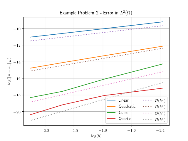
The functional gain error is plotted in Figure 1 with respect to the norm, where we have compared the finite element solution to a spectral element solution on a single element with a 128-th order Lagrange polynomial basis defined on the Lobatto quadrature points. We observe good agreement between the numerically computed errors and our theoretical results, albeit with numerical precision error on the convergence of the quartic finite element approximation.
We now move forward to discuss the error estimate for the finite element approximation of our model damped wave control system.
5.3. Infinite-Horizon LQR Control of a 1D Weakly Damped Wave System
5.3.1. Problem Definition
The model problem we approximate in this section is given by
| (63) |
subject to the 1D weakly damped wave system
for some arbitrary initial conditions , and . The functions and are chosen to be smooth for this example and we require that they are zero on , i.e. . The homogeneous boundary condition here is required in order to derive an optimal error estimate because of the way the Galerkin projection is utilized in the error analysis for the finite element approximation for the wave equation (see [3] for a complete discussion). Here will denote the polynomial order of the approximation space used in the finite element approximation.
We can map this control problem into the state space form required by our theory by setting
where we have denoted as the identity operator in . We can write the above control system in the following form
subject to
for all , where we have chosen , , and . This choice of and is required in order for to generate an exponentially stable -semigroup (e.g., see [21]). With this, it is clear that this example problem falls into the set of problems presented in §2.4.2. The associated Riccati equation for this model problem is then given in the weak form by
for all . It is then clear that and are operators belonging to , where . The choice of is derived from our earlier definition of the functions and as well as the analysis given in §B.2. The optimal feedback law for this model control system is then given by
| (64) |
for all , where is the functional gain defined as .
5.3.2. Finite Element Approximation with Piecewise Lagrange Elements
The approximation space associated with this model problem is given by
This approximation space is chosen since must be zero on because and is zero on for all . An inspection indicates that and hence the orthogonal projection operator is well defined.
In the finite element approximation of the weakly damped wave system, the approximate system is defined in the weak form by
where
are the finite element approximation of and respectively, given time-dependent coefficients , and
is a bilinear form mapping any to . It then follows, by the finite dimensional nature of the space , that the finite element description of the approximate problem can be written in an equivalent matrix form given by
where for ,
with being a column vector. Denoting
we may write the finite dimensional problem in the following block form
| (65) |
where , , and .
With this, we wish to choose that minimizes following cost functional
| (66) |
where is a row vector with for . The matrix form of the cost functional given in (66) arises by replacing with and with in (63). The optimal feedback law for the finite element approximation of the control system is then given in matrix form by
where and is the solution of the following matrix Riccati equation
| (67) |
We now wish to represent the optimal feedback law in the functional sense, where
The approximate functional gain as an element of by first defining , where the coefficients are computed using
where we have denoted . The functional form is then given by setting
With this, we can now prove that converges to with an optimal order of convergence.
Lemma 6.
Let and for all . If , then there exists a constant so that
where are the functional gains associated with the optimal feedback control law for the infinite dimensional control system (64) and its finite element approximation respectively.
Proof.
From the definition of , we see that
where . From Theorem 4, we observe that
as a consequence of Lemma 12. We observe that is bounded in from the smoothness assumptions made on and .
We continue by seeing that
after bounding the error associated with the projection onto by the error associated with one-dimensional Lagrange interpolation. ([24, Proposition 1.12]). With this, it becomes clear that there exists a constant so that
This concludes the proof. ∎
5.3.3. Computational Results
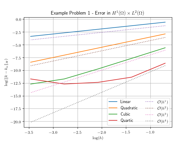
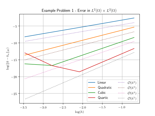
In the computational illustration, the author’s personal code was utilized to generate the operator matrices defined above. The linalg.solve_continuous_are() function in SciPy was utilized to solve (67). We set , , and . With these parameters, the matrix Riccati equation was solved and the functional gain was computed. The functional gain error is plotted in Figure 2 with respect to the norm and norm, where we have compared the finite element solution to a spectral element solution on a single element with a 128th order Lagrange polynomial basis defined on the Lobatto quadrature points. We observe good agreement between the numerically computed errors and our theoretical results, albeit with numerical precision error past .
6. Conclusion
In this work, we have presented an abstract theory for the approximation of operator-valued Riccati equations. This theory indicates that the error of the solution of these equations, in the time-dependent and time-independent forms, is bounded by error associated with the governing semigroup approximation. This result was derived through the use of the Brezzi-Rappaz-Raviart theorem on the equivalent Bochner integral form of the operator-valued Riccati equations. This form is particularly useful because it possesses the necessary fixed-point structure for applying the Brezzi-Rappaz-Raviart theorem. It was shown at the beginning of this work that the abstract theory presented can be used on many different problems and also on many different approximation methods.
In the model problems presented, we have shown that the finite element approximation of the functional gains, under certain smoothness conditions, are expected to converge to the exact functional gain with optimal order. Correspondingly, our computational result corroborates these theoretical findings.
7. Future Work
While we believe that the theory presented in this work has wide-reaching implications, we are also aware of several theoretical shortcomings. The most notable shortcoming is the treatment of unbounded operators. These operators typically occur in e.g. boundary and point control and observation systems. Our work cannot be applied to these problems since the unbounded operators violate the compactness assumptions required by our theory. A possible path forward is to demonstrate that the Bochner integral form of the operator-valued Riccati equation is well-posed for when the coefficient operators are unbounded, and then adapting the analysis presented in this work to that general case. We plan on exploring in this direction in future works.
References
- [1] Robert A Adams and John JF Fournier. Sobolev spaces. Elsevier, 2003.
- [2] Sheldon Axler. Measure, integration & real analysis. Springer Nature, 2020.
- [3] Garth A. Baker. Error estimates for finite element methods for second order hyperbolic equations. SIAM Journal on Numerical Analysis, 13(4):564–576, 1976.
- [4] H. T. Banks and K. Kunisch. The linear regulator problem for parabolic systems. SIAM Journal on Control and Optimization, 22(5):684–698, 1984.
- [5] Maximilian Behr, Peter Benner, and Jan Heiland. Solution formulas for differential sylvester and lyapunov equations. Calcolo, 56(4):51, 2019.
- [6] Alain Bensoussan, Giuseppe Da Prato, Michel C Delfour, and Sanjoy K Mitter. Representation and control of infinite dimensional systems, volume 1. Springer, 2007.
- [7] Christine Bernardi and Yvon Maday. Spectral methods. Handbook of numerical analysis, 5:209–485, 1997.
- [8] Pierre Bernhard. Linear-quadratic, two-person, zero-sum differential games: necessary and sufficient conditions. Journal of Optimization Theory and Applications, 27(1):51–69, 1979.
- [9] RI Boby, H Mansor, TS Gunawan, and S Khan. Robust adaptive lqr control of nonlinear system application to 3-dof flight control system. In 2014 IEEE International Conference on Smart Instrumentation, Measurement and Applications (ICSIMA), pages 1–4. IEEE, 2014.
- [10] Jeff Borggaard, John A Burns, Eric Vugrin, and Lizette Zietsman. On strong convergence of feedback operators for non-normal distributed parameter systems. In 2004 43rd IEEE Conference on Decision and Control (CDC)(IEEE Cat. No. 04CH37601), volume 2, pages 1526–1531. IEEE, 2004.
- [11] Richard L Burden, J Douglas Faires, and Annette M Burden. Numerical analysis. Cengage learning, 2015.
- [12] John A Burns and James Cheung. Optimal convergence rates for galerkin approximation of operator riccati equations. Numerical Methods for Partial Differential Equations, 2022.
- [13] John A Burns and Kevin P Hulsing. Numerical methods for approximating functional gains in lqr boundary control problems. Mathematical and Computer Modelling, 33(1-3):89–100, 2001.
- [14] John A Burns and Carlos N Rautenberg. Solutions and approximations to the riccati integral equation with values in a space of compact operators. SIAM Journal on Control and Optimization, 53(5):2846–2877, 2015.
- [15] Margaret Cheney and Brett Borden. Fundamentals of radar imaging. SIAM, 2009.
- [16] Philippe G Ciarlet. The finite element method for elliptic problems. SIAM, 2002.
- [17] Philippe G Ciarlet. Linear and nonlinear functional analysis with applications, volume 130. Siam, 2013.
- [18] Bernardo Cockburn, George E Karniadakis, and Chi-Wang Shu. Discontinuous Galerkin methods: theory, computation and applications, volume 11. Springer Science & Business Media, 2012.
- [19] Monica Conti, Lorenzo Liverani, and Vittorino Pata. On the optimal decay rate of the weakly damped wave equation. Communications on Pure and Applied Analysis, 21(10):3421–3424, 2022.
- [20] J Austin Cottrell, Thomas JR Hughes, and Yuri Bazilevs. Isogeometric analysis: toward integration of CAD and FEA. John Wiley & Sons, 2009.
- [21] Steven Cox and Enrique Zuazua. The rate at which energy decays in a damped string. Communications in partial differential equations, 19(1-2):213–243, 1994.
- [22] Ruth F Curtain and Hans Zwart. An introduction to infinite-dimensional linear systems theory, volume 21. Springer Science & Business Media, 2012.
- [23] Todd Dupont. -estimates for galerkin methods for second order hyperbolic equations. SIAM Journal on Numerical Analysis, 10(5):880–889, 1973.
- [24] Alexandre Ern and Jean-Luc Guermond. Theory and practice of finite elements, volume 159. Springer, 2004.
- [25] Lawrence C Evans. Partial differential equations, volume 19. American Mathematical Society, 2022.
- [26] Vivette Girault and Pierre-Arnaud Raviart. Finite element methods for Navier-Stokes equations: theory and algorithms, volume 5. Springer Science & Business Media, 2012.
- [27] Jerome A Goldstein. Semigroups of linear operators and applications. Courier Dover Publications, 2017.
- [28] JE Gubernatis, E Domany, JA Krumhansl, and M Huberman. The born approximation in the theory of the scattering of elastic waves by flaws. Journal of Applied Physics, 48(7):2812–2819, 1977.
- [29] Kazufumi Ito. Strong convergence and convergence rates of approximating solutions for algebraic riccati equations in hilbert spaces. In Distributed Parameter Systems, pages 153–166. Springer, 1987.
- [30] Kazufumi Ito and Kirsten A Morris. An approximation theory of solutions to operator riccati equations for control. SIAM journal on control and optimization, 36(1):82–99, 1998.
- [31] Rudolph Emil Kalman. A new approach to linear filtering and prediction problems. 1960.
- [32] Tosio Kato. Perturbation theory for linear operators, volume 132. Springer Science & Business Media, 2013.
- [33] Michael Kroller and Karl Kunisch. Convergence rates for the feedback operators arising in the linear quadratic regulator problem governed by parabolic equations. SIAM journal on numerical analysis, 28(5):1350–1385, 1991.
- [34] Irena Lasiecka and Roberto Triggiani. Differential and algebraic Riccati equations with application to boundary/point control problems: continuous theory and approximation theory. Springer, 1991.
- [35] C. McMillan and R. Triggiani. Algebraic riccati equations arising in game theory and in -control problems for a class of abstract systems. In W.F. Ames, E.M. Harrell, and J.V. Herod, editors, Differential Equations with Applications to Mathematical Physics, volume 192 of Mathematics in Science and Engineering, pages 239–247. Elsevier, 1993.
- [36] Lal Bahadur Prasad, Barjeev Tyagi, and Hari Om Gupta. Optimal control of nonlinear inverted pendulum system using pid controller and lqr: performance analysis without and with disturbance input. International Journal of Automation and Computing, 11:661–670, 2014.
- [37] Alfio Quarteroni, Riccardo Sacco, and Fausto Saleri. Numerical mathematics, volume 37. Springer Science & Business Media, 2010.
- [38] Maria Isabel Ribeiro. Kalman and extended kalman filters: Concept, derivation and properties. Institute for Systems and Robotics, 43(46):3736–3741, 2004.
- [39] Robert F Stengel. Optimal control and estimation. Courier Corporation, 1994.
- [40] Gilbert Strang, George J Fix, and DS Griffin. An analysis of the finite-element method. 1974.
- [41] Russ Tedrake. Lqr-trees: Feedback motion planning on sparse randomized trees. 2009.
- [42] Jaroslav Vondřejc, Jan Zeman, and Ivo Marek. An fft-based galerkin method for homogenization of periodic media. Computers & Mathematics with Applications, 68(3):156–173, 2014.
Appendix A Technical Lemmas
In this section, we present the technical lemmas that we will use throughout the analysis presented in this work. We begin by demonstrating that forms a two-sided *-ideal (stated in a different manner).
Lemma 7.
Let be a separable Hilbert space and be a compact subset of . In addition, let and , Then .
Proof.
The following result is then easily proven.
Corollary 1.
Let be a separable Hilbert space and be a compact subset of , and be a compact subset of . Additionally, let and . Then .
Proof.
We conclude this section by seeing that the pointwise convergence of approximate semigroups also applies to when the semigroup acts on an operator belonging to .
Lemma 8.
Let be a separable Hilbert space and be a -semigroup. In addition let be an approximating sequence of -semigroups such that
Then we have that
| (68) |
and
| (69) |
for all and .
Appendix B Error Estimates for Finite Element Approximation of Semigroups
In this section, we will present results on the error estimates for finite element methods for the heat and the weakly damped wave equation for when the solution operator of these equations are represented as a semigroup. We will begin by analyzing the heat semigroup approximation error and then move on to analyze the weakly damped wave semigroup approximation error. For simplicity, we will consider only the one-dimensional case to avoid the theoretical technicalities regarding geometric approximation. See [40] for a discussion on how curved domains can be theoretically addressed. We remark that the majority of the analysis presented here can likely be extended to the case where the domain of the partial differential equation is curved without serious issues. The notation used in §5.3 and §5.2 will be used in the following discussion.
B.1. Finite Element Approximation of the Thermal Semigroup
In this analysis, we will carry over the notation used in §5.2. Recall that we have defined for this test problem, where . It is known that generates an exponentially stable semigroup [25, §7.4]. Letting , for any , we have that is the solution of the following equation
| (70) |
Additionally, it is known that also generates an exponentially stable semigroup . We extend the domain and range of through an injection and projection process, i.e., . Letting , for any , we have that is the solution of the following weak equation
for all and .
With these notions defined, we are now ready to begin deriving an error bound on . We start with the following necessary result.
Lemma 9.
Let be the parabolic semigroup generated by , then we have that
for all .
Proof.
Taking the -th order partial derivative with respect to on both sides of (71) results in
Switching the order of differentiation then allows us to see that
| (71) |
where we have denoted . It then follows that
which proves the result of this Lemma. ∎
We now move on to derive the main result of this analysis in the following.
Lemma 10.
Let be the parabolic semigroup generated by , and be its finite element approximation, then we have that there exists a constant so that
where is the fundamental rate of dissipation of the parabolic semigroup and is the polynomial order of the finite element approximation space.
Proof.
Following the analysis presented in [40, Theorem 7.1], we have that
We begin by seeing that
as a consequence of applying Lemma 9 to the definition of the norm. We then see that
which follows again from applying Lemma 9, and equation (71). It then follows that
We then arrive at the result of this Lemma by recalling that and that , and then finally applying the definition of the operator norm. ∎
We have shown above that the classical finite element error estimate for parabolic equations can be used to derive uniform error estimates for the approximate semigroup in the operator norm. We will derive a similar estimate for the approximation of hyperbolic semigroups in the following subsection.
B.2. Finite Element Approximation of the Weakly Damped Wave Semigroup
Here, we present results pertaining to the finite element approximation error estimates for the weakly damped wave semigroup. The notation used here will be carried over from §5.3. Recall that we have set with . It is known that generates an exponentially stable semigroup [19] which we denote . Letting for any , we have that is the solution of the following weakly damped wave equation
| (72) |
where we have denoted . Additionally, it is known that also generates an exponentially stable semigroup . The domain and range of can then be extended through an injection and projection process, i.e., . Setting , for any , we have that satisfies the following set of weak equations
for all . We now define the following differential operator for notational convenience
for any with and possessing at least and weak derivatives respectively. We now move forward to derive the first result of this section.
Lemma 11.
Let be the weakly damped wave semigroup, then we have that
| (73) |
for all .
Proof.
First, we see that is well defined since for any from the definition of Sobolev spaces. This is necessary since . The remainder of the proof follows using the same argument as in the proof of Lemma 9.
Next, taking the -th order partial derivative with respect to on both sides of (72) results in
after interchanging the order of partial differentiation. This then allows to see that
for any . This concludes the proof. ∎
We now move on to derive an error estimate on the finite element approximation of the weakly damped wave semigroup in the following.
Lemma 12.
Let be the weakly damped wave semigroup generated by , and be its finite element approximation, then we have that there exists a constant so that
where is the fundamental rate of dissipation of the parabolic semigroup and .
Proof.
In this analysis, we take as any arbitrary vector and with . Lemma 11 then implies that .
From the analysis presented in [23], we have that
Seeing that , we observe that
after applying the embedding inequality . Applying Lemma 11 and the exponential stability of allows us to see that
Putting this all together, we observe that
We conclude the proof by seeing that
and applying the definition of the operator norm. ∎