Dynamic Bilevel Learning with Inexact Line Search

Abstract

In various domains within imaging and data science, particularly when addressing tasks modeled utilizing the variational regularization approach, manually configuring regularization parameters presents a formidable challenge. The difficulty intensifies when employing regularizers involving a large number of hyperparameters. To overcome this challenge, bilevel learning is employed to learn suitable hyperparameters. However, due to the use of numerical solvers, the exact gradient with respect to the hyperparameters is unattainable, necessitating the use of methods relying on approximate gradients. State-of-the-art inexact methods a priori select a decreasing summable sequence of the required accuracy and only assure convergence given a sufficiently small fixed step size. Despite this, challenges persist in determining the Lipschitz constant of the hypergradient and identifying an appropriate fixed step size. Conversely, computing exact function values is not feasible, impeding the use of line search. In this work, we introduce a provably convergent inexact backtracking line search involving inexact function evaluations and hypergradients. We show convergence to a stationary point of the loss with respect to hyperparameters. Additionally, we propose an algorithm to determine the required accuracy dynamically. Our numerical experiments demonstrate the efficiency and feasibility of our approach for hyperparameter estimation in variational regularization problems, alongside its robustness in terms of the initial accuracy and step size choices.

65K10, 90C25, 90C26, 90C06, 90C31, 94A08

1 Introduction

In this work, we consider supervised hyperparameter learning formulated as a bilevel learning problem [16, 37] where our goal is to solve

(1a) $$\min_{\theta\in\mathbb{R}^{d}}\{f(\theta) \coloneqq\frac{1}{M}\sum_{i=1}^{M}g_{i}(\hat{x}_{i}(\theta))+r(\theta)\}$$

(1b) $$s.t.\quad{\hat{x}_{i}(\theta)} \coloneqq\arg\min_{x\in\mathbb{R}^{N}}\Phi_{i}(x,\theta),\quad i=1,\dots,M,$$

where each $\Phi_{i}$ is smooth in $x$ and $\theta$, and strongly convex in $x$. The upper level functions $g_{i}$s and $r$ in (1a) are also smooth and convex. The upper level functions $g_{i}$s are a measure of goodness of the solution of the lower level problem (1b). For example, they may take the form $g_{i}(x)=\|x-\bar{x}_{i}\|^{2}$ where $\bar{x}_{i}$ is the ground truth and the desired solution of the lower-level problem for a suitable set of training data $\{(\bar{x}_{i},y_{i})\}_{i=1}^{M}$.

Problems of the form (1) arise in many areas of science when the task at hand is modeled using variational regularization approaches, which are standard in the fields of image reconstruction, image processing, machine vision, and data science. For instance, one can learn the weights of the regularizer in regression [35], or the regularizer [25, 15, 34] for image denoising, deblurring, inpainting, segmentation, and single-image super-resolution by formulating them as the problem (1). Moreover, the parameters of more sophisticated data-adaptive regularizers which can have up to millions of parameters like input-convex neural networks (ICNN) [31, 1] and convex-ridge regularizer neural networks (CRR-NN) [21] can be learned in the same way. The relevance of bilevel learning problems in variational regularization methods is not restricted to regularizers. It can also be employed to learn the parameters in analytical deep priors [17, 2], and the sampling operator in MRI [39].

In order to solve the problem (1), model-free approaches such as grid search and random search [7] can be used when there are a small number of hyperparameters, and the space of hyperparameters is bounded and small. Model-based approaches like Bayesian methods [20] and derivative-free optimization [13, 12, 18] are efficient in solving the bilevel problem (1) when a small number of hyperparameters are involved. However, we are interested in scalable methods that can solve bilevel problems potentially with up to millions of parameters. Hence, in this work, we consider gradient-based methods as a scalable approach.

In the gradient-based approach, a first-order [3, 14] or quasi-Newton [33] algorithm is employed to solve the lower-level problem (1b). Then, gradient descent is applied to the upper-level problem (1a) after computing the gradient $\nabla f(\theta)$ (also referred to as the hypergradient) with respect to parameter $\theta$. Under certain regularity assumptions, when the problem is sufficiently smooth [18, 35], the hypergradient can be calculated by utilizing the implicit function theorem [18] or by using automatic differentiation [30]. However, due to the usage of numerical solvers and the large-scale nature of the problems of interest, computing the exact hypergradient is not realistic [19]; hence, it should be approximated with an accuracy that leads to optimization with inexact hypergradients in the upper-level problem (1a).

Although much work has been done on different methods of finding the hypergradient and its error bound, the convergence theorems for hyperparameter optimization with an inexact hypergradient have only been studied assuming that we have a small enough fixed step size [35]. However, since the closed-form solution of the lower-level problem (1b) is not available, estimating the Lipschitz constant of the hypergradient, and consequently, employing a method with the largest possible fixed step size is not realistic. Moreover, convergence theory requires a summable sequence of accuracies, which is overly restrictive and can limit the practical performance of the method.

At first glance, the backtracking line search seems reasonable to address this issue, but it requires evaluating the exact upper-level objective value, which is not possible since we only have access to an approximate lower-level solution. Besides, line search requires the approximated hypergradient to be a descent direction, which is not obvious. Moreover, it has been shown empirically (e.g., [19]) that inexact gradient descent on the parameters can make progress even if the accuracy does not increase under a priori assumptions like summability.

In this work, we introduce a scheme to ensure that an inexact hypergradient is a descent direction. We then propose a modified inexact backtracking line search that employs the inexact hypergradient alongside only inexact function evaluations that guarantee a sufficient decrease in the exact upper-level function. Subsequently, we propose an algorithm that dynamically chooses the required accuracy for having a hypergradient as a descent direction and the sufficient decrease condition to hold as well as performing the backtracking line search. Our numerical results compare the performance of our algorithm with state-of-the-art algorithms in solving problems of the form (1) for a wide range of problems. Importantly, our numerical experiments indicate a significant improvement in terms of finding an optimal loss value with the same computational cost compared to Hyperparameter optimization Approximate Gradient (HOAG) [35] with adaptive step size and dynamic derivative-free optimization algorithm (DFO-LS) [18]. This improvement happens without the need for tuning in terms of choosing the starting accuracy and the initial step size indicating the robustness of our algorithm.

1.1 Existing Work

Having access to the exact solution $\hat{x}_{i}(\theta)$ of the lower-level problem (1b), as shown in [5], the hypergradient can be calculated using the classic implicit function theorem (IFT). This approach requires solving a linear system, and solving it up to a tolerance using the conjugate gradient (CG) is the heart of the hyperparameter optimization approximate gradient (HOAG) [35]. The first error-bound analysis of the approximate gradient computed in this approach was done in [35] and improved in [43]. The error bound analysis of (IFT + CG) was further extended by providing computable a priori and a posteriori bounds in [19].

Given the inexact gradient with a summable error bound and small-enough step size, the convergence of the inexact gradient descent in the gradient mapping was proved in [35]. An accelerated algorithm of this type with a restarting scheme was developed in [41].

Automatic differentiation (AD) as another way of computing the hypergradient was studied in [30]. Authors in [19] extended the error-bound analysis of this method and proposed a unified perspective in which automatic differentiation can be seen as equivalent to IFT+CG. Another type of algorithm called piggyback [23] utilizes AD to compute the hypergradient, and they can differ in the required assumptions on the lower-level problem (1b). This approach is favorable for nonsmooth lower-level problems. [9, 10] provided an extensive analysis of this method, where [10] considered approximating the hypergradient under the usage of different splitting methods, and [9] studied the convergence of piggyback AD when the lower-level problem is a saddle point problem and employed primal-dual algorithms for solving it.

Several works have addressed the issue of reducing the cost of computing the hypergradient in both the IFT and AD approaches. For instance, [11] introduced a one-step method that only calculated the derivative with respect to the last iteration of the algorithm, which is used for solving the lower-level problem. In the IFT approach, authors in [36] used Quasi-Newton algorithms [33] for solving the lower-level problem and utilized their approximation of the inverse of the Hessian of the lower-level objective to replace CG. However, in this work, we consider the IFT+CG approach and employ its well-studied error bounds to establish a robust framework.

In addition, there exist some methods that use algorithms with a differentiable map for solving a possibly nonsmooth lower-level problem [8, 34] and compute the exact hypergradient when a finite number of lower-level iterations are needed. However, these methods are not of interest in this work since one needs an infinite number of lower-level iterations to guarantee the convergence of these methods. Therefore, their analysis of convergence can be challenging.

It is worth mentioning that stochastic approaches can be considered for both the lower-level (1b) and upper-level (1a) problems under more sophisticated assumptions than the deterministic case [22, 28, 42, 24]. However, it is a challenging direction of research, and we do not focus on it in this work. Furthermore, these approaches are applicable when stochastic methods are employed to solve the lower-level problem, which is not typically the case for the variational regularization setting of our interest.

Moreover, some recent work has been done about line search methods for single-level problems where the objective function value is computed with errors and the estimated gradient is inexact [40] and potentially stochastic [6]. However, in these methods, the error is bounded but irreducible and not controllable.

1.2 Contributions

The main contributions of this paper are as follows:

• Using the error bound analysis from [19], we propose a method to ensure that the computed inexact hypergradient is a descent direction.

• Additionally, we introduce a verifiable backtracking line search scheme that relies solely on inexact function evaluations and the inexact hypergradient. This scheme guarantees sufficient decrease in the exact upper-level objective function. We also establish the required conditions for finding a valid step size using this line search method and prove the convergence of inexact gradient descent in the upper-level objective function when employing our inexact line search.

• We present a practical algorithm that connects all of our theoretical results, determining the required accuracy for the inexact hypergradient to be considered a descent direction and the inexact line search (sufficient decrease condition) to be held, adaptively. As a result, our algorithm provides a robust and efficient method for bilevel learning. Furthermore, our approach outperforms state-of-the-art methods for solving problems such as multinomial logistic regression and variational image denoising.

The structure of this paper is as follows: In Section 2, we discuss the general bilevel problem, hypergradient calculation employing classical analysis theorems, the main required regularity assumptions, and an a posteriori error bound for the inexact hypergradient.

In Section 3, we propose a method to ensure the computed inexact hypergradient is a descent direction. Additionally, we introduce our verifiable backtracking line search with sufficient decrease in the exact function using only inexact components. We present the convergence results of the mentioned line search and propose some algorithms to make the theory practical.

Finally, in Section 4, we present numerical experiments to verify our theory and evaluate the performance of our proposed algorithms on a quadratic problem with an a priori known exact hypergradient. We compare the results with the algorithm HOAG [35] on a multinomial logistic regression problem. Subsequently, we consider variational image denoising problem using different models with varying numbers of parameters and demonstrate the efficacy of our method in solving them and compare our algorithm with dynamic DFO-LS [18] on the total variation denoising problem.

1.3 Notation

We denote the parameters by $\theta\in\Theta\subseteq\mathbb{R}^{d}$. The notation $\|\cdot\|$ represents the Euclidean norm of vectors and the 2-norm of matrices. Gradient of the lower-level objective function $\Phi_{i}:\mathbb{R}^{N}\times\mathbb{R}^{d}\rightarrow\mathbb{R}$ with respect to $x$ is denoted by $\nabla_{x}\Phi_{i}$. Additionally, Hessian of $\Phi_{i}$ with respect to $x$ is represented as $\nabla^{2}_{x}\Phi_{i}$ and Jacobian of the lower-level objective $\Phi_{i}$ is shown as $\nabla^{2}_{x,\theta}\Phi_{i}$. Moreover, the derivative of $\theta\mapsto\hat{x}_{i}(\theta)$ with respect to $\theta$ is denoted by $\partial\hat{x}_{i}:\mathbb{R}^{d}\rightarrow\mathbb{R}^{N}\times\mathbb{R}^{d}$. For simplicity, the index of the data points $i$ is omitted in the following discussion.

2 Background

Our general bilevel optimization problem takes the following form:

(2a) $$\min_{\theta\in\mathbb{R}^{d}}\{f(\theta) \coloneqq g(\hat{x}(\theta))+r(\theta)\}$$

(2b) $${\hat{x}(\theta)} \coloneqq\arg\min_{x\in\mathbb{R}^{N}}\Phi(x,\theta).$$

To simplify more, we ignore the regularizer of the upper-level problem by setting $r(\theta)=0$. The gradient of $f$ takes the form below [5]

(3) $$\nabla f(\theta)=\nabla(g\circ\hat{x})(\theta)=\partial\hat{x}(\theta)^{T}\nabla g(\hat{x}(\theta)).$$

By defining $A(x,\theta)=\nabla_{x}^{2}\Phi(x,\theta)$ and $B(x,\theta)=\nabla_{x\theta}^{2}\Phi(x,\theta)$ for all $x\in\mathbb{R}^{N}$, we can say

$$\partial\hat{x}(\theta)\coloneqq-B({\hat{x}(\theta)},\theta)^{T}A({\hat{x}(\theta)},\theta)^{-1}.$$

Now we consider the following assumptions. There exist $\mu(\theta),\ L(\theta)\in\mathbb{R}$, $0<\mu(\theta)\leq L(\theta)$ such that $\mu(\theta)I\preceq\nabla_{x}^{2}\Phi(x,\theta)\preceq L(\theta)I$. Moreover, $\nabla_{x}\Phi$ and $\nabla_{x}^{2}\Phi$ are continuous in $\theta$. $A$ is $L_{A}$ Lipschitz in $x$ and $B$ is $L_{B}$ Lipschitz in $x$ uniformly for all $\theta$. $g$ is $L_{\nabla g}$ smooth and $f$ is $L_{\nabla f}$ smooth. At each iteration $k\in\mathbb{N}$, as finding the ${\hat{x}(\theta)}$ is not feasible due to the usage of numerical solvers, we solve (2b) inexactly with tolerance $\epsilon_{k}$ to find $\tilde{x}(\theta_{k})$ using the a posteriori bound $\frac{\|\nabla_{x}\Phi({\tilde{x}(\theta_{k})},\theta_{k})\|}{\mu(\theta_{k})}\leq\epsilon_{k}$, which comes from the attributes of strongly convex functions (see e.g. [18]), and implies $\|{\tilde{x}(\theta_{k})}-{\hat{x}(\theta_{k})}\|\leq\epsilon_{k}$. Also, instead of computing the $A^{-1}({\tilde{x}(\theta_{k})},\theta_{k})$, we solve the linear system $A(\tilde{x}(\theta_{k}),\theta_{k})q_{k}=\nabla g(\tilde{x}(\theta_{k}))$ with residual $\delta_{k}$. Then, we denote the inexact gradient (hypergradient) of the upper-level problem (2a) at each iteration $k$ by $z_{k}\coloneqq-B({\tilde{x}(\theta_{k})},\theta_{k})^{T}q_{k}$ and the corresponding error by $e_{k}\coloneqq z_{k}-\nabla f(\theta_{k})$.

2.1 A posteriori Error bound of the inexact gradient

Theorem 2.1.

([19], Theorem 10) Suppose Section 2, Section 2, Section 2 hold. Let us define

$$c(x(\theta))\coloneqq\frac{L_{\nabla_{g}}\|B(x(\theta),\theta)\|}{\mu}+L_{A^{-1}}\|\nabla g(x(\theta))\|\|B(x(\theta),\theta)\|+\frac{L_{B}\|\nabla g(x(\theta))\|}{\mu},$$

where $L_{A^{-1}}$ is the Lipschitz constant of $A(x,\theta)^{-1}$ in $x$ uniformly for all $\theta$. Then, at each iteration $k=1,2,\dots$, we have the following a posteriori bound for the inexact gradient:

$$\|e_{k}\|=\|z_{k}-\nabla f(\theta_{k})\|\leq c(\tilde{x}(\theta_{k}))\epsilon_{k}+\frac{\|B(\tilde{x}(\theta_{k}))\|}{\mu}\delta_{k}+\frac{L_{B}L_{\nabla g}}{\mu}\epsilon_{k}^{2}.$$

Proof 2.2.

see [19].

3 Inexact Line Search with Inexact Hypergradient

In this section, we commence by deriving a condition under which the approximate hypergradient is a descent direction. Subsequently, we establish computable upper and lower bounds for the exact upper-level function by leveraging the inexact components. Moving forward, we introduce our inexact line search, followed by the presentation of our convergence theorems. This section encompasses the core theoretical findings, accompanied by the exposition of our proposed algorithm.

To ensure $-z_{k}$ is a descent direction, we should check whether $z_{k}^{T}\nabla f(\theta_{k})>0$. It means

$$z_{k}^{T}\nabla f(\theta_{k})=z_{k}^{T}(z_{k}-e_{k})=\|z_{k}\|^{2}-z_{k}^{T}e_{k}>0.$$

The inequality above holds when

(4) $$z_{k}^{T}e_{k}<\|z_{k}\|^{2}$$

.

Proposition 3.1.

If $\frac{\|e_{k}\|}{\|z_{k}\|}<1$ and $\|z_{k}\|\neq 0$, then $-z_{k}$ is a descent direction.

Proof 3.2.

(5) $$\begin{split}\frac{\|e_{k}\|}{\|z_{k}\|}<1\implies\|e_{k}\|<\|z_{k}\|\implies\|e_{k}\|\|z_{k}\|<\|z_{k}\|^{2}&\implies|z_{k}^{T}e_{k}|\leq\|z_{k}\|\|e_{k}\|<\|z_{k}\|^{2}\\ &\implies z_{k}^{T}e_{k}<\|z_{k}\|^{2}.\end{split}$$

Finally, (4) yields $z_{k}$ is a descent direction.

Note that the condition $\frac{\|e_{k}\|}{\|z_{k}\|}<1$ in the (3.1) is not enough for showing the convergence in a descent method [33]. After introducing the iterative descent scheme and a backtracking framework for choosing the step size, we will make this condition stronger in the assumptions of the theorem of convergence. Now, suppose we have the descent update

(6) $$\theta_{k+1}=\theta_{k}-\alpha_{k}z_{k},\quad k=1,2,\dots.$$

A backtracking approach can be used to choose the step size $\alpha_{k}>0$ properly. We use the Armijo rule for backtracking. Armijo rule in the exact setting (having access to $f$), given the negative of the exact gradient $\nabla f(\theta_{k})$ as the descent direction is as follows.

3.1 Backtracking line search (Armijo backtracking rule)

At each iteration $k$, for a given direction $z_{k}$ and a starting step size $\beta$ find the smallest $i_{k}\in\mathbb{N}$ such that

(7) $$f(\theta_{k}-\beta\rho^{i_{k}}z_{k})\leq f(\theta_{k})-\eta\beta\rho^{i_{k}}\nabla f(\theta_{k})^{T}z_{k}$$

for $0<\rho,\eta<1$.

After finding $i_{k}$, we denote step size by $\alpha_{k}\coloneqq\beta_{k}\rho^{i_{k}}$.

In an specific case when $z_{k}=\nabla f(\theta_{k})$ we have

(8) $$f(\theta_{k}-\beta\rho^{i_{k}}\nabla f(\theta_{k}))\leq f(\theta_{k})-\eta\beta\rho^{i_{k}}\|\nabla f(\theta_{k})\|^{2}.$$

Note that backtracking line search is more practical than the Armijo-Goldstein rule ([32]) as finding a step size $\alpha$ such that

(9) $$\begin{cases}f(\theta_{k})-f(\theta_{k}-\alpha z_{k})\leq\mu\nabla f(\theta_{k})^{T}z_{k}\\ f(\theta_{k})-f(\theta_{k}-\alpha z_{k})\geq\nu\nabla f(\theta_{k})^{T}z_{k},\end{cases}$$

for some $0<\nu<\mu$. For instance, when $i_{k}>0$, by setting $\alpha=\beta\rho^{i_{k}},\ \mu=\eta\beta\rho^{i_{k-1}},\ \nu=\eta\beta\rho^{i_{k}}$, backtracking line search (7) implies (9).

In our setting and the update step Eq. 6, we do not have access to the function $f$. Moreover, we have an inexact direction $z_{k}$ instead of $\nabla f(\theta_{k})$ at each iteration. Therefore, based on the backtracking line search we will introduce an inexact line search with the inexact gradient to find a suitable step size.

3.2 Backtracking line search for inexact gradient and inexact function evaluation

From the definition of $f$ and $g$, using the Section 2 that $g$ is $L_{\nabla g}$ smooth and locally Lipschitz, using Taylor’s theorem with Lagrange Remainder, there exists $u\in\{t\hat{x}(\theta_{k})+(1-t)\tilde{x}(\theta_{k}):0<t<1\}$ such that

(10) $$|g({\tilde{x}(\theta_{k})})-g({\hat{x}(\theta_{k})})| \leq\|\nabla g(u)\|\|{\hat{x}(\theta_{k})})-{\tilde{x}(\theta_{k})}\|\leq\|\nabla g(u)\|\epsilon_{k}$$

(11) $$\leq(\|\nabla g(u))-\nabla g({\tilde{x}(\theta_{k})})\|+\|\nabla g({\tilde{x}(\theta_{k})})\|)\epsilon_{k}$$

(12) $$\leq(L_{\nabla_{g}}\|u-{\tilde{x}(\theta_{k})}\|+\|\nabla g({\tilde{x}(\theta_{k})})\|)\epsilon_{k}\leq L_{\nabla_{g}}\epsilon_{k}^{2}+\|\nabla g({\tilde{x}(\theta_{k})})\|\epsilon_{k}$$

(13) $$\implies-L_{\nabla_{g}}\epsilon_{k}^{2}-\|\nabla g({\tilde{x}(\theta_{k})})\|\epsilon_{k}\leq g({\tilde{x}(\theta_{k})})-g({\hat{x}(\theta_{k})})\leq\|\nabla g({\tilde{x}(\theta_{k})})\|\epsilon_{k}+L_{\nabla_{g}}\epsilon_{k}^{2}$$

(14a) $$\implies f(\theta_{k}) =g({\hat{x}(\theta_{k})})\geq g({\tilde{x}(\theta_{k})})-\|\nabla g({\tilde{x}(\theta_{k})})\|\epsilon_{k}-L_{\nabla_{g}}\epsilon_{k}^{2},$$

(14b) $$f(\theta_{k}) =g({\hat{x}(\theta_{k})})\leq g({\tilde{x}(\theta_{k})})+\|\nabla g({\tilde{x}(\theta_{k})})\|\epsilon_{k}+L_{\nabla_{g}}\epsilon_{k}^{2}.$$

Note that we could also find a weaker inequality using the Weierstrass theorem. If we assume that $g$ is convex which is not an unrealistic assumption, we can write

(15) $$f(\theta_{k})=g({\hat{x}(\theta_{k})})\geq g({\tilde{x}(\theta_{k})})+\nabla g({\tilde{x}(\theta_{k})})^{T}({\hat{x}(\theta_{k})}-{\tilde{x}(\theta_{k})})$$

(16) $$\implies\nabla g({\tilde{x}(\theta_{k})})^{T}({\tilde{x}(\theta_{k})}-{\hat{x}(\theta_{k})})\geq g({\tilde{x}(\theta_{k})})-g({\hat{x}(\theta_{k})})$$

(17) $$\implies f(\theta_{k})=g({\hat{x}(\theta_{k})})\overset{\text{Cauchy Schwarz}}{\geq}g({\tilde{x}(\theta_{k})})-\|\nabla g({\tilde{x}(\theta_{k})})\|\epsilon_{k}.$$

The inequality (17) is stronger than (14a).

Lemma 3.3.

Let $\frac{\|e_{k}\|}{\|z_{k}\|}\leq 1-\eta$, $g$ be convex and Section 2,Section 2, and Section 2 are satisfied. If

$$g(\tilde{x}(\theta_{k+1}))+\|\nabla g(\tilde{x}(\theta_{k+1}))\|\epsilon_{k+1}+L_{\nabla_{g}}\epsilon_{k+1}^{2}-g(\tilde{x}(\theta_{k}))+\|\nabla g(\tilde{x}(\theta_{k}))\|\epsilon_{k}\leq-\eta(2-\eta)\alpha_{k}\|z_{k}\|^{2},$$

where $\alpha_{k}=\beta_{k}\rho^{i_{k}}$ and $\theta_{k+1}=\theta_{k}-\alpha_{k}z_{k}$ for $\beta_{k}>0$, $i_{k}\geq 0$, and $0<\rho,\eta<1$, then the backtracking line search (7) holds.

Proof 3.4.

At each iteration $k$, since we do not have access to $\nabla f(\theta_{k})$, using $\frac{\|e_{k}\|}{\|z_{k}\|}\leq 1-\eta$ one can find the following bounds for $\nabla f(\theta_{k})^{T}z_{k}$:

(18) $$\|e_{k}\|\leq(1-\eta)\|z_{k}\| \implies-(1-\eta)\|z_{k}\|^{2}\leq-e_{k}^{T}z_{k}\leq(1-\eta)\|z_{k}\|^{2}$$

(19) $$\implies\eta\|z_{k}\|^{2}\leq\|z_{k}\|^{2}-e_{k}^{T}z_{k}\leq(2-\eta)\|z_{k}\|^{2}$$

(20) $$\implies\eta\|z_{k}\|^{2}\leq\nabla f(\theta_{k})^{T}z_{k}\leq(2-\eta)\|z_{k}\|^{2}.$$

From (14b) by setting $\theta_{k+1}=\theta_{k}-\beta_{k}\rho^{i_{k}}z_{k}$ and then applying (17) we have

(21) $$\begin{split}f(\theta_{k}-\beta_{k}\rho^{i_{k}}z_{k})-f(\theta_{k})\leq&g(\tilde{x}(\theta_{k}-\beta_{k}\rho^{i_{k}}z_{k}))+\|\nabla g(\tilde{x}(\theta_{k}-\beta_{k}\rho^{i_{k}}z_{k}))\|\epsilon_{k+1}+L_{\nabla_{g}}\epsilon_{k+1}^{2}\\ -&g(\tilde{x}(\theta_{k}))+\|\nabla g(\tilde{x}(\theta_{k}))\|\epsilon_{k}.\end{split}$$

Moreover, the bounds (20) yield

(22) $$\eta(\eta-2)\alpha_{k}\|z_{k}\|^{2}\leq-\eta\alpha_{k}\nabla f(\theta_{k})^{T}z_{k}.$$

In order to achieve (7), utilizing (21) and (22) it suffices to have

$$g(\tilde{x}(\theta_{k+1}))+\|\nabla g(\tilde{x}(\theta_{k+1}))\|\epsilon_{k+1}+L_{\nabla_{g}}\epsilon_{k+1}^{2}-g(\tilde{x}(\theta_{k}))+\|\nabla g(\tilde{x}(\theta_{k}))\|\epsilon_{k}\leq\eta(\eta-2)\alpha_{k}\|z_{k}\|^{2},$$

which holds from the assumption.

Lemma (3.3) provides a sufficient condition to obtain the backtracking line search (7). Using Lemma (3.3), we take the following inequality as our inexact backtracking line search rule:

(23) $$g(\tilde{x}(\theta_{k+1}))+\|\nabla g(\tilde{x}(\theta_{k+1}))\|\epsilon_{k+1}+L_{\nabla_{g}}\epsilon_{k+1}^{2}-g(\tilde{x}(\theta_{k}))+\|\nabla g(\tilde{x}(\theta_{k}))\|\epsilon_{k}\leq\eta(\eta-2)\alpha_{k}\|z_{k}\|^{2},$$

where $\alpha_{k}=\beta_{k}\rho^{i_{k}}$ and $\theta_{k+1}=\theta_{k}-\alpha_{k}z_{k}$ for $\beta_{k}>0$ and $i_{k}\geq 0$ as the smallest integer for which the inequality holds. Also $0<\eta,\rho<1$. Note that (23) is a practical line search as we can compute all of its components.

Existence of a step size in backtracking line search

Lemma 3.5.

Assuming $\|z_{k}\|>0$, $0<\eta<1$, and $\frac{\|e_{k}\|}{\|z_{k}\|}\leq 1-\eta$, for all

(24) $$\epsilon_{k}\in\left[0,\frac{\sqrt{\|\nabla g(\tilde{x}(\theta_{k}))\|^{2}+\frac{L_{\nabla g}}{4L_{\nabla f}}(\eta-\eta^{2})^{2}\|z_{k}\|^{2}}-\|\nabla g(\tilde{x}(\theta_{k}))\|}{L_{\nabla g}}\right),$$

there exist $0\leq\alpha_{\min}<\alpha_{\max}$ such that for all $\alpha_{k}\in[\alpha_{\min},\alpha_{\max}]$ the sufficient decrease condition (23) holds. Moreover,

(25) $$\alpha_{\min}=\frac{1}{L_{\nabla f}}\left(\frac{\eta-\eta^{2}}{2}-\sqrt{\frac{(\eta-\eta^{2})^{2}}{4}-\frac{L_{\nabla f}(2\|\nabla g(\tilde{x}(\theta_{k}))\|\epsilon_{k}+L_{\nabla g}\epsilon_{k}^{2})}{\|z_{k}\|^{2}}}\right),$$

and

(26) $$\alpha_{\max}=\frac{1}{L_{\nabla f}}\left(\frac{\eta-\eta^{2}}{2}+\sqrt{\frac{(\eta-\eta^{2})^{2}}{4}-\frac{L_{\nabla f}(2\|\nabla g(\tilde{x}(\theta_{k}))\|\epsilon_{k}+L_{\nabla g}\epsilon_{k}^{2})}{\|z_{k}\|^{2}}}\right).$$

Proof 3.6.

From (17) and first-order Taylor expansion for some $\alpha\in(0,\alpha_{k})$,

(27) $$\begin{split}f(\theta_{k}-\alpha_{k}z_{k})-f(\theta_{k})&\leq g(\hat{x}(\theta_{k}-\alpha_{k}z_{k}))-g(\tilde{x}(\theta_{k}))+\|\nabla g(\tilde{x}(\theta_{k}))\|\epsilon_{k}\\ &=g(\hat{x}(\theta_{k}))-\alpha_{k}[\nabla f(\theta_{k}-\alpha z_{k})-\nabla f(\theta_{k})]^{T}z_{k}-\alpha_{k}\nabla f(\theta_{k})^{T}z_{k}-g(\tilde{x}(\theta_{k}))+\|\nabla g(\tilde{x}(\theta_{k}))\|\epsilon_{k}\\ &\overset{f\ \text{is}\ L_{\nabla f}\text{smooth}}{\leq}g(\hat{x}(\theta_{k}))+\alpha_{k}^{2}L_{\nabla f}\|z_{k}\|^{2}-\alpha_{k}\nabla f(\theta_{k})^{T}z_{k}-g(\tilde{x}(\theta_{k}))+\|\nabla g(\tilde{x}(\theta_{k}))\|\epsilon_{k}\\ &\overset{\eqref{upperApprox}}{\leq}2\|\nabla g(\tilde{x}(\theta_{k}))\|\epsilon_{k}+L_{\nabla g}\epsilon_{k}^{2}+\alpha_{k}^{2}L_{\nabla f}\|z_{k}\|^{2}-\alpha_{k}\nabla f(\theta_{k})^{T}z_{k}\\ &\overset{\eqref{boundNablaZ}}{\leq}2\|\nabla g(\tilde{x}(\theta_{k}))\|\epsilon_{k}+L_{\nabla g}\epsilon_{k}^{2}+\alpha_{k}^{2}L_{\nabla f}\|z_{k}\|^{2}-\eta\alpha_{k}\|z_{k}\|^{2}.\end{split}$$

To obtain (23), it suffices the RHS of (27) to be less than $\eta(\eta-2)\alpha_{k}\|z_{k}\|^{2}$. Therefore, it suffices to have the following for (7) to hold:

(28) $$\begin{split}&2\|\nabla g(\tilde{x}(\theta_{k}))\|\epsilon_{k}+L_{\nabla g}\epsilon_{k}^{2}+\alpha_{k}^{2}L_{\nabla f}\|z_{k}\|^{2}-\eta\alpha_{k}\|z_{k}\|^{2}\leq\eta(\eta-2)\alpha_{k}\|z_{k}\|^{2}\\ \implies&\alpha_{k}^{2}L_{\nabla f}\|z_{k}\|^{2}-\alpha_{k}(\eta-\eta^{2})\|z_{k}\|^{2}+2\|\nabla g(\tilde{x}(\theta_{k}))\|\epsilon_{k}+L_{\nabla g}\epsilon_{k}^{2}\leq 0.\end{split}$$

From the last inequality (28) by setting $\alpha_{\min}\coloneqq\frac{1}{L_{\nabla f}}(\frac{\eta-\eta^{2}}{2}-\sqrt{\frac{(\eta-\eta^{2})^{2}}{4}-\frac{L_{\nabla f}(2\|\nabla g(\tilde{x}(\theta_{k}))\|\epsilon_{k}+L_{\nabla g}\epsilon_{k}^{2})}{\|z_{k}\|^{2}}})$ and $\alpha_{\max}\coloneqq\frac{1}{L_{\nabla f}}(\frac{\eta-\eta^{2}}{2}+\sqrt{\frac{(\eta-\eta^{2})^{2}}{4}-\frac{L_{\nabla f}(2\|\nabla g(\tilde{x}(\theta_{k}))\|\epsilon_{k}+L_{\nabla g}\epsilon_{k}^{2})}{\|z_{k}\|^{2}}})$ as the real roots of its left hand side, the real positive step size $\alpha_{k}\in\left[\alpha_{\min},\alpha_{\max}\right]$ exists if and only if

(29) $$((\eta-\eta^{2})\|z_{k}\|^{2})^{2}-4L_{\nabla f}\|z_{k}\|^{2}(2\|\nabla g(\tilde{x}(\theta_{k}))\|\epsilon_{k}+L_{\nabla g}\epsilon_{k}^{2})\geq 0.$$

Considering the fact that $\epsilon_{k}\geq 0$, the quadratic inequality (29) holds for all

$$\epsilon_{k}\in\left[0,\frac{\sqrt{\|\nabla g(\tilde{x}(\theta_{k}))\|^{2}+\frac{L_{\nabla g}}{4L_{\nabla f}}(\eta-\eta^{2})^{2}\|z_{k}\|^{2}}-\|\nabla g(\tilde{x}(\theta_{k}))\|}{L_{\nabla g}}\right)$$

As $z_{k}$ and $\tilde{x}(\theta_{k})$ in the upper bound of the interval (24) depend on $\epsilon_{k}$, we need the following lemmas to show that for $\epsilon_{k}$ sufficiently small, the inclusion (24) holds a priori for any $z_{k}$ and $\tilde{x}(\theta_{k})$ satisfying the conditions of computing the inexact gradient and the solution of the lower-level problem.

Lemma 3.7.

If $\|\nabla f(\theta_{k})\|>0$, then $\lim_{\epsilon_{k}\rightarrow 0}\frac{\sqrt{\|\nabla g(\tilde{x}(\theta_{k}))\|^{2}+\frac{L_{\nabla g}}{4L_{\nabla f}}(\eta-\eta^{2})^{2}\|z_{k}\|^{2}}-\|\nabla g(\tilde{x}(\theta_{k}))\|}{L_{\nabla g}}>0$.

Proof 3.8.

As $\lim_{\epsilon_{k}\rightarrow 0}\tilde{x}(\theta_{k})=\hat{x}(\theta_{k})$, and $\lim_{\epsilon_{k}\rightarrow 0}z_{k}=\nabla f(\theta_{k})$, we have

$$\lim_{\epsilon_{k}\rightarrow 0}\frac{\sqrt{\|\nabla g(\tilde{x}(\theta_{k}))\|^{2}+\frac{L_{\nabla g}}{4L_{\nabla f}}(\eta-\eta^{2})^{2}\|z_{k}\|^{2}}-\|\nabla g(\tilde{x}(\theta_{k}))\|}{L_{\nabla g}}$$

$$=\frac{\sqrt{\|\nabla g(\hat{x}(\theta_{k}))\|^{2}+\frac{L_{\nabla g}}{4L_{\nabla f}}(\eta-\eta^{2})^{2}\|\nabla f(\theta_{k})\|^{2}}-\|\nabla g(\hat{x}(\theta_{k}))\|}{L_{\nabla g}}.$$

As $\eta,\|\nabla f(\theta_{k})\|>0$,

$$\sqrt{\|\nabla g(\hat{x}(\theta_{k}))\|^{2}+\frac{L_{\nabla g}}{4L_{\nabla f}}(\eta-\eta^{2})^{2}\|\nabla f(\theta_{k})\|^{2}}>\|\nabla g(\hat{x}(\theta_{k}))\|.$$

Thus, we can conclude that

$$\frac{\sqrt{\|\nabla g(\hat{x}(\theta_{k}))\|^{2}+\frac{L_{\nabla g}}{4L_{\nabla f}}(\eta-\eta^{2})^{2}\|\nabla f(\theta_{k})\|^{2}}-\|\nabla g(\hat{x}(\theta_{k}))\|}{L_{\nabla g}}>0$$

Lemma 3.9.

Let $\{a_{k}\}_{k=0}^{\infty}\subseteq\mathbb{R}_{+}$ with $a_{k}\rightarrow a>0$ and $\{b_{k}\}_{k=0}^{\infty}\subseteq[0,\infty)$ with $b_{k}\rightarrow 0$. Then, there exists $K\in\mathbb{N}$ such that $\forall k\geq K$, $b_{k}\in[0,a_{k}]$.

Proof 3.10.

Let $\{a_{k}\}_{k=0}^{\infty}$ be a non-negative convergent sequence with $a_{k}\rightarrow a>0$. Since $a_{k}\rightarrow a$,

$$\exists K_{1}\in\mathbb{N},\ s.t\ \forall k\geq K_{1},\ |a_{k}-a|\leq\frac{a}{2}.$$

On the other hand, as $b_{k}\rightarrow 0$,

$$\exists K_{2}\in\mathbb{N},\ s.t\ \forall k\geq K_{2},\ b_{k}\leq\frac{a}{2}.$$

Taking $K=\max\{K_{1},K_{2}\}$ we have

$$\forall k\geq K,0\leq b_{k}\leq\frac{a}{2}\leq a_{k},$$

which gives us the desired conclusion.

Corollary 3.11.

If $\|\nabla f(\theta_{k})\|>0$, there exist a range of $\epsilon_{k}$ independent from $z_{k}$ and $\tilde{x}(\theta_{k})$ such that the inclusion (24) holds and consequently, Lemma 3.5 is satisfied.

Proof 3.12.

By setting $b_{k}=\epsilon_{k}$ and $a_{k}=\frac{1}{L_{\nabla g}}(\sqrt{\|\nabla g(\tilde{x}(\theta_{k}))\|^{2}+\frac{L_{\nabla g}}{4L_{\nabla f}}(\eta-\eta^{2})^{2}\|z_{k}\|^{2}}-\|\nabla g(\tilde{x}(\theta_{k}))\|)$, using Lemma 3.7 and Lemma 3.9 there is a range of $\epsilon_{k}$ for which (24) holds.

Lemma 3.13.

For each iteration $k\geq 1$ of $\theta_{k+1}=\theta_{k}-\alpha_{k}z_{k}$ using the line search rule (23), given fixed $0<\beta$ and $0<\rho<1$, for all $\epsilon_{k}\geq 0$ sufficiently small, there exists an $n\in\mathbb{N}$ such that $\alpha_{\min}\leq\beta\rho^{n}\leq\alpha_{\max}$, where $\alpha_{\min}$ and $\alpha_{\max}$ are defined in (25) and (26), respectively.

Proof 3.14.

From the assumptions and Lemma 3.5, we know that $\alpha_{\max}>0$ and $\lim_{\epsilon_{k}\to 0}\alpha_{\max}=\frac{\eta-\eta^{2}}{L_{\nabla f}}>0$. Therefore, for any $\epsilon_{k}\geq 0$, as $\lim_{i_{k}\to\infty}\beta\rho^{i_{k}}=0$, we can find an $n\in\mathbb{N}$ such that for all $i_{k}\geq n$, $\beta\rho^{i_{k}}\leq\alpha_{\max}$.

If $\alpha_{\min}\leq\beta\rho^{n}$, then we are done. Otherwise, since $\lim_{\epsilon_{k}\to 0}\alpha_{\min}=0$ and from (26) $\alpha_{\max}$ gets bigger as we slide $\epsilon$ towards $0$, there exists $\epsilon\geq 0$ such that for all $0\leq\epsilon_{k}\leq\epsilon$, we have $\alpha_{\min}\leq\beta\rho^{n}$.

By taking $\epsilon_{k}\leq\epsilon$, we obtain the desired result. Consequently, we can conclude that there exist a step size $\alpha_{k}=\beta\rho^{n}$ such that the sufficient decrease condition (23) and the line search rule (7) hold.

Based on Lemma 3.13, we can guarantee the discovery of a suitable step size during the backtracking line search process if $\epsilon_{k}$ is small enough.

Lemma 3.15.

[Lemma 1.2.3 [32]] Let $f:\mathbb{R}^{d}\rightarrow\mathbb{R}$ be a continuously differentiable and $L$-smooth function. For any $x,y\in\mathbb{R}^{d}$ we have

(30) $$|f(y)-f(x)-\nabla f(x)^{T}(y-x)|\leq\frac{L}{2}\|y-x\|^{2}.$$

Theorem 3.16.

Under Section 2, Section 2, and Section 2, by considering a step size $\alpha_{k}>\rho\alpha_{\max}$ which satisfies the inclusion $\alpha_{k}\in[\alpha_{\min},\alpha_{\max}]$ in Lemma 3.5 and the rule Eq. 23 and the direction $z_{k}$ for which error bound holds and $\|z_{k}\|\neq 0$, assuming that $\frac{\|e_{k}\|}{\|z_{k}\|}\leq 1-\eta$ and $f$ is bounded below, we have

$$\lim_{k\rightarrow\infty}\|z_{k}\|=0.$$

Proof 3.17.

Considering the iterations $\theta_{k+1}=\theta_{k}-\alpha_{k}z_{k},\quad k=1,2,\dots$, from Lemma 3.15 we have

(31) $$f(\theta_{k+1}) \leq f(\theta_{k})+\nabla f(\theta_{k})^{T}(\theta_{k+1}-\theta_{k})+\frac{L_{\nabla f}}{2}\|\theta_{k+1}-\theta_{k}\|^{2}$$

(32) $$=f(\theta_{k})-\alpha_{k}\nabla f(\theta_{k})^{T}z_{k}+\frac{\alpha_{k}^{2}L_{\nabla f}}{2}\|z_{k}\|^{2}$$

(33) $$\overset{\eqref{boundNablaZ}}{\leq}f(\theta_{k})-\alpha_{k}\eta\|z_{k}\|^{2}+\frac{\alpha_{k}^{2}L_{\nabla f}}{2}\|z_{k}\|^{2}$$

(34) $$=f(\theta_{k})+\alpha_{k}(\frac{\alpha_{k}L_{\nabla f}}{2}-\eta)\|z_{k}\|^{2}.$$

Using Lemma 3.3 and the backtracking line search rule (23) we can derive the following inequalities:

(35) $$\small f(\theta_{k+1})-f(\theta_{k}) \leq g(\tilde{x}(\theta_{k+1}))+\|\nabla g(\tilde{x}(\theta_{k+1}))\|\epsilon_{k+1}+L_{\nabla_{g}}\epsilon_{k+1}^{2}-g(\tilde{x}(\theta_{k}))+\|\nabla g(\tilde{x}(\theta_{k}))\|\epsilon_{k}$$

(36) $$\leq-\eta(2-\eta)\alpha_{k}\|z_{k}\|^{2}\leq-\eta\alpha_{k}\nabla f(\theta_{k})^{T}z_{k}.$$

Since $\alpha_{k}=\rho^{i_{k}}\beta$, when $i_{k}\neq 0$ using the assumptions we have

(37) $$\alpha_{k}>\rho\alpha_{\max}\overset{\eqref{alpha_max}}{\geq}\rho\left(\frac{\eta-\eta^{2}}{2L_{\nabla f}}\right).$$

Moreover, (26) yields

(38) $$\alpha_{k}\leq\alpha_{\max}\leq\left(\frac{\eta-\eta^{2}}{L_{\nabla f}}\right)$$

utilizing (37), (38), and (34) we can derive

(39) $$\begin{split}f(\theta_{k+1})-f(\theta_{k})&\overset{\eqref{lower_temp2}}{\leq}\alpha_{k}(\frac{-\eta-\eta^{2}}{2})\|z_{k}\|^{2}\overset{\eqref{lower_temp}}{\leq}-\rho\left(\frac{\eta-\eta^{2}}{2L_{\nabla f}}\right)\left(\frac{\eta+\eta^{2}}{2}\right)\|z_{k}\|^{2}=-\rho\left(\frac{\eta^{2}-\eta^{4}}{4L_{\nabla f}}\right)\|z_{k}\|^{2}\end{split}$$

If $i_{k}=0$, then $\alpha_{k}=\beta$ and consequently (36) yields

(40) $$\begin{split}f(\theta_{k+1})-f(\theta_{k})&\leq g(\tilde{x}(\theta_{k+1}))+\|\nabla g(\tilde{x}(\theta_{k+1}))\|\epsilon_{k+1}+L_{\nabla_{g}}\epsilon_{k+1}^{2}-g(\tilde{x}(\theta_{k}))+\|\nabla g(\tilde{x}(\theta_{k}))\|\epsilon_{k}\\ &\leq-\eta(2-\eta)\beta\|z_{k}\|^{2}.\end{split}$$

Since $0<\eta<1$, we have $\rho\left(\frac{\eta^{2}-\eta^{4}}{4L_{\nabla f}}\right)>0$ and $\eta(2-\eta)\beta>0$. Denoting

$$\tau\coloneqq\min\left\{\rho\left(\frac{\eta^{2}-\eta^{4}}{4L_{\nabla f}}\right),\eta(2-\eta)\beta\right\},$$

recursively from inequalities in (36) we can conclude

(41) $$\begin{split}\sum_{k=1}^{T}\tau\|z_{k}\|^{2}&\leq g(\tilde{x}(\theta_{1}))-\|\nabla g(\tilde{x}(\theta_{1}))\|\epsilon_{1}-g(\tilde{x}(\theta_{T+1}))-\|\nabla g(\tilde{x}(\theta_{T+1}))\|\epsilon_{T+1}-L_{\nabla_{g}}\epsilon_{T+1}^{2}\\ &\leq f(\theta_{1})-f(\theta_{T+1})<\infty.\end{split}$$

As $f$ is bounded below and $\tau>0$ we conclude $\lim_{k\rightarrow\infty}\|z_{k}\|=0$.

Note that in all of the steps of the Theorem 3.16 it is assumed that $\epsilon_{k}$ satisfies (24) and the backtracking line search rule (23) holds. In practice, we find such an epsilon with our proposed algorithm to handle these assumptions. Besides, the assumption $\alpha_{k}>\rho\alpha_{\max}$ is reasonable since we start with a large enough $\beta$ (i.e. $\beta\geq\alpha_{\max}$) and given a suitable accuracy epsilon, we stop the backtracking when $\alpha_{k}=\beta\rho^{i_{k}}\leq\alpha_{\max}$ for some $i_{k}\in\mathbb{N}$. If $\alpha_{k}\leq\rho\alpha_{\max}$, then the backtracking should have stopped in $i_{k}-1$.

Also, the assumption $\frac{\|e_{k}\|}{\|z_{k}\|}<1-\eta$ ensures that $-z_{k}$ is a descent direction based on the Proposition 3.1 and the angle between $z_{k}$ and $\nabla f(\theta_{k}$ is away from $90$ degrees.

In all computations where $\|e_{k}\|$ appears, we can substitute it with the bounds given by the Theorem 2.1. The Lipschitz constant $L_{B}$ in the bound of $\|e_{k}\|$ can be approximated by a few iterations of the power method.

Besides, at each iteration $k\in\mathbb{N}$, based on the Proposition 3.1 and the Theorem 3.16, the inequality $\frac{\|e_{k}\|}{\|z_{k}\|}<1-\eta$ should hold. Otherwise, we can decrease the $\|e_{k}\|$ by means of multiplying $\epsilon_{k}$ and $\delta_{k}$ by a factor $\kappa<1$, and restarting the calculation of $z_{k}$ until $\frac{\|e_{k}\|}{\|z_{k}\|}<1-\eta$ holds. This process gives us a dynamic way of choosing the accuracy. In this circumstance, we increase the accuracy only when it is needed.

Corollary 3.18.

Assume in each successive update of $\theta$ the inequality $\frac{\|e_{k}\|}{\|z_{k}\|}\leq 1-\eta$ holds, then we have

$$\lim_{k\rightarrow\infty}\|\nabla f(\theta_{k})\|=0.$$

Proof 3.19.

Since $\frac{\|e_{k}\|}{\|z_{k}\|}\leq 1-\eta$, utilizing the Theorem 3.16 we have $\lim_{k\rightarrow\infty}\|e_{k}\|=0$. Hence

$$\lim_{k\rightarrow\infty}\|\nabla f(\theta_{k})\|\leq\lim_{k\rightarrow\infty}(\|e_{k}\|+\|z_{k}\|)=0,$$

which shows the required result.

Finally, we summarise our backtracking line search with dynamic accuracy below in the Algorithm 2.

Algorithm 1 Calculating the inexact gradient

1:function InexactGradient($\theta,\eta,\epsilon,\delta,\tau$)

2:     $\omega,z\leftarrow 1$

3:     while $\frac{\omega}{\|z\|}>1-\eta$ do

4:         Solve the Lower-level problem and find $\tilde{x}(\theta)$ by L-BFGS[27] or FISTA[4, 14] such that $\frac{\|\nabla_{x}\Phi(\tilde{x}(\theta),\theta)\|}{\mu}<\epsilon_{k}$.

5:$\triangleright$ $\tilde{x}(\theta)$ is the inexact solution of the lower-level problem and an approximation of $\hat{x}(\theta)$.

6:         Solve $\nabla_{x}^{2}\Phi(\tilde{x}(\theta),\theta)q=\nabla g(\tilde{x}(\theta))$ using CG with tolerance $\delta$.

7:         Calculate $z=-(\nabla^{2}_{x\theta}\Phi(\tilde{x}(\theta),\theta))^{T}q$.

8:         $\omega\leftarrow$ Calculate a bound for $\|e\|$ using the error bound in Theorem 2.1.

9:         if $\frac{\omega}{\|z\|}>1-\eta$ then

10:             $\delta\leftarrow\tau\delta$,

11:             $\epsilon\leftarrow\tau\epsilon$.

12:         end if

13:     end while

14:return $z,\epsilon,\delta,\omega$

15:end function

Algorithm 2 Dynamic hyperparameter optimization with inexact line search (DHOILS)

1:Initialise $\theta_{0}\in\mathbb{R}^{d}$, $\epsilon_{0},\delta_{0}>0$, parameters $0<\rho,\eta,\tau<1,\beta>0,\max_{\text{iter}},\max_{\text{BT}}$, and stopping threshold $\gamma$.

2:$k=0$

3:while $k\leq\max_{\text{iter}}$ do

4:     $z_{k},\epsilon_{k},\delta_{k},\omega_{k}\leftarrow$ INEXACTGRADIENT($\theta_{k},\eta,\epsilon_{k},\delta_{k},\tau$)

5:     Choose $\bar{\epsilon_{k}}$ from the interval (24).

6:     if $\bar{\epsilon_{k}}<\epsilon_{k}$ then

7:         $\epsilon_{k}\leftarrow\bar{\epsilon_{k}}$

8:         $z_{k},\epsilon_{k},\delta_{k},\omega_{k}\leftarrow$ INEXACTGRADIENT($\theta_{k},\eta,\epsilon_{k},\delta_{k},\tau$)

9:     end if

10:     $\theta_{k+1},\beta=$ BACKTRACK($\theta_{k},z_{k},\eta,\epsilon_{k},\beta,\rho,\tau,\max_{\text{BT}}$),

11:     if $\omega_{k}\leq\gamma$ and $\|z_{k}\|\leq\gamma$ then return $\theta_{k+1}$.

12:     end if

13:     $k\leftarrow k+1$

14:end while

Algorithm 3 Inexact Backtracking Algorithm

1:function Backtrack($\theta,z,\eta,\epsilon,\delta,\beta,\rho,\tau,\max_{\text{iter}}$)

2:     for $i=1,\dots,\max_{\text{iter}}$ do

3:         if $g(\tilde{x}(\theta-\rho^{i}\beta z))+\|\nabla g(\tilde{x}(\theta-\rho^{i}\beta z))\|\epsilon+L_{\nabla_{g}}\epsilon^{2}-g(\tilde{x}(\theta))+\|\nabla g(\tilde{x}(\theta))\|\epsilon\leq-\eta(2-\eta)\rho^{i}\beta\|z\|^{2}$ then

4:              if $i=0$ then

5:                  $\beta\leftarrow\frac{1}{\rho}\beta$ $\triangleright$ Increase the starting step size

6:              else

7:                  $\beta\leftarrow\rho^{i}\beta$ $\triangleright$ Adjust the starting step size

8:              end if

9:              return $\theta-\rho^{i}\beta z$, $\beta$$\triangleright$ Backtracking Successful

10:         end if

11:     end for

12:     $\epsilon\leftarrow\tau\epsilon$ $\triangleright$ Backtracking Failed and needs higher accuracy

13:     $z,\epsilon,\delta,\omega_{k}\leftarrow$ INEXACTGRADIENT($\theta,\eta,\epsilon,\delta,\tau$)

14:     return BACKTRACK($\theta,z,\eta,\epsilon,\beta,\rho,\max_{\text{iter}}+1$)

15:end function

Note that Algorithm 1 always returns an accuracy $\epsilon$ less than or equal to the input accuracy. Moreover, the steps of Algorithm 2 are designed in a way to satisfy both the required accuracy for the line search and the descent direction ($\frac{|e_{k}|}{|z_{k}|}\leq 1-\eta$) before applying Algorithm 3.

Additionally, although step 5 in Algorithm 2 requires $L_{\nabla f}$, which is not available in practice, the algorithm will still work with any initial guess for that. If the initial guess overestimates $L_{\nabla f}$, then from (24), we find a smaller epsilon than required, and the Algorithm 3 finds a valid step size, allowing Algorithm 2 to make progress. On the other hand, if we underestimate $L_{\nabla f}$ and the $\epsilon_{k}$ at hand is not small enough for the sufficient decrease condition, then the backtracking line search fails, and Algorithm 3 will adjust the accuracy by decreasing its input $\epsilon$ until the sufficient decrease condition holds. Therefore, regardless of the value of $L_{\nabla f}$, the Algorithm 2 can optimize the hyperparameters. However, the initial guess of $L_{\nabla f}$ can be tuned in the first iteration of Algorithm 2.

Theorem 3.20.

The Algorithm 3 terminates in finite time by successfully performing the update $\theta-\rho^{i}\beta z$ for some $i\in\mathbb{N}$.

Proof 3.21.

If the algorithm fails to find a step size within the given maximum number of iterations, two scenarios may occur. Firstly, if the accuracy is not sufficiently small, it is decreased in Step 12 of Algorithm 3, followed by an updated descent direction and a possible further decrease in accuracy in Step 13 and the recursion in Step 14. This sequence of accuracy values will eventually become small enough to satisfy the assumptions in Corollary 3.11 and Lemma 3.13. Consequently, during the recursion, there exists $i\in\mathbb{N}$ and an accuracy $\epsilon\geq 0$ such that the algorithm successfully terminates.

Secondly, if $\rho^{\max_{\text{iter}}}\beta>\alpha_{\max}$ and the backtracking process is unsuccessful, the maximum number of iterations in step 14 goes to infinity during the recursion, and $\rho^{\max_{\text{iter}}}\beta\rightarrow 0$. Since $\alpha_{\max}>0$, This implies that there exists $i\leq\max_{\text{iter}}$ such that $\rho^{\max_{\text{iter}}}\beta\leq\alpha_{\max}$. Therefore, in the recursion step 14 and in Algorithm 3, a step size $\rho^{i}\beta$ and a new iterate $\theta=\theta-\rho^{i}\beta z$ are found in a finite process.

4 Numerical Experiments

In this section, we present the numerical results of our proposed algorithm DHOILS (Algorithm 2) and compare it with HOAG [35] and the dynamic derivative-free bilevel algorithm DFO-LS [18]. For HOAG, we take the adaptive step size strategy used in the numerical experiments of [35] with a geometric sequence of accuracy $\epsilon_{k}=0.9^{k}\epsilon_{0}$, a quadratic sequence $\epsilon_{k}=\frac{1}{k^{2}}\epsilon_{0}$, and a cubic sequence $\epsilon_{k}=\frac{1}{k^{3}}\epsilon_{0}$ for $k=1,2,\dots$. The implementation of HOAG and the FISTA variant of DFO-LS is based on the available code from the corresponding papers [35] and [18], respectively. The codes of our implementations are available upon request. In the steps of Algorithm 2 where Algorithm 1 is called, if all the conditions in Algorithm 1 are satisfied at first, we increase $\delta$ by multiplying it with $\kappa>1$, where we set $\kappa=1.05$ in our experiments. Additionally, we use warm-starting in the lower-level iterations, which means we save and use the lower-level solution as the initial point for the next call of the lower-level solver.

4.1 Validating the performance with known optimal parameters

Similar to [19], we first take a simple linear least-squares problem taken from [26]:

(42a) $$\min_{\theta\in\mathbb{R}^{10}}f(\theta) \coloneqq\|A_{1}\hat{x}(\theta)-b_{1}\|^{2},$$

(42b) $$s.t.\quad\hat{x}(\theta) \coloneqq\arg_{x\in\mathbb{R}^{10}}\min\|A_{2}x+A_{3}\theta-b_{2}\|^{2},$$

where $A_{i}\in\mathbb{R}^{1000\times 10}$ have uniform random i.i.d. entries, and $b_{i}\in\mathbb{R}^{1000}$ are given by $b_{1}=A_{1}\hat{x}_{1}+0.01y_{1}$ and $b_{2}=A_{2}\hat{x}_{2}+A_{3}\bar{\theta}+0.01y_{2}$, where $\hat{x}_{1},\hat{x}_{2},$ and $\bar{\theta}\in\mathbb{R}^{10}$ have uniform i.i.d. entries, and $y_{1},y_{2}\in\mathbb{R}^{1000}$ are independent standard Gaussian vectors. For our experiments, we pick $\theta_{0}$ as the vector of all ones.

In this problem, we have the capability to analytically compute $\hat{x}(\theta)$, $\nabla f(\theta)$, and all of the Lipschitz constants ($L_{\nabla f}$, $L_{\nabla g}$, $L_{A}$, and $L_{B}$), along with determining the optimal $\theta^{*}$. Therefore, this problem serves as a benchmark to evaluate the performance of our inexact algorithm.

For the experimental evaluation, we have chosen several configurations for the parameters in our algorithm. Specifically, these encompass $\epsilon_{0}=\delta_{0}=1$, $\epsilon_{0}=\delta_{0}=10^{-1}$, and a series of fixed accuracies $\epsilon_{0}=\delta_{0}=10^{-2}$, $\epsilon_{0}=\delta_{0}=10^{-4}$, and $\epsilon_{0}=\delta_{0}=10^{-6}$. Across all instances of fixed accuracy, the procedure outlined in Algorithm 3 is employed to execute the inexact line search mechanism for determining the step size. Subsequently, we employ the Fast Iterative Shrinkage-Thresholding Algorithm (FISTA), which is adapted for strongly convex problems as outlined in the reference [14], to solve the lower-level problem.

Since the main computational cost involved in solving bilevel problems lies in the lower-level iterations, we have imposed a cap on the total number of iterations in the lower-level problems to ensure fairness in our comparisons. Furthermore, recognizing the computational analogy between the cost of each CG iteration in the IFT approach, dominated by a single Hessian-vector product, and each iteration of the lower-level solver (e.g., FISTA), dominated by a single gradient evaluation, we treat CG iterations with comparable significance to that of lower-level solver iterations. Consequently, the amalgamation of lower-level solver iterations and CG iterations is regarded as constituting the cumulative computational cost of the lower-level phase. For solving the problem (42), we set a termination budget of $5\times 10^{5}$ for the lower-level computational cost.

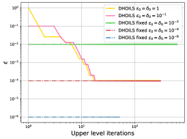
(a)

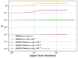
(b)

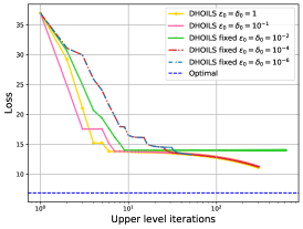
(c)

Figure 1: The values of $\epsilon$, $\delta$, and upper-level loss per upper-level iteration are shown under various settings of Algorithm 2 for solving the problem (42). The dynamic configurations in DHOILS manage to achieve the same range of the required accuracy $\epsilon$ regardless of the initial choice of $\epsilon_{0}$. Moreover, these configurations maintain or increase $\delta$ while progressively decreasing the loss.

Fig. 1 illustrates the determination of the necessary values for $\epsilon$ and $\delta$ in solving the problem (42) through the DHOILS algorithm. As demonstrated in Fig. 1(a), irrespective of the initial $\epsilon$ as the accuracy of the lower-level solver, Algorithm 2 dynamically reduces $\epsilon$, ultimately opting for accuracies around $10^{-4}$. Validation of the chosen lower-level solver accuracy in Algorithm 2 is confirmed in Fig. 1(c), revealing that with a fixed $\epsilon=10^{-2}$, the line search mechanism cannot identify a suitable step size, hindering progress after $9$ upper-level iterations. Conversely, in the case of adaptive accuracies and fixed accuracies with $\epsilon\leq 10^{-4}$, the loss consistently decreases towards the optimal value until the termination, which is triggered by reaching at maximum lower-level cost budget. The depiction of CG’s residual tolerance is presented in Fig. 1(b), wherein both dynamic scenarios of DHOILS maintain $\delta$ values at a steady level or elevate them during each upper-level iteration. This observation implies that the required accuracy for the inexact line search is adequately small within the confines of the error bound (2.1), facilitating the identification of a descent direction, even without obligatory reduction of $\delta$.

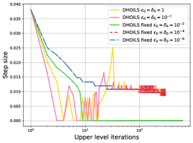
(a)

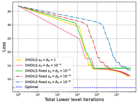
(b)

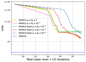
(c)

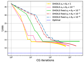
(d)

Figure 2: Performance and computational cost of the Algorithm 2 for solving the quadratic problem (42). The dynamic settings in DHOILS attain a similar range of upper-level step sizes, which closely resemble the step size chosen with high fixed accuracy. These settings result in a comparable loss value to the high fixed accuracy, all achieved at a lower computational cost.

Figure 2(a) illustrates how the inexact line search in Algorithm 3 finds a suitable step size in each upper-level iteration. In dynamic configurations, after several fluctuations in the initial upper-level iterations due to unsuccessful backtracking line searches while adjusting the accuracy $\epsilon$, both dynamic settings converge to the same range of step sizes that match the step size chosen in the fixed high-accuracy configurations of DHOILS. It should be mentioned that Fig. 2(a) shows that with a fixed low accuracy of $\epsilon=10^{-2}$, the line search mechanism fails, resulting in no positive step size being chosen after several iterations.

Considering the lower-level and CG iterations as the main computational costs, Figures 2(b), 2(c), and 2(d) demonstrate the computational advantages of the dynamic setting of Algorithm 2 compared to the fixed low and fixed high accuracies. By setting the low fixed accuracy to $\epsilon=10^{-2}$, both dynamic configurations reach the same loss as the fixed high accuracy of $\epsilon=10^{-4}$ while requiring fewer lower-level solver and CG iterations. However, using the higher fixed accuracy of $\epsilon=10^{-6}$ results in a higher loss than the dynamic configurations, as it exhausts the total budget of lower-level iterations. The importance of the dynamic approach in DHOILS is further amplified by highlighting that the suitable fixed accuracy is not known a priori; it may be too small and lead to failure as in the case of $\epsilon=10^{-2}$ or require significantly higher computational costs to make progress, as seen in the case of $\epsilon=10^{-6}$. In contrast, the dynamic configurations, regardless of the starting accuracy and step size, successfully proceed to solve the problem (42) with lower computational costs than a suitable fixed accuracy of $10^{-4}$.

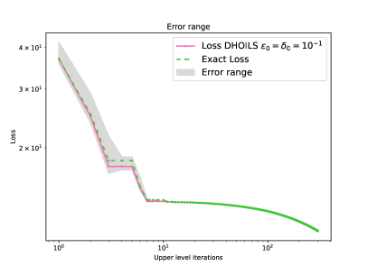
Figure 3: The range of error in upper-level function evaluation given error bounds (14a) and (14b), inexact loss given the approximated lower-level solution, and exact loss evaluation $f(\theta)$.

While in Fig. 1 and Fig. 2 we plot the upper-level loss computed using the estimated lower-level solution, it is also possible to compute the exact solution of the lower-level problem in the specific problem (42). This enables the calculation of the precise loss at each upper-level iteration. This ability allows us to verify both the sufficient decrease condition and the progress of the algorithm Algorithm 2. To facilitate this verification, we present the exact loss alongside the loss obtained using DHOILS with $\epsilon_{0}=\delta_{0}=10^{-1}$ in Fig. 3. Additionally, this figure visually represents the bounds for inexact loss evaluation, as defined by (14a) and (14b), wherein the area between these bounds encapsulates both exact and inexact loss values. Furthermore, as observed in Fig. 3, enhancing the accuracy of the lower-level solver leads to a narrower interval between the upper and lower bounds, thereby bringing the exact and inexact loss values closer. This phenomenon becomes more pronounced when the algorithm opts for accuracies around $\epsilon=10^{-4}$, suggesting that $\epsilon=10^{-4}$ is sufficiently high for this problem. Consolidating the outcomes depicted in Figures 1, 2, and 3, we can affirm the functionality, robustness concerning the choice of starting accuracy and step size, efficiency, and overall performance of the algorithm Algorithm 2 in solving the problem (42).

4.2 Multinomial logistic loss

In order to compare Algorithm 2 with HOAG [35] as a well-known gradient-based algorithm with inexact hypergradient, we replicate the multinomial logistic regression bilevel problem used in [35, 29] on the MNIST dataset. Similar to [35], we take the entire $60000$ training samples of MNIST and rescale them to $12\times 12$ pixels. Moreover, we utilize all $10000$ samples of the validation set for the upper-level problem. The bilevel problem corresponding to this model has the following form:

(43a) $$\min_{\theta\in\mathbb{R}^{d}}f(\theta) \coloneqq\sum_{i=1}^{N}\psi(\bar{b}_{i},\bar{a}_{i}^{T}\hat{x}(\theta)),$$

(43b) $$s.t.\quad\hat{x}(\theta) \coloneqq\arg\min_{x\in\mathbb{R}^{p\times q}}\sum_{j=1}^{M}\psi(b_{j},a_{j}^{T}x)+\frac{1}{2}\sum_{k=1}^{d}e^{\theta_{k}}x_{k}^{2},$$

Where $d=12\times 12\times 10=1440$ denotes the number of parameters, $\psi$ represents the multinomial logistic loss, and $a$ and $b$ correspond to the training images and labels. Similarly, $\bar{a}$ and $\bar{b}$ denote the validation images and labels in the upper-level problem. To solve this problem, we employ Algorithm 2 with various configurations, alongside HOAG using the heuristic adaptive step size with its default parameters. Moreover, HOAG begins with a starting accuracy of $\epsilon_{0}=\delta_{0}=10^{-1}$, as initialized in [35].

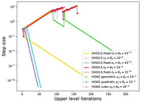
(a)

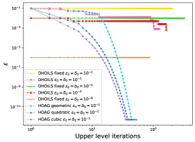
(b)

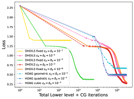
(c)

Figure 4: The values of $\epsilon$, $\delta$, and upper-level loss per total lower-level computational cost in the algorithms DHOILS and HOAG for solving the problem (43). It illustrates that the dynamic setting of DHOILS finds the same range of upper-level step size and the required accuracy for the solving the lower-level problem, while HOAG with the adaptive step size does not adjust the step size after a few iterations and exhibits a decreasing sequence for the accuracy $\epsilon$.

With a fixed total lower-level budget of $3\times 10^{5}$ iterations and $400$ upper-level iterations, Fig. 4 offers a comparison between HOAG and DHOILS in terms of upper-level step size, the accuracy of the lower-level solver, and loss. In HOAG, the initial step size was determined using the same strategy as outlined in [35], which is $\beta_{0}=\frac{\sqrt{d}}{\|z_{0}\|}$. During this experiment, all configurations of HOAG employing the adaptive step size strategy from [35] demonstrated the ability to adjust the step size and accuracy effectively, leading to initial progress and loss reduction in (43) within first $10$ upper-level iterations. However, HOAG’s adaptive step size mechanism encountered subsequent failures, causing the step size and accuracy for the lower-level solver to diminish to negligible values. As a result, the loss reduction stalled.

In contrast, regardless of the starting accuracy and using the same initial step size as HOAG, DHOILS consistently found an appropriate range for accuracy and upper-level step size, driving the loss to significantly lower values than those achieved by HOAG. While the lower fixed accuracy $\epsilon=10^{-1}$ became stuck and couldn’t make further progress after early iterations, a slightly higher fixed accuracy of $\epsilon=10^{-2}$ outperformed HOAG in terms of loss reduction, benefiting from the line search mechanism of Algorithm 2. However, it fell short of the dynamic setting’s accuracy. The high fixed accuracy of $\epsilon=10^{-6}$ demonstrated successful progression using DHOILS’s backtracking line search but required a higher computational cost for the lower-level solver compared to the dynamic setting. Furthermore, just as observed in the Quadratic problem (42), similar behaviors were noted for the $\delta$ parameter in DHOILS, either continuously increasing or maintaining stability across iterations.

In summation, DHOILS demonstrates improved adaptability and performance over HOAG by achieving lower loss values within the same lower-level computational budget. DHOILS achieved this by adaptively adjusting accuracy and step size, with this mechanism enhancing its robustness and efficiency.

4.3 Variational image denosing

4.3.1 Total variation denoising

In this part, we consider the smoothed version of the image-denoising model ROF [38] as implemented in [18]. Here, a bilevel problem is formulated to learn the smoothing and regularization parameters of total variation (TV) regularization. In contrast to the first numerical experiment in this section, access to the optimal hyperparameters is not possible a priori.

Similar to [18], we apply this model to $2D$ images and the training set is 25 images of the Kodak dataset resized to $96\times 96$ pixels, converted to grayscale, and Gaussian noise with $\mathcal{N}(0,\sigma^{2})$ with $\sigma=0.1$ is added. The bilevel problem we examine is as follows:

(44a) $$\min_{\theta}\frac{1}{2}\|\hat{x}(\theta)-\bar{x}\|^{2}$$

(44b) $$s.t.\quad\hat{x}(\theta)=\arg\min_{x}{\frac{1}{2}\|x-y\|^{2}}+e^{\theta_{1}}{\sum_{i,j}\sqrt{|\nabla x_{i}|^{2}+|\nabla x_{j}|^{2}+(e^{\theta_{2}})^{2}}}+\frac{e^{\theta_{3}}}{2}\|x\|^{2},$$

Here, $\nabla x_{i}$ and $\nabla x_{j}$ represent the forward differences in the horizontal and vertical directions, respectively. It is important to note that this problem satisfies all of the assumptions 2, 2, and 2. To initiate the process, we set $\theta_{0}=(-1,-1,0)$ and utilize Algorithm 2 along with the FISTA variant of DFO-LS with dynamic accuracy [18] to solve the problem (44). The DFO-LS with dynamic accuracy is a derivative-free bilevel algorithm that employs FISTA for solving the lower-level problem with an accuracy determined dynamically from the trust region radius in the derivative-free optimization algorithm for solving least-squares [13] in the upper-level problem. This algorithm serves as an efficient approach for solving bilevel problems and in particular for the problem (44). However, it should be noted that, as discussed in [16], in contrast with gradient-based algorithms, it may not scale well with the number of hyperparameters due to the nature of the derivative-free algorithm used for the upper-level problem. To maintain consistency with the first numerical example, we set a limit on the total number of lower-level iterations in this case.

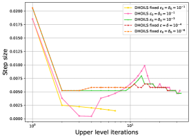
(a)

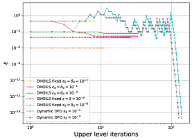
(b)

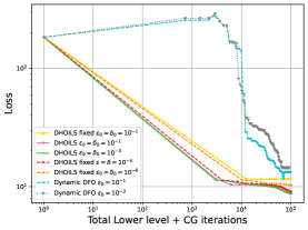
(c)

Figure 5: The values of $\epsilon$, $\delta$, and upper-level loss per total lower-level computational cost in the algorithms DHOILS and DFO-LS for solving the problem (44).

Illustrated in Fig. 5(a), DHOILS demonstrates how both dynamic and fixed high accuracy settings ensure the success of the line search mechanism, allowing the algorithm to adeptly adjust the step size. Consequently, DHOILS consistently arrives at the same range for the upper-level step size across both settings. Regarding the accuracy of the lower-level solver, the FISTA variant of DFO-LS initially selects a higher or equal value of $\epsilon$ compared to DHOILS, using the same starting accuracies. However, at a certain point, it begins to significantly decrease $\epsilon$. In terms of loss, with an equal total lower-level computational budget (assuming CG iterations of DFO-LS as zero), all variations of DHOILS surpass the performance of the FISTA variant of DFO-LS. While the insufficiently accurate fixed accuracy of $\epsilon=10^{-1}$ struggles to keep pace with the dynamic and high fixed accuracy settings of DHOILS, it experiences stagnation after a few upper-level iterations. Furthermore, it is important to note that DFO-LS does not utilize any hypergradient information, which could place it at a disadvantage when compared to gradient-based methods.

Now, to evaluate the effectiveness of the learned parameters obtained through solving (44) using DHOILS and dynamic DFO-LS, we apply these learned parameters to the lower-level total variation denoising problem for a test noisy image of size $720\times 720$. The learned parameters are chosen based on the results obtained from DHOILS with $\epsilon_{0}=\delta_{0}=10^{-1}$ and FISTA variant of dynamic DFO-LS with $\epsilon_{0}=\Delta_{0}=10^{-1}$ where $\Delta_{0}$ is the trust region radius in the first upper-level iteration.

(a)

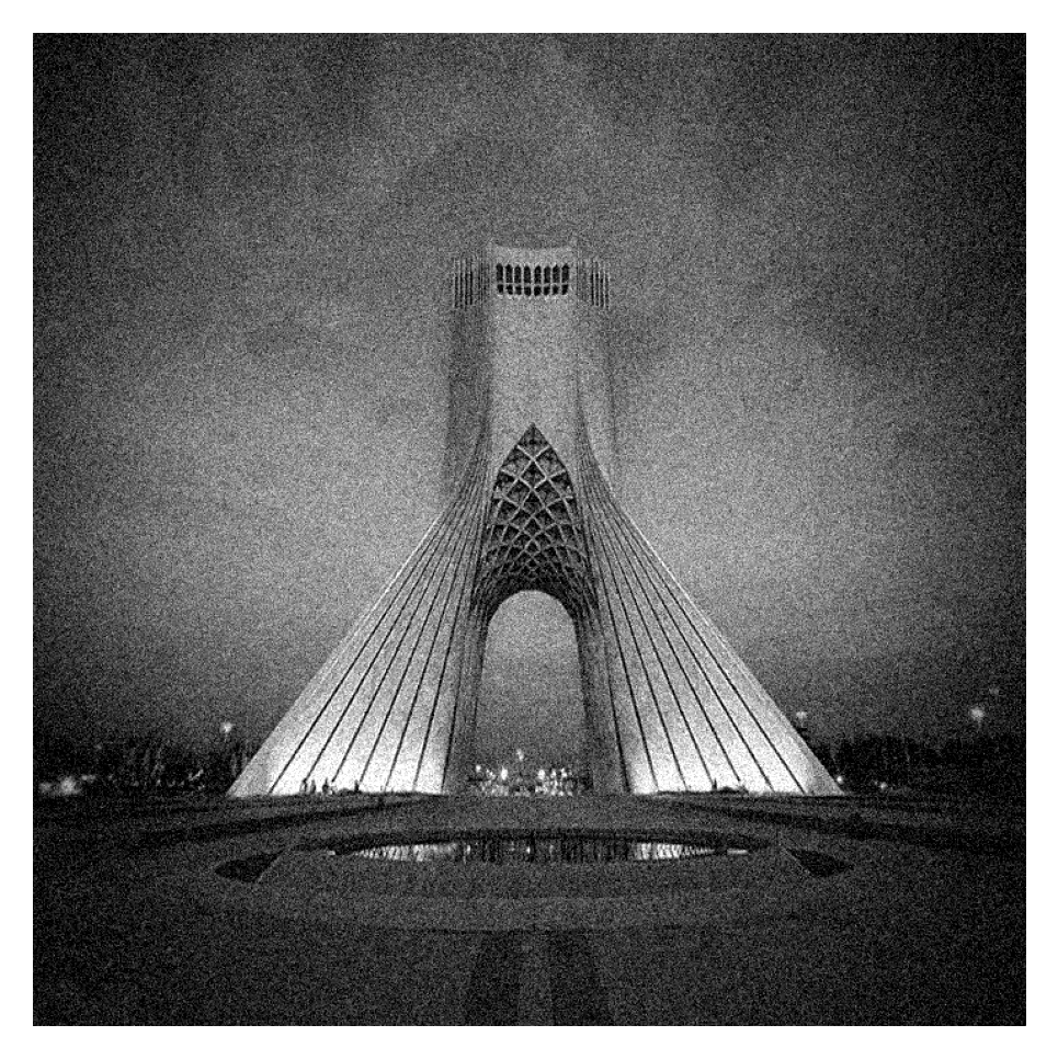
(b)

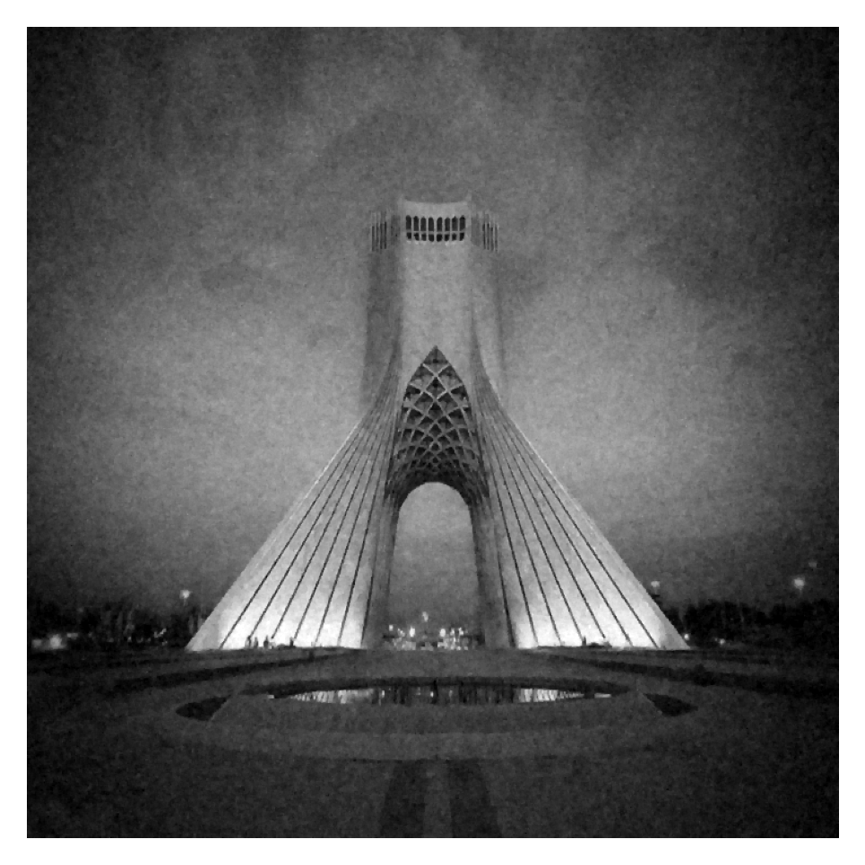
(c)

(d)

Figure 6: Total variation denoising with learned parameters.

Figure 6 shows the denoising results for both algorithms. The first row displays the original and noisy image, while the second row shows the denoised images obtained using DA and HOAG, respectively. Each denoised image is accompanied by its corresponding peak signal-to-noise ratio (PSNR) value. The learned hyperparameters using DHOILS result in higher PSNR values than DFO-LS learned hyperparameters on test images, which is consistent with the training results.

4.3.2 Field of experts denoising

In this part, we explore image denoising using a more data-adaptive regularizer known as the Field of Experts (FoE) approach. This approach was previously employed in a bilevel setting in [15] to learn the parameters of the regularizer in the variational setting. However, their choice of regularizer was non-convex and does not align with our assumptions. Therefore, we adopt the convex case, as described in [16], resulting in the following bilevel problem for each data point:

(45a) $$\min_{\theta}\frac{1}{2}\|\hat{x}(\theta)-\bar{x}\|^{2}$$

(45b) $$s.t.\quad\hat{x}(\theta)=\arg\min_{x}\left\{\frac{1}{2}\|x-y\|^{2}+e^{\theta_{0}}\sum_{k=1}^{K}e^{\theta_{k}}\|c_{k}\ast x\|_{\theta_{K+k}}+\frac{\mu}{2}\|x\|^{2}\right\},$$

where each $c_{k}$ is a $2D$ convolution kernel, and we added the term $\frac{\mu}{2}\|\cdot\|^{2}$ to have a $\mu$-strongly convex lower-level objective function. We set $K=30$ and take each $c_{k}$ as a $7\times 7$ kernel with elements $[\theta_{2K+49(k-1)+1},\dots,\theta_{2K+49k}]$. We also set $\mu=10^{-8}$ but it can also be part of the learnable parameters. Also, $\|x\|_{\nu}=\sum_{j=1}^{N}\sqrt{x_{j}^{2}+\nu^{2}}$ represents the smoothed $1$-norm with smoothing parameter $\nu$ for any $x\in\mathbb{R}^{N}$. So, this problem has $1531$ hyperparameters that we represent by $\theta$. We initialize the kernels by drawing randomly from a Gaussian distribution with mean $0$ and standard deviation $1$, and we set the initial weights to $e^{-3}$. During training, similar to TV denoising, we use 25 images from the Kodak dataset and rescale them to $96\times 96$ pixels, converting them to grayscale. Additionally, we add Gaussian noise with $\mathcal{N}(0,\sigma^{2})$, where $\sigma=0.1$, to the ground truth images.

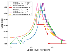
(a)

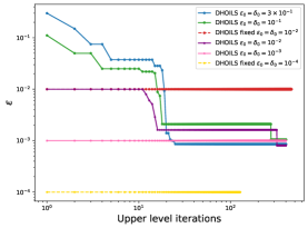
(b)

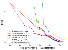
(c)

Figure 7: Investigating the impact of DHOILS configurations on chosen step size, the accuracy of the lower-level solver, and loss at each lower-level computation unit with varied $\epsilon_{0}$ and $\delta_{0}$ for solving the problem (45).

As seen in Fig. 7(a), the robustness of Algorithm 2 becomes evident in its ability to find a suitable step size. When initiated with low accuracies such as $\epsilon=3\times 10^{-1}$ and $10^{-1}$, the line search encounters early failures. However, by dynamically adjusting the accuracy within the framework of Algorithm 2, the algorithm regains momentum, ultimately selecting the same range of accuracies as both the dynamic and fixed high accuracy settings in DHOILS. Akin to the patterns observed in previous numerical experiments, the challenge of selecting a suitable step size emerges with the low fixed accuracy setting, causing it to stagnate after several upper-level iterations. This consistent behavior also extends to the selection of the required accuracy for the lower-level solver, as showcased in Fig. 7(b).

For the DHOILS variant starting with the lowest accuracy, it requires a slightly greater number of lower-level computations to advance compared to the dynamic cases with higher starting accuracies. This behavior is attributed to the initial need for more lower-level iterations due to the line search mechanism’s initial failures during accuracy adjustments. Nevertheless, all dynamic instances of DHOILS effectively make notable progress in solving problem (45) with a reduced computational burden when compared to high fixed accuracy settings. These dynamic instances demonstrate the capacity to adaptively determine both accuracy and step size, enhancing their overall efficiency.

Noting the importance of the problem (45) as a large-scale and data-adaptive problem, we evaluated the learned parameters using Algorithm 2 on a noisy test image of size $720\times 720$ pixels with Gaussian noise with $\sigma=0.1$, as depicted in Fig. 8(a) and Fig. 8(b), respectively. The quality of the learned parameters and, consequently, the denoised image obtained through Algorithm 2 are illustrated in Fig. 8(c), where the denoised image achieved a PSNR of $28.68$.

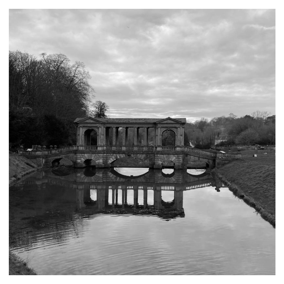
(a)

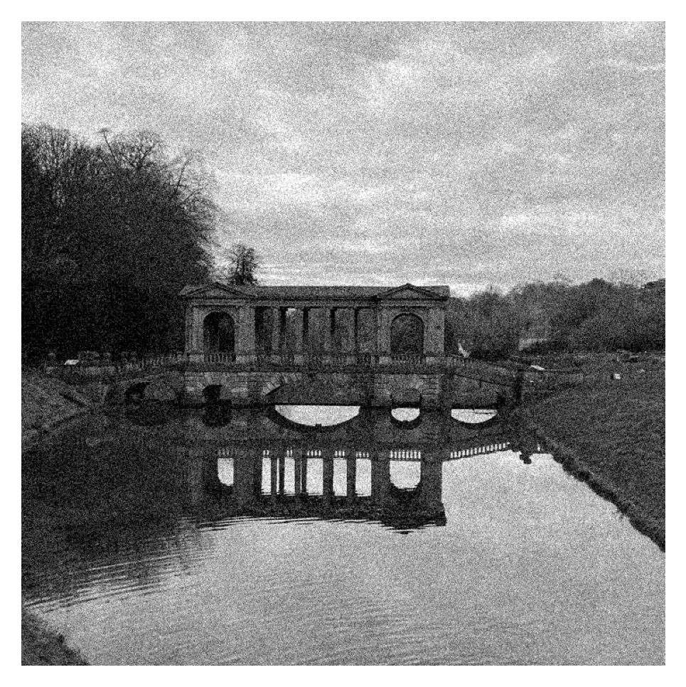
(b)

(c)

Figure 8: Field of experts denoising with learned parameters utilizing Algorithm 2.

5 Conclusion

This study has introduced a comprehensive framework for bilevel optimization with strongly convex lower-level problems, inexact line search method based on adaptive control of the accuracy of lower-level solver and hypergradient calculations, that ensures the approximate hypergradient serves as a descent direction, coupled with a provably convergent inexact line search strategy that utilizes both approximate function evaluations and the approximate hypergradient. Accompanying this framework is an algorithm that adaptively determines the required accuracy for the inexact line search. Our numerical results underscore the superiority of this framework over state-of-the-art methods for bilevel learning across a range of problems. Importantly, it demonstrates remarkable robustness in the face of initial accuracy and starting step size choices, alleviating the need for tuning these algorithm parameters specifically for each problem. Future work on this method will examine a worst-case complexity analysis and encompass potential future extensions, including stochastic variants of this framework.

References

- [1] B. Amos, L. Xu, and J. Z. Kolter, Input convex neural networks, 2017, https://arxiv.org/abs/1609.07152.
- [2] C. Arndt, Regularization theory of the analytic deep prior approach, Inverse Problems, 38 (2022), p. 115005.
- [3] A. Beck, First-Order Methods in Optimization, Society for Industrial and Applied Mathematics, Philadelphia, PA, 2017.
- [4] A. Beck and M. Teboulle, A fast iterative shrinkage-thresholding algorithm for linear inverse problems, SIAM Journal on Imaging Sciences, 2 (2009), pp. 183–202.
- [5] Y. Bengio, Gradient-based optimization of hyperparameters, Neural Computation, 12 (2000), pp. 1889–1900.
- [6] A. S. Berahas, L. Cao, and K. Scheinberg, Global convergence rate analysis of a generic line search algorithm with noise, SIAM Journal on Optimization, 31 (2021), pp. 1489–1518, https://doi.org/10.1137/19M1291832.
- [7] J. Bergstra and Y. Bengio, Random search for hyper-parameter optimization, J. Mach. Learn. Res., 13 (2012), p. 281–305.
- [8] Q. Bertrand, Q. Klopfenstein, M. Massias, M. Blondel, S. Vaiter, A. Gramfort, and J. Salmon, Implicit differentiation for fast hyperparameter selection in non-smooth convex learning, 2022, https://arxiv.org/abs/2105.01637.
- [9] L. Bogensperger, A. Chambolle, and T. Pock, Convergence of a piggyback-style method for the differentiation of solutions of standard saddle-point problems, SIAM Journal on Mathematics of Data Science, 4 (2022), pp. 1003–1030.
- [10] J. Bolte, E. Pauwels, and S. Vaiter, Automatic differentiation of nonsmooth iterative algorithms, in Advances in Neural Information Processing Systems, S. Koyejo, S. Mohamed, A. Agarwal, D. Belgrave, K. Cho, and A. Oh, eds., vol. 35, Curran Associates, Inc., 2022, pp. 26404–26417.
- [11] J. Bolte, E. Pauwels, and S. Vaiter, One-step differentiation of iterative algorithms, 2023, https://arxiv.org/abs/2305.13768.
- [12] C. Cartis, J. Fiala, B. Marteau, and L. Roberts, Improving the flexibility and robustness of model-based derivative-free optimization solvers, 2018, https://arxiv.org/abs/1804.00154.
- [13] C. Cartis and L. Roberts, A derivative-free gauss-newton method, 2017, https://arxiv.org/abs/1710.11005.
- [14] A. Chambolle and T. Pock, An introduction to continuous optimization for imaging, Acta Numerica, 25 (2016), pp. 161–319.
- [15] Y. Chen, R. Ranftl, and T. Pock, Insights into analysis operator learning: From patch-based sparse models to higher order MRFs, IEEE Transactions on Image Processing, 23 (2014), pp. 1060–1072.
- [16] C. Crockett and J. A. Fessler, Bilevel methods for image reconstruction, Foundations and Trends® in Signal Processing, 15 (2022), pp. 121–289.
- [17] S. Dittmer, T. Kluth, P. Maass, and D. O. Baguer, Regularization by architecture: A deep prior approach for inverse problems, Journal of Mathematical Imaging and Vision, 62 (2019), pp. 456–470.
- [18] M. J. Ehrhardt and L. Roberts, Inexact derivative-free optimization for bilevel learning, 2020, https://arxiv.org/abs/2006.12674.
- [19] M. J. Ehrhardt and L. Roberts, Analyzing inexact hypergradients for bilevel learning, 2023.
- [20] P. I. Frazier, A tutorial on bayesian optimization, 2018, https://arxiv.org/abs/1807.02811.
- [21] A. Goujon, S. Neumayer, P. Bohra, S. Ducotterd, and M. Unser, A neural-network-based convex regularizer for image reconstruction, 2022, https://arxiv.org/abs/2211.12461.
- [22] R. Grazzi, M. Pontil, and S. Salzo, Convergence properties of stochastic hypergradients, 2021, https://arxiv.org/abs/2011.07122.
- [23] A. Griewank and C. Faure, Piggyback differentiation and optimization, in Large-Scale PDE-Constrained Optimization, L. T. Biegler, M. Heinkenschloss, O. Ghattas, and B. van Bloemen Waanders, eds., Berlin, Heidelberg, 2003, Springer Berlin Heidelberg, pp. 148–164.
- [24] P. Khanduri, S. Zeng, M. Hong, H.-T. Wai, Z. Wang, and Z. Yang, A near-optimal algorithm for stochastic bilevel optimization via double-momentum, 2021, https://arxiv.org/abs/2102.07367.
- [25] K. Kunisch and T. Pock, A bilevel optimization approach for parameter learning in variational models, SIAM J. Imaging Sci., 6 (2013), pp. 938–983.
- [26] J. Li, B. Gu, and H. Huang, A fully single loop algorithm for bilevel optimization without hessian inverse, Proceedings of the AAAI Conference on Artificial Intelligence, 36 (2022), pp. 7426–7434.
- [27] D. C. LIU and J. NOCEDAL, On the limited memory BFGS method for large scale optimization, Math. Programming, 45 (1989), pp. 503–528.
- [28] J. Lorraine and D. Duvenaud, Stochastic hyperparameter optimization through hypernetworks, 2018, https://arxiv.org/abs/1802.09419.
- [29] D. Maclaurin, D. Duvenaud, and R. P. Adams, Gradient-based hyperparameter optimization through reversible learning, 2015, https://arxiv.org/abs/1502.03492.
- [30] S. Mehmood and P. Ochs, Automatic differentiation of some first-order methods in parametric optimization, in Proceedings of the Twenty Third International Conference on Artificial Intelligence and Statistics, S. Chiappa and R. Calandra, eds., vol. 108 of Proceedings of Machine Learning Research, PMLR, 26–28 Aug 2020, pp. 1584–1594.
- [31] S. Mukherjee, S. Dittmer, Z. Shumaylov, S. Lunz, O. Öktem, and C.-B. Schönlieb, Learned convex regularizers for inverse problems, 2020.
- [32] Y. Nesterov, Lectures on Convex Optimization, Springer Publishing Company, Incorporated, 2nd ed., 2018.
- [33] J. Nocedal and S. J. Wright, Numerical Optimization, Springer Series in Operations Research and Financial Engineering, Springer, New York, 2 ed., 2006.
- [34] P. Ochs, R. Ranftl, T. Brox, and T. Pock, Techniques for gradient based bilevel optimization with nonsmooth lower level problems, 2016.
- [35] F. Pedregosa, Hyperparameter optimization with approximate gradient, 2016, https://arxiv.org/abs/1602.02355.
- [36] Z. Ramzi, F. Mannel, S. Bai, J.-L. Starck, P. Ciuciu, and T. Moreau, Shine: Sharing the inverse estimate from the forward pass for bi-level optimization and implicit models, 2023, https://arxiv.org/abs/2106.00553.
- [37] J. C. D. l. Reyes and D. Villacís, Bilevel Optimization Methods in Imaging, Springer International Publishing, 2023, pp. 909–941.
- [38] L. I. Rudin, S. Osher, and E. Fatemi, Nonlinear total variation based noise removal algorithms, Physica D: Nonlinear Phenomena, 60 (1992), pp. 259–268.
- [39] F. Sherry, M. Benning, J. C. D. los Reyes, M. J. Graves, G. Maierhofer, G. Williams, C.-B. Schönlieb, and M. J. Ehrhardt, Learning the sampling pattern for mri, 2020, https://arxiv.org/abs/1906.08754.
- [40] H.-J. M. Shi, Y. Xie, R. Byrd, and J. Nocedal, A noise-tolerant quasi-newton algorithm for unconstrained optimization, SIAM Journal on Optimization, 32 (2022), pp. 29–55, https://doi.org/10.1137/20M1373190.
- [41] H. Yang, L. Luo, C. J. Li, and M. I. Jordan, Accelerating inexact hypergradient descent for bilevel optimization, 2023, https://arxiv.org/abs/2307.00126.
- [42] J. Yang, K. Ji, and Y. Liang, Provably faster algorithms for bilevel optimization, 2021, https://arxiv.org/abs/2106.04692.
- [43] N. Zucchet and J. Sacramento, Beyond backpropagation: Bilevel optimization through implicit differentiation and equilibrium propagation, Neural Computation, 34 (2022), pp. 2309–2346.