The Distribution of Strike Size:Empirical Evidence from Europe and North America in the 19th and 20th Centuries

Abstract

We study the distribution of strike size, which we measure as lost person days, for a long period in several countries of Europe and America. When we consider the full samples, the mixtures of two or three lognormals arise as very convenient models. When restricting to the upper tails, the Pareto power law becomes almost indistinguishable of the truncated lognormal.

1 Introduction

Ref. [42] highlighted that the sizes above a threshold (however measured) for physical, biological or economic phenomena (e.g., cities and firms) are well described by a power law distribution. This distribution, as well as the mechanisms that give rise to it, have also been explored in the literature examining the size of conflicts [55, 56, 16, 19, 25, 31]. More recently, interest has also turned to the distribution of strike size [8, 9, 14], a much less violent form of conflict, but one that can have substantial economic consequences. Interestingly, the size of firms and unions have both been found to be described by power law distributions (e.g., among many others, [38, 3, 51]) and strikes are embedded in these firms and unions.

The presence of a power law distribution in strike size has a few important implications. As emphasized by [14], the total costs of strikes to the economy will be created by a small percentage of strikes, not unlike Pareto’s rule where 20 percent of the population hold 80 percent of the wealth. Another important implication of power law distributions is that they may give rise to self-organizing systems, in which a system’s organization is determined by behavior of individual agents acting in response to one another [4, 42, 24]. If strikes are self-organizing then that suggests that they are not likely to be affected by legislation and interventions by third parties (i.e., factors outside the “system”) and might also give rise to strike waves as they spread through sectors or regions as more persons join them. Consequently, understanding the distribution of strike size is quite important from the perspective of many economic stakeholders, e.g., legislators, firms and union members. In addition, understanding the distribution of strike size could also provide insights into the potential models that could describe strike dynamics [8, 14].

However, while the upper tail of the distribution could be fit by the power law distribution (e.g., [8, 9, 14]), the nature of the distribution below the upper tail is still not understood. In addition, it is often difficult to distinguish the power law from other alternative distributions in the upper tail, so that alternative distributions could also be plausible fits [18]. Moreover, is there a distribution that could fit the whole range of the data, and not focus on the upper or lower tail? Recently, papers have also begun exploring alternatives to the power law distribution in many empirical settings and also considering the fit below the upper tail (e.g., the size of cities [43, 12, 61, 53], the size of business firms [62]).

We study the size distribution of strikes using micro data on strikes from a few European countries (France and the Netherlands) as well as Canada and the United States. Our data spans a long time period, covering strikes before World War II as well as after the War. Using data from such a long time period means that we can compare the estimates across countries during similar periods as well different periods and so infer whether the distribution of strikes is generated by a mechanism that is common to all countries and all time periods. In other words, is the distribution of strike size relatively stable across time and countries. We measure strike size with the number of person days lost to a strike (number of workers on strike multiplied by the duration of strike). We consider distributions such as the lognormal and power law as well as mixtures of lognormal distributions and truncated lognormal distributions. We obtain our estimates using maximum likelihood estimators and to evaluate the fit of the distributions we consider standard statistical tests as well as using information criteria to select the most appropriate distribution. Finally, we also discuss some of the plausible generating mechanisms for the distributions that we consider, showing how they arise from the stationary solutions of Fokker-Planck equations.

This paper makes the following contributions to the literature:

• We show that the distribution of lost-person-days measure of strike size using data in the upper tail and below it follows a mixture of two or three lognormals.

• When restricting to the upper tail, according to the procedure of [19], it becomes difficult to distinguish between a Pareto power law and a (upper-tail) truncated lognormal.

• The upper tail is plausibly described by a power law, although other models can parameterize it as good as the former.

• We formulate stochastic models that generate the lognormal mixtures as well as the other distributions we consider.

The rest of the paper is organized as follows. The next section of the paper presents the methodology we follow. We describe our data in Section 3 and present a discussion of our findings in Section 4. In Section 5 we provide a summary of our findings and their implications.

2 Methods and Generating Mechanisms

In this section we will introduce the distributions used throughout the paper. We let $x$ denote our measure of strike size, lost-person-days.

The first distribution we consider for lost-person-days, $x>0,$ is the stretched exponential (STEXP) distribution

$$f_{\mathrm{STEXP}}(x;\gamma,\eta)=\frac{\gamma}{\eta}\left(\frac{x}{\eta}\right)^{\gamma-1}\exp\left(-\left(\frac{x}{\eta}\right)^{\gamma}\right)$$

where $\gamma$ is a shape parameter, which is such that $0<\gamma<1$, and $\eta>0$ is a scale parameter. Stretched exponential distributions have often been found to fit skewed and heavy-tailed data [45, 40].

The second distribution in our study is the well-known lognormal distribution

$$f_{\mathrm{LN}}(x;\mu,\sigma)=\frac{1}{\sqrt{2\pi}\sigma x}\exp\left(-\frac{(\ln(x)-\mu)^{2}}{2\sigma^{2}}\right)$$

where $\mu$ is the mean of $\ln(x)$ and $\sigma>0$ is its standard deviation according to this distribution. Lognormal distributions have been found to fit many economic and physical phenomena with heavy tails [48].

While lognormal distributions are skewed and can have heavy tails, they might not be able to capture the skewness and kurtosis of some data. An alternative that might be better able to do so is a mixture of distributions, which include several lognormal distributions [36, 47]. Mixtures of $m\geq 2$ lognormal distributions have the density

$$f_{m\mathrm{LN}}(x;\mu_{1},\sigma_{1},\ldots,\mu_{m},\sigma_{m},p_{1},\ldots,p_{m-1})=\sum_{j=1}^{m-1}p_{j}f_{\mathrm{LN}}(x;\mu_{j},\sigma_{j})+\left(1-\sum_{j=1}^{m-1}p_{j}\right)f_{\mathrm{LN}}(x;\mu_{m},\sigma_{m})$$

where $\mu_{1},\ldots,\mu_{m}>0$, $\sigma_{1},\ldots,\sigma_{m}>0$, and $0\leq p_{1},\ldots,p_{m-1},p_{1}+\dots+p_{m-1}\leq 1$. In this paper, we will consider 2-mixtures ($m=2$) and 3-mixtures ($m=3$), which we denote as 2LN and 3LN.

Another alternative for the distribution of strike size, which has been considered in the earlier literature [8, 9, 14] is the power law distribution (or Pareto distribution):

$$f_{\mathrm{P}}(x;\alpha,x_{\mathrm{min}})=\frac{\alpha-1}{x_{\mathrm{min}}}\left(\frac{x}{x_{\mathrm{min}}}\right)^{-\alpha}$$

where $\alpha$ is the power law exponent and $x_{\mathrm{min}},$ which is such that $x\geq$ $x_{\mathrm{min}}>0$, is the lower bound on power law behavior. Unlike the stretched exponential, lognormal and mixtures of lognormal distributions we consider, which take $x>0,$ the support of the power law distribution is $x\geq x_{\mathrm{min}}$, so it only considers the upper tail of the data.

However, one issue that has been highlighted in the research literature is that it can be difficult to distinguish a power law distribution with the upper tail of other heavy tailed distributions [18]. This means that there could be other distributions that are a plausible fit to the upper tail of the data. An implication of this observation is that an empirical analysis should also consider the fits of alternative distributions to the upper tail [18]. Consequently, we also consider a truncated lognormal

$$f_{\mathrm{LNt}}(x;\mu,\sigma,x_{\mathrm{min}})=\frac{f_{\mathrm{LN}}(x;\mu,\sigma)}{1-\mathrm{cdf}_{\mathrm{LN}}(x_{\mathrm{min}};\mu,\sigma)}$$

where $x_{\mathrm{min}}$ is the minimum value of the variable of the range considered ($x\in[x_{\mathrm{min}},\infty)$) and

$$\mathrm{cdf}_{\mathrm{LN}}(x;\mu,\sigma)=\frac{1}{2}+\frac{1}{2}\mathrm{erf}\left(\frac{\ln(x)-\mu}{\sqrt{2}\sigma}\right)$$

is the cumulative distribution function (CDF) of the lognormal distribution ($\mathrm{erf}$ is the error function associated to the standard normal distribution). The truncated lognormal distribution has been considered as an alternative to a power law distribution in the upper tail of wealth [13].

We estimate all these distributions with maximum likelihood (ML) estimation.

We assess the fit using the log-rank/corank plots to value the fit visually. As is well known, the tails of a power law distribution should produce a straight line in a log-rank/corank plot. We also assess the fit of the distributions to the data with goodness of fit tests. Namely, we use the Kolmogorov–Smirnov (KS), Anderson–Darling (AD) and Cramér–von Mises (CM) tests.

The visual and statistical assessments of the models allow us to discern the distributions that are a good fit to the data. However, the question remains which of the distributions is the best fit or most appropriate if the tests for fit indicate that they are plausible alternatives. Ref. [2] advised that theory and economic intuition should guide model selection. However, if they are unable to provide guidance, model selection can be undertaken using information criteria.

We use three well-known information criteria in order to select the most preferred model from those we consider. They are:

• The Akaike Information Criterion (AIC) [1, 10, 11], defined as

  $$AIC=2k-2\ln L^{*}$$

  where $k$ is the number of parameters of the distribution and $\ln L^{*}$ is the corresponding (maximum) log-likelihood. The minimum value of AIC corresponds (asymptotically) to the minimum value of the Kullback–Leibler divergence, so a model with the lowest AIC is selected from among the competitors.

• The Bayesian or Schwarz Information Criterion (BIC) [10, 11, 59], defined as

  $$BIC=k\ln(n)-2\ln L^{*}$$

  where $k$ is the number of parameters of the distribution, $n$ the sample size and $\ln L^{*}$ is as before. The BIC penalizes more heavily the number of parameters used than does the AIC. The model with the lowest BIC is selected according to this criterion.

• The Hannan–Quinn Information Criterion (HQC) [10, 11, 37], defined as

  $$HQC=2k\ln(\ln(n))-2\ln L^{\ast}$$

  where $k$ is the number of parameters of the distribution, $n$ the sample size and $\ln L^{\ast}$ is as before. The HQC implements an intermediate penalization of the number of parameters when compared to the AIC and BIC. The model with the lowest HQC is selected according to this criterion.

The information criteria aid us in selecting the most appropriate distribution for the data.

A more difficult question is sorting among the mechanisms that create the distribution of strike size. Some earlier work, [14], points to two mechanisms that could create a power law distribution in the upper tail of the distribution of strike size. First, the safety valve hypothesis, where dissatisfaction and conflict builds up in a workplace reaches a critical point and is then released as a strike. This model is like a forest fire model, which has also been applied to study the spread of conflict [16, 8]. Second, the joint costs model, where the incidence and duration of strikes is inversely related to the costs of striking. Both of these mechanisms would create a power law distribution in the upper tail. However, it is not clear whether these mechanisms would be consistent with the other distributions, e.g., stretched exponential, the lognormal, truncated lognormal or mixture of lognormals, that we consider. To obtain these alternative distributions we need a more general dynamic model.

In order to achieve this task, let us denote first the natural logarithm of the strike size variable by $y=\ln(x)$ in what follows, and then $y\in(-\infty,\infty)$. Then the stretched exponential becomes the “exponential stretched exponential”:

$$f_{\mathrm{ESTEXP}}(y;\gamma,\eta)=\gamma\exp\left(-\left(\frac{\mathrm{e}^{y}}{\eta}\right)^{\gamma}\right)\left(\frac{\mathrm{e}^{y}}{\eta}\right)^{\gamma}$$

where, as before, $0<\gamma<1$ and $\eta>0$. With the previous change of variable, the lognormal becomes a normal distribution (N), the mixtures 2LN and 3LN become, in an obvious notation, the mixtures 2N and 3N, the power law or Pareto distribution becomes an exponential distribution like

$$f_{\mathrm{EXP}}(y;\alpha,y_{\mathrm{min}})=(\alpha-1)\exp\left(-(\alpha-1)(y-y_{\mathrm{min}})\right)$$

where $y_{\mathrm{min}}=\ln(x_{\mathrm{min}})$ and $y_{\mathrm{min}}\leq y$. The truncated lognormal becomes, likewise, a truncated normal:

$$f_{\mathrm{Nt}}(y;\mu,\sigma,y_{\mathrm{min}})=\frac{f_{\mathrm{N}}(y;\mu,\sigma)}{1-\mathrm{cdf}_{\mathrm{N}}(y_{\mathrm{min}};\mu,\sigma)}$$

where, obviously, $y_{\mathrm{min}}$ is as in the previous exponential distribution with $y_{\mathrm{min}}\leq y$, and

$$f_{\mathrm{N}}(y;\mu,\sigma)=\frac{1}{\sqrt{2\pi}\sigma}\exp\left(-\frac{(y-\mu)^{2}}{2\sigma^{2}}\right)$$

$$\mathrm{cdf}_{\mathrm{N}}(y;\mu,\sigma)=\frac{1}{2}+\frac{1}{2}\mathrm{erf}\left(\frac{y-\mu}{\sqrt{2}\sigma}\right)$$

being now $\mu\in(-\infty,\infty)$.

We consider stochastic models whose stationary density functions are the distributions just described. Let $y_{t}$ denote a random variable, which in principle can depend on time, whose evolution or dynamics is governed by the Itô differential equation (see, e.g., [50, 30])

$$dy_{t}=b(y_{t},t)dt+\sqrt{a(y_{t},t)}dB_{t}$$ (1)

where $B_{t}$ is a standard Brownian motion (Wiener process) (see, e.g., [39, 44] and references therein). The quantity $a(y_{t},t)$ corresponds to the diffusion term, and $b(y_{t},t)$ to the drift term. This process can be associated to the forward Kolmogorov equation or Fokker-Planck equation for the time-dependent probability density function (conditional on the initial data) $f(y,t)$ (see also [28, 29]):

$$\frac{\partial f(y,t)}{\partial t}=-\frac{\partial}{\partial y}(b(y,t)f(y,t))+\frac{1}{2}\frac{\partial^{2}}{\partial y^{2}}(a(y,t)f(y,t)).$$

Like most of the literature (see, e.g., [23, 33, 35, 34, 49]), we work with stationary probability density functions, so that for different choices of (time-independent) $b(y)$ and $a(y)$, the Fokker–Planck equation can be solved and produce the distributions we consider [50, 21, 23, 27, 20, 35] For example, the “exponential stretched exponential” is a stationary solution of the Fokker–Planck equation with the choice $a(y)=\sigma^{2}$, where $\sigma>0$ is a constant, and

$$b(y)=-\frac{\gamma\sigma^{2}}{2}\left(\left(\frac{\mathrm{e}^{y}}{\eta}\right)^{\gamma}-1\right)$$

Stretched exponential distributions can be generated as well by multiplicative processes with limiting behavior determined by the application of extreme deviations theory [45, 26]. The recent work [15] discussed how extreme deviations theory applied to a proportionate growth model, which is the deterministic version of the Brownian motion in equation (1), will generate a stretched exponential distribution. Likewise, the normal distribution can be obtained as a stationary solution to Fokker–Planck equation by assuming the diffusion term is given as well by a constant [63, 41, 67] $a(y)=\sigma^{2}$ and $b(y)=-\frac{1}{2}(y-\mu)$, exhibiting mean reversion. The exponential distribution can also be obtained as a stationary solution to the Fokker–Planck equation with drift and diffusion terms given by $a(y)=\sigma^{2}$, ${\displaystyle b(y)=-\frac{1}{2}(\alpha-1)\sigma^{2}}$. We can also obtain the truncated normal distribution as a stationary solution to the Fokker–Planck equation, with drift and diffusion terms $a(y)=\sigma^{2}$, ${\displaystyle b(y)=-\frac{1}{2}(y-\mu)}$. This is similar to our solution for the normal equation distribution pointed out earlier, except that now the support of the distribution is $[y_{\mathrm{min}},\infty)$.

We can also obtain mixtures of normal distributions, our (exponentiated) models $f_{\mathrm{2N}}$, $f_{\mathrm{3N}}$ (mixtures of two or three normals, respectively) as stationary solutions to the Fokker–Planck equations and formulate stochastic equations for the strike processes. We first consider $f_{\mathrm{2N}}$, a mixture of two normal distributions, given by

$$f_{\mathrm{2N}}(y;\mu_{1},\sigma_{1},\mu_{2},\sigma_{2},p_{1})=p_{1}f_{\mathrm{N}}(y;\mu_{1},\sigma_{1})+(1-p_{1})f_{\mathrm{N}}(y;\mu_{2},\sigma_{2})$$

where $0\leq p_{1},1-p_{1}\leq 1$. We will denote for simplicity the posterior probabilities (see, e.g., [47])

$$\tau_{1}(y)=p_{1}f_{\mathrm{N}}(y;\mu_{1},\sigma_{1})/f_{\mathrm{2N}}(y;\mu_{1},\sigma_{1},\mu_{2},\sigma_{2},p_{1})$$

$$\tau_{2}(y)=(1-p_{1})f_{\mathrm{N}}(y;\mu_{2},\sigma_{2})/f_{\mathrm{2N}}(y;\mu_{1},\sigma_{1},\mu_{2},\sigma_{2},p_{1})$$

Then, let the diffusion and drift terms be defined by $a(y)=\sigma^{2}$, and

$$b(y)=-\frac{\sigma^{2}}{2\sigma_{1}^{2}}\tau_{1}(y)(y-\mu_{1})-\frac{\sigma^{2}}{2\sigma_{2}^{2}}\tau_{2}(y)(y-\mu_{2})$$

so that we obtain that the $f_{\mathrm{2N}}$ above is a stationary solution of the corresponding Fokker–Planck equation. This is a novel, as far as we know, generalization of the results of [63, 41, 67], where the relevant quantities can be functions of $y$ with definite sign. For the $f_{\mathrm{3N}}$, that is, a mixture of three normal distributions, it is completely analogous to the case of 2N. The 3N can be given by

$$f_{\mathrm{3N}}(y;\mu_{1},\sigma_{1},\mu_{2},\sigma_{2},\mu_{3},\sigma_{3},p_{1},p_{2})=p_{1}f_{\mathrm{N}}(y;\mu_{1},\sigma_{1})+p_{2}f_{\mathrm{N}}(y;\mu_{2},\sigma_{2})+(1-p_{1}-p_{2})f_{\mathrm{N}}(y;\mu_{3},\sigma_{3})$$

where $0\leq p_{1},p_{2},1-p_{1}-p_{2}\leq 1$. We define in this case the corresponding posterior probabilities

$$\tau_{1}(y)=p_{1}f_{\mathrm{N}}(y;\mu_{1},\sigma_{1})/f_{\mathrm{3N}}(y;\mu_{1},\sigma_{1},\mu_{2},\sigma_{2},\mu_{3},\sigma_{3},p_{1},p_{2})$$

$$\tau_{2}(y)=p_{2}f_{\mathrm{N}}(y;\mu_{2},\sigma_{2})/f_{\mathrm{3N}}(y;\mu_{1},\sigma_{1},\mu_{2},\sigma_{2},\mu_{3},\sigma_{3},p_{1},p_{2})$$

$$\tau_{3}(y)=(1-p_{1}-p_{2})f_{\mathrm{N}}(y;\mu_{3},\sigma_{3})/f_{\mathrm{3N}}(y;\mu_{1},\sigma_{1},\mu_{2},\sigma_{2},\mu_{3},\sigma_{3},p_{1},p_{2})$$

and the diffusion and drift terms defined by $a(y)=\sigma^{2}$,

$$b(y)=-\frac{\sigma^{2}}{2\sigma_{1}^{2}}\tau_{1}(y)(y-\mu_{1})-\frac{\sigma^{2}}{2\sigma_{2}^{2}}\tau_{2}(y)(y-\mu_{2})-\frac{\sigma^{2}}{2\sigma_{3}^{2}}\tau_{3}(y)(y-\mu_{3})$$

we obtain that the $f_{\mathrm{3N}}$ above is a stationary solution of the corresponding Fokker–Planck equation.

The Fokker–Planck equations are the continuous time counterparts to the dynamics that arise in kinetic models. These kinetic models have been increasingly used to study socioeconomic and human behavior [33, 35, 34, 20, 27]. These models may also be applicable when considering processes generating strikes, which arise during collective bargaining, i.e., the interactions between the unions, the bargaining agent for workers, with management. In particular, there are individual agents, which are comprised of firm and union representatives who form a bargaining pair. The collective bargaining that occurs between these bargaining pairs is analogous to the interactions between particles of gases. The system is compromised of negotiations by other bargaining pairs and they can view average settlement terms as well as specific contracts. While contract negotiations often end in a settlement they can sometimes result in an impasse and, consequently, a strike occurs which can vary in size (person days lost). The stationary solutions to the Fokker–Planck equations we described can provide alternative distributions for the size of the strikes that occur in this kinetic formulation of collective bargaining. For example, we can obtain exponential or normal distributions for the log-sizes (power law or lognormal distributions for the sizes, respectively) with suitable choices of drift and diffusion terms, which reflect different conditions on the interactions between bargaining pairs. Moreover, if we were to split the agents (bargaining pairs) into different groups by the log-size of the bargaining pair (log of the number of persons involved), which creates subsystems of agents, then we can obtain mixtures of normal distributions (lognormal for the sizes). This result was also derived in [35] for the distribution of city sizes. The kinetic model can thus lay the framework that creates the Fokker–Planck equations whose stationary solutions are the distribution of strike size.

3 The databases

The data used in this analysis are compiled from a few different sources and cover two periods: the years prior to World War II; and, the post-World War II period up until the mid-1970s. While aggregated strike data is available in many countries, micro data on strikes is less common. Since our objective is to study the distribution of strike size we require micro data on individual strikes. We should also note that our strike data also includes lockouts, where the work stoppage was initiated by the firm, so when we use the term strike it would include both types of work stoppages (i.e., worker and firm initiated).

For the pre-World War II period, we have data for France (all industries, 1890-1935), Canada (all industries,1901-1916), the Netherlands (all industries, 1890-1935) and the United States (1881-1886 and 1887-1894) all industries for 3 selected states. The U.S. data we compiled includes strikes and lockouts for 3 selected states, one from each of the major economic regions in the U.S., the mid-west (Illinois), New England (Massachusetts) and the mid-Atlantic (New Jersey). Information on these strikes was collected in the Commissioner of Labor’s 3rd and 10th Annual reports [64, 65]. We keep the data for the 1881-1886 and 1887-1894 separated because there were some changes in data collection procedures in terms of how strikes were defined between the 3rd annual report (1881-1886) and the 10th annual report (1887-1894) so the data may not be comparable. In particular, the 3rd annual report used the firm as the unit of observation so that related strikes at different plants (workplaces) in the firm would be counted as separate strikes. The 10th annual report used a broader definition of a strike, which would count strikes over separate issues at different plants as a single dispute instead of reporting them as individual strikes. For the post-World War II period, we have data on Canada (1946-1975), the Netherlands (1946-1975) and the United States (1953-1977). The details on the sources of all these data are provided in the Data Appendix.

We measure strike size as person days lost, which is computed as the number of persons on strike multiplied by strike duration. This measure is a two dimensional measure of strike size that addresses the limitations of using its components individually. For example, the number of persons on strike does not capture any variation in strike duration and, similarly, strike duration does not provide any information on how many participants were involved. For example, [14] discussed that in his data the 10 longest strikes lasted at least 1500 days and 3 of the 10 longest strikes involved less than 20 workers. Thus the person days lost captures both types of information, which would be missed in the one-dimensional measures that are used to create it.

We consider two samples: the full sample, which includes, all the data we have collected; and, truncated samples only considering the upper tails of the distributions.

The minimum cut-off values $x_{\mathrm{min}}$ for the truncated samples are obtained as follows. We rely on an approach due to [19]. Their approach is based on the idea of picking $x_{\mathrm{min}}$ to make the difference between the observed data and the fitted power law distribution as small as possible. This can be operationalized by using the Kolmogorov–Smirnov (KS) statistic,

$$D=\underset{x\geq x_{\mathrm{min}}}{\max}\left|S(x)-P(x)\right|$$ (2)

where $S(x)$ is the empirical cumulative distribution function (CDF) of the data for observations with a value of at least $x_{\mathrm{min}}$ and $P(x)$ is the CDF of the power law distribution that best fits the data with $x\geq x_{\mathrm{min}}$. Thus our estimate of $x_{\mathrm{min}}$ minimizes $D$ in equation (2).

We present descriptive statistics in Table 1 for strike size for each country and period we consider.

Lost person days	Sample size	Mean	SD	Mean (log scale)	SD (log scale)	Skewness (log scale)	Kurtosis (log scale)	Min	Max
Canada 1901-1916	1238	7665	51496	6.548	2.007	0.282	3.079	6	1400000
Canada 1945-1975	11465	8767	54391	6.631	2.125	0.25	2.798	10	1600000
Netherlands 1890-1935	7318	3717	45428	5.161	2.256	0.299	3.071	1	2700000
Netherlands 1946-1975	2007	2685	26820	4.71	2.026	0.694	3.918	1	666000
France 1890-1935	16247	5980	89649	6.063	1.954	0.422	3.322	1	8001168
USA 1881-1886	1301	7699	35928	6.699	2.106	0.189	2.784	3	846055
USA 1886-1894	2309	7320	65899	5.789	2.187	0.551	3.279	1	1915420
USA 1953-1977	63562	6175	96305	6.405	1.974	0.283	3.006	1	17097371
Lost person days, upper tail	Sample size	Mean	SD	Mean (log scale)	SD (log scale)	Skewness (log scale)	Kurtosis (log scale)	Min	Max
Canada 1901-1916	247	35313	111232	9.424	1.109	1.63	5.519	4000	1400000
Canada 1945-1975	566	128524	210941	11.227	0.871	1.341	4.414	29000	1600000
Netherlands 1890-1935	1145	22325	113082	8.78	1.18	1.412	5.173	1800	2700000
Netherlands 1946-1975	423	12361	57449	7.671	1.404	1.48	5.168	500	666000
France 1890-1935	374	188400	561512	11.356	0.958	1.636	5.97	31680	8001168
USA 1881-1886	197	44156	83507	10.097	0.936	1.099	3.905	8050	846055
USA 1886-1894	639	25857	123426	8.568	1.401	1.226	4.342	1050	1915420
USA 1953-1977	1157	198136	685888	11.655	0.765	1.766	7.78	51000	17097371

Table 1: Descriptive statistics of the full and upper tail samples

4 Results

We report the ML parameter estimates for the stretched exponential (STEXP), 2LN, 3LN (full samples) and the Pareto, LNt (upper tail samples), respectively, and the corresponding standard errors (SE) in Tables 2 and 3.

	STEXP
	$\gamma$ (SE)	$\eta$ (SE)
Canada 1901-1916	0.465 (0.009)	1947.839 (119.078)
Canada 1945-1975	0.452 (0.003)	2242.004 (46.354)
Netherlands 1890-1935	0.414 (0.003)	553.773 (15.639)
Netherlands 1946-1975	0.417 (0.006)	324.131 (17.347)
France 1890-1935	0.459 (0.002)	1178.591 (20.139)
USA 1881-1886	0.465 (0.009)	2365.235 (141.154)
USA 1886-1894	0.408 (0.005)	1025.185 (52.251)
USA 1953-1977	0.476 (0.001)	1659.852 (13.833)
	2LN
	$\mu_{1}$ (SE)	$\sigma_{1}$ (SE)	$\mu_{2}$ (SE)	$\sigma_{2}$ (SE)	$p_{1}$ (SE)
Canada 1901-1916	8.601 (0.290)	2.178 (0.201)	6.291 (0.060)	1.827 (0.044)	0.111 (0.020)
Canada 1945-1975	7.363 (0.026)	1.972 (0.018)	4.954 (0.035)	1.381 (0.024)	0.696 (0.008)
Netherlands 1890-1935	6.397 (0.054)	2.239 (0.037)	4.269 (0.036)	1.803 (0.026)	0.419 (0.012)
Netherlands 1946-1975	6.662 (0.146)	2.277 (0.101)	4.141 (0.045)	1.534 (0.034)	0.226 (0.016)
France 1890-1935	7.246 (0.034)	2.019 (0.024)	5.344 (0.019)	1.514 (0.014)	0.378 (0.008)
USA 1881-1886	7.468 (0.082)	1.970 (0.058)	5.285 (0.105)	1.536 (0.073)	0.648 (0.026)
USA 1886-1894	7.280 (0.094)	2.195 (0.065)	4.798 (0.051)	1.516 (0.038)	0.399 (0.017)
USA 1953-1977	7.396 (0.014)	1.925 (0.010)	5.511 (0.011)	1.543 (0.008)	0.474 (0.004)
	3LN
	$\mu_{1}$ (SE)	$\sigma_{1}$ (SE)	$\mu_{2}$ (SE)	$\sigma_{2}$ (SE)	$\mu_{3}$ (SE)	$\sigma_{3}$ (SE)	$p_{1}$ (SE)	$p_{2}$ (SE)
Canada 1901-1916	4.611 (0.089)	1.194 (0.063)	12.184 (0.227)	0.796 (0.167)	7.178 (0.066)	1.599 (0.052)	0.276 (0.019)	0.016 (0.004)
Canada 1945-1975	3.372 (0.038)	0.738 (0.025)	5.647 (0.034)	1.290 (0.026)	7.756 (0.030)	1.890 (0.021)	0.078 (0.003)	0.371 (0.008)
Netherlands 1890-1935	6.782 (0.063)	2.201 (0.044)	4.764 (0.038)	1.707 (0.029)	2.409 (0.079)	1.248 (0.053)	0.317 (0.006)	0.580 (0.007)
Netherlands 1946-1975	7.196 (0.182)	2.285 (0.129)	5.926 (0.113)	1.166 (0.098)	3.720 (0.045)	1.334 (0.033)	0.153 (0.012)	0.207 (0.016)
France 1890-1935	8.510 (0.095)	2.174 (0.065)	6.640 (0.026)	1.662 (0.020)	4.804 (0.023)	1.335 (0.017)	0.081 (0.004)	0.523 (0.007)
USA 1881-1886	8.734 (0.104)	1.609 (0.074)	7.115 (0.100)	0.874 (0.085)	5.038 (0.071)	1.362 (0.051)	0.318 (0.015)	0.233 (0.018)
USA 1886-1894	8.420 (0.140)	2.068 (0.100)	5.934 (0.071)	1.566 (0.057)	3.962 (0.065)	1.214 (0.047)	0.183 (0.010)	0.513 (0.017)
USA 1953-1977	7.641 (0.016)	1.893 (0.011)	5.872 (0.012)	1.433 (0.009)	3.630 (0.023)	0.906 (0.016)	0.396 (0.002)	0.530 (0.002)

Table 2: ML estimators and Standard Errors (SE) for the whole samples and the STEXP, 2LN and 3LN distributions. The estimators of the LN are the sample mean and standard deviations of the log-data, see Table 1.

	Pareto	LNt
	$\alpha$ (SE)	$\mu$ (SE)	$\sigma$ (SE)
Canada 1901-1916	1.885 (0.056)	-40.997 (3.350)	7.632 (0.248)
Canada 1945-1975	2.051 (0.044)	4.239 (0.358)	2.721 (0.063)
Netherlands 1890-1935	1.779 (0.023)	-1.286 (0.359)	3.784 (0.061)
Netherlands 1946-1975	1.687 (0.033)	-24.619 (1.698)	7.000 (0.177)
France 1890-1935	2.007 (0.052)	-11.049 (1.252)	4.813 (0.129)
USA 1881-1886	1.906 (0.065)	7.027 (0.325)	2.064 (0.090)
USA 1886-1894	1.620 (0.025)	2.596 (0.327)	3.404 (0.079)
USA 1953-1977	2.227 (0.036)	2.337 (0.315)	2.860 (0.045)

Table 3: ML estimators and Standard Errors (SE) for the truncated samples (upper tails) and the Pareto, LNt distributions.

The ML estimators for the parameters of the log normal distribution are presented in Table 1. We observe that in all of the shown estimations, the parameters are statistically significant at the 5% level.

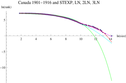
(a)

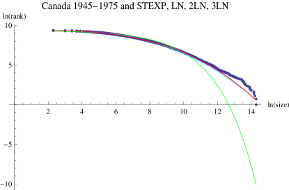
(b)

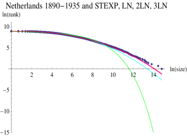
(c)

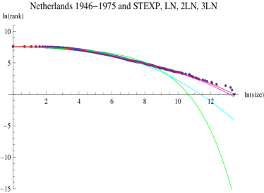
(d)

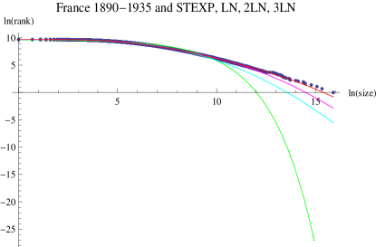
(e)

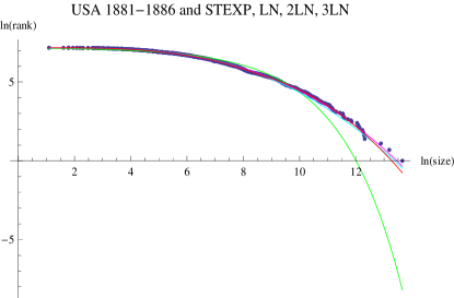
(f)

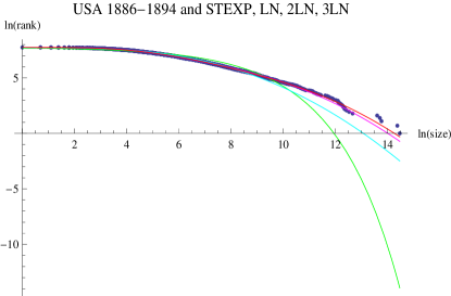
(g)

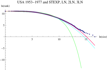
(h)

Figure 1: Log-rank plots for the whole samples of log-sizes, using the STEXP (green), LN (cyan), 2LN (magenta) and 3LN (red) distributions and the empirical data (blue). (In color online).

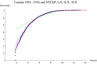
(a)

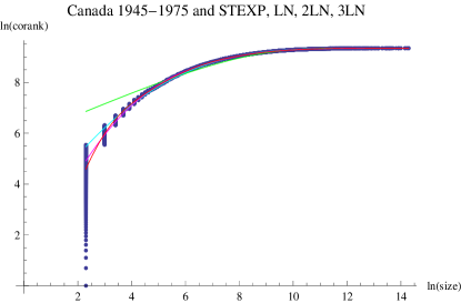
(b)

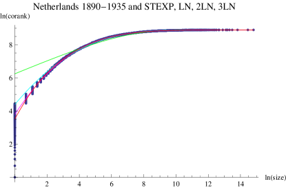
(c)

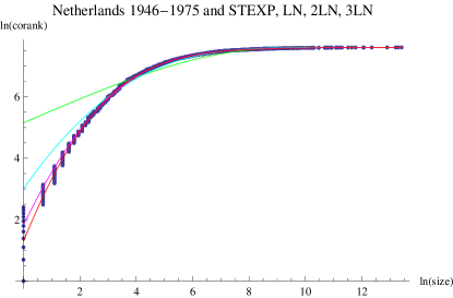
(d)

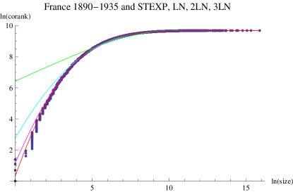
(e)

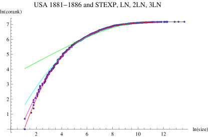
(f)

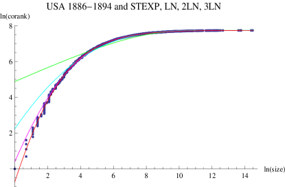
(g)

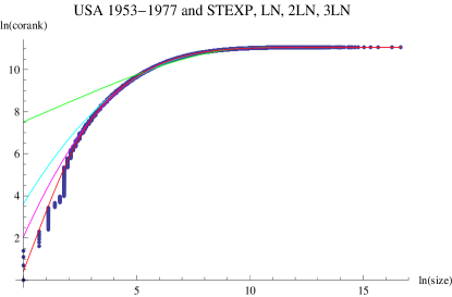
(h)

Figure 2: Log-corank plots for the whole samples of log-sizes, using the STEXP (green), LN (cyan), 2LN (magenta) and 3LN (red) distributions and the empirical data (blue). (In color online).

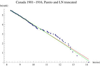
(a)

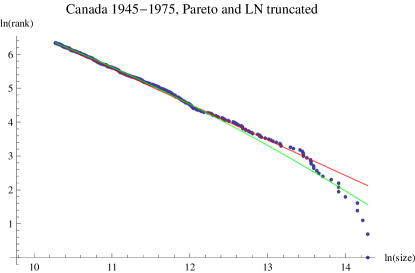
(b)

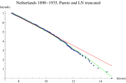
(c)

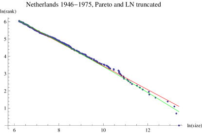
(d)

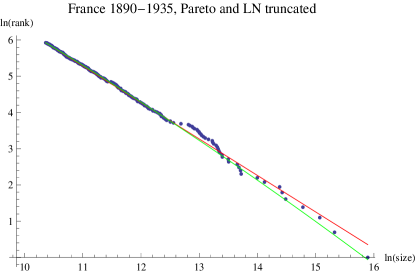
(e)

(f)

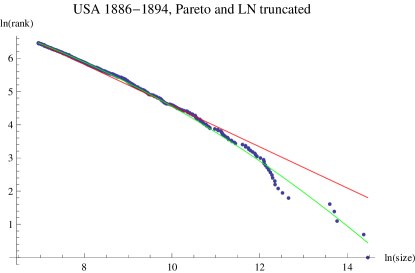
(g)

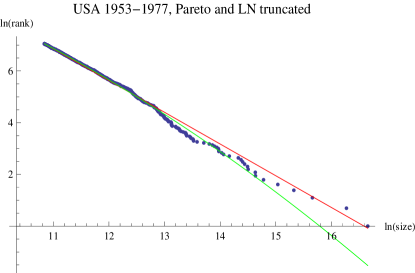
(h)

Figure 3: Log-rank plots for the upper tails, using the power law or Pareto distribution (red), the truncated lognormal LNt (green) and the empirical data (blue). (In color online).

We first consider a graphical approach to assessing goodness-of-fit with log-rank/corank plots. We have plotted these quantities for all the models we consider. The deviations at the upper (resp. lower) tails are amplified since we use logarithms (see, e.g., [32]). As is well known, the plot of the upper tails should be linear if the distribution in the tails is Pareto. We present these plots in Figures 1, 2 and 3, i.e., the plots of log-ranks, log-coranks for the whole samples and log-ranks for the upper tail samples, respectively.

In Figures 1 and 2, we observe that the fit of the STEXP is rather poor, meanwhile those of the 2LN and 3LN are really good (small discrepancies), and the LN performs a little worse than the second ones (larger discrepancies). We also observe a great deal of curvature in the data. In Figure 3, the discrepancies are also small and the data are approximately linear, making very hard to assess whether the Pareto or the truncated lognormal provides the best fit. Figure 3 illustrates the difficulty of distinguishing Pareto or power laws for the upper tails from other alternatives [52, 5, 6, 7, 58].

	STEXP
	KS	CM	AD
Canada 1901-1916	0 (0..088)	0 (2.987)	0 (21.965)
Canada 1945-1975	0 (0.089)	0 (23.456)	0 (167.264)
Netherlands 1890-1935	0 (0.090)	0 (19.660)	0 (134.767)
Netherlands 1946-1975	0 (0.129)	0 (11.597)	0 (74.266)
France 1890-1935	0 (0.103)	0 (51.602)	0 (358.700)
USA 1881-1886	0 (0.082)	0 (3.047)	0 (20.656)
USA 1886-1894	0 (0.110)	0 (10.157)	0 (65.858)
USA 1953-1977	0 (0.084)	0 (109.540)	0 (824.416)
	LN			2LN			3LN
	KS	CM	AD	KS	CM	AD	KS	CM	AD
Canada 1901-1916	0.513 (0.023)	0.526 (0.113)	0.396 (0.931)	0.582 (0.022)	0.526 (0.113)	0.492 (0.785)	0.893 (0.016)	0.990 (0.025)	0.995 (0.181)
Canada 1945-1975	0 (0.029)	0 (2.172)	0 (13.640)	0.019 (0.015)	0.192 (0.247)	0.031 (2.885)	0.028 (0.014)	0.464 (0.128)	0.059 (2.359)
Netherlands 1890-1935	0.001 (0.024)	0.004 (0.923)	0.001 (6.333)	0.251 (0.012)	0.572 (0.103)	0.386 (0.947)	0.579 (0.009)	0.664 (0.085)	0.475 (0.809)
Netherlands 1946-1975	0 (0.056)	0 (1.675)	0 (10.548)	0.030 (0.033)	0.393 (0.149)	0.462 (0.827)	0.402 (0.020)	0.899 (0.046)	0.932 (0.308)
France 1890-1935	0 (0.035)	0 (4.560)	0 (27.218)	0.082 (0.011)	0.359 (0.161)	0.258 (1.225)	0.302 (0.008)	0.814 (0.060)	0.861 (0.388)
USA 1881-1886	0.292 (0.027)	0.418 (0.141)	0.349 (1.017)	0.479 (0.023)	0.636 (0.090)	0.752 (0.494)	0.976 (0.013)	0.979 (0.029)	0.993 (0.190)
USA 1886-1894	0 (0.049)	0 (1.628)	0 (9.958)	0.792 (0.014)	0.760 (0.069)	0.759 (0.488)	0.920 (0.012)	0.993 (0.023)	0.996 (0.173)
USA 1953-1977	0 (0.024)	0 (5.439)	0 (35.790)	0.011 (0.008)	0.060 (0.431)	0.030 (2.923)	0.025 (0.007)	0.175 (0.261)	0.139 (1.680)
	Pareto			LNt
	KS	CM	AD	KS	CM	AD
Canada 1901-1916	0.965 (0.032)	0.960 (0.034)	0.420 (0.891)	0.925 (0.035)	0.948 (0.037)	0.398 (0.928)
Canada 1945-1975	0.865 (0.025)	0.698 (0.079)	0.582 (0.673)	0.906 (0.024)	0.905 (0.045)	0.769 (0.479)
Netherlands 1890-1935	0.285 (0.029)	0.197 (0.243)	0.084 (2.072)	0.423 (0.026)	0.570 (0.103)	0.166 (1.547)
Netherlands 1946-1975	0.821 (0.031)	0.692 (0.080)	0.104 (1.898)	0.593 (0.038)	0.535 (0.111)	0.083 (2.076)
France 1890-1935	0.997 (0.021)	0.986 (0.027)	0.958 (0.271)	0.866 (0.031)	0.965 (0.033)	0.946 (0.289)
USA 1881-1886	0.420 (0.063)	0.393 (0.149)	0.396 (0.931)	0.560 (0.056)	0.782 (0.065)	0.858 (0.390)
USA 1886-1894	0.163 (0.044)	0.118 (0.321)	0.042 (2.629)	0.924 (0.022)	0.915 (0.043)	0.256 (1.230)
USA 1953-1977	0.404 (0.026)	0.244 (0.213)	0.206 (1.387)	0.872 (0.018)	0.962 (0.034)	0.862 (0.387)

Table 4: Outcomes of the Kolmogorov–Smirnov (KS), Cramér–von Mises (CM) and Anderson–Darling (AD) tests, in the format $p$-value (test statistic). Non-rejections at the 5% level are marked in bold. Upper panels for the whole samples, lower panel for the truncated samples.

We also consider a more formal approach to goodness-of-fit with standard statistical tests. Table 4 presents the $p$-values (and test statistics in parentheses) for the Kolmogorov–Smirnov (KS), Cramér–von Mises (CM) and Anderson–Darling (AD) tests. The AD test is very well suited to studying the fit in the tails [17]. The $p$-values for all goodness-of-fit tests that we consider in Table 4 indicate that the STEXP distribution is soundly rejected as a plausible fit to the data for all the countries and times we consider. The $p$-values in Table 4 also show that the 2LN and 3LN distributions are very appropriate when considering the full range of the lost person days measure, and both the Pareto and LNt describe well the upper tail of the distributions. However, we should note that the power of these tests increases with the number of observations [54], so it might the case that the non-rejection of the different models is favored for the truncated samples.

	STEXP
	log-likelihood	AIC	BIC	HQC
Canada 1901-1916	-10883.8	21771.5	21781.8	21775.4
Canada 1945-1975	-102217	204439	204453	204444
Netherlands 1890-1935	-55040.9	110086	110100	110091
Netherlands 1946-1975	-14111.7	28227.3	28238.5	28231.4
France 1890-1935	-134924	269851	269867	269856
USA 1881-1886	-11660.3	23324.5	23334.8	23328.4
USA 1886-1894	-18821.6	37647.2	37658.7	37651.4
USA 1953-1977	-548415	1096833	1096852	1096839
	LN				2LN				3LN
	log-likelihood	AIC	BIC	HQC	log-likelihood	AIC	BIC	HQC	log-likelihood	AIC	BIC	HQC
Canada 1901-1916	-10725.4	21454.9	21465.1	21458.7	-10718.9	21447.77	21473.38	21457.4	-10709.6	21435.24	21476.21	21450.65
Canada 1945-1975	-100935	201874	201889	201879	-100847.8	201705.68	201742.42	201718.03	-100803	201622.76	201681.54	201642.52
Netherlands 1890-1935	-54104.6	108213	108227	108218	-54053.05	108116.1	108150.59	108127.96	-54047	108110.04	108165.23	108129.02
Netherlands 1946-1975	-13717.3	27438.6	27449.8	27442.7	-13647.72	27305.43	27333.45	27315.72	-13643.3	27302.65	27347.49	27319.11
France 1890-1935	-132433	264871	264886	264876	-132220.89	264451.78	264490.26	264464.5	-132199	264413.7	264475.27	264434.05
USA 1881-1886	-11529.7	23063.4	23073.7	23067.3	-11523.89	23057.78	23083.63	23067.48	-11519.6	23055.21	23096.57	23070.73
USA 1886-1894	-18448.4	36900.8	36912.3	36905	-18388.15	36786.31	36815.03	36796.78	-18383	36781.99	36827.95	36798.74
USA 1953-1977	-540534	1081072	1081091	1081078	-540116.21	1080242	1080288	1080256	-540024	1080064	1080136	1080086
	Pareto				LNt
	log-likelihood	AIC	BIC	HQC	log-likelihood	AIC	BIC	HQC
Canada 1901-1916	-2604.81	5211.61	5215.12	5213.02	-2608.22	5220.43	5227.45	5223.26
Canada 1945-1975	-6891.99	13785.98	13790.32	13787.68	-6891.58	13787.2	13795.8	13790.5
Netherlands 1890-1935	-11484.5	22970.98	22976.02	22972.88	-11488.9	22981.9	22991.9	22985.7
Netherlands 1946-1975	-3826.84	7655.68	7659.73	7657.28	-3833.46	7670.92	7679.01	7674.12
France 1890-1935	-4618.58	9239.15	9243.08	9240.71	-4619	9242	9249.85	9245.12
USA 1881-1886	-2205.59	4413.18	4416.47	4414.51	-2203.08	4410.17	4416.73	4412.83
USA 1886-1894	-6419.3	12840.61	12845.07	12842.34	-6419.67	12843.3	12852.3	12846.8
USA 1953-1977	-14405.3	28812.59	28817.64	28814.49	-14405.5	28815	28825.1	28818.8

Table 5: Maximum log-likelihoods, and outcomes of the AIC, BIC and HQC information criteria. The minimum values of these criteria for each sample are marked in bold. Upper panels for the whole samples, lower panel for the truncated samples.

In order to choose among the hypothesized models, we have computed the Akaike Information Criterion (AIC), the Bayesian or Schwarz Information Criterion (BIC) and the Hannan–Quinn Information Criterion (HQC), see Table 5. We note that the STEXP distribution is never chosen for any sample. The lognormal distribution is chosen by the BIC for the sample of Canada 1901-1916 and by both BIC and HQC for the sample of USA 1881-1886, so in these cases a single lognormal could provide a good description to the data. But in general, the information criteria differ in terms of the best distribution as they provide some conflicting evidence. The AIC tends to favor the 3LN, i.e., the mixture of 3 lognormal distributions. The BIC and HQC, often select the 3LN, but also favor the lognormal and 2LN, i.e., the mixture of 2 lognormal distributions. However, in the case of conflicting cases [10, 11] recommend relying on the AIC, based on information-theoretic arguments.

For the upper tail samples, it is feasible to compare the Pareto with the LNt in another way: since they are non-nested models, it is possible to perform Vuong tests [68] to assess whether the models are statistically equivalent (null hypothesis) or one of the models is favored (alternative hypothesis). Positive test statistics are supportive of the power law distribution, but negative values would suggest the truncated lognormal distribution would be more appropriate. We see in Table 6 that we cannot distinguish between the Pareto and the LNt distributions as are statistically equivalent models most of the cases. The two exceptions are Canada 1901-1916 and Netherlands 1946-1935, where the tests support a power law distribution.

	Vuong Pareto vs LNt
Canada 1901-1916	0.034 (2.125)
Canada 1945-1975	0.849 (-0.191)
Netherlands 1890-1935	0.244 (1.166)
Netherlands 1946-1975	0.005 (2.784)
France 1890-1935	0.652 (0.451)
USA 1881-1886	0.265 (-1.114)
USA 1886-1894	0.931 (0.087)
USA 1953-1977	0.945 (0.069)

Table 6: Outcomes of Vuong tests of Pareto vs LNt distributions for the upper tail. The format is $p$-value (test statistic). Non-rejections at the 5% level are marked in bold.

From a statistical perspective, the lognormal distribution is very often inferior to a mixture of lognormal distributions. This is not surprising as the summary statistics indicate that there is a great deal of skew and kurtosis in the lost person days measure of strike size and a mixture of lognormal distributions is better able to capture this feature of the data. The AIC, the preferred information criterion, suggests that this is true across the countries and time periods we consider. This consistency of our finding suggests that there could a common process shaping strikes, e.g., legislative, economic or social factors, across time and the countries we consider. In the upper tail of the data, it is much more difficult to distinguish the power law from the truncated lognormal distribution, but this should not be overly surprising given the results in recent empirical work [52, 5, 6, 7, 58].

5 Conclusions

We have studied the distribution of strike size using data from the late-19th and 20th centuries in some European countries, Canada and the US. There are remarkable regularities for this variable that reflect in its parametric distribution. First, we find that strike size, for the different samples we consider, can be faithfully described by a mixture of two or three lognormals (2LN, 3LN in the notation above), as it happens as well for some samples of city sizes [43, 12, 61, 53]. Second, finding a common distribution across countries and time periods also suggests that the distribution of strikes could be shaped by common forces, which could be economic, legislative or social in nature. Third, when restricting the data to the upper tail, the identification of the appropriate model becomes more problematic. We have studied, because of their importance, the Pareto and (upper-tail) truncated lognormal. The results of Vuong test show that they are statistically equivalent in most of the cases we consider, although there are some exceptions that favor the Pareto. Thus the upper tail can be described by a power law, although it should not considered as a unique model for this purpose.

Author contributions

Michele Campolieti: Conceptualization, data curation, formal analysis, investigation, methodology, software, supervision, validation, visualization, writing-original draft, writing-review & editing. Arturo Ramos: Conceptualization, data curation, formal analysis, funding acquisition, investigation, methodology, resources, software, validation, visualization, writing-original draft, writing-review & editing.

Competing interests statement

The authors declare to have no competing interests concerning the research carried out in this article.

Data appendix

The data for the Dutch strikes were obtained from the following webpage:

https://collab.iisg.nl/web/labourconflicts/datafiles

The Dutch data, known as SIN (Strikes in the Netherlands or, equivalently, Stakingen in Nederland) were collected by Sjaak van der Velder and are described in [66].

French strike data were collected by [60] and are available via the ICPSR at the University of Michigan.

https://www.icpsr.umich.edu/index.html

The Canadian data for 1901-1916 were obtained via the Labour Conflicts Dataverse

https://datasets.socialhistory.org/dataset.xhtml?persistentId=hdl:10622/J5TJNF

They were compiled by [57] based on the records kept by the Department of Labour, Canada.

The Canada data for 1946-1975 were obtained from the Labour Program, Government of Canada by request

https://www.canada.ca/en/employment-social-development/services/labour-contact.html

U.S. data for 1881-1886 and 1886-1894 were collected from the 3rd and 10th Annual Reports of the U.S. Commissioner of Labour [64, 65].

U.S. data for 1953-1977 are available via the ICPSR at the University of Michigan.

References

- Akaike, [1974] Akaike, H. (1974). A new look at the statistical model identification. IEEE Transactions on Automatic Control, 19(6):716–723.
- Amemiya, [1980] Amemiya, T. (1980). Selection of regressors. International Economic Review, 21:331–354.
- Axtell, [2001] Axtell, R. (2001). Zipf distribution of U.S. firm sizes. Science, 293(5536):1818–1820.
- Bak and Chen, [1991] Bak, P. and Chen, K. (1991). Self-organized criticality. Scientific American, 264(1):46–53.
- Bee et al., [2011] Bee, M., Riccaboni, M., and Schiavo, S. (2011). Pareto versus lognormal: a maximum entropy test. Physical Review E, 84:026104.
- Bee et al., [2013] Bee, M., Riccaboni, M., and Schiavo, S. (2013). The size distribution of US cities: not Pareto, even in the tail. Economics Letters, 120:232–237.
- Bee et al., [2019] Bee, M., Riccaboni, M., and Schiavo, S. (2019). Distribution of city size: Gibrat, Pareto, Zipf. In D’Acci, L., editor, The Mathematics of Urban Morphology. Springer Nature Switzerland.
- Biggs, [2005] Biggs, M. (2005). Strikes as forest fires: Chicago and Paris in the late Nineteenth Century. American Journal of Sociology, 110(6):1684–1714.
- Biggs, [2018] Biggs, M. (2018). Size matters: Quantifying protest by counting participants. Sociological Methods and Research, 47(3):351–383.
- Burnham and Anderson, [2002] Burnham, K. P. and Anderson, D. R. (2002). Model selection and multimodel inference: A practical information-theoretic approach. New York: Springer-Verlag.
- Burnham and Anderson, [2004] Burnham, K. P. and Anderson, D. R. (2004). Multimodel inference: Understanding AIC and BIC in model selection. Sociological Methods and Research, 33:261–304.
- Bǎncescu et al., [2019] Bǎncescu, I., Chivu, L., Preda, V., Puente-Ajovín, M., and Ramos, A. (2019). Comparisons of log-normal mixture and pareto tails, GB2 or log-normal body of Romania’s all cities size distribution. Physica A: Statistical Mechanics and its Applications, 526:121017.
- Campolieti, [2018] Campolieti, M. (2018). Heavy-tailed distributions and the distribution of wealth: Evidence from rich lists in Canada, 1999-2017. Physica A: Statistical Mechanics and its Applications, 503:263–272.
- Campolieti, [2019] Campolieti, M. (2019). Power law distributions and the size distribution of strikes. Sociological Methods and Research, 48:561–587.
- Campolieti, [2020] Campolieti, M. (2020). The distribution of union size: Canada, 1913-2014. Physica A: Statistical Mechanics and its Applications, 558:125007.
- Cederman, [2003] Cederman, L.-K. (2003). Modelling the size of wars: From billiard balls to sandpiles. American Political Science Review, 97(1):135–150.
- Cirillo, [2013] Cirillo, P. (2013). Are your data really Pareto distributed? Physica A: Statistical Mechanics and its Applications, 392:5947–5962.
- Clauset et al., [2009] Clauset, A., Shalizi, C. R., and Newman, E. J. (2009). Power-law distributions in empirical data. SIAM Review, 51(4):661–703.
- Clauset et al., [2007] Clauset, A., Young, M., and Skrede Gleditsch, K. (2007). On the frequency of severe terrorist attacks. Journal of Conflict Resolution, 51(1):58–87.
- Dolfin et al., [2017] Dolfin, M., Leonida, L., and Outada, N. (2017). Modeling human behavior in economics and social science. Physics of Life Reviews, 22-23:1–21.
- Dupire, [1993] Dupire, B. (1993). Pricing and hedging with smiles. In Proceedings of AFFI Conference, La Baule, June.
- Efron and Hinkley, [1978] Efron, B. and Hinkley, D. V. (1978). Assessing the accuracy of the maximum likelihood estimator: Observed versus expected Fisher information. Biometrika, 65(3):457–482.
- Fattorini and Lemmi, [2006] Fattorini, L. and Lemmi, A. (2006). The stochastic interpretation of the Dagum personal income distribution: a tale. Statistica, LXVI(3):325–329.
- Freeman, [1998] Freeman, R. B. (1998). Spurts in union growth: Defining moments and social processes. In Bordo, M. D. and Goldin, C. White, E. N., editors, The Defining Moment: The Great Depression and the American Economy in the Twentieth Century, pages 265–296. University of Chicago Press, Chicago.
- Friedman, [2015] Friedman, J. A. (2015). Using power laws to estimate conflict size. Journal of Conflict Resolution, 59(7):1216–1241.
- Frisch and Sornette, [1997] Frisch, U. and Sornette, D. (1997). Extreme deviations and applications. Journal de Physique I France, 7:1155–1171.
- Furioli et al., [2017] Furioli, G., Pulvirenti, A., Terraneo, E., and Toscani, G. (2017). Fokker–Planck equations in the modeling of socio-economic phenomena. Mathematical Models and Methods in Applied Sciences, 27(1):115–158.
- Gabaix, [1999] Gabaix, X. (1999). Zipf’s law for cities: An explanation. Quarterly Journal of Economics, 114:739–767.
- Gabaix, [2009] Gabaix, X. (2009). Power laws in Economics and finance. Annu. Rev. Econ., 2009:255–293.
- Gardiner, [2004] Gardiner, C. W. (2004). Handbook of stochastic methods for Physics, Chemistry and the Natural Sciences (third edition). Springer.
- González-Val, [2015] González-Val, R. (2015). War size distribution: Empirical regularities behind conflicts. Defence and Peace Economics, 27:838–853.
- González-Val et al., [2013] González-Val, R., Ramos, A., and Sanz-Gracia, F. (2013). The accuracy of graphs to describe size distributions. Applied Economics Letters, 20(17):1580–1585.
- Gualandi and Toscani, [2018] Gualandi, S. and Toscani, G. (2018). Call center service times are lognormal: a Fokker–Planck description. Mathematical Models and Methods in Applied Sciences, 28(8):1513–1527.
- [34] Gualandi, S. and Toscani, G. (2019a). Human behavior and lognormal distribution. A kinetic description. Mathematical Models and Methods in Applied Sciences, 29(4):717–753.
- [35] Gualandi, S. and Toscani, G. (2019b). Size distribution of cities: A kinetic explanation. Physica A: Statistical Mechanics and its Applications, 524:221–234.
- Hamilton, [1994] Hamilton, J. D. (1994). Time series analysis. Princeton University Press, Princeton.
- Hannan and Quinn, [1979] Hannan, E. J. and Quinn, B. G. (1979). The Determination of the order of an autoregression. Journal of the Royal Statistical Society, Series B, 41:190–195.
- Herbert and Bonini, [1958] Herbert, S. and Bonini, C. P. (1958). The size distribution of business firms. American Economic Review, 48(4):607–617.
- Itô and McKean Jr., [1996] Itô, K. and McKean Jr., H. P. (1996). Diffusion processes and their sample paths (reprint of the 1974 edition). Springer.
- Jiang et al., [2013] Jiang, Z.-Q., Xie, W.-J., Li, M.-X., Podobnik, B., Zhou, W.-X., and Stanley, H. E. (2013). Calling patterns in human communication dynamics. Proceedings of the National Academy of Sciences of the United States of America, 110(5):1600–1605.
- Kalecki, [1945] Kalecki, M. (1945). On the Gibrat distribution. Econometrica, 13(2):161–170.
- Krugman, [1996] Krugman, P. (1996). The self-organizing Economy. Blackwell Publishers, Cambridge.
- Kwong and Nadarajah, [2019] Kwong, H. S. and Nadarajah, S. (2019). A note on “Pareto tails and lognormal body of US cities size distribution”. Physica A: Statistical Mechanics and its Applications, 513:55–62.
- Kyprianou, [2006] Kyprianou, A. E. (2006). Introductory lectures on fluctuations of Lévy processes with applications. Springer-Verlag.
- Laherrère and Sornette, [1998] Laherrère, J. and Sornette, D. (1998). Stretched exponential distributions in nature and economy:“fat tails” with characteristic scales. European Physical Journal B-Condensed Matter and Complex Systems, 2:525–539.
- McCullough and Vinod, [2003] McCullough, B. D. and Vinod, H. D. (2003). Verifying the solution from a nonlinear solver: A case study. American Economic Review, 93(3):873–892.
- McLachlan and Peel, [2003] McLachlan, G. and Peel, D. (2003). Finite mixture models. Wiley-Interscience.
- Mitzenmacher, [2004] Mitzenmacher, M. (2004). A brief history of generative models for power law and log normal distributions. Internet Mathematics, 1(2):226–251.
- Moghaddam et al., [2020] Moghaddam, M. D., Mills, J., and Serota, R. A. (2020). From a stochastic model of economic exchage to measures of inequality. Physica A: Statistical Mechanics and its Applications, 559:125047.
- Ord, [1974] Ord, J. K. (1974). Statistical Distributions in Scientific Work. Volume 2–Model Building and Model Selection, chapter Statistical models for personal income distributions. D. Reidel Publishing Company.
- Pencavel, [2014] Pencavel, J. (2014). The changing size distributions of U.S. trade unions and its description by Pareto’s distribution. Industrial and Labor Relations Review, 67(1):138–170.
- Perline, [2005] Perline, R. (2005). Strong, weak and false inverse power laws. Statistical Science, 20(1):68–88.
- Puente-Ajovín et al., [2020] Puente-Ajovín, M., Ramos, A., and Sanz-Gracia, F. (2020). Is there a universal parametric city size distribution? empirical evidence for 70 countries. The Annals of Regional Science.
- Razali and Wah, [2011] Razali, N. M. and Wah, Y. B. (2011). Power comparisons of Shapiro-Wilk, Kolmogorov-Smirnov, Lilliefors and Anderson-Darling tests. Journal of Statistical Modeling and Analytics, 2:21–33.
- Richardson, [1948] Richardson, L. F. (1948). Variation of the frequency of fatal quarrels with magnitude. American Statistical Association, 43(244):523–546.
- Roberts and Turcotte, [1998] Roberts, D. C. and Turcotte, D. L. (1998). Fractality and self-organized criticality of wars. Fractals, 6(4):351–357.
- Rosero, S., [2017] Rosero, S. (2017). Canada, 1901-1916. IISH Dataverse, V1. http://hdl.handle.net/10622/J5TJNF.
- Schluter and Trede, [2018] Schluter, C. and Trede, M. (2018). Size distributions reconsidered. Econometric Reviews.
- Schwarz, [1978] Schwarz, G. E. (1978). Estimating the dimension of a model. Annals of Statistics, 6(2):461–464.
- Shorter and Tilly, [1974] Shorter, E. and Tilly, C. (1974). Strikes in France, 1830–1868. Cambridge University Press, New York.
- Su, [2020] Su, H.-L. (2020). On the city size distribution: A finite mixture interpretation. Journal of Urban Economics, 116:103216.
- Tomaschitz, [2020] Tomaschitz, R. (2020). Multiply broken power law densities as survival functions: An alternative to Pareto and lognormal fits. Physica A: Statistical Mechanics and its Applications, 541:123188.
- Uhlenbeck and Ornstein, [1930] Uhlenbeck, G. E. and Ornstein, L. S. (1930). On the theory of the Brownian motion. Physical Review, 36:823–841.
- U.S. Commissioner of Labor, [1888] U.S. Commissioner of Labor (1888). Third annual report. 1888. Washington: Government Printing Office.
- U.S. Commissioner of Labor, [1896] U.S. Commissioner of Labor (1896). Tenth annual report. 1896. Washington: Government Printing Office.
- van der Velder, [2003] van der Velder, S. (2003). Strikes in global labor history: The Dutch case. Review (Fernand Braudel Center), 26(4):381–405.
- Vasicek, [1977] Vasicek, O. (1977). An equilibrium characterization of the term structure. Journal of Financial Economics, 5:177–188.
- Vuong, [1989] Vuong, Q. H. (1989). Likelihood ratio tests for model selection and non-nested hypotheses. Econometrica, 57(2):307–333.