Noisy-Correspondence Learning for Text-to-Image Person Re-identification

Abstract

Text-to-image person re-identification (TIReID) is a compelling topic in the cross-modal community, which aims to retrieve the target person based on a textual query. Although numerous TIReID methods have been proposed and achieved promising performance, they implicitly assume the training image-text pairs are correctly aligned, which is not always the case in real-world scenarios. In practice, the image-text pairs inevitably exist under-correlated or even false-correlated, a.k.a noisy correspondence (NC), due to the low quality of the images and annotation errors. To address this problem, we propose a novel Robust Dual Embedding method (RDE) that can learn robust visual-semantic associations even with NC. Specifically, RDE consists of two main components: 1) A Confident Consensus Division (CCD) module that leverages the dual-grained decisions of dual embedding modules to obtain a consensus set of clean training data, which enables the model to learn correct and reliable visual-semantic associations. 2) A Triplet-Alignment Loss (TAL) relaxes the conventional triplet-ranking loss with hardest negatives, which tends to rapidly overfit NC, to a log-exponential upper bound over all negatives, thus preventing the model from overemphasizing false image-text pairs. We conduct extensive experiments on three public benchmarks, namely CUHK-PEDES, ICFG-PEDES, and RSTPReID, to evaluate the performance and robustness of our RDE. Our method achieves state-of-the-art results both with and without synthetic noisy correspondences on all three datasets.

Introduction

Text-to-image person re-identification (TIReID) (Li et al. 2017; Shu et al. 2022; Jiang and Ye 2023) aims to understand the natural language descriptions to retrieve the matched person image from a large gallery set. This task has received increasing attention from both academic and industrial communities recently, e.g., finding/tracking suspect/lost persons in a surveillance system (Wang et al. 2015; Eom and Ham 2019). However, TIReID remains a challenging task due to the inherent heterogeneity gap across different modalities and appearance attribute redundancy.

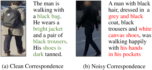
Figure 1: The illustration of noisy correspondence. The figure shows an example of the NC problem, which occurs when the image-text pairs are wrongly aligned, i.e., false positive pairs (FPPs). Since the model does not know which pairs are noisy in practice, they will unavoidably degrade the performance by incorrect supervision information. As seen in the figure, (a) the clean image-text pair is semantically matched, while (b) the noisy pair is not, which would cause the cross-modal model to learn erroneous visual-textual associations. Note that both examples in (a) and (b) are from and actually exist in the RSTPReid dataset (Zhu et al. 2021).

To tackle these challenges, most of the existing methods explore global- and local-matching alignment to learn accurate similarity measurements for person re-identification. To be specific, some global-matching methods (Zhang and Lu 2018; Wu et al. 2021; Shu et al. 2022) leverage vision/language backbones to extract modality-specific features and employ contrastive learning to achieve global visual-semantic alignments. To capture fine-grained information, some local-matching methods (Niu et al. 2020; Jing et al. 2020; Wang et al. 2021; Shao et al. 2022) explicitly align local body regions to textually described entities/objectives to improve the discriminability of pedestrian features. Recently, some works (Han et al. 2021; Yan et al. 2022a; Jiang and Ye 2023) propose to exploit visual/semantic knowledge learned by the pre-trained models, such as BERT (Devlin et al. 2018), ViT (Dosovitskiy et al. 2020), and CLIP (Radford et al. 2021), and achieve explicit global alignments or discover more fine-grained local correspondence, thus boosting the re-identification performance. Although these methods achieve remarkable progress, they implicitly assume that all training image-text pairs are aligned correctly.

In reality, this assumption is hard or even impossible to hold due to the person’s pose, camera angle, illumination, and other inevitable factors in images, which may result in some inaccurate/mismatched textual descriptions of images (see Figure 6), e.g., the RSTPReid dataset (Zhu et al. 2021). Moreover, we observe that excessive such imperfect/mismatched image-text pairs would cause an overfitting problem and degrade the performance of existing TIReID methods shown in Figure 4. Based on the observation, in this paper, we reveal and study a new problem in TIReID, i.e., noisy correspondence (NC). Different from noisy labels, NC refers to the false correspondences of image-text pairs in TIReID, i.e., False Positive Pairs (FPPs): some negative image-text pairs are used as positive ones for cross-modal learning. Inevitably, FPPs will misguide models to overfit noisy supervision and collapse to suboptimal solutions due to the memorization effect (Arpit et al. 2017) of Deep Neural Networks (DNNs).

To address the NC problem, we propose a Robust Dual Embedding method (RDE) for TIReID in this paper, which benefits from an effective Confident Consensus Division mechanism (CCD) and a novel Triplet-Alignment Loss (TAL). Specifically, CCD fuses the dual-grained decisions to consensually divide the training data into clean and noisy sets, thus providing more reliable correspondences for robust learning. To diversify the model grain, the basic global embeddings (BGE) and token selection embeddings (TSE) are presented for coarse-grained and fine-grained cross-modal interactions respectively, thus capturing visual-semantic associations comprehensively. Different from the widely-used Triplet-Ranking loss with hardest negatives, which tends to overfit NC, our TAL relaxes the similarity learning from the hardest negative samples to all negative ones. This prevents the optimization from being dominated by the hardest negatives, and makes training more stable and less prone to misleading risks. Therefore, our RDE can achieve robustness against NC thanks to the proposed reliable supervision and robust loss. The contributions and innovations of this paper are summarized as follows:

• We reveal and study a new and ubiquitous problem in TIReID, termed noisy correspondence (NC). Different from class-level noisy labels, NC refers to erroneous correspondences in the person-description pairs that can mislead the model to learn incorrect visual-semantic associations. To the best of our knowledge, this paper could be the first work to explore this problem in TIReID.

• We propose a robust method, termed RDE, to mitigate the adverse impact of NC through the proposed Confident Consensus Division (CCD) and novel Triplet-Alignment Loss (TAL). By using CCD and TAL, our RDE could obtain convincing consensus pairs and reduce the misleading risks in training, thus embracing robustness against NC.

• Extensive experiments on three public image-text person benchmarks demonstrate the robustness and superiority of our method. Our method achieves the best performance both with and without synthetic noisy correspondence on all three datasets.

Related Work

Text-to-Image Person Re-identification

Text-to-image person re-identification (TIReID) is a novel and challenging task that aims to match a person image with a given natural language description (Li et al. 2017; Zhang and Lu 2018). Existing TIReID methods could be roughly classified into two groups according to their alignment levels, i.e., global-matching methods (Shu et al. 2022; Zheng et al. 2020; Zhu et al. 2021) and local-matching methods (Gao et al. 2021; Wang et al. 2021; Shao et al. 2022). The former try to learn cross-modal embeddings in a common latent space by employing textual and visual backbones with a matching loss (e.g., CMPM/C loss (Zhang and Lu 2018) and Triplet-Ranking loss (Faghri et al. 2017)) for TIReID. However, these methods mainly focus on global features while ignoring the fine-grained interactions between local features, which limits their performance improvement. To achieve fine-grained interactions, some of the latter methods explore explicit local alignments between body regions and textual entities for more refined alignments. However, these methods require more computational resources due to the complex local-level associations. Recently, inspired and benefited from vision-language pre-training models (Radford et al. 2021), some methods (Han et al. 2021; Yan et al. 2022a; Jiang and Ye 2023) expect to use the learned rich alignment knowledge of pre-trained models for local- or global-alignments. Although these methods achieve promising performance, almost all of them implicitly assume that all input training pairs are correctly aligned, which is hard to meet in practice due to the ubiquitous noise. In this paper, we address the inevitable and challenging noisy correspondence problem in TIReID.

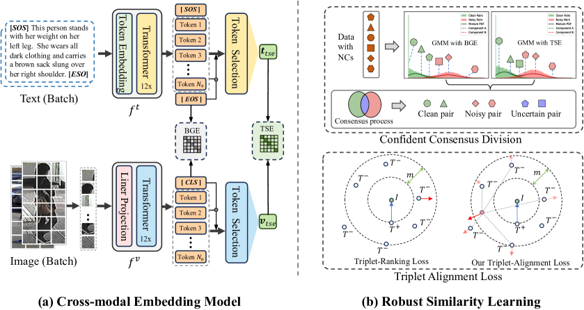
Figure 2: The overview of our RDE. (a) is the illustration of the cross-modal embedding model used in RDE, which consists of basical global embedding (BGE) and token selection embedding (TSE) modules with different granularity. By integrating them, RDE can capture coarse-grained cross-modal interactions while selecting informative local token features to encode more fine-grained representations for a more accurate similarity. (b) shows the core of RDE to achieve robust similarity learning, which consists of Confident Consensus Division (CCD) and Triplet-Alignment Loss (TAL). CCD performs consensus division to obtain confident clean training data, thus avoiding misleading from noisy pairs. Unlike traditional Triplet-Ranking Loss (TRL) (Faghri et al. 2017), TAL exploits an upper bound to consider all negative pairs, thus embracing more stable learning.

Learning with Noisy Correspondence

As a special learning paradigm with noisy labels (Li, Socher, and Hoi 2020; Lu, Bo, and He 2022; Feng et al. 2023) in multi-modal community, the studies for noisy correspondence (NC) have recently attracted more and more attention in various tasks, e.g., video-text retrieval (Zhang et al. 2023), visible-infrared person re-identification (Yang et al. 2022), and image-text matching (Huang et al. 2021; Qin et al. 2022), which means that the negative pairs are wrongly treated as positive ones, i.e., false positive pairs (FPPs). To handle this problem, numerous methods are proposed to learn with NC, which can be broadly categorized into sample selection (Huang et al. 2021; Zhang et al. 2023; Han et al. 2023) and robust loss functions (Yang et al. 2022; Qin et al. 2022; Hu et al. 2023). The former commonly leverage the memorization effect of DNNs (Arpit et al. 2017) to gradually distinguish the noisy data, thus paying more attention to clean data while less attention to noisy data. Differently, the latter methods aim to develop noise-tolerance loss functions to improve the robustness of model training against NC. Although the aforementioned methods achieve promising performance in various tasks, they are not specifically designed for TIReID and may be inefficient or ineffective in person re-identification. In this paper, we propose a well-designed method to tackle the NC problem in TIReID, which not only performs superiority in noisy scenarios but also achieves state-of-the-art performance in ordinary scenarios.

Methodology

Problem Statement

The purpose of TIReID is to retrieve a pedestrian image from the gallery set that matched the given textual description. For clarity, we represent the gallery set as $\mathcal{V}=\{I_{i},y^{p}_{i},y^{v}_{i}\}^{N_{v}}_{i=1}$ and the corresponding text set as $\mathcal{T}=\{T_{i},y^{v}_{i}\}^{N_{t}}_{i=1}$, where $N_{v}$ is the number of images, $N_{t}$ is the number of texts, $y^{p}_{i}\in\mathcal{Y}_{p}=\{1,\cdots,C\}$ is the class label (person identify), $C$ is the number of identifies, and $y^{v}_{i}\in\mathcal{Y}_{v}=\{1,\cdots,N_{v}\}$ is the image label. The image-text pair set used in TIPeID can be defined as $\mathcal{P}=\{(I_{i},T_{i}),y^{v}_{i},y^{p}_{i}\}^{N}_{i=1}$, where the cross-modal samples of each pair have the same image label $y_{i}^{v}$ and class label $y_{i}^{p}$. We define a binary correspondence label $l_{ij}\in\{0,1\}$ to indicate the matched degree of any image-text pair. If $l_{ij}=1$, the pair $(I_{i},T_{j})$ is matched (positive pair), otherwise it is not (negative pair). In practice, due to ubiquitous annotation noise, some unmatched pairs $(l_{ij}=0)$ are wrongly labeled as matched $(l_{ij}=1)$, resulting in noisy correspondences (NCs) and performance degradation. To handle NC for robust TIReID, we present an RDE that leverages the Confident Consensus Division (CCD) and Triplet-Alignment Loss (TAL) to mitigate the negative impact of label noise.

Cross-modal Embedding Model

In this section, we describe the cross-modal model used in our RDE. Following previous work (Jiang and Ye 2023), we utilize the visual encoder $f^{v}$ and textual encoder $f^{t}$ of the pre-trained model CLIP as modality-specific encoders to obtain token representations and implement cross-modal interactions through two embedding modules.

Token Representations

Give an input image $I_{i}\in\mathcal{V}$, we use the visual encoder $f^{v}$ of CLIP to tokenize the image into a discrete token representation sequence with a length of $N_{\circ}+1$, i.e., $\boldsymbol{V}_{i}=f^{v}(I_{i})=\{\boldsymbol{v}^{i}_{g},\boldsymbol{v}^{i}_{1},\boldsymbol{v}^{i}_{2},\cdots,\boldsymbol{v}^{i}_{N_{\circ}}\}\in\mathbb{R}^{(N_{\circ}+1)\times d}$, where $d$ is the dimensionality of the shared latent space. These features include an encoded feature $\boldsymbol{v}^{i}_{g}$ of the [CLS] token and patch-level local features $\{\boldsymbol{v}^{i}_{j}\}^{N_{\circ}}_{j=1}$ of $N_{\circ}$ fixed-sized non-overlapping patches of $I_{i}$, wherein $\boldsymbol{v}^{i}_{g}$ can represent the global representation. For an input text $T_{i}\in\mathcal{T}$, we apply the textual encoder $f^{t}$ of CLIP to obtain global and local representations. Specifically, following IRRA (Jiang and Ye 2023), we first tokenize the input text $T_{i}$ using lower-cased byte pair encoding (BPE) with a 49,152 vocab size into a token sequence. The token sequence is bracketed with [SOS] and [EOS] tokens to represent the beginning and end of the sequence. Then, we feed the token sequence into $f_{t}$ to obtain the features $\boldsymbol{T}_{i}=\{\boldsymbol{t}^{i}_{s},\boldsymbol{t}^{i}_{1},\cdots,\boldsymbol{t}^{i}_{N_{\diamond}},\boldsymbol{t}^{i}_{e}\}\in\mathbb{R}^{(N_{\diamond}+2)\times d}$, where $\boldsymbol{t}^{i}_{s}$ and $\boldsymbol{t}^{i}_{e}$ are the features of [SOS] and [EOS] tokens and $\{\boldsymbol{v}_{j}^{i}\}^{N_{\diamond}}_{j=1}$ are the word-level local features of $N_{\diamond}$ word tokens of text $T_{i}$. Generally, the $\boldsymbol{t}^{i}_{e}$ can be regarded as the sentence-level global feature of $T_{i}$.

Dual Embedding Modules.

To measure the similarity between any image-text pair $(I_{i},T_{j})$, we can directly use the global features of [CLS] and [EOS] tokens to compute the Basic Global Embedding (BGE) similarity by the cosine similarity, i.e., $S^{b}_{ij}={{\boldsymbol{v}^{i}_{g}}^{\top}\boldsymbol{t}^{j}_{e}}\big{/}{\|\boldsymbol{v}^{i}_{g}\|\|\boldsymbol{t}^{j}_{e}\|}$, where the global features represent the global embedding representations of two modalities. However, optimizing the BGE similarities alone may not capture the fine-grained interactions between two modalities, which will limit performance improvement. To address this issue, we exploit the local features of informative tokens to learn more discriminative embedding representations, thus mining the fine-grained correspondences. In CLIP, the global features of the tokens ([CLS] and [EOS]) are obtained by a weighted aggregation of all local token features. These weights reflect the correlation between the global token and each local token. Following previous methods (Yan et al. 2022a; Zhu et al. 2022), we could select the informative tokens based on these correlation weights to aggregate local features for a more representative global embedding.

In practice, these correlation weights can be obtained directly in the self-attention map of the last Transformer blocks of $f^{v}$ and $f^{t}$, which reflects the relevance among the input $1+N_{\circ}$ (or $2+N_{\diamond}$) tokens. Given the output self-attention map $\boldsymbol{A}^{v}_{i}\in\mathbb{R}^{(1+N_{\circ})\times(1+N_{\circ})}$ of image $I_{i}$, the correlation weights between global token and local tokens are $\{a^{v}_{i,j}\}^{N_{\circ}}_{j=1}=\boldsymbol{a}^{v}_{i}=\boldsymbol{A}^{v}_{i}[0,1:N_{\circ}+1]\in\mathbb{R}^{N_{\circ}}$. Similarly, for text $T_{i}$, the correlation weights are $\{a^{t}_{i,j}\}^{N_{\diamond}}_{j=1}=\boldsymbol{a}^{t}_{i}=\boldsymbol{A}^{t}_{i}[0,1:N_{\diamond}+1]\in\mathbb{R}^{N_{\diamond}}$, where $\boldsymbol{A}^{t}_{i}\in\mathbb{R}^{(2+N_{\diamond})\times(2+N_{\diamond})}$ is the output self-attention map for text $I_{i}$. Then, we select a proportion ($TopK$) of the corresponding token features with higher scores for embedding. Specifically, for $I_{i}$, the selected token sequences and correlation weights are reorganized as $\boldsymbol{V}^{s}_{i}=\{\boldsymbol{v}^{i}_{j}\}_{j\in\boldsymbol{K}^{v}_{i}}$ and $\hat{\boldsymbol{a}}^{v}_{i}=\{a^{v}_{i,j}\}_{j\in\boldsymbol{K}^{v}_{i}}$, where $\boldsymbol{K}^{v}_{i}\in\mathbb{R}^{\lfloor\mathcal{R}N_{\circ}\rfloor}$ is the set of indices for the selected local tokens of $I_{i}$ and $\mathcal{R}$ is the selection ratio. For text $T_{i}$, the selected token sequences and correlation weights are also reorganized as $\boldsymbol{T}^{s}_{i}=\{\boldsymbol{t}^{i}_{j}\}_{j\in\boldsymbol{K}^{t}_{i}}$ and $\hat{\boldsymbol{a}}^{t}_{i}=\{a^{t}_{i,j}\}_{j\in\boldsymbol{K}^{t}_{i}}$, where $\boldsymbol{K}^{t}_{i}\in\mathbb{R}^{\lfloor\mathcal{R}N_{\diamond}\rfloor}$ is the set of indices for the selected local tokens of $T_{i}$. For $I_{i}$ and $T_{i}$, we perform an embedding transformation on these selected token features to obtain subtle representations, instead of using complex fine-grained correspondence discovery used in CFine (Yan et al. 2022a). The transformation is performed by an embedding module like the residual block (He et al. 2016), as follows:

$$\boldsymbol{v}^{i}_{tse}= {MaxPool}({MLP(\hat{\boldsymbol{I}}^{s}_{i})}+FC(\hat{\boldsymbol{I}}^{s}_{i})),$$ (1)

$$\boldsymbol{t}^{i}_{tse}= {MaxPool}({MLP(\hat{\boldsymbol{T}}^{s}_{i})}+FC(\hat{\boldsymbol{T}}^{s}_{i})),$$

where $MaxPool(\cdot)$ is the max-pooling function, $MLP(\cdot)$ is a multi-layer perceptron (MLP) layer, $FC(\cdot)$ is a linear layer, $\hat{\boldsymbol{I}}^{s}_{i}=L2Norm({\boldsymbol{I}}^{s}_{i})$, and $\hat{\boldsymbol{T}}^{s}_{i}=L2Norm({\boldsymbol{T}}^{s}_{i})$. $L2Norm(\cdot)$ is the $\ell_{2}$-normalization function to normalize features. Finally, for any pair $(I_{i},T_{j})$, we compute the cosine similarity $S^{t}_{ij}$ between $\boldsymbol{v}_{tse}^{i}$ and $\boldsymbol{t}_{tse}^{j}$ as the Token Selection Embedding (TSE) similarity to measure the cross-modal matching degree for auxiliary training and reasoning.

Robust Similarity Learning

In this section, we detail how we use the image-text similarities computed by the dual embedding modules for robust TIReID, which involves Confident Consensus Division (CCD) and Triplet-Alignment Loss (TAL).

Confident Consensus Division.

To alleviate the negative impact of NC, the key is to filter the possible noisy pairs in the training data, which directly avoids false supervision information. Some previous work in learning with noisy labels (Han et al. 2018; Li, Socher, and Hoi 2020; Huang et al. 2021) are inspired by the memorization effect (Arpit et al. 2017) of DNNs to perform filtrations, i.e., the clean (easy) data tend to have a smaller loss value than that of noisy (hard) data in early training. Based on this, we can exploit the two-component Gaussian Mixture Model (GMM) to fit the per-sample loss distributions computed by the predictions of BGE and TSE to further identify the noisy pairs in the training data. Specifically, given a cross-modal model $\mathcal{M}$, we first define the per-sample loss as:

$$\ell(\mathcal{M},\mathcal{P})=\{\ell_{i}\}^{N}_{i=1}=\big{\{}\mathcal{L}(I_{i},T_{i})\big{\}}^{N}_{i=1},$$ (2)

where $\mathcal{L}$ is the loss function for pair $(I_{i},T_{i})\in\mathcal{P}$ to bring them closer in the shared latent space. In our method, $\mathcal{L}$ is the proposed $\mathcal{L}_{tal}$ defined in Equation 8. Then, the per-sample loss is fed into the GMM to separate clean and noisy data, i.e., assigning the Gaussian component with a lower mean value as a clean set and the other as a noisy one, respectively. Following (Li, Socher, and Hoi 2020; Huang et al. 2021), we use the Expectation-Maximization algorithm to optimize the GMM and compute the posterior probability $p(k|\ell_{i})=p(k)p(\ell_{i}|k)/p(\ell_{i})$ for the $i$-th pair as the probability of being clean/noisy pair, where $k\in\{0,1\}$ is used to indicate whether it is a clean or a noisy component. Then, we set a threshold $\delta=0.5$ to $\{p(k=0|l_{i})\}^{N}_{i=1}$ to divide the data into clean and noisy sets, i.e.,

$$\mathcal{P}^{c}= \{(I_{i},T_{i})|p(k=0|\ell_{i})>\delta,\forall(I_{i},T_{i})\in\mathcal{P}\},$$ (3)

$$\mathcal{P}^{n}= \{(I_{i},T_{i})|p(k=0|\ell_{i})\leq\delta,\forall(I_{i},T_{i})\in\mathcal{P}\},$$

where $\mathcal{P}^{c}$ and $\mathcal{P}^{n}$ are the divided clean and noisy sets, respectively. For BGE and TSE, the divisions conducted with Equation 12 are $\mathcal{P}=\mathcal{P}^{c}_{bge}\cup\mathcal{P}^{n}_{bge}$ and $\mathcal{P}=\mathcal{P}^{c}_{tse}\cup\mathcal{P}^{n}_{tse}$, separately.

To obtain the final reliable divisions, we propose to exploit the consistency between the two divisions to find the consensus part as the final confident clean set, i.e., $\hat{\mathcal{P}}^{c}=\mathcal{P}^{c}_{bge}\cap\mathcal{P}^{c}_{tse}$. The rest of the data can be divided into noisy and uncertain subsets, i.e., $\hat{\mathcal{P}}^{n}=\mathcal{P}^{n}_{bge}\cap\mathcal{P}^{n}_{tse}$ and $\hat{\mathcal{P}}^{u}=\mathcal{P}-(\hat{\mathcal{P}}^{c}\cup\hat{\mathcal{P}}^{n})$. Finally, we exploit the divisions to further recalibrate the correspondence labels, e.g., for $i$-th pair, the process can be expressed as:

$$\hat{l}_{ii}=\left\{\begin{array}[]{ll}1,&\text{if $(I_{i},T_{i})\in\hat{\mathcal{P}}^{c}$},\\ 0,&\text{if $(I_{i},T_{i})\in\hat{\mathcal{P}}^{n}$},\\ Rand(\{0,1\}),&\text{if $(I_{i},T_{i})\in\hat{\mathcal{P}}^{u}$},\end{array}\right.$$ (4)

where $Rand(X)$ is the function to randomly select an element from the collection $X$.

Triplet-Alignment Loss.

The Triplet-Ranking Loss (TRL) is a common matching loss that has been widely used and shown excellent performance in cross-modal learning, such as image-text matching (Diao et al. 2021), video-text retrieval (Dong et al. 2021), etc. However, we find that TRL is not robust against NC because it focuses too much on hard negatives (see Table 2). Therefore, we propose a novel Triplet-Alignment Loss (TAL) to guide TIReID, which differed from TRL in that it relaxes the optimization of the hardest negatives to all negatives with an upper bound (Lemma 2). Thanks to the relaxation, TAL reduces the risk that the optimization is unilaterally determined by the hardest negatives, thereby making the training more stable by considering all pairs comprehensively. For an input pair $(I_{i},T_{i})$ in a mini-batch $\mathbf{x}$, TAL is defined as:

where $m$ is a positive margin coefficient, $\tau$ is a temperature coefficient to control hardness, $S(I_{i},T_{j})\in\{S_{ij}^{b},S_{ij}^{t}\}$, $[x]_{+}\equiv\max(x,0)$, $q_{ij}=1-l_{ij}$, and $K$ is the size of $\mathbf{x}$. Since multiple positive pairs from the same identity may appear in the mini-batch, $S^{+}_{i2t}(I_{i})=\sum^{K}_{j=1}\alpha_{ij}S(I_{i},T_{j})$ is the weighted average similarity of positive pairs for image $I_{i}$, where $\alpha_{ij}=\frac{l_{ij}\exp{(S(I_{i},T_{j})/\tau)}}{\sum^{N}_{k=1}l_{ik}\exp{(S(I_{i},T_{k})/\tau)}}$. And, $S^{+}_{i2t}(T_{i})$ is similar to the definition of $S^{+}_{i2t}(I_{i})$.

Lemma 1.

TAL is the upper bound of TRL, i.e.,

$$\mathcal{L}_{trl}(I_{i},T_{i})=\big{[}m-S^{+}_{i2t}(I_{i})+S(I_{i},\hat{T}_{i})\big{]}_{+}$$ (6)

$$+\big{[}m-S^{+}_{t2i}(T_{i})+S(\hat{I}_{i},T_{i})\big{]}_{+}\leq\mathcal{L}_{tal}(I_{i},T_{i}),$$

where $\hat{T}_{i}\in\{T_{j}|l_{ij}=0,\forall j\in\{1,2,\cdots,K\}\}$ is the hardest negative text for image $I_{i}$ and $\hat{I}_{i}\in\{I_{j}|l_{ji}=0,\forall j\in\{1,2,\cdots,K\}\}$ is the hardest negative image for text $I_{i}$, respectively.

Training and Inference.

To train the model robustly, we use the corrected label $\hat{l}_{ii}$ instead of the original correspondence label $l_{ii}$ to compute the final matching loss, i.e.,

$$\mathcal{L}_{alg}=\sum^{K}_{i=1}\hat{l}_{ii}(\mathcal{L}^{b}(I_{i},T_{i})+\mathcal{L}^{t}(I_{i},T_{i})),$$ (7)

where $\mathcal{L}^{b}(I_{i},T_{i})$ and $\mathcal{L}^{t}(I_{i},T_{i})$ are the TAL losses computed by Equation 8 with BGE and TSE similarities, respectively. The training process of RDE is shown in Algorithm 1. For the joint inference, we compute the final similarity of the image-text pair as the average of the similarities computed by both embedding modules, i.e., $S=(S^{b}+S^{t})/2$.

Algorithm 1 The training process of our RDE

0:  The training data $\mathcal{P}$ with $N$ image-text pairs, maximal epoch $N_{e}$, the cross-modal model $\mathcal{M}(\Theta)$ , and the hyper-parameters $\mathcal{R},m,\tau$;

1:  Initialize the backbones with the weights of the pre-trained CLIP except for the TSE module, which is randomly initialized;

2:  for e = 1, 2, $\cdots$, $N_{e}$ do

3:     Calculate the per-sample loss $\ell(\mathcal{M},\mathcal{P})$;

4:     Divide the training data with the predictions of BGE and TSE using Eq.3, respectively;

5:     Obtain the consensus divisions to recalibrate the correspondence labels $\{\hat{l_{ii}}\}^{N}_{i=1}$ with Equation 4;

6:     for $\mathbf{x}$ in mini-batches $\{\mathbf{x}_{m}\}^{M}_{m=1}$  do

7:        Extract the BGE and TSE features of $\mathbf{x}$;

8:        Compute the similarities between $K$ image-text pairs in $\mathbf{x}$ with above features;

9:        Calculate the final matching loss $\mathcal{L}_{alg}$ with Equation 7;

10:        ${\Theta}=\text{Optimizer}\left(\Theta,\mathcal{L}_{alg}\right)$;

11:     end for

12:  end for

12:  The optimized parameters $\hat{\Theta}$.

			CUHK-PEDES					ICFG-PEDES					RSTPReid
Noise	Methods		R-1	R-5	R-10	mAP	mINP	R-1	R-5	R-10	mAP	mINP	R-1	R-5	R-10	mAP	mINP
0%	SSAN	Best	61.37	80.15	86.73	-	-	54.23	72.63	79.53	-	-	43.50	67.80	77.15	-	-
	IVT	Best	65.59	83.11	89.21	-	-	56.04	73.60	80.22	-	-	46.70	70.00	78.80	-	-
	CFine	Best	69.57	85.93	91.15	-	-	60.83	76.55	82.42	-	-	50.55	72.50	81.60	-	-
	IRRA	Best	73.38	89.93	93.71	66.13	50.24	63.46	80.25	85.82	38.06	7.93	60.20	81.30	88.20	47.17	25.28
	RDE	Best	75.94	90.63	94.04	67.92	51.74	67.60	82.47	87.17	40.34	8.01	65.00	84.75	90.60	51.57	28.99
20%	SSAN	Best	46.52	68.36	77.42	42.49	28.13	40.57	62.58	71.53	20.93	2.22	35.10	60.00	71.45	28.90	12.08
		Last	45.76	67.98	76.28	40.05	24.12	40.28	62.68	71.53	20.98	2.25	33.45	58.15	69.60	26.46	10.08
	IVT	Best	58.59	78.51	85.61	57.19	45.78	50.21	69.14	76.18	34.72	8.77	43.65	66.50	75.70	37.22	20.47
		Last	57.67	78.04	85.02	56.17	44.42	48.70	67.42	75.06	34.44	9.25	37.95	63.35	73.75	34.24	19.67
	IRRA	Best	69.74	87.09	92.20	62.28	45.84	60.76	78.26	84.01	35.87	6.80	58.75	81.90	88.25	46.38	24.78
		Last	69.44	87.09	92.04	62.16	45.70	60.58	78.14	84.20	35.92	6.91	54.00	77.15	85.55	43.20	22.53
	CLIP-C	Best	66.41	85.15	90.89	59.36	43.02	55.25	74.76	81.32	31.09	4.94	54.45	77.80	86.70	42.58	21.38
		Last	66.10	86.01	91.02	59.77	43.57	55.17	74.58	81.46	31.12	4.97	53.20	76.25	85.40	41.95	21.95
	DECL	Best	70.29	87.04	91.93	62.84	46.54	61.95	78.36	83.88	36.08	6.25	61.75	80.70	86.90	47.70	26.07
		Last	70.08	87.20	92.14	62.86	46.63	61.95	78.36	83.88	36.08	6.25	60.85	80.45	86.65	47.34	25.86
	RDE	Best	73.68	89.12	93.29	65.39	48.71	66.16	81.61	86.66	38.99	7.31	63.50	82.80	89.25	49.91	28.21
		Last	73.67	89.08	93.29	65.38	48.70	66.08	81.64	86.60	39.00	7.31	63.05	82.65	88.75	49.80	28.08
50%	SSAN	Best	13.43	31.74	41.89	14.12	6.91	18.83	37.70	47.43	9.83	1.01	19.40	39.25	50.95	15.95	6.13
		Last	11.31	28.07	37.90	10.57	3.46	17.06	37.18	47.85	6.58	0.39	14.10	33.95	46.55	11.88	4.04
	IVT	Best	50.49	71.82	79.81	48.85	36.60	43.03	61.48	69.56	28.86	6.11	39.70	63.80	73.95	34.35	18.56
		Last	42.02	65.04	73.72	40.49	27.89	36.57	54.83	62.91	24.30	5.08	28.55	52.05	62.70	26.82	13.97
	IRRA	Best	62.41	82.23	88.40	55.52	38.48	52.53	71.99	79.41	29.05	4.43	56.65	78.40	86.55	42.41	21.05
		Last	42.79	64.31	72.58	36.76	21.11	39.22	60.52	69.26	19.44	1.98	31.15	55.40	65.45	23.96	9.67
	CLIP-C	Best	64.02	83.66	89.38	57.33	40.90	51.60	71.89	79.31	28.76	4.33	53.45	76.80	85.50	41.43	21.17
		Last	63.97	83.74	89.54	57.35	40.88	51.49	71.99	79.32	28.77	4.37	52.35	76.35	85.25	40.64	20.45
	DECL	Best	65.22	83.72	89.28	57.94	41.39	57.50	75.09	81.24	32.64	5.27	56.75	80.55	87.65	44.53	23.61
		Last	65.09	83.58	89.26	57.89	41.35	57.49	75.10	81.23	32.63	5.26	55.00	80.50	86.50	43.81	23.31
	RDE	Best	71.00	87.98	92.50	63.51	47.03	64.06	79.79	85.05	37.50	7.00	62.80	82.65	88.30	47.22	24.31
		Last	71.02	87.91	92.53	63.54	47.10	64.02	79.77	85.06	37.51	7.00	61.40	82.55	88.15	47.17	24.65

Table 1: Performance comparison under different noise rates on three benchmarks. “Best” means choosing the best checkpoint on the validation set to test, and “Lest” stand for choosing the checkpoint after the last training epoch to conduct inference. R-1,5,10 is an abbreviation for Rank-1,5,10 (%) accuracy. The best and second-best results are in bold and underline, respectively.

Experiments

In this section, we conduct extensive experiments to verify the effectiveness and superiority of the proposed RDE on three widely-used benchmark datasets.

Datasets and Settings.

Datasets.

In the experiments, we use the CHUK-PEDES (Li et al. 2017), ICFG-PEDES (Ding et al. 2021), and RSTPReid (Zhu et al. 2021) datasets to evaluate our RDE. We follow the data partitions used in IRRA (Jiang and Ye 2023) to split the datasets into training, validation, and test sets, wherein the ICFG-PEDES dataset only has training and validation sets. More details are provided in the supplementary material.

Evaluation Protocols.

For all experiments, we mainly employ the popular Rank-K metrics (K=1,5,10) to measure the retrieval performance. In addition to Rank-K, we also adopt the mean Average Precision (mAP) and mean Inverse Negative Penalty (mINP) as auxiliary retrieval metrics to further evaluate performance following (Jiang and Ye 2023).

Implementation Details.

As mentioned earlier, we adopt the pre-trained model CLIP (Radford et al. 2021) as our modality-specific encoders. In fairness, we use the same version of CLIP-ViTB/16 as IRRA (Jiang and Ye 2023) to conduct experiments. During training, we introduce data augmentations to increase the diversity of the training data. Specifically, we utilize random horizontal flipping, random crop with padding, and random erasing to augment the training images. For training texts, we employ random masking, replacement, and removal for the word tokens as the data augmentation. Moreover, the input size of images is $384\times 128$ and the maximum length of input word tokens is set to 77. We employ the Adam optimizer to train our model for 60 epochs with a cosine learning rate decay strategy. The initial learning rate is $1e-5$ for the original model parameters of CLIP and the initial one for the network parameters of TSE is initialized to $1e-3$. The batch size is 128. Following IRRA (Jiang and Ye 2023), we adopt an early training process with a gradually increasing learning rate. For hyperparameter settings, the margin value $m$ of TAL is set to 0.1, the temperature parameter $\tau$ is set to 0.015, and the selection ratio $\mathcal{R}$ is 0.3. All our experiments are performed on a single GeForce RTX3090 24GB GPU and RDE occupies about 9$\sim$10 GB of video memory for training.

Comparison with State-of-the-Art Methods

In this section, we evaluate the performance of our RDE on three benchmarks under different scenarios. For a comprehensive comparison, we compare our method with several state-of-the-art methods, including both ordinary methods and robust methods. Moreover, we use two synthetic noise levels (i.e., noise rates), 20%, and 50%, to simulate the real-world scenarios where the image-text pairs are not well-aligned. We randomly shuffle the text descriptions to inject NCs into the training data. We compare our RDE with five state-of-the-art baselines: SSAN (Ding et al. 2021), IVT (Shu et al. 2022), IRRA (Jiang and Ye 2023), DECL (Qin et al. 2022), and CLIP-C. SSAN, IVT, and IRRA are recent ordinary methods that are not designed for NC. DECL is a general framework that can enhance the robustness of image-text matching methods against NC. We use the model of IRRA as the base model of DECL for TIReID. CLIP-C is a strong baseline that fine-tunes the CLIP(ViT-B/16) model with only clean image-text pairs. We report the results of both the best checkpoint on the validation set and the last checkpoint to show the overfitting degree. Furthermore, we also evaluate our RDE on the original datasets without synthetic NC to demonstrate its superiority in Table 1. We compare our RDE with two local-matching methods: SSAN (Ding et al. 2021) and CFine (Yan et al. 2022a)); and two global-matching methods: IVT (Shu et al. 2022) and IRRA (Jiang and Ye 2023). More comparisons with other methods are provided in the supplementary material.

From Table 1, one can see that our RDE achieves state-of-the-art performance on three datasets and we can draw three observations: (1) On the datasets with synthetic NC, the ordinary methods suffer from remarkable performance degradation or poor performance as the noise rate increases. In contrast, our RDE achieves the best results on all metrics. Moreover, by comparing the ‘Best’ performance with the ‘Last’ ones in Table 1, we can see that our RDE can effectively prevent the performance deterioration caused by overfitting against NC. (2) Compared with the robust framework DECL and the strong baseline CLIP-C, our RDE also shows obvious advantages, which indicates that our solution against NC is effective and superior in TIReID. For instance, on CUHK-PEDES under 50% noise, our RDE achieves 71.00%, 87.98%, and 92.50% in terms of Rank-1,5,10 on the ‘Best’ rows, respectively, which surpasses the best baseline DECL by a large margin, i.e., +5.78%, +4.26%, and +3.22%, respectively. (3) On the datasets without synthetic NC, our RDE outperforms all baselines by a large margin. Specifically, RDE achieves performance gains of +2.56%, +4.14%, and +4.80% in terms of Rank-1 compared with the best baseline IRRA on three datasets, respectively, demonstrating the effectiveness and advantages of our method.

Ablation Study

In this section, we conduct ablation studies on the CUHK-PEDES dataset to investigate the effects and contributions of each proposed component in RDE. We compare different combinations of our components in Table 2. From the experimental results, we could draw the following observation: (1) RDE achieves the best performance by using both BGE and TSE for joint inference, which demonstrates that these two modules are complementary and effective. (2) RDE benefits from CCD, which can enhance the robustness and alleviate the overfitting effect caused by NC. (3) Our TAL outperforms the widely-used Triplet-Ranking Loss (TRL) with hardest negatives (Faghri et al. 2017) and SDM loss (Jiang and Ye 2023), which demonstrates the superior stability and robustness of our TAL against NC.

Noise	No.	$S^{b}$	$S^{e}$	CCD	Loss	R-1	R-5	R-10	mAP	mINP
50%	#1	✓	✓	✓	TAL	71.00	87.98	92.50	63.51	47.03
	#2	✓	✓	✓	TRL	6.82	17.33	23.78	7.00	2.56
	#3	✓	✓	✓	SDM	69.40	86.97	91.83	61.79	45.09
	#4		✓	✓	TAL	70.68	86.92	91.93	62.81	46.12
	#5	✓		✓	TAL	69.14	86.74	91.63	61.63	44.98
	#6	✓	✓		TAL	63.35	80.85	87.61	56.21	39.68
80%	#7	✓	✓	✓	TAL	64.94	83.11	89.08	57.57	40.77
	#8	✓	✓	✓	TRL	3.41	8.71	12.90	3.32	0.94
	#9	✓	✓	✓	SDM	58.97	79.17	85.83	51.93	34.99
	#10		✓	✓	TAL	64.26	82.24	88.37	56.42	39.44
	#11	✓		✓	TAL	62.00	81.17	87.57	54.71	37.57
	#12	✓	✓		TAL	41.15	61.99	71.75	37.15	23.50

Table 2: Ablation studies on the CHUK-PEDES dataset.

Parametric Analysis

To study the impact of different hyperparameter settings on performance, we perform sensitivity analyses for two key hyperparameters (i.e., $m$ and $\tau$) on the CHUK-PEDES dataset. The results are shown in Figure 3. From the figure, we can see that: (1) Too large or too small $m$ will lead to suboptimal performance. We choose $m=0.1$ in all our experiments. (2) Too small $\tau$ will cause training failure, while the increasing $\tau$ will gradually decrease the separability (hardness) of positive and negative pairs for suboptimal performance. We choose $\tau=0.015$ in all our experiments.

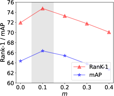
(a)

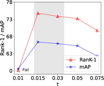
(b)

Figure 3: Variation of performance with different $m$ and $\tau$.

Robustness Study

In this section, we provide some visualization results during cross-modal training to verify the robustness and effectiveness of our method. As shown in Figure 4, one can clearly see that our RDE not only achieves excellent performance under noise but also effectively alleviates noise overfitting.

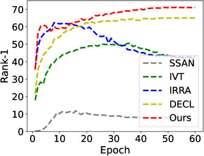
(a)

(b)

Figure 4: Test performance (Rank-1) versus epochs on CHUK-PEDES and ICFG-PEDES datasets with 50% noise.

Conclusion

In this paper, we reveal and study a novel challenging problem of noisy correspondence (NC) in TIReID, which violates the common assumption of existing methods that image-text data is perfectly aligned. To this end, we propose a robust method, i.e., RDE, to effectively handle the revealed NC problem and achieve superior performance. Extensive experiments are conducted on three benchmark datasets to comprehensively demonstrate the superiority and robustness of our method both with and without synthetic NCs.

In this supplementary material, we provide additional information for RDE. More specifically, we first give a detailed proof for Lemma 2 in section A. In section B, we detail the used datasets and the compared baselines. In section C, to further verify the robustness of RDE, we provide the re-identification performance on three benchmark datasets under extremely high noise rate, i.e., 80%. Besides, in section D, we provide more comparison results compared with state-of-art methods to comprehensively verify the superiority of our RDE. In section E, we explore the impact of different selection ratios ($\mathcal{R}$) on performance. In section F, we provide a targeted ablation analysis for TSE. In section G, we provide a large number of real noisy examples existing in the three public datasets to conduct a case study, thus emphasizing our motivation. We also provide a more comprehensive robustness analysis to verify the robustness of RDE in section H. Finally, in section I, we provide some qualitative results to illustrate the advantages of our RDE.

A. Proof for Lemma 2

Given an input image-text pair $(I_{i},T_{i})$ in a mini-batch $\mathbf{x}$, TAL is defined as:

where $m$ is a positive margin coefficient, $\tau$ is a temperature coefficient to control hardness, $S(I_{i},T_{j})\in\{S_{ij}^{b},S_{ij}^{e}\}$, $[x]_{+}\equiv\max(x,0)$, $q_{ij}=1-l_{ij}$, and $K$ is the size of $\mathbf{x}$. Since multiple positive pairs from the same identity may appear in the mini-batch, $S^{+}_{i2t}(I_{i})=\sum^{K}_{j=1}\alpha_{ij}S(I_{i},T_{j})$ is the weighted mean similarity of positive pairs for image $I_{i}$, where $\alpha_{ij}=\frac{l_{ij}\exp{(S(I_{i},T_{j})/\tau)}}{\sum^{N}_{k=1}l_{ik}\exp{(S(I_{i},T_{k})/\tau)}}$. And, $S^{+}_{i2t}(T_{i})$ is similar to the definition of $S^{+}_{i2t}(I_{i})$.

Lemma 2.

TAL is the upper bound of TRL, i.e.,

$$\mathcal{L}_{trl}(I_{i},T_{i})=\big{[}m-S^{+}_{i2t}(I_{i})+S(I_{i},\hat{T}_{i})\big{]}_{+}$$ (9)

$$+\big{[}m-S^{+}_{t2i}(T_{i})+S(\hat{I}_{i},T_{i})\big{]}_{+}\leq\mathcal{L}_{tal}(I_{i},T_{i}),$$

where $\hat{T}_{i}\in\mathbf{T}_{i}=\{T_{j}|l_{ij}=0,\forall j\in\{1,2,\cdots,K\}\}$ is the hardest negative text for image $I_{i}$ and $\hat{I}_{i}\in\mathbf{I}_{i}=\{I_{j}|l_{ji}=0,\forall j\in\{1,2,\cdots,K\}\}$ is the hardest negative image for text $I_{i}$, respectively.

Proof.

To prove Equation 9, we first take the image-to-text direction as an example. For $S(I_{i},\hat{T}_{i})$ in Equation 9, we have that

$$S(I_{i},\hat{T}_{i}) =\max_{T_{j}\in\mathbf{T}_{i}}\left(S(I_{i},T_{j})\right)$$ (10)

$$=\max_{T_{j}\in\mathbf{T}_{i}}\left(\tau\log\exp\left(S(I_{i},T_{j})\right)^{\frac{1}{\tau}}\right)$$

$$=\tau\log\left(\max_{T_{j}\in\mathbf{T}_{i}}\left(\exp\left(S(I_{i},T_{j})\right)^{\frac{1}{\tau}}\right)\right)$$

$$\leq\tau\log\left(\sum_{T_{j}\in\mathbf{T}_{i}}\exp(S(I_{i},T_{j})/\tau)\right)$$

$$\leq\tau\log(\sum_{j=1}^{K}q_{ij}\exp(S(I_{i},T_{j})/\tau)),$$

where $q_{ij}=1-l_{ij}$. Based on Equation 10, we have that

$$\begin{gathered}\big{[}m-S^{+}_{i2t}(I_{i})+\tau\log(\sum_{j=1}^{K}q_{ij}\exp(S(I_{i},T_{j})/\tau))\big{]}_{+}\\ \geq\big{[}m-S^{+}_{i2t}(I_{i})+S(I_{i},\hat{T}_{i})\big{]}_{+}.\end{gathered}$$ (11)

Similarly, in the text-to-image direction, we have that

$$\begin{gathered}\big{[}m-S^{+}_{t2i}(T_{i})+\tau\log(\sum_{j=1}^{K}q_{ji}\exp(S(I_{j},T_{i})/\tau))\big{]}_{+}\\ \geq\big{[}m-S^{+}_{t2i}(T_{i})+S(\hat{I}_{i},T_{i})\big{]}_{+}.\end{gathered}$$ (12)

Thus, combining Equation 11 and Equation 12, we can get $\mathcal{L}_{trl}(I_{i},T_{i})\leq\mathcal{L}_{tal}(I_{i},T_{i})$. This completes the proof. ∎

B. Dataset and Baseline Description

Datasets.

To verify the effectiveness and superiority of RDE, we use three widely-used image-text person datasets to conduct experiments. A brief introduction of these datasets is given as follows:

• CHUK-PEDES (Li et al. 2017) is the first large-scale benchmark to dedicate TIReID, which includes 40,206 person images and 80,412 text descriptions for 13,003 unique identities. We follow the official data split to conduct experiments, i.e., 11,003 identities for training, 1,000 identities for validation, and the rest of the 1,000 identities for testing.

• ICFG-PEDES (Ding et al. 2021) is a widely-used benchmark collected from the MSMT17 dataset (Wei et al. 2018) and consists of 54,522 images for 4,102 unique persons and each image has a corresponding textual description. We follow the data split used by most TIReID methods (Shu et al. 2022; Jiang and Ye 2023), i.e., a training set with 3,102 identifies and a validation set with 1,000 identifies. Note that we uniformly used the validation performance as the test performance due to its lack of a test set.

• RSTPReid (Zhu et al. 2021) is another benchmark dataset constructed from the MSMT17 dataset (Wei et al. 2018) for TIReID. RSTPReid contains 20,505 images for 4,101 identities, wherein each person has 5 images and each image is paired with 2 text descriptions. Following the official data split, we use 3,701 identities for training, 200 identities for validation, and the remaining 200 identities for testing.

Baselines.

To verify the effectiveness and robustness of our method in the NC scenario, we provide the comparison results with 5 baselines that have published code. We introduce each baseline as follows:

• SSAN (Ding et al. 2021) is a local-matching method for TIReID, which mainly benefits from a proposed multiview non-local network that could capture the local relationships, thus establishing better correspondences between body parts and noun phrases. Besides, SSAN also exploits a compound ranking loss to make an effective reduction of the intra-class variance in textual features.

• IVT (Shu et al. 2022) is an implicit visual-textual framework, which belongs to the global-matching method. To explore fine-grained alignments, IVT utilizes two implicit semantic alignment paradigms, i.e., multi-level alignment (MLA) and bidirectional mask modeling (BMM). MLA aims to see “finer” by exploring local and global alignments from three-level matchings. BMM aims to see “more” by mining more semantic alignments from random masking for both modalities.

• IRRA (Jiang and Ye 2023) is a recent state-of-art global-matching method that could learn relations between local visual-textual tokens and enhances global alignments without requiring additional prior supervision. IRRA exploits a novel similarity distribution matching to minimize the KL divergence between the similarity distributions and the normalized label matching distributions for better performance.

• CLIP-C is a quite strong baseline that fine-tunes the original CLIP model with only clean image-text pairs. We use the same version as IRRA, i.e., ViTB/16, for a fair comparison and use InfoNCE loss (Oord, Li, and Vinyals 2018) to optimize the model.

• DECL (Qin et al. 2022) is an effective robust image-text matching framework, which utilizes the cross-modal evidential learning paradigm to capture and leverage the uncertainty brought by noise to isolate the noisy pairs. Since TIReID can be treated as the sub-task of instance-level image-text matching, DECL also can be used to ease the negative impact of NCs in TIReID. In this paper, we exploit the used model of IRRA (Jiang and Ye 2023) as the base model of DECL for robust TIReID.

			CUHK-PEDES					ICFG-PEDES					RSTPReid
Noise	Methods		R-1	R-5	R-10	mAP	mINP	R-1	R-5	R-10	mAP	mINP	R-1	R-5	R-10	mAP	mINP
80%	SSAN	Best	0.18	0.83	1.45	0.47	0.24	0.28	0.99	1.90	0.27	0.15	0.65	3.25	5.95	1.30	0.70
		Last	0.13	0.67	1.46	0.42	0.21	0.18	1.01	1.77	0.25	0.14	0.65	2.95	5.85	1.32	0.68
	IVT	Best	34.03	55.49	66.16	33.90	23.29	21.10	37.10	45.64	13.68	2.32	15.15	30.00	40.50	14.98	7.79
		Last	10.61	23.81	31.38	11.13	5.72	5.64	12.48	17.15	4.00	0.69	4.95	13.55	19.75	6.07	2.85
	IRRA	Best	38.63	56.69	64.18	34.60	21.84	28.19	44.14	51.27	14.36	1.41	29.65	46.65	54.50	23.77	11.32
		Last	9.06	19.69	25.65	8.26	3.18	8.68	18.76	24.50	3.65	0.27	8.15	21.00	29.05	7.28	2.40
	CLIP-C	Best	57.38	78.05	84.97	51.08	34.83	44.84	65.24	73.27	24.27	3.42	47.80	72.70	81.75	37.50	18.09
		Last	57.05	78.09	85.07	51.14	35.05	44.65	65.26	73.45	24.20	3.44	44.60	70.75	80.20	35.67	17.09
	DECL	Best	47.90	71.57	80.17	44.51	29.86	40.53	61.49	69.84	21.78	2.97	48.15	72.20	80.75	37.31	18.83
		Last	46.57	70.19	78.48	42.93	27.91	39.91	61.16	69.51	21.56	2.89	45.85	71.05	81.00	35.34	16.35
	RDE	Best	64.94	83.11	89.08	57.57	40.77	50.79	70.08	77.59	26.44	3.36	51.65	75.55	84.20	39.06	18.53
		Last	65.11	83.19	89.12	57.72	40.93	50.75	70.05	77.53	26.44	3.36	45.05	71.20	80.15	33.91	14.29

Table 3: Performance comparison under 80% noise rate on three benchmarks. “Best” means choosing the best checkpoint on the validation set to test, and “Lest” stand for choosing the checkpoint after the last training epoch to conduct inference. R-1,5,10 is an abbreviation for Rank-1,5,10 (%) accuracy. The best and second-best results are in bold and underline, respectively.

C. The Results under Extreme Noise

To further verify the effectiveness and robustness of our method, we report comparison results under extremely high noise, i.e., 80%. From the results in Table 3, one can see that our RDE achieves the best performance and can effectively alleviate the performance degradation caused by noise overfitting. For example, compare with the ‘Best’ rows, our RDE surpasses the best baselines by +7.56%, +5.95%, and +3.5% in terms of Rank-1 on the three datasets, respectively.

Methods	Ref.	Image Enc.	Text Enc.	R-1	R-5	R-10	mAP	mINP
CMPM/C (Zhang and Lu 2018)	ECCV’18	RN50	LSTM	49.37	-	79.27	-	-
TIMAM (Sarafianos, Xu, and Kakadiaris 2019)	ICCV’19	RN101	BERT	54.51	77.56	79.27	-	-
ViTAA (Wang et al. 2020)	ECCV’20	RN50	LSTM	54.92	75.18	82.90	51.60	-
NAFS (Gao et al. 2021)	arXiv’21	RN50	BERT	59.36	79.13	86.00	54.07	-
DSSL (Zhu et al. 2021)	MM’21	RN50	BERT	59.98	80.41	87.56	-	-
SSAN (Ding et al. 2021)	arXiv’21	RN50	LSTM	61.37	80.15	86.73		-
Lapscore (Wu et al. 2021)	ICCV’21	RN50	BERT	63.4	-	87.80	-	-
ISANet (Yan et al. 2022b)	arXiv’22	RN50	LSTM	63.92	82.15	87.69	-	-
LBUL (Wang et al. 2022b)	MM’22	RN50	BERT	64.04	82.66	87.22	-	-
Han et al.2021	BMVC’21	CLIP-RN101	CLIP-Xformer	64.08	81.73	88.19	60.08	-
SAF (Li, Cao, and Zhang 2022)	ICASSP’22	ViT-Base	BERT	64.13	82.62	88.40	-	-
TIPCB (Chen et al. 2022)	Neuro’22	RN50	BERT	64.26	83.19	89.10	-	-
CAIBC (Wang et al. 2022a)	MM’22	RN50	BERT	64.43	82.87	88.37	-	-
AXM-Net (Farooq et al. 2022)	MM’22	RN50	BERT	64.44	80.52	86.77	58.73	-
LGUR (Shao et al. 2022)	MM’22	DeiT-Small	BERT	65.25	83.12	89.00	-	-
IVT (Shu et al. 2022)	ECCVW’22	ViT-Base	BERT	65.59	83.11	89.21	-	-
CFine (Yan et al. 2022a)	arXiv’22	CLIP-ViT	BERT	69.57	85.93	91.15	-	-
IRRA (Jiang and Ye 2023)	CVPR’23	CLIP-ViT	CLIP-Xformer	73.38	89.93	93.71	66.13	50.24
Our RDE	-	CLIP-ViT	CLIP-Xformer	75.94	90.63	94.04	67.92	51.74

Table 4: Performance comparisons on the CUHK-PEDES dataset. The best results are in bold.

D. More Comparisons

In this section, we follow the organization of IRRA (Jiang and Ye 2023) and provide more comparative experimental results on three benchmarks in Tables 4, 5 and 6. From the results, our RDE achieves the best results and exceeds the best baseline by a large margin, i.e., +2.56%, +4.14%, and +4.80% in terms of Rank-1 on three datasets, respectively.

Methods	R-1	R-5	R-10	mAP	mINP
Dual Path (Zheng et al. 2020)	38.99	59.44	68.41	-	-
CMPM/C (Zhang and Lu 2018)	43.51	65.44	74.26	-	-
ViTAA (Wang et al. 2020)	50.98	68.79	75.78	-	-
SSAN (Ding et al. 2021)	54.23	72.63	79.53	-	-
IVT (Shu et al. 2022)	56.04	73.60	80.22	-	-
ISANet (Yan et al. 2022b)	57.73	75.42	81.72	-	-
CFine (Yan et al. 2022a)	60.83	76.55	82.42	-	-
IRRA (Jiang and Ye 2023)	63.46	80.25	85.82	38.06	7.93
Our RDE	67.60	82.47	87.17	40.34	8.01

Table 5: Performance comparisons on the ICFG-PEDES dataset. The best results are in bold.

Methods	R-1	R-5	R-10	mAP	mINP
DSSL (Zhu et al. 2021)	39.05	62.60	73.95	-	-
SSAN (Ding et al. 2021)	43.50	67.80	77.15	-	-
LBUL (Wang et al. 2022b)	45.55	68.20	77.85	-	-
IVT (Shu et al. 2022)	46.70	70.00	78.80	-	-
CFine (Yan et al. 2022a)	50.55	72.50	81.60	-	-
IRRA (Jiang and Ye 2023)	60.20	81.30	88.20	47.17	25.28
Our RDE	65.00	84.75	90.60	51.57	28.99

Table 6: Performance comparisons on the RSTPReid dataset. The best results are in bold.

E. The impact of $\mathcal{R}$

Figure 5 shows the variation of performance with different $\mathcal{R}$. From the figure, one can see that too large or too small R will cause suboptimal performance. We think that a small $R$ will cause too much information loss and learn poor embedding presentations, while too large will focus on too many meaningless features. For this reason, we recommend $\mathcal{R}$ to be set between 0.3$\sim$0.5. In all experiments, $\mathcal{R}$ is set to 0.3.

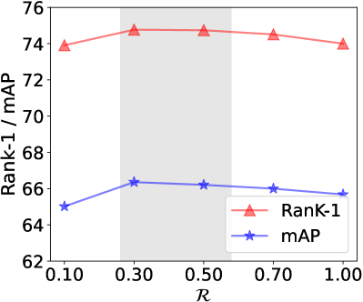
(a)

(b)

Figure 5: Variation of performance with different $\mathcal{R}\in[0,1]$

F. Ablation analysis for TSE

To verify the design rationality of TSE in our RDE, we conduct dedicated ablation experiments on TSE. The results are reported in Table 7. In the table, TSE^′ means that the token features encoded by CLIP are directly used for aggregation to obtain the embedding representations instead of conducting embedding transformation. Also, we show the impact of different pooling strategies on performance. From the results, our standard version of TSE obtains the best performance, i.e., conducting the embedding transformation and using the max-pooling strategy to obtain the TSE representations.

Methods	Pool	R-1	R-5	R-10	mAP	mINP
TSE′	Avg.	67.22	84.96	90.03	60.22	43.84
TSE′	TopK.	67.72	85.72	90.98	60.59	43.95
TSE′	Max.	67.25	84.76	90.29	59.45	42.50
TSE	Avg.	67.17	85.10	90.51	60.20	44.15
TSE	TopK.	69.90	86.74	91.41	62.35	45.87
TSE	Max.	71.00	87.98	92.50	63.51	47.03

Table 7: Performance comparisons with state-of-the-art methods on the RSTPReid dataset. ’Avg.’, ’TopK.’, and ’Max.’ indicate the use of average-pooling, topK-pooling (K=10), and max-pooling strategies, respectively.

G. Case Study

In this section, we show a large number of real examples of noisy pairs in three public datasets without synthetic NCs in Figures 6, 7 and 8, which are identified by CCD. Note that for privacy and security, the face areas of people in all images are blurred. From these examples, one can see that there are various reasons for noisy correspondences, e.g., occlusion (e.g., Figure 6(a,b)), lighting (e.g., Figure 6(c) and Figure 7(f)), and inaccurate noisy text descriptions (e.g., Figure 6(e,g) and Figure 8(a-f)). But all in all, these noisy pairs are real in these datasets and actually break the implicit assumption that all training image-text pairs are aligned correctly and perfectly at an instance level. Thus, we reveal the noisy correspondence problem in TIReID and propose a robust method, i.e., RDE, to particularly address it.

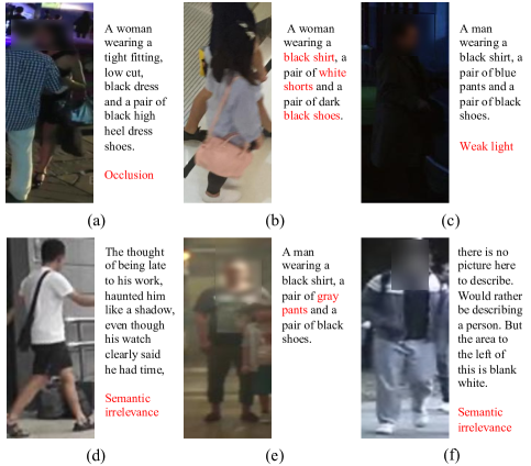
Figure 6: The examples of noisy correspondence identified by CCD on the CUHK-PEDES dataset.

H. Robustness Study

For a comprehensive robustness analysis, we provide more performance curves versus epochs in Figures 9, 10 and 11. It can be seen from the Figure 9 that when the noise rate is 20%, each baseline shows a certain degree of robustness, and there is no obvious performance degradation due to over-fitting noisy pairs. However, as the noise rate increases, the non-robust methods (SSAN, IVT, and IRRA) all show a curve that first rises and then falls. This tendency is caused by the memorization effect that DNNs tend to learn simple patterns before fitting noisy samples. Besides, we can also find that when the noise rate is 80%, SSAN fails and other non-robust methods (IVT and IRRA) also have a serious performance drop. By contrast, thanks to the CCD and TAL, our RDE can learn accurate visual-semantic associations by obtaining confident clean training image-text pairs, which can effectively and directly prevent over-fitting noisy pairs, thus achieving robust cross-modal learning. From these figures, our method not only exhibits strong robustness but also achieves excellent re-identification performance.

Figure 7: The examples of noisy correspondence identified by CCD on the ICFG-PEDES dataset.

Figure 8: The examples of noisy correspondence identified by CCD on the RSTPReid dataset.

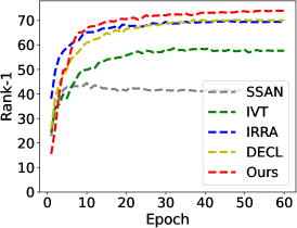
(a)

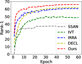
(b)

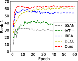
(c)

Figure 9: Test performance (Rank-1) versus epochs on three datasets with 20% noise.

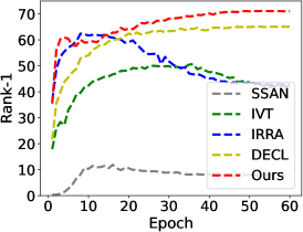
(a)

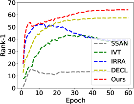
(b)

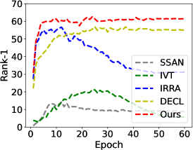
(c)

Figure 10: Test performance (Rank-1) versus epochs on three datasets with 50% noise.

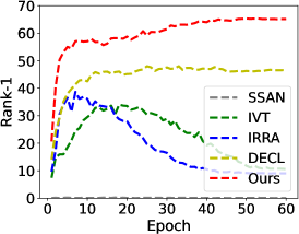
(a)

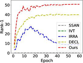
(b)

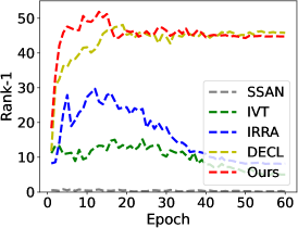
(c)

Figure 11: Test performance (Rank-1) versus epochs on three datasets with 80% noise.

I. Qualitative Results

To illustrate the advantages of our RDE, some retrieved examples for TIReID are presented in Figure 12. These results are obtained by testing the model trained on the CUHK-PEDES dataset with 20% NCs. From the examples, one can see that our RDE obtains more accurate and reasonable re-identification results. Simultaneously, in some inaccurate results (e.g., the results (b) and (d)) obtained by IRRA, we find that the visual information of the retrieved image often only matches part of the text query, which indicates that the model cannot learn complete alignment knowledge. We think the reason is that the NCs mislead the model of IRRA to focus on some wrong visual-semantic associations. In contrast, our RDE could filter out erroneous correspondences to learn reliable and accurate cross-modal knowledge, thus achieving high robustness and better results.

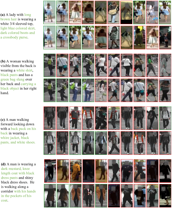
Figure 12: Comparison of top-10 retrieved results on the CUHK-PEDES dataset between the baseline IRRA (the first row) and our RDE (the second row) for each text query. The matched and mismatched person images are marked with red and blue rectangles, respectively. All face areas of people in images are blurred for privacy and security.

References

- Arpit et al. (2017) Arpit, D.; Jastrzȩbski, S.; Ballas, N.; Krueger, D.; Bengio, E.; Kanwal, M. S.; Maharaj, T.; Fischer, A.; Courville, A.; Bengio, Y.; and Lacoste-Julien, S. 2017. A Closer Look at Memorization in Deep Networks. In Precup, D.; and Teh, Y. W., eds., Proceedings of the 34th International Conference on Machine Learning, volume 70 of Proceedings of Machine Learning Research, 233–242. PMLR.
- Chen et al. (2022) Chen, Y.; Zhang, G.; Lu, Y.; Wang, Z.; and Zheng, Y. 2022. Tipcb: A simple but effective part-based convolutional baseline for text-based person search. Neurocomputing, 494: 171–181.
- Devlin et al. (2018) Devlin, J.; Chang, M.-W.; Lee, K.; and Toutanova, K. 2018. Bert: Pre-training of deep bidirectional transformers for language understanding. arXiv preprint arXiv:1810.04805.
- Diao et al. (2021) Diao, H.; Zhang, Y.; Ma, L.; and Lu, H. 2021. Similarity reasoning and filtration for image-text matching. In Proceedings of the AAAI Conference on Artificial Intelligence, volume 35, 1218–1226.
- Ding et al. (2021) Ding, Z.; Ding, C.; Shao, Z.; and Tao, D. 2021. Semantically self-aligned network for text-to-image part-aware person re-identification. arXiv preprint arXiv:2107.12666.
- Dong et al. (2021) Dong, J.; Li, X.; Xu, C.; Yang, X.; Yang, G.; Wang, X.; and Wang, M. 2021. Dual encoding for video retrieval by text. IEEE Transactions on Pattern Analysis and Machine Intelligence, 44(8): 4065–4080.
- Dosovitskiy et al. (2020) Dosovitskiy, A.; Beyer, L.; Kolesnikov, A.; Weissenborn, D.; Zhai, X.; Unterthiner, T.; Dehghani, M.; Minderer, M.; Heigold, G.; Gelly, S.; et al. 2020. An image is worth 16x16 words: Transformers for image recognition at scale. arXiv preprint arXiv:2010.11929.
- Eom and Ham (2019) Eom, C.; and Ham, B. 2019. Learning disentangled representation for robust person re-identification. Advances in neural information processing systems, 32.
- Faghri et al. (2017) Faghri, F.; Fleet, D. J.; Kiros, J. R.; and Fidler, S. 2017. Vse++: Improving visual-semantic embeddings with hard negatives. arXiv preprint arXiv:1707.05612.
- Farooq et al. (2022) Farooq, A.; Awais, M.; Kittler, J.; and Khalid, S. S. 2022. AXM-Net: Implicit cross-modal feature alignment for person re-identification. In Proceedings of the AAAI Conference on Artificial Intelligence, volume 36, 4477–4485.
- Feng et al. (2023) Feng, Y.; Zhu, H.; Peng, D.; Peng, X.; and Hu, P. 2023. RONO: Robust Discriminative Learning With Noisy Labels for 2D-3D Cross-Modal Retrieval. In Proceedings of the IEEE/CVF Conference on Computer Vision and Pattern Recognition (CVPR), 11610–11619.
- Gao et al. (2021) Gao, C.; Cai, G.; Jiang, X.; Zheng, F.; Zhang, J.; Gong, Y.; Peng, P.; Guo, X.; and Sun, X. 2021. Contextual non-local alignment over full-scale representation for text-based person search. arXiv preprint arXiv:2101.03036.
- Han et al. (2018) Han, B.; Yao, Q.; Yu, X.; Niu, G.; Xu, M.; Hu, W.; Tsang, I.; and Sugiyama, M. 2018. Co-teaching: Robust training of deep neural networks with extremely noisy labels. Advances in neural information processing systems, 31.
- Han et al. (2023) Han, H.; Miao, K.; Zheng, Q.; and Luo, M. 2023. Noisy Correspondence Learning with Meta Similarity Correction. In Proceedings of the IEEE/CVF Conference on Computer Vision and Pattern Recognition, 7517–7526.
- Han et al. (2021) Han, X.; He, S.; Zhang, L.; and Xiang, T. 2021. Text-based person search with limited data. arXiv preprint arXiv:2110.10807.
- He et al. (2016) He, K.; Zhang, X.; Ren, S.; and Sun, J. 2016. Deep residual learning for image recognition. In Proceedings of the IEEE conference on computer vision and pattern recognition, 770–778.
- Hu et al. (2023) Hu, P.; Huang, Z.; Peng, D.; Wang, X.; and Peng, X. 2023. Cross-Modal Retrieval with Partially Mismatched Pairs. IEEE Transactions on Pattern Analysis and Machine Intelligence, 1–15.
- Huang et al. (2021) Huang, Z.; Niu, G.; Liu, X.; Ding, W.; Xiao, X.; Wu, H.; and Peng, X. 2021. Learning with noisy correspondence for cross-modal matching. Advances in Neural Information Processing Systems, 34: 29406–29419.
- Jiang and Ye (2023) Jiang, D.; and Ye, M. 2023. Cross-Modal Implicit Relation Reasoning and Aligning for Text-to-Image Person Retrieval. In Proceedings of the IEEE/CVF Conference on Computer Vision and Pattern Recognition, 2787–2797.
- Jing et al. (2020) Jing, Y.; Si, C.; Wang, J.; Wang, W.; Wang, L.; and Tan, T. 2020. Pose-guided multi-granularity attention network for text-based person search. In Proceedings of the AAAI Conference on Artificial Intelligence, volume 34, 11189–11196.
- Li, Socher, and Hoi (2020) Li, J.; Socher, R.; and Hoi, S. C. 2020. Dividemix: Learning with noisy labels as semi-supervised learning. arXiv preprint arXiv:2002.07394.
- Li, Cao, and Zhang (2022) Li, S.; Cao, M.; and Zhang, M. 2022. Learning semantic-aligned feature representation for text-based person search. In ICASSP 2022-2022 IEEE International Conference on Acoustics, Speech and Signal Processing (ICASSP), 2724–2728. IEEE.
- Li et al. (2017) Li, S.; Xiao, T.; Li, H.; Zhou, B.; Yue, D.; and Wang, X. 2017. Person search with natural language description. In Proceedings of the IEEE conference on computer vision and pattern recognition, 1970–1979.
- Lu, Bo, and He (2022) Lu, Y.; Bo, Y.; and He, W. 2022. An Ensemble Model for Combating Label Noise. In Proceedings of the Fifteenth ACM International Conference on Web Search and Data Mining, 608–617.
- Niu et al. (2020) Niu, K.; Huang, Y.; Ouyang, W.; and Wang, L. 2020. Improving description-based person re-identification by multi-granularity image-text alignments. IEEE Transactions on Image Processing, 29: 5542–5556.
- Oord, Li, and Vinyals (2018) Oord, A. v. d.; Li, Y.; and Vinyals, O. 2018. Representation learning with contrastive predictive coding. arXiv preprint arXiv:1807.03748.
- Qin et al. (2022) Qin, Y.; Peng, D.; Peng, X.; Wang, X.; and Hu, P. 2022. Deep evidential learning with noisy correspondence for cross-modal retrieval. In Proceedings of the 30th ACM International Conference on Multimedia, 4948–4956.
- Radford et al. (2021) Radford, A.; Kim, J. W.; Hallacy, C.; Ramesh, A.; Goh, G.; Agarwal, S.; Sastry, G.; Askell, A.; Mishkin, P.; Clark, J.; et al. 2021. Learning transferable visual models from natural language supervision. In International conference on machine learning, 8748–8763. PMLR.
- Sarafianos, Xu, and Kakadiaris (2019) Sarafianos, N.; Xu, X.; and Kakadiaris, I. A. 2019. Adversarial representation learning for text-to-image matching. In Proceedings of the IEEE/CVF international conference on computer vision, 5814–5824.
- Shao et al. (2022) Shao, Z.; Zhang, X.; Fang, M.; Lin, Z.; Wang, J.; and Ding, C. 2022. Learning Granularity-Unified Representations for Text-to-Image Person Re-identification. In Proceedings of the 30th ACM International Conference on Multimedia.
- Shu et al. (2022) Shu, X.; Wen, W.; Wu, H.; Chen, K.; Song, Y.; Qiao, R.; Ren, B.; and Wang, X. 2022. See finer, see more: Implicit modality alignment for text-based person retrieval. In European Conference on Computer Vision, 624–641. Springer.
- Wang et al. (2021) Wang, C.; Luo, Z.; Lin, Y.; and Li, S. 2021. Text-based Person Search via Multi-Granularity Embedding Learning. In IJCAI, 1068–1074.
- Wang et al. (2020) Wang, Z.; Fang, Z.; Wang, J.; and Yang, Y. 2020. Vitaa: Visual-textual attributes alignment in person search by natural language. In Computer Vision–ECCV 2020: 16th European Conference, Glasgow, UK, August 23–28, 2020, Proceedings, Part XII 16, 402–420. Springer.
- Wang et al. (2015) Wang, Z.; Hu, R.; Yu, Y.; Liang, C.; and Huang, W. 2015. Multi-level fusion for person re-identification with incomplete marks. In Proceedings of the 23rd ACM international conference on Multimedia, 1267–1270.
- Wang et al. (2022a) Wang, Z.; Zhu, A.; Xue, J.; Wan, X.; Liu, C.; Wang, T.; and Li, Y. 2022a. Caibc: Capturing all-round information beyond color for text-based person retrieval. In Proceedings of the 30th ACM International Conference on Multimedia, 5314–5322.
- Wang et al. (2022b) Wang, Z.; Zhu, A.; Xue, J.; Wan, X.; Liu, C.; Wang, T.; and Li, Y. 2022b. Look before you leap: Improving text-based person retrieval by learning a consistent cross-modal common manifold. In Proceedings of the 30th ACM International Conference on Multimedia, 1984–1992.
- Wei et al. (2018) Wei, L.; Zhang, S.; Gao, W.; and Tian, Q. 2018. Person transfer gan to bridge domain gap for person re-identification. In Proceedings of the IEEE conference on computer vision and pattern recognition, 79–88.
- Wu et al. (2021) Wu, Y.; Yan, Z.; Han, X.; Li, G.; Zou, C.; and Cui, S. 2021. LapsCore: language-guided person search via color reasoning. In Proceedings of the IEEE/CVF International Conference on Computer Vision, 1624–1633.
- Yan et al. (2022a) Yan, S.; Dong, N.; Zhang, L.; and Tang, J. 2022a. Clip-driven fine-grained text-image person re-identification. arXiv preprint arXiv:2210.10276.
- Yan et al. (2022b) Yan, S.; Tang, H.; Zhang, L.; and Tang, J. 2022b. Image-specific information suppression and implicit local alignment for text-based person search. arXiv preprint arXiv:2208.14365.
- Yang et al. (2022) Yang, M.; Huang, Z.; Hu, P.; Li, T.; Lv, J.; and Peng, X. 2022. Learning with twin noisy labels for visible-infrared person re-identification. In Proceedings of the IEEE/CVF conference on computer vision and pattern recognition, 14308–14317.
- Zhang et al. (2023) Zhang, H.; Yang, Y.; Qi, F.; Qian, S.; and Xu, C. 2023. Robust Video-Text Retrieval via Noisy Pair Calibration. IEEE Transactions on Multimedia.
- Zhang and Lu (2018) Zhang, Y.; and Lu, H. 2018. Deep cross-modal projection learning for image-text matching. In Proceedings of the European conference on computer vision (ECCV), 686–701.
- Zheng et al. (2020) Zheng, Z.; Zheng, L.; Garrett, M.; Yang, Y.; Xu, M.; and Shen, Y.-D. 2020. Dual-path convolutional image-text embeddings with instance loss. ACM Transactions on Multimedia Computing, Communications, and Applications (TOMM), 16(2): 1–23.
- Zhu et al. (2021) Zhu, A.; Wang, Z.; Li, Y.; Wan, X.; Jin, J.; Wang, T.; Hu, F.; and Hua, G. 2021. Dssl: Deep surroundings-person separation learning for text-based person retrieval. In Proceedings of the 29th ACM International Conference on Multimedia, 209–217.
- Zhu et al. (2022) Zhu, H.; Ke, W.; Li, D.; Liu, J.; Tian, L.; and Shan, Y. 2022. Dual cross-attention learning for fine-grained visual categorization and object re-identification. In Proceedings of the IEEE/CVF Conference on Computer Vision and Pattern Recognition, 4692–4702.