Utilizing Semantic Textual Similarity for Clinical Survey Data Feature Selection

Abstract

Survey data can contain a high number of features while having a comparatively low quantity of examples. Machine learning models that attempt to predict outcomes from survey data under these conditions can overfit and result in poor generalizability. One remedy to this issue is feature selection, which attempts to select an optimal subset of features to learn upon. A relatively unexplored source of information in the feature selection process is the usage of textual names of features, which may be semantically indicative of which features are relevant to a target outcome. The relationships between feature names and target names can be evaluated using language models (LMs) to produce semantic textual similarity (STS) scores, which can then be used to select features. We examine the performance using STS to select features directly and in the minimal-redundancy-maximal-relevance (mRMR)algorithm. The performance of STS as a feature selection metric is evaluated against preliminary survey data collected as a part of a clinical study on persistent post-surgical pain (PPSP). The results suggest that features selected with STS can result in higher performance models compared to traditional feature selection algorithms.

Introduction

Because of the high cost of collecting surveys in human subjects research, survey data can suffer from high dimensionality and an relatively inadequate number of examples to learn from. One solution is to select a subset of features when training an ML model, but because this relies upon the already small data to learn from, suboptimal selections can be made. This issue is particularly important for clinical data, where the true relationships between features and labels may be too complex or unknown to make optimal decisions regarding feature choices. We explore this problem through a collection of surveys collected to assess persistent post-surgical pain (PPSP), where a patient experiences surgically-related pain for longer than expected (Vila et al. 2020), and whose exact causes are presently unclear (Haroutiunian et al. 2013).

Proposed Approach

Survey answers are the result of questions that have text that may be semantically related to a target outcome, and in turn semantically similar or dissimilar to one another. Intuition suggests that STS is a useful analogue to statistical measures that capture relationships between features, such as mutual information (MI). STS may then be useful for determining which questions are relevant to predicting a target question. Moreover, STS scores may be useful in determining which questions are redundant to each other. This may be especially helpful for smaller datasets where there is a limited amount of information immediately available to learn from. To this end, we evaluate the use of STS scores directly to determine the most relevant features, and test STS scores both as a direct replacement and compliment in algorithms utilizing statistical scores, such as minimal-redundancy-maximal-relevance (mRMR).

There appears to be nearly no literature examining feature selection with embeddings or STS. The closest match to our knowledge examined the usage of word2vec continuous bag-of-words embeddings (Mikolov et al. 2013) trained upon Twitter data to select Google search query trends matching the embeddings of a target concept (Lampos, Zou, and Cox 2017). Our analysis differs in several key ways, with the principal difference being that we evaluate selection using the top $N$ STS scores and mRMR, in addition to the procedure in Lampos, Zou, and Cox (2017), where they features select beyond a $k$-standard deviation threshold. Another major difference is the usage of large language models (LLMs) to calculate scores, which is a more recent model than word2vec, and demonstrably perform better with regards to general and clinical tasks (Roy and Pan 2021). Finally, Lampos, Zou, and Cox (2017) apply their filtration method to a dataset with 35,572 different time-series features, whereas we evaluate a smaller tabular dataset in both examples and dimensions.

We present several empirical contributions in this paper:

• An examination of how STS scores generated by LMs between feature and target questions can help select features, either alone or in combination with statistical measures such as MI.

• Evaluating the performance of STS scores produced by different models in feature selection.

• A demonstration of how STS-based feature selection algorithms can reduce overfitting.

We make our code available at https://github.com/bcwarner/sts-select, and via pip install sts-select.

Related Work

Feature Selection

Fitting high-dimensional data is particularly difficult when the number of examples is low—as is with clinical data collected from human subjects—since a model can easily overfit on the training data. To counter this, we can employ the strategy of feature selection, where a subset of the overall features in a dataset are selected for learning.

Feature selection methods can be divided into three categories: embedded, wrapper, and filter methods. Embedded methods incorporate feature selection as a part of training, while wrapper methods interact in a feedback loop with the learning model. Filter methods select a subset of features based on properties of the dataset before the model is able to learn on the dataset, which differs from embedded and wrapper methods in that they do not form a feedback loop with the model (Guyon et al. 2008). Because of their independence, they tend to generalize well (Remeseiro and Bolon-Canedo 2019).

Feature selection methods used in clinical survey data cover a broad range of techniques. A study examining autism spectrum disorder (ASD) survey data, examined feature selection using principal component analysis, t-distributed stochastic neighbor embedding, and denoising autoencoders; and also found that survey features targeting ASD tend to have high levels of redundancy (Washington et al. 2019). Some of the other feature selection methods found for models involve questionnaires include wrapper models based on random forests (Niemann et al. 2020), bootstrapped feature selection (Abbas et al. 2018), principal component analysis, multicluster feature selection (Saridewi and Sari 2020), permutation importance (Chen, Wang, and Lu 2023), and ReliefF (Abut, Akay, and George 2016).

One particularly useful feature selection technique for is minimal-redundancy-maximal-relevance (mRMR), which aims to maximize the relevance of features to the target, while minimizing the redundancy between selected features. This is particularly useful when we have a small number of features that are correlated and want to ensure a model incorporates as broad as a set of information as possible (Peng, Long, and Ding 2005; Ramírez-Gallego et al. 2017).

Underpinning the mRMR objective function is the mutual information (MI)between classes and features, which measures the amount of shared information between two distributions.

Calculating true MI between two features is computationally costly, but can be approximated using one of several methods. The MI approximation methods used in this paper are from scikit-learn (Pedregosa et al. 2011), and are a synthesis of the $k$-nearest neighbors approaches described in (Kraskov, Stögbauer, and Grassberger 2004; Ross 2014).

Semantic textual similarity

Semantic textual similarity (STS)is a task where a LM is used to score the semantic similarity of two sentences, generally by evaluating the differences between embeddings generated by a model. Cosine similarity is one typical function used to compute the distance between embeddings (Reimers and Gurevych 2019; Oniani, Sivarajkumar, and Wang 2022).

STS scores can be produced with traditional LMs such as word2vec (Mikolov et al. 2013) or FastText (Joulin et al. 2016). They may also be produced with large language models (LLMs), which are a class of LM that is broadly defined as having on the order of high millions or more of parameters; and have been typically built with the transformer architecture (Manning 2022).

LLMs typically employ the pre-training/fine-tuning paradigm, where a model is trained with an unsupervised learning task, and then modified and trained to complete a supervised task (Devlin et al. 2018; Radford et al. 2019). Pre-training is particularly useful since it results in better generalization (Erhan et al. 2010), and because it means that computationally expensive pre-trained models can be reused for different tasks (Wolf et al. 2019). LLMs are distinct from traditional LMs in that they have demonstrated capabilities at many reasoning tasks involving semantic meaning (Singhal et al. 2022; Wei et al. 2023), and are highly applicable since survey features may involve more complex word relationships.

Clinical language involves vocabulary and semantic meaning that is often not present in non-clinical texts, and various pre-trained architectures exist to fill this gap. To date, there are over 80 clinical LMs available (Wornow et al. 2023), with a diverse set of architectural and training designs. Clinical LMs can perform better than general LMs on tasks specific to the clinical domain (Alsentzer et al. 2019), and can do so more efficiently than a general-purpose models (Lehman et al. 2023).

Methodology

Scoring & Selection

A distinction can be made between the scoring of features, where we measure a feature’s relationship to a target or another feature, and the selection of features, where we then use these scores to select the appropriate features. We evaluate the performance of two principal scoring tools, namely MI and STS. In addition, we evaluate the linear combination of them, with the coefficient for STS being a hyperparameter $\alpha$, which we test over a logarithmically-spaced range of 30 values from $[10^{-2},10^{2}]$. For selection methods that employ these scores, we evaluate selecting the top $N$ feature-target scores, selecting feature-target scores above a given standard deviation $k$, and selection with mRMR using these scores.

We restrict our analysis to filter methods because they because they are fit independently from the rest of the training pipeline, and as such do not have a feedback loop from which overfitting could occur (Remeseiro and Bolon-Canedo 2019), which are appropriate for small datasets. For all of the aforementioned selection algorithms, as well as the baseline algorithms we compare against, we select $20$ features since it is approximately an eighth of the features. For selection by standard deviations, all features with scores above $\mu+k\sigma$ are selected. We set $k=0.3$ for all Skipgram and FastText scorers due to low variance, and use $k=1$ for all others.

LMs and Fine-Tuning Datasets

For generating STS scores, we evaluate the performance of several different LLM, as well as Gensim’s (Řehůřek and Sojka 2010) implementation of Skipgram (Mikolov et al. 2013) and FastText (Joulin et al. 2016) for baseline comparisons. We use HuggingFace’s transformers (Wolf et al. 2019) with the sentence_transformers library (Reimers and Gurevych 2019) to fine-tune and produce STS scores. We evaluate two models trained on general vocabulary, namely all-MiniLM-L12-v2 (Reimers and Gurevych 2019), and bert-base-uncased (Devlin et al. 2018). We also evaluate the performance of models pre-trained on clinical/scientific text, including Bio_ClinicalBERT (Alsentzer et al. 2019), BioMed-RoBERTa-base (Gururangan et al. 2020), and PubMedBERT (Gu et al. 2021).

To fine-tune these models, we train the model to predict cosine similarity on one of two combined STS datasets, which we group into a general sentence-level and clinical phrase-level set. We also evaluate the performance of fine-tuning on both sets. Table 1 highlights the composition of the selected fine-tuning datsets.

Dataset	Type	Level	Examples
bio_simlex (Chiu et al. 2018)	Clinical	Phrase	987
bio_sim_verb (Chiu et al. 2018)	Clinical	Phrase	1,000
mayosrs (Pedersen et al. 2007)	Clinical	Phrase	101
Total Clinical			2,088
sts-companion (Cer et al. 2017)	General	Sentence	5,289
stsb_multi_mt;en (May 2021)	General	Sentence	5,749
Total General			11,038
Total			13,126

Table 1: Datasets used for training and fine-tuning selected models.

ClinicalSTS (Xiong et al. 2020) and MedSTS (Wang et al. 2020) are two clinical sentence-pair datasets, but we were unable to obtain them for fine-tuning. To overcome this limitation, we also evaluate the performance of a Bio_CinicalBERT model fine-tuned on just the ClinicalSTS dataset (Mulyar, Schumacher, and Dredze 2019).

Experiments

Data

The data is collected from a partially complete set of participants from the P5 - Personalized Prediction of Postsurgical Pain study (IRB #202101123) conducted at the Washington University/BJC Healthcare System.

A total of 12 surveys were assigned to individual users through the Research Electronic Data Capture (REDCap) system. The principal survey is the one described in Vila et al. (2020), which contains the four target outcome questions, and are described in more detail in Table 3. The other surveys include measures of psychological and physical pain, as well as correlated measures.

The dataset was assembled from REDCap on February 6th, 2023. It contains 1631 responses from a total 617 participants as a part of a final goal of 2,000 participants from the Anonymous Healthcare System. Table 2 outlines the key characteristics of the dataset, including number of examples and general demographics.

Name	Value
PPSP Characteristics
Individuals with Complete Mark	617
Responses by Individual (mean)	2.64
Responses by Individual (std. dev.)	1.54
Responses by Individual (max)	10
PPSP (+)	25
PPSP (-)	592
Race
Caucasian	497
American Indian / Alaskan Native	7
Asian	4
Black / African Heritage	98
Hawaiian Native / Other Pacific Islander	1
Other	9
Prefer not to answer	7
Sex Assigned at Birth
Female	425
Male	185
(No Answer)	7
Age
Age (min)	19
Age (mean)	52.4686
Age (std. dev.)	13.5219
Age (max)	75

Table 2: Demographics of the partial P5 dataset.

Data & Model Preparation

Several steps are taken to prepare the survey data for fitting upon the candidate models.

The first step taken is to prepare the label from this particular survey dataset. The label is derived from the four questions shown in Table 3 is determined using the binary formula $y_{1}=(Q_{1}\land Q_{2})\land(Q_{3}\geq 3\lor Q_{4}\geq 3)$. Once the labels are computed, these features are dropped from the dataset. Since we are attempting to predict PPSP, we filter out examples that where a column indicating six-month completion has a null value.

#	Question Text	Type
$y_{1}$	persistent_pain	T/F
$Q_{1}$	In the past week, did you have any pain in your surgical incision or in the area related to your surgery?	Yes/No
$Q_{2}$	For pain in the area related to your surgery, did the pain start or worsen after the surgery?	Yes/No
$Q_{3}$	On a scale of zero to ten, with zero being no pain and ten being the worst pain, please fill in your average pain level during the past week, while you were at rest.	0-10
$Q_{4}$	On a scale of zero to ten, with zero being no pain and ten being the worst pain, please fill in your average pain level during the past week, when you were active or moving.	0-10

Table 3: Questions used to determine the label of each survey data example.

Participants may fill out the surveys across several responses, and we combine the responses to contain the last reported non-null value for each question. We then select a subset of questions pre-determined to be clinically relevant at any level to PPSP, which leaves 131 usable features. Features containing references to image data are then filtered out, and columns containing string-type data with more than $5$ unique values are filtered out.

To deal with missing entries in survey data, several imputation strategies are applied. For columns with numerical types of data, null entries are replaced with the mean value, and then have the $L_{2}$ norm applied to that column. Date/time types have the median time imputed, and are then be scaled so the minimum and maximum are 0 and 1 respectively. String types—which we are treating as categorical types given the previous filtering of unique values—will be imputed with the most common value, and then split up into one-hot columns. With these steps, this gives 162 features upon which to train a model.

Various feature selection and classifier models were tested using the scikit-learn toolkit (Pedregosa et al. 2011). Classsifier models tested include XGBoost (Chen and Guestrin 2016), linear support vector machine (SVM), multilayer perceptron, Gaussian Naïve Bayes (Gaussian NB), and $k$-nearest neighbors ($k$-NN). In addition to testing the proposed variations of mRMR, SelectFromModel (which selects based on the weights of a trained model) with linear SVM and XGBoost are tested. The linear SVM model is tested with $C$ over 10 logarithmically spaced values from $[10^{-2},1]$, while the XGBoost SelectFromModel has the default settings.

An 80%/20% train/test split is used for evaluating overall performance, and 5-fold flat cross-validation (CV) is employed to both select hyperparameters and evaluate the overall performance of the dataset. Nested CV is typically employed for evaluating model selection with small datasets, but experimentally may not be necessary with low numbers of hyperparameters while using specific model types, such as gradient boosted trees (Wainer and Cawley 2021). For this reason, and due to the fact that nested CV with $K$ outer-folds would incur a $K$-fold increase in run-time, flat 5-fold CV is used. For randomization in NumPy and PyTorch and any of their dependencies, we use the seeds 278797835 and 424989.

Feature Selection Implementation

For baseline selection methods, we employ several filter methods, including selecting the best weights from a linear SVM model and a XGBoost model, recursive feature elimination, and an implementation of ReliefF by Urbanowicz et al. (2018). For ReliefF, we were unable to use 5-fold CV due to a bug and only test 10 neighbors for hyperaprameters.

MI between features is calculated using the scikit-learn mutual_info_regression function, while MI between feature and label is calculated using mutual_info_classif (Pedregosa et al. 2011), which are calculated using the aforementioned $k$-NN appproach.

Since Skipgram and FastText are initialized from a blank state and require sentence-level examples to evaluate word similarity, we are only able to evaluate the performance of training upon general sentence-pairs for STS scoring.

Other than formatting to support the one-hot vectorization of categorical features, the feature names are unmodified. The persistent_pain target name is a post-hoc addition, but the other target names remain unmodified, and we average their STS scores together when evaluating a target.

Results

Overall Performance

We evaluated 580 different feature selection and classifier pairings. The best performing pairing overall by test area under the receiver-operator curve (AUROC) scores is multilayer perceptron (MLP) selecting the top $N$ scores, using a linear combination of MI scores and STS scores from PubMedBERT fine-tuned on the combined vocabulary. We highlight several MLP baseline selectors as well as those using PubMedBERT in Table 4.

Selection Hyperparameters			AUROC			AUPRC
Feature Selector	Scorer	FT Dataset	Test	Train	$\Delta$	Test	Train	$\Delta$
Top N∗	MI & STS	combined	0.821	0.734	0.087	0.100	0.138	-0.039
Top N†	STS	combined	0.736	0.737	-0.001	0.056	0.160	-0.104
Std. Dev.∗†	MI & STS	combined	0.689	0.774	-0.085	0.049	0.316	-0.267
mRMR∗†	STS	combined	0.661	0.741	-0.080	0.048	0.206	-0.158
SFM-LinearSVM	-	-	0.658	0.791	-0.132	0.045	0.286	-0.242
Identity	-	-	0.576	0.881	-0.305	0.036	0.541	-0.505
ReliefF	-	-	0.545	0.861	-0.315	0.034	0.348	-0.314
RFE	-	-	0.534	0.834	-0.299	0.034	0.452	-0.418
SFM-XGBoost	-	-	0.430	0.679	-0.249	0.028	0.151	-0.123
mRMR	MI	-	0.430	0.591	-0.161	0.031	0.075	-0.044
Top N	MI	-	0.331	0.521	-0.190	0.023	0.048	-0.025
Std. Dev.	MI	-	0.259	0.494	-0.235	0.021	0.044	-0.022

Table 4: Selected results for MLP with baseline feature selection methods and using PubMedBERT to score features. $*$ is best test AUROC for given feature selector among ours. $\dagger$ is smallest test-train AUROC difference for given feature selector among ours.

Feature Selector Performance

Algorithm Performance

As seen in Figure 1, the three selection algorithms that we evaluate with MI and STS tend to perform better in terms of AUROC than our baselines. When evaluating the test-train difference, we find that these algorithms tend to have lower levels of overfitting than the baselines.

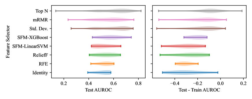
Figure 1: Distribution of feature selector performance by AUROC scores. Top N, Std. Dev. and mRMR include MI and STS scoring.

Scoring Performance

When evaluating the performance between the STS and MI scorers, as shown in Figure 2, we find that STS tends to perform better at selection than MI alone. When using a linear combination of both, we find the distribution of performance appears to be roughly the same as STS, but can achieve better test scores. For overfitting performance, we find a similar distribution of behavior. Scoring with STS tends to overfit much less than MI alone, and adding MI does not appear to change the distribution of performance as much.

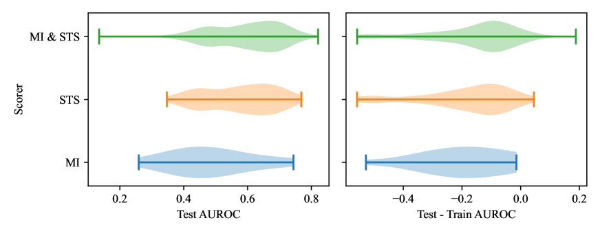
Figure 2: Performance of diferent feature scoring models by AUROC performance.

For scoring model, shown in Figure 4, we find that the differences between scoring model tend to be smaller. We do note that using a LLM appears to have a much narrower distribution of performance than the LMs tested, and the differences between choice of LLM appears to be smaller.

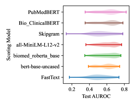
Figure 3: Distribution of STS scoring model performance by test AUROC

Finally, we find that the differences between a clinical and general fine-tuning dataset, shown in Figure 4, appear to negligible overall. This does not mean, however, that fine-tuning dataset has no overall effect. The best clinical/scientific pre-trained model, PubMedBERT, performed best with the combined fine-tuning dataset on MLP, which we believe is partially attributable to the difference between those scores and scores produced from the general dataset, as seen in Figures 5(c) and 5(b), respectively.

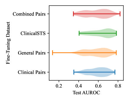
Figure 4: Distribution of STS fine-tuning dataset performance by test AUROC

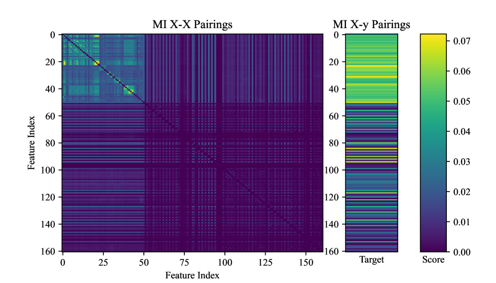
(a) MI scoring

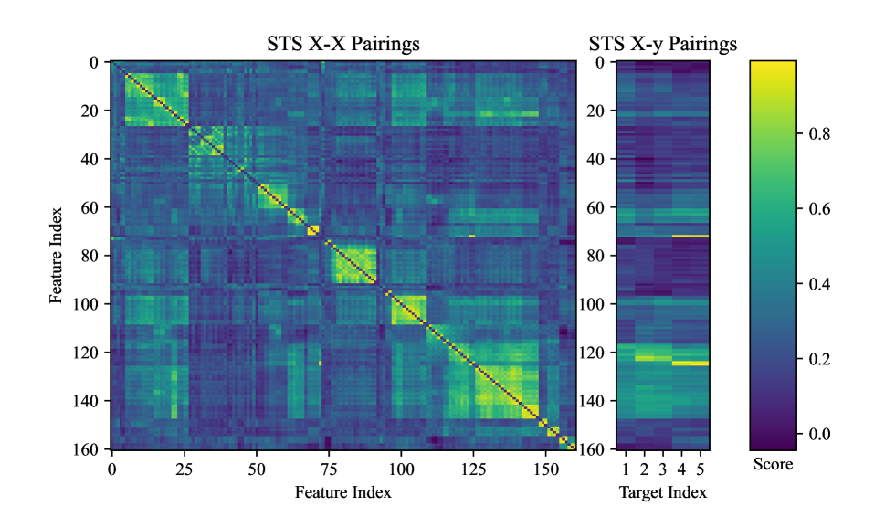
(b) STS scoring with PubMedBERT fine-tuned on the general vocab pairings.

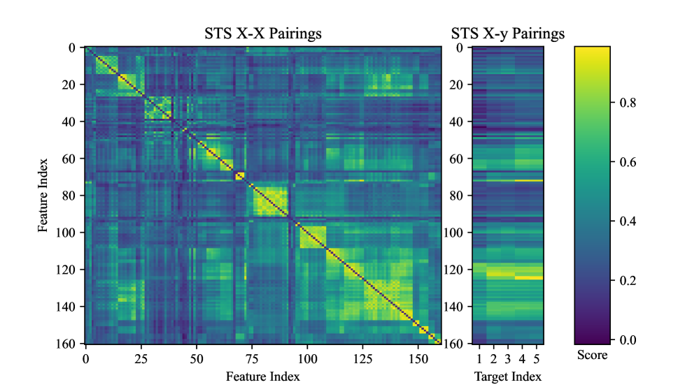
(c) STS scoring with PubMedBERT fine-tuned on the clinical vocab pairings.

Figure 5: Similarity pairings for different scoring models. Feature pairings are mirrored across the diagonal for viewability.

Selected Features

When evaluating the selected features, we see a noticeable difference between those selected using MI and STS scores. Figure 5, which shows MI and selected STS scores for the features and targets for the dataset, highlights why this difference exists, as the STS scores are capable of highlighting relationships between features and targets. The differences in the features selected, are shown in the supplemental material, as well as the performance of the model using the SHapley Additive exPlanations (SHAP) (Lundberg and Lee 2017) model when used with Gaussian Naïve Bayes.

Discussion

Feature Selection Performance

As shown in the previous section, using STS to select features appears to offer significant performance benefits over traditional feature selection methods.

One principal reason that the usage of STS appears to work better than statistical measures like MI is that STS scores are not affected by the curse of dimensionality. As can be seen with MI, many overlapping relationships can cause individual features to share little information, and features that we would expect to be more relevant than others will only have slightly more MI than those that would not be relevant. This is particularly evident when looking at mRMR scores calculated with MI scores, seen in the supplementary material, that dip into the negative: the subsequent feature learned is more redundant than it is relevant, yet there are many unselected features that we would consider to be truly relevant.

STS also provides a contrasting, non-correlated, source of information compared to statistical measures like MI. This fact can be seen from the strong contrast in highlighted regions between Figures 5(a) and 5(c)/5(b). When used in mRMR, STS is clearly more able to highlight redundant regions, especially along the diagonal, and is more able to distinguish between relevant and irrelevant features than MI. This is particularly useful for when MI that results from the training dataset fails to match what we might expect from the population sampled, as STS is not vulnerable to differences in the sample and population distributions.

Survey Writing & Feature Naming

The surveys used here were not designed in anticipation of this type of feature selection algorithm, but we anticipate survey designers may want to write questions with consideration to STS-based feature selection. We offer several guidelines for writing surveys or creating other forms of data with descriptive feature names.

Considerations should be made with respect to vocabulary. Words should primarily be derived from the vocabulary used to create tokens, and secondarily from the vocabulary used to fine-tune the pre-trained model to produce STS scores. Even if a ground-truth label is not given for a possible word-level STS pairing, the LM should be able to produce a meaningful STS score, as the LM will have learned word relationships in its vocabulary during pre-training. Acronyms should be expanded where possible, as an acronym may not be in either vocabulary, and thus be semantically meaningless.

Although the evidence presented here suggests that there may be a negligible difference between the performance of tokenizers—as the models tested use different tokenizers—subtle differences in tokenization may change the way that semantic relationships are captured. For example, Bostrom and Durrett (2020) note that byte-pair encoding (Gage 1994; Sennrich, Haddow, and Birch 2016) has weaker performance than unigram language modeling (Kudo 2018) with respect to morphological segmentations, implying that features tokenized with the latter algorithm may produce more meaningful STS scores.

Future Work

One area of future work is evaluating the performance of other measures, as the scorers evaluated here both have limitations. MI is incapable of measuring the true amount of information a feature contains in context with other features, and STS only represent semantic relationships without any regard to their underlying statistical relationship.

Future work could also consider the choice of other models for computing STS. We were not able to perform a complete evaluation due to resource limitations, and further analyses could evaluate larger models such as BioGPT (Luo et al. 2022) and GatorTron (Yang et al. 2022). The evidence presented here suggests that there may be marginal benefits to different scoring models.

Future work regarding STS-based feature selection could also consider the use of semantic pairs that specifically rate relevancy and redundancy between pairs of question embeddings, rather than similarity. Relevant and redundant questions may not always be semantically similar, and a dataset for fine-tuning upon this type of task may improve the performance of feature selection techniques that use STS.

Another potential area of future work would be to serialize the the feature selection task into a text prompt. Serialization of tablular data into a question prompt for a large language model can achieve high performance in a few-shot learning context (Hegselmann et al. 2022), and serialization of a feature selection objective may also be able to capture further semantic relationships between features.

Acknowledgements

This work was made possible through the support of the Department of Defense Congressionally Directed Medical Research Programs award W81XWH-21-1-0736. The authors would like to also thank Hanyang Liu for his valuable guidance on the final writing and publishing of this project.

References

- Abbas et al. (2018) Abbas, H.; Garberson, F.; Glover, E.; and Wall, D. P. 2018. Machine learning approach for early detection of autism by combining questionnaire and home video screening. Journal of the American Medical Informatics Association, 25(8): 1000–1007.
- Abut, Akay, and George (2016) Abut, F.; Akay, M. F.; and George, J. 2016. Developing new VO2max prediction models from maximal, submaximal and questionnaire variables using support vector machines combined with feature selection. Computers in biology and medicine, 79: 182–192.
- Alsentzer et al. (2019) Alsentzer, E.; Murphy, J. R.; Boag, W.; Weng, W.-H.; Jin, D.; Naumann, T.; and McDermott, M. 2019. Publicly available clinical BERT embeddings. arXiv preprint arXiv:1904.03323.
- Bostrom and Durrett (2020) Bostrom, K.; and Durrett, G. 2020. Byte pair encoding is suboptimal for language model pretraining. arXiv preprint arXiv:2004.03720.
- Cer et al. (2017) Cer, D.; Diab, M.; Agirre, E.; Lopez-Gazpio, I.; and Specia, L. 2017. SemEval-2017 Task 1: Semantic Textual Similarity Multilingual and Crosslingual Focused Evaluation. In Proceedings of the 11th International Workshop on Semantic Evaluation (SemEval-2017), 1–14. Vancouver, Canada: Association for Computational Linguistics.
- Chen and Guestrin (2016) Chen, T.; and Guestrin, C. 2016. Xgboost: A scalable tree boosting system. In Proceedings of the 22nd acm sigkdd international conference on knowledge discovery and data mining, 785–794.
- Chen, Wang, and Lu (2023) Chen, Y.; Wang, K.; and Lu, J. J. 2023. Feature selection for driving style and skill clustering using naturalistic driving data and driving behavior questionnaire. Accident Analysis & Prevention, 185: 107022.
- Chiu et al. (2018) Chiu, B.; Pyysalo, S.; Vulić, I.; and Korhonen, A. 2018. Bio-SimVerb and Bio-SimLex: Wide-coverage evaluation sets of word similarity in biomedicine. BMC Bioinformatics, 19.
- Devlin et al. (2018) Devlin, J.; Chang, M.-W.; Lee, K.; and Toutanova, K. 2018. Bert: Pre-training of deep bidirectional transformers for language understanding. arXiv preprint arXiv:1810.04805.
- Erhan et al. (2010) Erhan, D.; Courville, A.; Bengio, Y.; and Vincent, P. 2010. Why does unsupervised pre-training help deep learning? In Proceedings of the thirteenth international conference on artificial intelligence and statistics, 201–208. JMLR Workshop and Conference Proceedings.
- Gage (1994) Gage, P. 1994. A New Algorithm for Data Compression. C Users J., 12(2): 23–38.
- Gu et al. (2021) Gu, Y.; Tinn, R.; Cheng, H.; Lucas, M.; Usuyama, N.; Liu, X.; Naumann, T.; Gao, J.; and Poon, H. 2021. Domain-specific language model pretraining for biomedical natural language processing. ACM Transactions on Computing for Healthcare (HEALTH), 3(1): 1–23.
- Gururangan et al. (2020) Gururangan, S.; Marasović, A.; Swayamdipta, S.; Lo, K.; Beltagy, I.; Downey, D.; and Smith, N. A. 2020. Don’t Stop Pretraining: Adapt Language Models to Domains and Tasks. In Proceedings of ACL.
- Guyon et al. (2008) Guyon, I.; Gunn, S.; Nikravesh, M.; and Zadeh, L. A. 2008. Feature extraction: foundations and applications, volume 207. Springer.
- Haroutiunian et al. (2013) Haroutiunian, S.; Nikolajsen, L.; Finnerup, N. B.; and Jensen, T. S. 2013. The neuropathic component in persistent postsurgical pain: a systematic literature review. PAIN®, 154(1): 95–102.
- Hegselmann et al. (2022) Hegselmann, S.; Buendia, A.; Lang, H.; Agrawal, M.; Jiang, X.; and Sontag, D. 2022. TabLLM: Few-shot Classification of Tabular Data with Large Language Models. arXiv preprint arXiv:2210.10723.
- Joulin et al. (2016) Joulin, A.; Grave, E.; Bojanowski, P.; Douze, M.; Jégou, H.; and Mikolov, T. 2016. FastText.zip: Compressing text classification models. arXiv preprint arXiv:1612.03651.
- Kraskov, Stögbauer, and Grassberger (2004) Kraskov, A.; Stögbauer, H.; and Grassberger, P. 2004. Estimating mutual information. Physical review E, 69(6): 066138.
- Kudo (2018) Kudo, T. 2018. Subword Regularization: Improving Neural Network Translation Models with Multiple Subword Candidates. In Proceedings of the 56th Annual Meeting of the Association for Computational Linguistics (Volume 1: Long Papers), 66–75. Melbourne, Australia: Association for Computational Linguistics.
- Lampos, Zou, and Cox (2017) Lampos, V.; Zou, B.; and Cox, I. J. 2017. Enhancing feature selection using word embeddings: The case of flu surveillance. In Proceedings of the 26th International Conference on World Wide Web, 695–704.
- Lehman et al. (2023) Lehman, E.; Hernandez, E.; Mahajan, D.; Wulff, J.; Smith, M. J.; Ziegler, Z.; Nadler, D.; Szolovits, P.; Johnson, A.; and Alsentzer, E. 2023. Do We Still Need Clinical Language Models? arXiv preprint arXiv:2302.08091.
- Lundberg and Lee (2017) Lundberg, S. M.; and Lee, S.-I. 2017. A unified approach to interpreting model predictions. Advances in neural information processing systems, 30.
- Luo et al. (2022) Luo, R.; Sun, L.; Xia, Y.; Qin, T.; Zhang, S.; Poon, H.; and Liu, T.-Y. 2022. BioGPT: generative pre-trained transformer for biomedical text generation and mining. Briefings in Bioinformatics, 23(6).
- Manning (2022) Manning, C. D. 2022. Human language understanding & reasoning. Daedalus, 151(2): 127–138.
- May (2021) May, P. 2021. Machine translated multilingual STS benchmark dataset.
- Mikolov et al. (2013) Mikolov, T.; Chen, K.; Corrado, G.; and Dean, J. 2013. Efficient estimation of word representations in vector space. arXiv preprint arXiv:1301.3781.
- Mulyar, Schumacher, and Dredze (2019) Mulyar, A.; Schumacher, E.; and Dredze, M. 2019. semantic-text-similarity.
- Niemann et al. (2020) Niemann, U.; Brueggemann, P.; Boecking, B.; Mazurek, B.; and Spiliopoulou, M. 2020. Development and internal validation of a depression severity prediction model for tinnitus patients based on questionnaire responses and socio-demographics. Scientific reports, 10(1): 4664.
- Oniani, Sivarajkumar, and Wang (2022) Oniani, D.; Sivarajkumar, S.; and Wang, Y. 2022. Few-Shot Learning for Clinical Natural Language Processing Using Siamese Neural Networks. arXiv preprint arXiv:2208.14923.
- Pedersen et al. (2007) Pedersen, T.; Pakhomov, S. V.; Patwardhan, S.; and Chute, C. G. 2007. Measures of semantic similarity and relatedness in the biomedical domain. Journal of biomedical informatics, 40(3): 288–299.
- Pedregosa et al. (2011) Pedregosa, F.; Varoquaux, G.; Gramfort, A.; Michel, V.; Thirion, B.; Grisel, O.; Blondel, M.; Prettenhofer, P.; Weiss, R.; Dubourg, V.; et al. 2011. Scikit-learn: Machine learning in Python. the Journal of machine Learning research, 12: 2825–2830.
- Peng, Long, and Ding (2005) Peng, H.; Long, F.; and Ding, C. 2005. Feature selection based on mutual information criteria of max-dependency, max-relevance, and min-redundancy. IEEE Transactions on pattern analysis and machine intelligence, 27(8): 1226–1238.
- Radford et al. (2019) Radford, A.; Wu, J.; Child, R.; Luan, D.; Amodei, D.; Sutskever, I.; et al. 2019. Language models are unsupervised multitask learners. OpenAI blog, 1(8): 9.
- Ramírez-Gallego et al. (2017) Ramírez-Gallego, S.; Lastra, I.; Martínez-Rego, D.; Bolón-Canedo, V.; Benítez, J. M.; Herrera, F.; and Alonso-Betanzos, A. 2017. Fast-mRMR: Fast minimum redundancy maximum relevance algorithm for high-dimensional big data. International Journal of Intelligent Systems, 32(2): 134–152.
- Řehůřek and Sojka (2010) Řehůřek, R.; and Sojka, P. 2010. Software Framework for Topic Modelling with Large Corpora. In Proceedings of the LREC 2010 Workshop on New Challenges for NLP Frameworks, 45–50. Valletta, Malta: ELRA. http://is.muni.cz/publication/884893/en.
- Reimers and Gurevych (2019) Reimers, N.; and Gurevych, I. 2019. Sentence-bert: Sentence embeddings using siamese bert-networks. arXiv preprint arXiv:1908.10084.
- Remeseiro and Bolon-Canedo (2019) Remeseiro, B.; and Bolon-Canedo, V. 2019. A review of feature selection methods in medical applications. Computers in biology and medicine, 112: 103375.
- Ross (2014) Ross, B. C. 2014. Mutual information between discrete and continuous data sets. PloS one, 9(2): e87357.
- Roy and Pan (2021) Roy, A.; and Pan, S. 2021. Incorporating medical knowledge in BERT for clinical relation extraction. In Proceedings of the 2021 conference on empirical methods in natural language processing, 5357–5366.
- Saridewi and Sari (2020) Saridewi, V. S.; and Sari, R. F. 2020. Feature selection in the human aspect of information security questionnaires using multicluster feature selection. International Journal of Advanced Science and Technology, 29(7 Special Issue): 3484–3493.
- Sennrich, Haddow, and Birch (2016) Sennrich, R.; Haddow, B.; and Birch, A. 2016. Neural Machine Translation of Rare Words with Subword Units. In Proceedings of the 54th Annual Meeting of the Association for Computational Linguistics (Volume 1: Long Papers), 1715–1725. Berlin, Germany: Association for Computational Linguistics.
- Singhal et al. (2022) Singhal, K.; Azizi, S.; Tu, T.; Mahdavi, S. S.; Wei, J.; Chung, H. W.; Scales, N.; Tanwani, A.; Cole-Lewis, H.; Pfohl, S.; et al. 2022. Large Language Models Encode Clinical Knowledge. arXiv preprint arXiv:2212.13138.
- Urbanowicz et al. (2018) Urbanowicz, R. J.; Olson, R. S.; Schmitt, P.; Meeker, M.; and Moore, J. H. 2018. Benchmarking relief-based feature selection methods for bioinformatics data mining. Journal of biomedical informatics, 85: 168–188.
- Vila et al. (2020) Vila, M. R.; Todorovic, M. S.; Tang, C.; Fisher, M.; Steinberg, A.; Field, B.; Bottros, M. M.; Avidan, M. S.; and Haroutounian, S. 2020. Cognitive flexibility and persistent post-surgical pain: the FLEXCAPP prospective observational study. British journal of anaesthesia, 124(5): 614–622.
- Wainer and Cawley (2021) Wainer, J.; and Cawley, G. 2021. Nested cross-validation when selecting classifiers is overzealous for most practical applications. Expert Systems with Applications, 182: 115222.
- Wang et al. (2020) Wang, Y.; Afzal, N.; Fu, S.; Wang, L.; Shen, F.; Rastegar-Mojarad, M.; and Liu, H. 2020. MedSTS: a resource for clinical semantic textual similarity. Language Resources and Evaluation, 54: 57–72.
- Washington et al. (2019) Washington, P.; Paskov, K. M.; Kalantarian, H.; Stockham, N.; Voss, C.; Kline, A.; Patnaik, R.; Chrisman, B.; Varma, M.; Tariq, Q.; et al. 2019. Feature selection and dimension reduction of social autism data. In Pacific Symposium on Biocomputing 2020, 707–718.
- Wei et al. (2023) Wei, C.; Wang, Y.-C.; Wang, B.; and Kuo, C.-C. J. 2023. An Overview on Language Models: Recent Developments and Outlook. arXiv preprint arXiv:2303.05759.
- Wolf et al. (2019) Wolf, T.; Debut, L.; Sanh, V.; Chaumond, J.; Delangue, C.; Moi, A.; Cistac, P.; Rault, T.; Louf, R.; Funtowicz, M.; et al. 2019. Huggingface’s transformers: State-of-the-art natural language processing. arXiv preprint arXiv:1910.03771.
- Wornow et al. (2023) Wornow, M.; Xu, Y.; Thapa, R.; Patel, B.; Steinberg, E.; Fleming, S.; Pfeffer, M. A.; Fries, J.; and Shah, N. H. 2023. The shaky foundations of large language models and foundation models for electronic health records. npj Digital Medicine, 6(1): 135.
- Xiong et al. (2020) Xiong, Y.; Chen, S.; Chen, Q.; Yan, J.; Tang, B.; et al. 2020. Using character-level and entity-level representations to enhance bidirectional encoder representation from transformers-based clinical semantic textual similarity model: ClinicalSTS modeling study. JMIR Medical Informatics, 8(12): e23357.
- Yang et al. (2022) Yang, X.; Chen, A.; PourNejatian, N.; Shin, H. C.; Smith, K. E.; Parisien, C.; Compas, C.; Martin, C.; Costa, A. B.; Flores, M. G.; et al. 2022. A large language model for electronic health records. npj Digital Medicine, 5(1): 194.