On Estimating the Gradient of the Expected Information Gain in Bayesian Experimental Design

Abstract

Bayesian Experimental Design (BED), which aims to find the optimal experimental conditions for Bayesian inference, is usually posed as to optimize the expected information gain (EIG). The gradient information is often needed for efficient EIG optimization, and as a result the ability to estimate the gradient of EIG is essential for BED problems. The primary goal of this work is to develop methods for estimating the gradient of EIG, which, combined with the stochastic gradient descent algorithms, result in efficient optimization of EIG. Specifically, we first introduce a posterior expected representation of the EIG gradient with respect to the design variables. Based on this, we propose two methods for estimating the EIG gradient, UEEG-MCMC that leverages posterior samples generated through Markov Chain Monte Carlo (MCMC) to estimate the EIG gradient, and BEEG-AP that focuses on achieving high simulation efficiency by repeatedly using parameter samples. Theoretical analysis and numerical studies illustrate that UEEG-MCMC is robust agains the actual EIG value, while BEEG-AP is more efficient when the EIG value to be optimized is small. Moreover, both methods show superior performance compared to several popular benchmarks in our numerical experiments.

Introduction

The advancement of science and engineering heavily relies on the acquisition of data through experiments. However, conducting experiments can be resource-intensive and time-consuming. To maximize the information gained from collected data and optimize experimental outcomes, researchers turn to Bayesian experimental design (BED) which offers a systematic and powerful framework for making informed decisions about experimental setups and selecting optimal conditions for data collection. At its core, BED aims to strategically allocate resources to collect the most informative data, which leads to more accurate parameter estimation, model validation, and decision-making. It has been broadly applied in diverse scientific fields, including pharmacokinetic study (Ryan et al. 2014), drug discovery (Lyu et al. 2019), systems biology (Kreutz and Timmer 2009), compressed sensing (Seeger and Nickisch 2008) and physics simulations (Melendez et al. 2021).

Mathematically, BED can be formulated as an optimization problem, where the objective is to maximize a specific function known as the utility function. The choice of the utility function is often driven by the purpose of the BED. In this paper, our focus lies on BED’s application to precise parameter estimation. Various utility functions have been employed to address parameter estimation challenges, and some notable examples include Bayesian A-posterior precision, Bayesian D-posterior precision, quadratic loss and expected information gain (EIG) (see (Ryan et al. 2016) for a review). While the EIG stands out for its exceptional theoretical appeal among these functions, its use has been a long-standing challenge historically due to the computational complexity associated with estimating the evidence or marginal likelihood, which is analytically intractable or computationally expensive to evaluate directly. Consequently, BED based on EIG was once restricted to special cases where analytical solutions or simplifying assumptions allowed for a tractable computation of the evidence (Borth 1975; Lewi, Butera, and Paninski 2009). Fortunately, recent advancements in Artificial Intelligence (AI) tools, particularly in neural EIG estimators and automatic differentiation frameworks, have significantly alleviated the computational challenge, enabling the efficient implementation of EIG-based BED in a wide range of non-linear and high-dimensional problems.

Accurate estimation of EIG has been widely recognized as one of the most significant barriers of EIG-based BED. However, our primary interest is not in the exact value of the EIG, but rather in the design variables that maximize the value. Motivated by this viewpoint, an alternative strategy is directly estimating the gradient of EIG w.r.t. the design variables and then using stochastic gradient descent to search for the optimal design. In this paper, we propose two methods for estimating the EIG gradient. The first method, UEEG-MCMC, applies posterior samples generated by Markov Chain Monte Carlo (MCMC) to estimate the EIG gradient. It is shown effective across different scenarios, regardless of the ground-truth EIG values. The second method, BEEG-AP, is more simulation-efficient. However, its performance suffers when dealing with problems that have large ground-truth EIG values. The paper establishes a connection with nested Monte Carlo to analyze this behavior, shedding light on the limitations of BEEG-AP in such cases.

We validate the aforementioned attributes of the two proposed methods through a meticulous numerical experiment and diverse applications featuring varying expected EIG levels. Additionally, comprehensive comparisons are made with several bench-marking approaches, revealing the superior performance of our proposed methods.

Related Work

Rainforth et al.(Rainforth et al. 2023) provide a thorough review of modern methods for Bayesian experimental design. Early schemes for Bayesian experimental design used separate stages to estimate the Expected Information Gain (EIG) and optimize the design variables $\lambda$, both of which can be challenging tasks. For EIG estimation, the main computational challenge arises from the intractability of $p(y|\lambda)$ and several methods have been proposed to solve this problem. Notably, Nested Monte Carlo (NMC) (Rainforth et al. 2018; Ryan 2003) emerged as a prominent method in this area. Additionally, Variational EIG estimators (also known as variational mutual information estimators) (Foster et al. 2019; Barber and Agakov 2004; Donsker and Varadhan 1975; Nguyen, Wainwright, and Jordan 2010) combined with deep learning techniques (Belghazi et al. 2018; Oord, Li, and Vinyals 2018; Alemi et al. 2016; Song and Ermon 2019) showed significant progress. Furthermore, alternative approaches for EIG estimation included using ratio estimation (Thomas et al. 2022) as proposed in (Kleinegesse and Gutmann 2019), and bounding EIG from below by two or more entropies in the data space (Ao and Li 2020) which are then be estimated by entropy estimation methods (Kraskov, Stögbauer, and Grassberger 2004). A direct lower bound estimation for EIG was introduced in (Tsilifis, Ghanem, and Hajali 2017) for models with fixed normally distributed measurement noises, and the EIG Laplace approximation was proposed in (Long et al. 2013). Regarding the optimization of $\lambda$, conventional gradient-free approaches such as Bayesian optimization (BO) (Snoek, Larochelle, and Adams 2012), Simultaneous perturbation stochastic approximation (SPSA) (Spall 1998), simulation-based optimization (SBO)(Müller 2005), and Nelder-Mead nonlinear simplex (NMNS)(Nelder and Mead 1965) were commonly employed. However, these methods encountered scalability issues when dealing with high-dimensional design variable spaces.

Recent advancements have introduced efficient gradient-based approaches that leverage the reparameterization trick and automatic differentiation frameworks. These methods, such as those proposed in (Foster et al. 2020; Kleinegesse and Gutmann 2020; Zhang, Bi, and Zhang 2021; Zaballa and Hui 2023), allow for simultaneous optimization of both the variational parameters and the design variables. Moreover, Goda et al. (Goda et al. 2022) presented a method that directly obtains an unbiased estimator of the EIG gradient using a randomized version of multilevel Monte Carlo (MLMC) method (Rhee and Glynn 2015). Furthermore, gradient estimators for implicit models (Li and Turner 2017; Wen et al. 2021; Lim et al. 2020; Shi, Sun, and Zhu 2018) with score matching techniques (Hyvärinen and Dayan 2005; Song et al. 2020) have emerged as another avenue for optimizing $\lambda$ in a gradient-based way. Despite receiving limited attention in the Bayesian experimental design community, these methods hold promise and deserve further exploration.

Preliminary Knowledge

Problem Formulation

This section defines the variables and functions involved as well as the primary objective of Bayesian experimental design. Let $\lambda\in\mathcal{D}$ be the design variables that can be controlled by users. The parameters to be inferred from the observed data $y$ are denoted by $\theta$ and $\pi_{\mathrm{\theta}}(\theta)$ denotes its prior that represents our knowledge or belief about the parameters before observing any data. $\epsilon$ represents the base model noises generated from a known distribution $\pi_{\mathrm{\epsilon}}(\epsilon)$. The process of simulating the observed data can be modeled by a sampling path

$$y=g(\theta,\epsilon,\lambda).$$ (1)

In this context, we assume the existence of a tractable likelihood function $l(y|\theta,\lambda)$, which is derived from the sampling path. However, it is important to note that the marginal likelihood $p(y|\lambda)$ is not available in closed-form. Under certain design $\lambda$, the expected information gain (EIG) is defined as

$$U(\lambda)=\mathbb{E}_{\pi_{\mathrm{\theta}(\theta)l(y|\theta,\lambda)}}[\log l(y|\theta,\lambda)]-\mathbb{E}_{p(y|\lambda)}[\log p(y|\lambda)].$$ (2)

It represents the expected amount of information that observations $y$ provide about $\theta$ and is well known as the mutual information (Cover 1999) between $\theta$ and $y$ in information theory community. The objective of Bayesian experimental design is then to maximize the EIG over the design variable space $\mathcal{D}$

$$\lambda^{*}=\underset{\lambda\in\mathcal{D}}{\arg\max}~{}U(\lambda).$$ (3)

Simulation Cost

Estimating and optimizing the EIG entails generating observation samples and evaluating the corresponding likelihood values. This process can be computationally demanding, and its efficiency is of paramount importance in practical applications. In this section, we will illustrate how to quantify the simulation cost during the process when explicit models are considered. For explicit models, the sampling path can typically be written as a hierarchical structure

$$y=g(f(\theta,\lambda),\epsilon,\theta,\lambda),$$ (4)

where $f$ is the forward model which dominates the main computational cost. Examples of the commonly used hierarchical structure include:

$$\mathrm{Additive~{}noise:~{}}y=f(\theta,\lambda)+\sigma(\theta,\lambda)\epsilon.$$ (5)

$$\mathrm{Multiplicative~{}noise:~{}}y=f(\theta,\lambda)(1+\sigma(\theta,\lambda)\epsilon).$$ (6)

$$\mathrm{Mixture~{}of~{}noises:~{}}y\!=\!f(\theta\!,\lambda)(1+\sigma_{1}(\theta\!,\lambda)\epsilon_{1})+\sigma_{2}(\theta\!,\lambda)\epsilon_{2}.$$ (7)

For simplicity, we take the case of additive noise for example to analyze the simulation cost concerned in applications. Given a fixed parameter $\theta^{*}$, simulating multiple observations (e.g. $y^{(k)}=f(\theta^{*},\lambda)+\sigma(\theta^{*},\lambda)\epsilon^{(k)}$, $k=1,...,K$) only involves a single simulation (i.e. $f(\theta^{*},\lambda)$) of the forward model. Likewise, since the likelihood function can be analytically written as

$$l(y|\theta,\lambda)=\pi_{\mathrm{\epsilon}}\Big{(}\frac{y-f(\theta,\lambda)}{\sigma(\theta,\lambda)}\Big{)},$$ (8)

evaluating the values of the likelihood w.r.t. multiple observations (e.g. $l(y^{(k)}|\theta^{*},\lambda)$, $k=1,...,K$) also requires only a single forward pass of $f$. Thus, the simulation cost of generating observations from and evaluating the likelihood is directly related to the number of different parameters involved. This observation is important for the analysis of simulation costs of estimators in the later sections.

Posterior Expected Representations of the EIG Gradient

In this section, we introduce a novel representation of the EIG gradient that offers new insights into the development of efficient gradient estimators. To start with, we analyze the difficulty in directly computing the EIG gradient w.r.t. the design variables $\lambda$. Estimating the gradient of Eq. (2) directly with score-function estimators (Mohamed et al. 2020) could lead to high variance. As a result, practitioners often turn to pathwise gradient estimators (also known as the reparameterization tricks) (Mohamed et al. 2020), as an alternative strategy for estimating this gradient:

$$\nabla_{\lambda}U(\lambda)= \nabla_{\lambda}\mathbb{E}_{\pi_{\mathrm{\theta}(\theta)\pi_{\epsilon}(\epsilon)}}[\log l(g(\theta,\epsilon,\lambda)|\theta,\lambda)]$$ (9)

$$\quad\quad\quad\quad-\nabla_{\lambda}\mathbb{E}_{\pi_{\mathrm{\theta}(\theta)\pi_{\epsilon}(\epsilon)}}[\log p(g(\theta,\epsilon,\lambda)|\lambda)]$$

$$= \mathbb{E}_{\pi_{\mathrm{\theta}(\theta)\pi_{\epsilon}(\epsilon)}}[\nabla_{\lambda}\log l(g(\theta,\epsilon,\lambda)|\theta,\lambda)]$$

$$\quad\quad\quad\quad-\mathbb{E}_{\pi_{\mathrm{\theta}(\theta)\pi_{\epsilon}(\epsilon)}}[\nabla_{\lambda}\log p(g(\theta,\epsilon,\lambda)|\lambda)].$$

While obtaining $\nabla_{\lambda}g(\theta,\epsilon,\lambda)$ is typically straightforward using modern automatic differentiation frameworks (e.g. Tensorflow (Abadi 2016) and Pytorch (Paszke et al. 2017)), the score function $\nabla_{y}\log p(y|\lambda)$ usually does not have an analytical form, rendering the second term of the above estimator intractable. To address this challenge, we apply the key idea in (Brehmer et al. 2020), which involves using the tractable score of likelihood $\nabla_{y}\log l(y|\theta,\lambda)$ to estimate the intractable score function $\nabla_{y}\log p(y|\lambda)$. This can be summarized as the following Lemma 1.

Lemma 1.

The gradient of the logarithm of the marginal density w.r.t. the experimental condition $\lambda$ admits the following representation:

$$\nabla_{\lambda}\log p(g(\theta,\epsilon,\lambda))|\lambda)$$ (10)

$$\quad\quad\quad\quad=-\mathbb{E}_{q(\theta^{\prime}|g(\theta,\epsilon,\lambda),\lambda)}[\nabla_{\lambda}\log l(g(\theta,\epsilon,\lambda)|\theta^{\prime},\lambda)],$$

where $q(\theta^{\prime}|y,\lambda)\propto\pi_{\mathrm{\theta}}(\theta^{\prime})l(y|\theta^{\prime},\lambda)$ is the posterior density of parameters given the observation sample $y$.

Using this lemma, we derive an entropy gradient estimator for the marginal distribution of $y$ as stated in Theorem 1.

Theorem 1.

The gradient of the entropy $H(p(y|\lambda))$ w.r.t. the experimental condition $\lambda$ satisfies

$$\nabla_{\lambda}H(p(y|\lambda))$$ (11)

$$= -\mathbb{E}_{\pi_{\mathrm{\theta}}(\theta)\pi_{\mathrm{\epsilon}}(\epsilon)q(\theta^{\prime}|g(\theta,\epsilon,\lambda),\lambda)}[\nabla_{\lambda}\log l(g(\theta,\epsilon,\lambda)|\theta^{\prime},\lambda)],$$

where $q(\theta^{\prime}|y,\lambda)\propto\pi_{\mathrm{\theta}}(\theta^{\prime})l(y|\theta^{\prime},\lambda)$ is the posterior density of parameters given the observation sample $y$.

Using Theorem 1, we can get a posterior expected representation of the EIG gradient, as stated in the following Corollary 1.

Corollary 1.

The gradient of the EIG $U(\lambda)$ w.r.t. the experimental condition $\lambda$ satisfies

$$\nabla_{\lambda}U(\lambda)$$ (12)

$$\quad=\mathbb{E}_{\pi_{\mathrm{\theta}}(\theta)\pi_{\mathrm{\epsilon}}(\epsilon)q(\theta^{\prime}|g(\theta,\epsilon,\lambda),\lambda)}[\nabla_{\lambda}\log l(g(\theta,\epsilon,\lambda)|\theta,\lambda)$$

$$\quad\quad\quad\quad\quad\quad\quad\quad\quad\quad\quad\quad-\nabla_{\lambda}\log l(g(\theta,\epsilon,\lambda)|\theta^{\prime},\lambda)],$$

where $q(\theta^{\prime}|y,\lambda)\propto\pi_{\mathrm{\theta}}(\theta^{\prime})l(y|\theta^{\prime},\lambda)$ is the posterior density of parameters given the observation sample $y$.

Estimating the EIG Gradient

Building upon the posterior expected representation of the EIG gradient in Eq. (12), we propose two estimators of EIG gradient. When integrated with stochastic gradient descent algorithms, these estimators seamlessly evolve into the respective algorithms for Bayesian experimental design. For simplicity, we denote the observation samples generated from the sampling path as $y^{(i)}(\lambda)=g(\theta^{(i)},\epsilon^{(i)},\lambda)$ throughout this section.

Unbiased Estimation of EIG Gradient with Markov Chain Monte Carlo

The most straightforward method to estimate the expectation in Eq. (12) is utilizing MCMC schemes. Specifically, giving samples $\{\theta^{(i)}\}_{i=1}^{M}$ and $\{\epsilon^{(i)}\}_{i=1}^{M}$ drawn from $\pi_{\mathrm{\theta}}(\theta)\pi_{\mathrm{\epsilon}}(\epsilon)$, the expectation in Eq. (12) can be estimated by Monte Carlo average as

$$\nabla_{\lambda}U(\lambda) \approx\frac{1}{M}\sum_{i=1}^{M}\nabla_{\lambda}\log l(y^{(i)}(\lambda)|\theta^{(i)},\lambda)$$ (13)

$$-\frac{1}{M}\sum_{i=1}^{M}\mathbb{E}_{q(\theta^{\prime}|y^{(i)}(\lambda),\lambda)}[\nabla_{\lambda}\log l(y^{(i)}(\lambda)|\theta^{\prime},\lambda)].$$

Ideally if we can draw samples $\{\theta^{(i,j)}\}_{j=1}^{N}$ exactly from the posterior $q(\theta^{\prime}|y^{(i)}(\lambda),\lambda)$, we can obtain an unbiased estimator of $\mathbb{E}_{q(\theta^{\prime}|y^{(i)}(\lambda),\lambda)}[\nabla_{\lambda}\log l(y^{(i)}(\lambda)|\theta^{\prime},\lambda)]$:

$$\mathbb{E}_{q(\theta^{\prime}|y^{(i)}(\lambda),\lambda)}[\nabla_{\lambda}\log l(y^{(i)}(\lambda)|\theta^{\prime},\lambda)]$$ (14)

$$\quad\quad\quad\quad\quad\quad\quad\quad\approx\frac{1}{N}\sum_{j=1}^{N}\nabla_{\lambda}\log l(y^{(i)}(\lambda)|\theta^{(i,j)},\lambda).$$

Combining Eq. (13) and Eq. (14) yields an unbiased estimator of EIG gradient in theory. In reality however, one often relies on Markov Chain Monte Carlo (MCMC) methods to sample the posterior distribution, which draws biased samples from the posterior distribution. We refer to the method as unbiased estimation of EIG gradient with MCMC (UEEG-MCMC). The simulation cost of a single gradient estimation for UEEG-MCMC is $O(M\times L)$, where $L$ is the number of simulations used to perform MCMC. We reinstate that a finite-length MCMC can not produce unbiased samples from the posterior and as such it causes bias in the gradient estimator. Nevertheless, we emphasize that the bias lies in the samples and the estimator itself is unbiased provided that samples are generated perfectly from the posterior. As will be shown in the numerical examples, the bias due to MCMC is often much smaller than those in other methods especially for problems with large EIG values. Moreover, while we adopt MCMC for sampling the posterior here, the proposed method can be implemented with any sampling methods. To this end, if more effective sampling methods are available, they can be used instead of MCMC to reduce the estimation bias.

Biased Estimation of EIG Gradient with Atomic Priors

Generating an observation from or evaluating the likelihood for each new parameter sample requires to simulate the physical model considered once more. For expensive physical models, this constitutes the most significant computational cost.

In this section, we show how to obtain a simulation-efficient approach using atomic priors. Suppose a finite set of parameter-noise pairs $\Omega=\{(\theta^{(i)},\epsilon^{(i)})\}_{i=1}^{M}$ are generated, where $(\theta^{(i)},\epsilon^{(i)})\sim\pi_{\mathrm{\theta}}(\theta)\pi_{\mathrm{\epsilon}}(\epsilon)$, and we denote $\Theta=\{\theta^{(i)}\}_{i=1}^{M}$. Replacing the sampling distributions $\pi_{\mathrm{\theta}}(\theta)\pi_{\mathrm{\epsilon}}(\epsilon)$ by $U_{\Omega}$ and $\pi_{\mathrm{\theta}}(\theta^{\prime})$ by $U_{\Theta}$, where $U$ denotes the uniform distribution on the given set, we can approximate the sampling distribution over which the expected value is taken in Eq. (12) as

$$\pi_{\mathrm{\theta}}(\theta)\pi_{\mathrm{\epsilon}}(\epsilon)q(\theta^{\prime}|g(\theta,\epsilon,\lambda),\lambda)$$ (15)

$$= \frac{\pi_{\mathrm{\theta}}(\theta)\pi_{\mathrm{\epsilon}}(\epsilon)\pi_{\mathrm{\theta}}(\theta^{\prime})l(g(\theta,\epsilon,\lambda)|\theta^{\prime},\lambda)}{\int\pi_{\mathrm{\theta}}(\theta^{\prime})l(g(\theta,\epsilon,\lambda)|\theta^{\prime},\lambda)d\theta^{\prime}}$$

$$\approx \sum_{i=1}^{M}\frac{\sum_{j=1}^{M}\delta_{\theta^{(i)}}(\theta)\delta_{\epsilon^{(i)}}(\epsilon)\delta_{\theta^{(j)}}(\theta^{\prime})l(y^{(i)}(\lambda)|\theta^{(j)},\lambda)}{\sum_{j=1}^{M}l(y^{(i)}(\lambda)|\theta^{(j)},\lambda)}.$$

Given this approximation of sampling distribution, we finally obtain a biased estimator of EIG gradient

$$\nabla_{\lambda}U(\lambda)$$ (16)

$$\approx \sum_{i=1}^{M}\frac{\sum_{j=1}^{M}l(y^{(i)}(\lambda)|\theta^{(j)},\lambda)\nabla_{\lambda}\log\big{[}\frac{l(y^{(i)}(\lambda)|\theta^{(i)},\lambda)}{l(y^{(i)}(\lambda)|\theta^{(j)},\lambda)}\big{]}}{\sum_{j=1}^{M}l(y^{(i)}(\lambda)|\theta^{(j)},\lambda)}.$$

we refer to it as biased estimation of EIG gradient with atomic priors (BEEG-AP). As it requires only one batch of parameter samples for each gradient estimation, the simulation cost amounts to $O(M)$.

Unifying BEEG-AP and NMC

To provide a more comprehensive understanding of BEEG-AP, this section reveals its close connection to NMC. Indeed, BEEG-AP can be regarded as an approach that directly computes the gradient of the NMC estimator with sample reuse technique (srNMC) in (Huan and Marzouk 2013). We start this section by revisiting the concepts of NMC and srNMC.

The naïve NMC estimates the EIG as

$$U(\lambda)\approx\frac{1}{M}\sum_{i=1}^{M}\log\frac{l(y^{(i)}(\lambda)|\theta^{(i)},\lambda)}{\frac{1}{N}\sum_{j=1}^{N}l(y^{(i)}(\lambda)|\theta^{(i,j)},\lambda)},$$ (17)

where $\theta^{(i)}\sim\pi_{\mathrm{\theta}}(\theta)$, $\epsilon^{(i)}\sim\pi_{\mathrm{\epsilon}}(\epsilon)$ and $\theta^{(i,j)}\sim\pi_{\mathrm{\theta}}(\theta)$. This approximation requires a simulation cost of $O(M\times N)$. To reduce the cost to $O(M)$, Huan & Marzouk (Huan and Marzouk 2013) propose reusing the batch of prior samples for the outer Monte Carlo sum in all inner Monte Carlo estimations (i.e., $\theta^{(i,j)}=\theta^{(j)}$ and $N=M$). This yields a more simulation-efficient estimator of EIG

$$\widehat{U}_{srNMC}^{M}(\lambda)=\frac{1}{M}\sum_{i=1}^{M}\log\frac{l(y^{(i)}(\lambda)|\theta^{(i)},\lambda)}{\frac{1}{M}\sum_{j=1}^{M}l(y^{(i)}(\lambda)|\theta^{(j)},\lambda)}.$$ (18)

This estimator is also related to the InfoNCE with a tractable conditional (Oord, Li, and Vinyals 2018; Poole et al. 2019), often utilized for the mutual information estimation in representation learning. In addition, similar sample reuse techniques have been applied to portfolio risk measurement problems (Zhang et al. 2022; Feng and Li 2022).

Now it is evident that the BEEG-AP can be directly derived from the gradient of Eq. (18) w.r.t. $\lambda$. This observation allows us to explore the theoretical behavior of the BED with BEEG-AP by investigating the convergence properties of the srNMC. The original paper of (Huan and Marzouk 2013) only provides a simple numerical study of the bias of srNMC. Here, we give a more rigorous convergence analysis as the following theorems.

Theorem 2.

The expectation of $\widehat{U}_{srNMC}^{M}(\lambda)$ satisfies the following:

1. $\mathbb{E}[\widehat{U}_{srNMC}^{M}(\lambda)]$ is a lower bound on $U(\lambda)$ for any $M>0$.

2. $\mathbb{E}[\widehat{U}_{srNMC}^{M}(\lambda)]$ is monotonically increasing in $M$, i.e., $\mathbb{E}[\widehat{U}_{srNMC}^{M_{1}}(\lambda)]\leq\mathbb{E}[\widehat{U}_{srNMC}^{M_{2}}(\lambda)]$ for $0\leq M_{1}\leq M_{2}$.

Theorem 3.

If $l(g(\theta,\epsilon,\lambda)|\theta^{\prime},\lambda)$ is bounded away from 0 and uniformly bounded from above (i.e., $C_{1}\leq l(g(\theta,\epsilon,\lambda)|\theta^{\prime},\lambda)\leq C_{2}$ a.s. for some positive constants $C_{1}$ and $C_{2}$), then the mean squared error of $\widehat{U}_{srNMC}^{M}(\lambda)$ converges to 0 at rate $O(1/M)$.

Theorem 2 indicates that the srNMC provides a lower bound estimation for the EIG and the gap can be increasingly narrowed as $M$ increases. This suggests that BED with BEEG-AP aims to use stochastic gradients to maximize a lower bound of the ground-truth EIG. Theorem 3 further establishes the consistency of srNMC and obtains a linear convergence rate of $O(1/M)$ under certain assumptions, indicating that the optimization objective of BED with BEEG-AP can be sufficiently close to true EIG as we increase the number of samples $M$. However, the following Theorem 4 suggests that achieving a neglected error is challenging in practice when the ground-truth EIG is large, even when these assumptions are admitted.

Theorem 4.

For any $C$ satisfying $0\leq C\leq U(\lambda)/2$, if $M\leq\exp(U(\lambda)/2)$, we have

$$U(\lambda)-\widehat{U}_{srNMC}^{M}(\lambda)>C.$$ (19)

Indeed, this theorem tells us that the simulation cost required grows exponentially with the ground-truth EIG to achieve a reasonable error bound.

Experiments

A large variety of BED methods could exhibit poor performance due to the presence of large EIG values in the experiments to be designed. Before diving into numerical demonstrations (see https://github.com/ziq-ao/GradEIG for the research code and Appendix for further details of our experiments), we list a few bench-marking approaches and briefly discuss the above limitation they have in common.

PCE. Prior contrastive estimation (PCE) (Foster et al. 2020) estimates the EIG as

$$\widehat{U}_{PCE}^{M,N}(\lambda)=\frac{1}{M}\sum_{i=1}^{M}\log\frac{l(y^{(i)}(\lambda)|\theta^{(i)},\lambda)}{\frac{1}{N+1}\sum_{j=0}^{N}l(y^{(i)}(\lambda)|\theta^{(i,j)},\lambda)},$$ (20)

where $\theta^{(i)},\epsilon^{(i)}\sim\pi_{\theta}(\theta)\pi_{\epsilon}(\epsilon)$, $\theta^{(i,0)}=\theta^{(i)}$ and $\theta^{(i,j)}\sim\pi_{\theta}(\theta)$ for $j=1,...,N$. In contrast to srNMC, PCE only reuses one outer Monte Carlo sample in each inner Monte Carlo estimation, resulting in a simulation cost of $O(M\times N)$. It is easy to check that $\widehat{U}_{PCE}^{M,N}(\lambda)$ does not exceed $\log N$, so PCE shares a similar result to the one stated in Theorem 4, implying its simulation inefficiency for estimating large EIG values.

ACE. To improve the inner Monte Carlo in the denominator, adaptive contrastive estimation (ACE) (Foster et al. 2020) introduces a posterior inference network $q_{\phi}$ parameterized by $\phi$ and use it as the proposal distribution for sampling, i.e.,

$$\widehat{U}_{ACE}^{M,N}(\lambda)$$ (21)

$$\quad=\frac{1}{M}\sum_{i=1}^{M}\log\frac{l(y^{(i)}(\lambda)|\theta^{(i)},\lambda)}{\frac{1}{N+1}\sum_{j=0}^{N}\frac{\pi_{\theta}(\theta^{i,j})l(y^{(i)}(\lambda)|\theta^{(i,j)},\lambda)}{q_{\phi}(\theta^{(i,j)}|y^{(i)}(\lambda))}},$$

where $\theta^{(i)},\epsilon^{(i)}\sim\pi_{\theta}(\theta)\pi_{\epsilon}(\epsilon)$, $\theta^{(i,0)}=\theta^{(i)}$ and $\theta^{(i,j)}\sim q_{\phi}(\theta^{(i,j)}|y^{(i)}(\lambda))$ for $j=1,...,N$. Given this adaptive estimator, the network parameter $\phi$ and design variable $\lambda$ are then optimized jointly. However, learning the posterior inference network can be challenging when there are strong dependencies between the conditional (the observations) and target variables (the parameters). This occurs when the ground-truth EIG values are large (i.e., there is a high mutual information between parameters and observations). In practice, we observe that general-purpose conditional density networks (such as Mixture Density Network (Bishop 1994) and Normalizing Flows (Papamakarios et al. 2021)) usually fail or run indefinitely for invalid values during training in this case.

GradBED. Gradient-based Bayesian Experimental Design (GradBED) (Kleinegesse and Gutmann 2021) designs experiments by optimizing a variational lower bound of mutual information between parameters and observations. A variety of candidates of lower bounds can be found in (Kleinegesse and Gutmann 2021). In this paper, we only consider the following NWJ estimator (Nguyen, Wainwright, and Jordan 2010):

$$\widehat{U}_{NWJ}^{M}(\lambda)$$ (22)

$$= \frac{1}{M}\sum_{i=1}^{M}\big{[}T_{\psi}(\theta^{(i)},y^{(i)}(\lambda))\!-\!\frac{1}{e}\exp{(T_{\psi}(\theta^{(i)},y^{\prime(i)}(\lambda))}\big{]},$$

where $\theta^{(i)},\epsilon^{(i)}\sim\pi_{\theta}(\theta)\pi_{\epsilon}(\epsilon)$, $\theta^{\prime(i)},\epsilon^{\prime(i)}\sim\pi_{\theta}(\theta)\pi_{\epsilon}(\epsilon)$, $y^{\prime(i)}(\lambda))=g(\theta^{\prime(i)},\epsilon^{\prime(i)},\lambda)))$ and $T_{\psi}$ is a neural network parameterized by $\psi$. The simulation cost is $O(M)$ for GradBED. During optimization, the network parameter $\psi$ and design variable $\lambda$ are updated simultaneously. As studied in (Song and Ermon 2019), the variance of certain variational mutual information estimators, including NWJ, could grow exponentially with the ground-truth mutual information (or EIG in Bayesian experimental design literature) and thereby lead to poor designs.

EIG Gradient Estimation Accuracy

We start by examining the empirical convergence properties of the proposed estimators. We consider a Bayesian linear regression model with tractable EIG gradients. Assume $n\times 1$ observations are generated by the following linear acquisition system

$$\mathrm{y}=\mathrm{D}\theta+\epsilon$$ (23)

where $\mathrm{D}=[1,\lambda^{\prime},(\lambda^{\prime})^{2}]$ is the design matrix obtained by the design vector $\lambda=(\lambda_{1},...,\lambda_{n})$, $\theta=(\theta_{1},\theta_{2},\theta_{3})^{\prime}$ are the parameters of interest and $\epsilon$ are $n\times 1$ i.i.d. noises. In Bayesian framework, we assign a Gaussian prior $\theta\sim\mathcal{N}(0,I_{3})$ on the unknown parameters and a Gaussian observation noise with variance $\sigma^{2}$, that is, $p(\mathrm{y}|\theta)=\mathcal{N}(\mathrm{D}\theta,\sigma^{2}I_{n})$. The above modeling admits a closed-form representation of EIG using the entropy expressions of multivariate normal distributions(Ahmed and Gokhale 1989), that is,

$$U(\lambda)=\frac{1}{2}(\log\frac{|\mathrm{D}\mathrm{D}^{\prime}+\sigma^{2}I_{n}|}{|\sigma^{2}I_{n}|}).$$ (24)

The EIG gradient can then be analytically derived or directly computed by automatic differentiation frameworks.

In this study, we estimate and compare the biases of three approaches (BEEG-AP, UEEG-MCMC and PCE) with a large number of repeated trials. The scatter plots in Fig. 1 shows the comparisons of these estimated biases across 20 independent designs. From the top of Fig. 1, it is evident that the UEEG-MCMC has lower bias with the ground-truth EIG increases, outperforming the other two methods. On the other hand, the bottom of Fig. 1 exhibits that, while BEEG-AP requires fewer simulation costs, it yields a comparable level of bias to PCE.

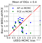
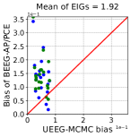
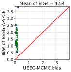
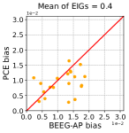
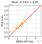
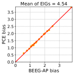
Figure 1: Top: the estimated biases of BEEG-AP and PCE versus those of UEEG-MCMC for 20 independent designs. Bottom: the estimated biases of PCE versus those of BEEG-AP for 20 independent designs.

A Toy Algebraic Model

In this experiment, we consider a toy problem with a single optimal design. The model is given by the following nonlinear map:

$$\bigg{[}\begin{matrix}y_{1}\\ y_{2}\end{matrix}\bigg{]}\!\!=\!\!\bigg{[}\begin{matrix}0.5\theta^{3}d_{1}+\theta\exp(-|0.2-0.5d_{1}|)+d_{1}^{2}\\ 0.5\theta^{3}(d_{2}\!+\!1.6)\!+\!\theta\exp(-|0.6\!+\!\!0.5d_{2}|)\!+\!d_{2}^{2}\end{matrix}\bigg{]}\!+\!\bigg{[}\begin{matrix}\epsilon_{1}\\ \epsilon_{2}\end{matrix}\bigg{]},$$ (25)

where $\theta$ is the model parameter, $d_{i}$ are design variables and $\epsilon_{i}$ are independent observation noises. We assign a uniform prior $\theta\sim\mathrm{Unif}(0,1)$ on the parameter and restrict the design variables in the interval of $[0,1]$. We conduct two experiments with different noise terms, i.e., a large noise scenario with $\epsilon_{i}\sim\mathcal{N}(0,(0.1)^{2})$ and a small noise scenario with $\epsilon_{i}\sim\mathcal{N}(0,(0.0001)^{2})$. By setting different noise terms, we can create scenarios to represent the small and large EIG cases and observe how the different methods perform under these conditions.

We applied five methods to this problem: BEEG-AP, UEEG-MCMC, ACE, PCE and GradBED. To mitigate the impact of randomness, we perform 20 independent runs for each method. The results for both the large and small noise settings are depicted in Fig. 2. From the figures we can see the final designs obtained by BEEG-AP and UEEG-MCMC are more concentrated compared to the designs generated by the other three methods. In particular, in the small noise case, UEEG-MCMC stands out as the only method where all designs eventually concentrate on a single point. Then we use different metrics to judge the quality of the designs obtained for the two settings. In the large noise case, we apply NMC with large samples to obtain high-quality estimations of the EIGs. Fig. 4 shows the estimated EIGs throughout the entire design space. Remarkably, we observe that the only optimal design identified by the estimations aligns with the the results obtained by BEEG-AP and UEEG-MCMC. In the small noise case, utilizing NMC for reliable EIG estimations becomes impractical due to the large simulation budget required. We therefore resort to using the posterior entropy as the metric to evaluate the quality of the designs, and the results are plotted in Fig. 4. From the figure, it is evident that BEEG-AP and UEEG-MCMC produce designs with smaller posterior entropy. Specifically, UEEG-MCMC yields even smaller posterior entropy than BEEG-AP, which demonstrates the superior performance of UEEG-MCMC in large EIG case.

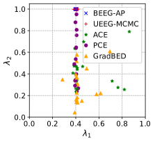
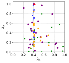
Figure 2: The final designs of 20 independent trials for large noise setting (left) and small noise setting (right).

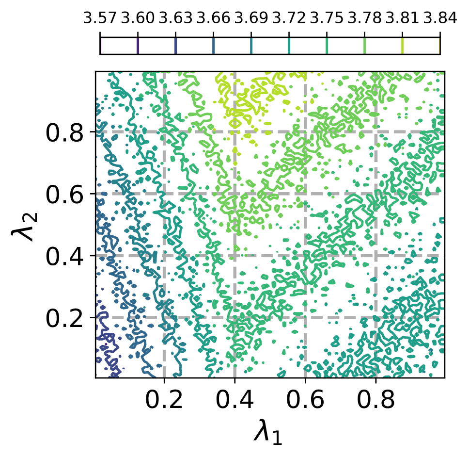
Figure 3: Estimates of EIG for large noise setting.

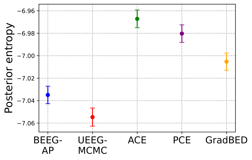
Figure 4: The posterior entropy for small noise setting. Shown are the means of entropy with their standard error bars.

Pharmacokinetic (PK) Model

Next, we consider an experimental design problem for PK studies. These studies aim to comprehend the underlying kinetics of a drug, shedding light on how it is absorbed, distributed, metabolized, and eliminated within the body over time. To achieve this understanding, it is a common practice to collect blood samples from the study subjects. However, the process of blood sampling involves various practical constraints, including financial limitations, participant burden, and ethical considerations. Therefore, researchers must strategically design the sampling strategy to gather meaningful information while minimizing the number of blood samples required. Here, we focus on the PK model introduced by (Ryan et al. 2014). The model under consideration consists of three parameters of interest ${\theta}=(k_{a},k_{e},V)$: the absorption rate constant $k_{a}$, the elimination rate constant $k_{e}$, and the volume of distribution V which represents the theoretical volume that the drug would need to occupy to achieve the current concentration in the blood plasma. The drug concentration of blood sample taken at time $t$, denoted as $y_{t}$, follows

$$y_{t}=\frac{D}{V}\cdot\frac{k_{a}}{k_{a}-k_{e}}\cdot(e^{-k_{e}t}-e^{-k_{a}t})\cdot(1+\epsilon_{1t})+\epsilon_{2t},$$ (26)

where $D=400$ is the fixed dose administered at the beginning of the experiment, $\epsilon_{1t}$ and $\epsilon_{2t}$ are the multiplicative and additive Gaussian noises respectively. As in (Ryan et al. 2014), we assign a log-normal prior on $\theta$

$$\log\theta\sim N\left[\left(\begin{array}[]{c}\log(1)\\ \log(0.1)\\ \log(20)\end{array}\right),\left(\begin{array}[]{ccc}0.05&0&0\\ 0&0.05&0\\ 0&0&0.05\end{array}\right)\right].$$ (27)

The design variables are assumed to be the 10 blood sampling times $(d_{1},...,d_{10})$, $d_{i}\geq 0$ for $i=1,...,10$, and the corresponding drug concentrations at these times $(y_{d_{1}},...,y_{d_{10}})$ form the observations.

Again, we create a small EIG setting with $\epsilon_{1t}\sim\mathcal{N}(0,0.01)$ and $\epsilon_{2t}\sim\mathcal{N}(0,0.1)$, and a large EIG setting with $\epsilon_{1t}=0$ and $\epsilon_{2t}\sim\mathcal{N}(0,0.001)$. In small EIG scenario we use large samples to compute high-quality NMC estimations to validate various methods, while in large EIG scenario we compare the posterior entropies obtained by them. Fig. 6 shows BEEG-AP outperforms other methods in terms of convergence rate in small EIG scenario. This can also be supported by examining the convergence histories of all methods, as shown in Fig. B.1 in the Appendix. However, in large EIG scenario, UEEG-MCMC achieve the best performance as the validation experiments indicate in Fig. 6 and the convergence histories show in Fig. B.2 in the Appendix. It should be mentioned that in this case ACE fails to learn a posterior inference network due to the strong dependencies between the observations and the parameters.

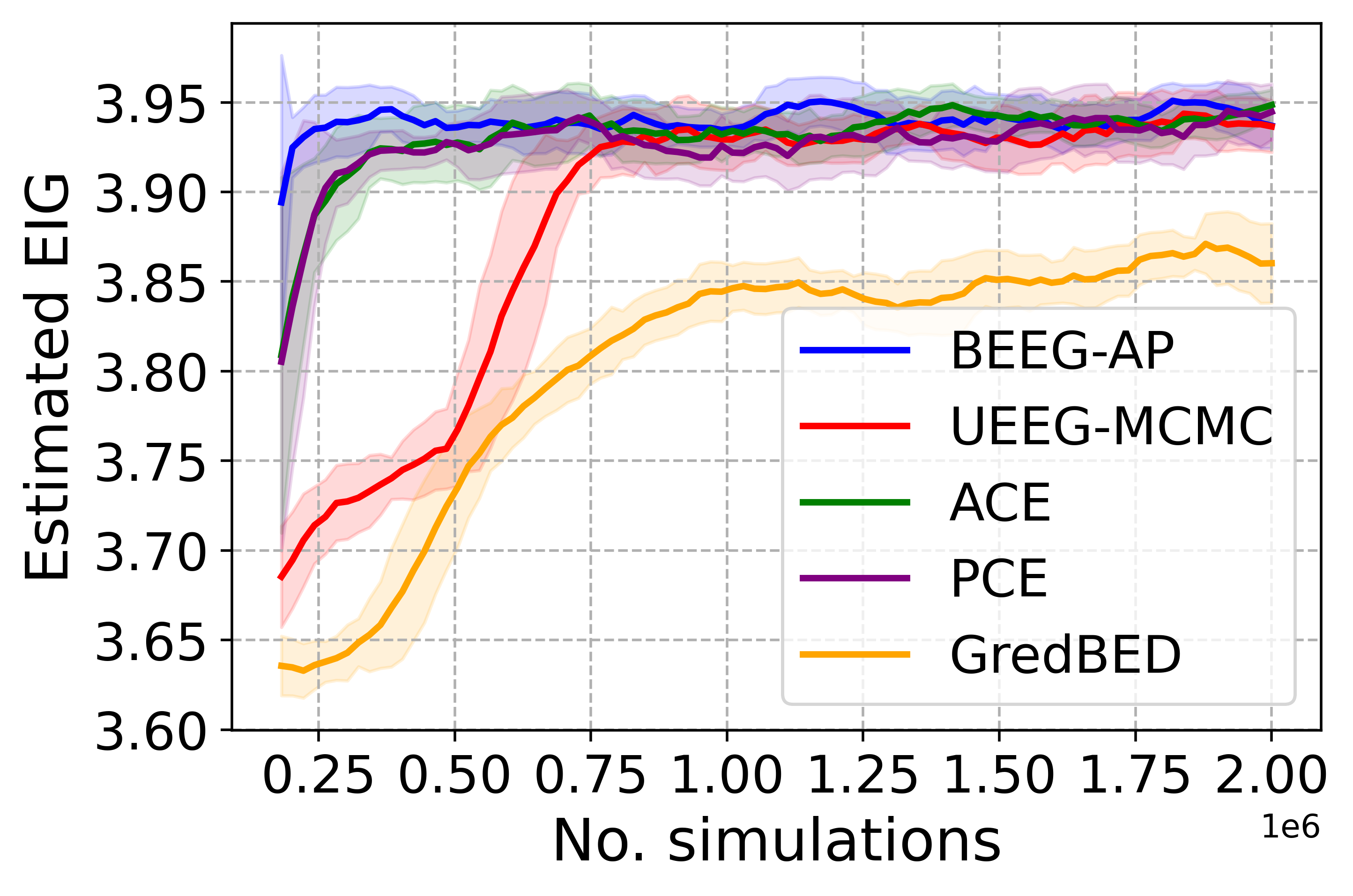
Figure 5: Optimization of EIG for PK model with multiplicative noise $\mathcal{N}(0,0.01)$ and additive noise $\mathcal{N}(0,0.1)$ as a function of number of simulations. Shown are the moving averages with the standard error bars.

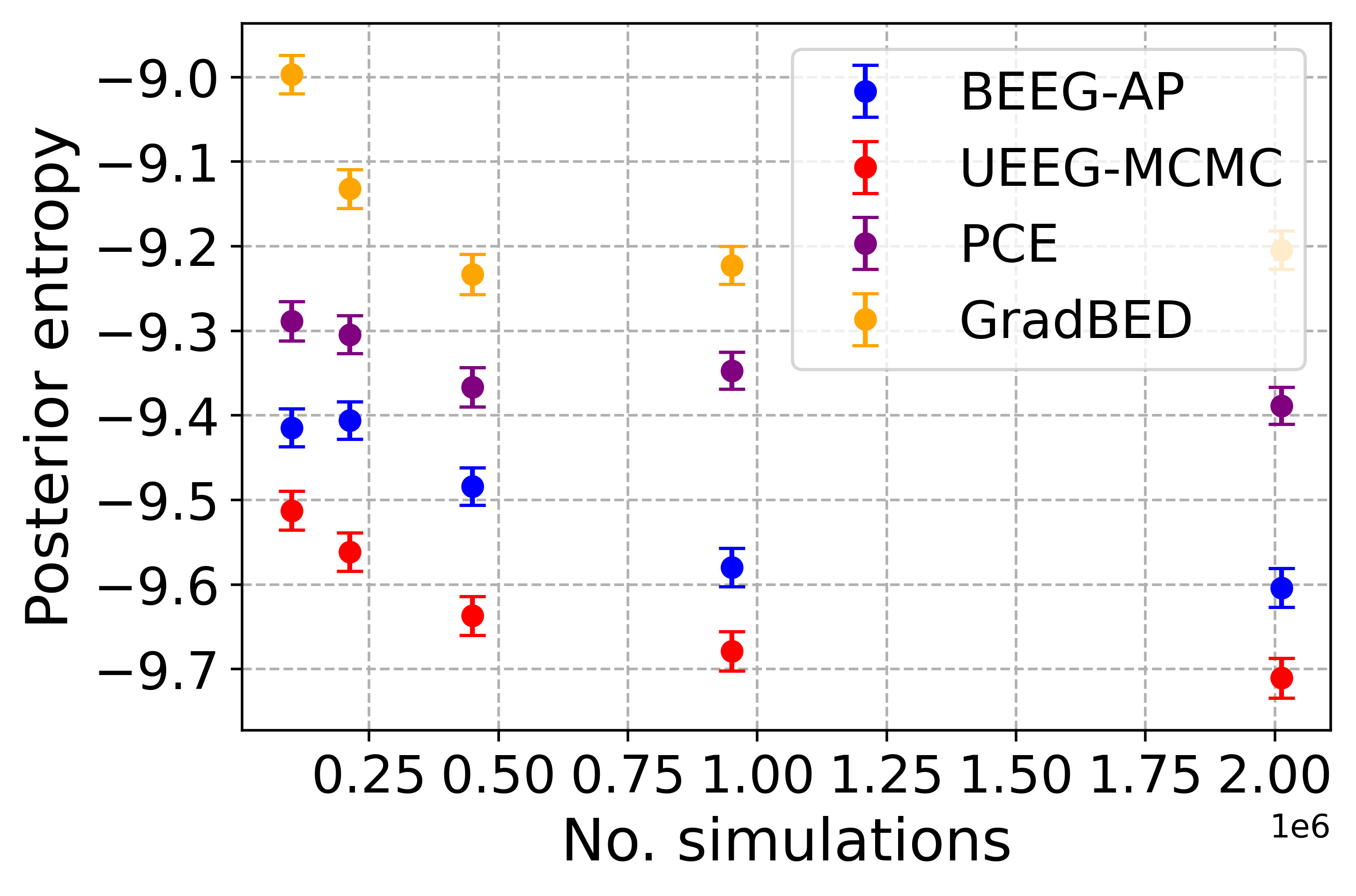
Figure 6: The posterior entropy for PK model with additive noise $\mathcal{N}(0,0.001)$ as a function of number of simulations. Shown are the means of entropy with their standard error bars.
 

Signal Transducer and Activator of Transcription 5 (STAT5) model

Finally we aim to design the measurement times for a dynamic system modeled by ordinary differential equations (ODEs). We take the mathematical model of the core module of the Janus family of kinases (JAK)–signal transducer and activator of transcription (STAT) pathway in (Swameye et al. 2003) as a case study. The core module of the JAK-STAT pathway is represented by the latent transcription factor STAT5, and the dynamics of STAT5 populations $x_{1}$, $x_{2}$, $x_{3}$ and $x_{4}$ can be described by four coupled ODEs (see Appendix for full details of the ODEs). The rate constants $k_{1}$, $k_{2}$ and the delay parameter $\tau$ are the three model parameters to be inferred from measured data.

It is experimentally challenging to directly measure distinct STAT5 populations separately. Instead, one can measure the amount of tyrosine phosphorylated STAT5 $y_{1}=s_{1}(x_{2}+x_{3})$ and the total amount of STAT5 $y_{2}=s_{2}(x_{1}+x_{2}+x_{3})$. We assume the scaling parameters to be $s_{1}=0.33$ and $s_{2}=0.26$. We assign a uniform prior on $\theta=(k_{1},k_{2},\tau)$ with lower range $[0.5,0.05,4.0]$ and upper range $[3.0,0.2,10.0]$. The objective of the experimental design is to allocate 16 measurement times for STAT5 populations over a time span from 0 to 60 minutes, which yields 32 experimental measurements in total.

In this application, we set two levels of additive Gaussian observation noises, $\mathcal{N}(0,10^{-4})$ and $\mathcal{N}(0,10^{-6})$, representing the small and large EIG scenarios respectively. In both cases, we assess the quality of designs by the posterior entropies obtained. The results for the small EIG scenario depicted in Fig. 8 indicate that, both BEEG-AP and UEEG-MCMC outperform other methods and BEEG-AP appears the best. However, UEEG-MCMC demonstrates the best performance in the large EIG scenario, while BEEG-AP’s performance falls below that of GradBED, as shown in Fig. 8. ACE fails in both scenario. The convergence histories of all approaches can be found in Fig. B.3 and Fig. B.4 in the Appendix.

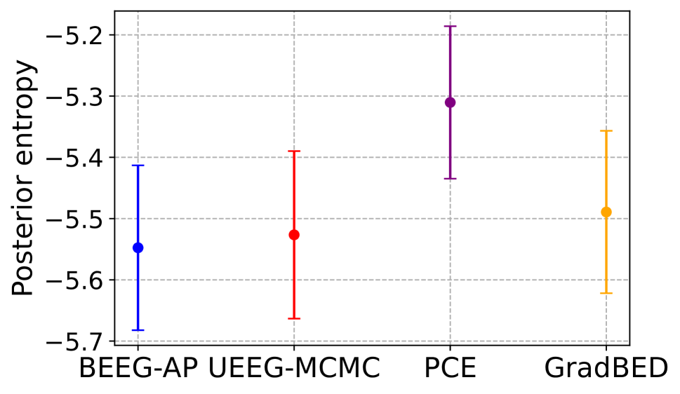
Figure 7: The posterior entropy for STAT5 model with additive noise $\mathcal{N}(0,10^{-4})$ for designs obtained. Shown are the means of entropy with their standard error bars.

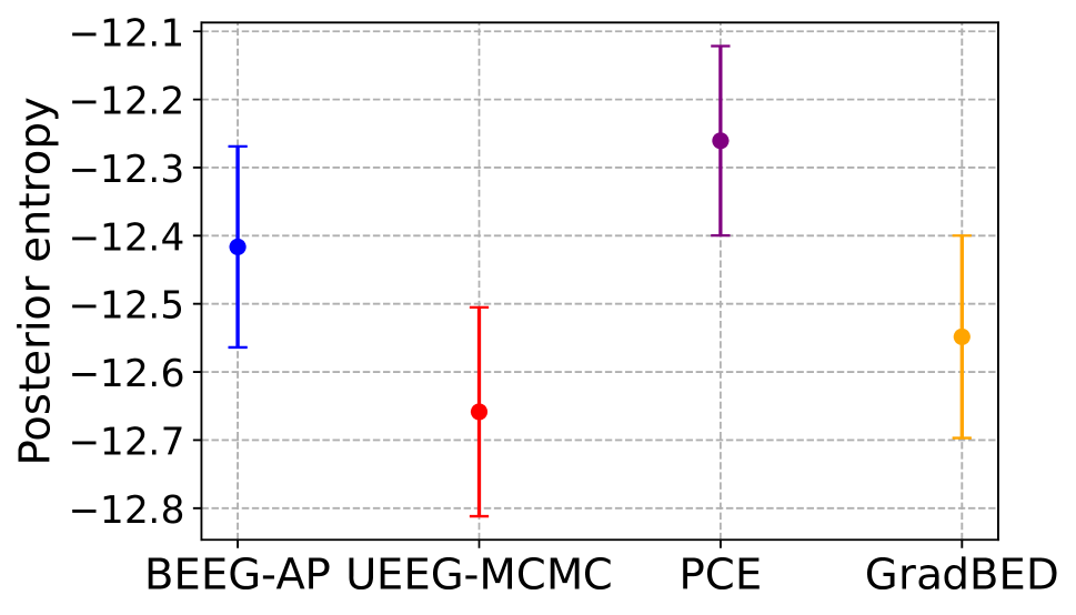
Figure 8: The posterior entropy for STAT5 model with additive noise $\mathcal{N}(0,10^{-6})$ for designs obtained. Shown are the means of entropy with their standard error bars.

Conclusion

In this work we have proposed two approaches, UEEG-MCMC and BEEG-AP, to Bayesian experimental design based on EIG gradient estimation. We use MCMC sampling techniques to build the gradient estimation for UEEG-MCMC, while BEEG-AP approximates the EIG gradients with atomic priors. Both of them are straightforward to implement and have demonstrated improved performance compared to bench-marking methods.

Our theoretical analysis aligns well with the numerical results. Specifically, BEEG-AP exhibits superior simulation efficiency when dealing with problems that have small ground-truth EIG values, making it a favorable option in such cases. On the other hand, UEEG-MCMC shows robustness across various EIG levels, making it suitable for a broader range of experimental scenarios. We believe the work provides researchers and practitioners with promising tools and guidance to optimize their experiments and make informed decisions across different domains.

Appendix A Proofs of Results

Lemma 1.

The gradient of the logarithm of the marginal density w.r.t. the experimental condition $\lambda$ admits the following representation:

$$\nabla_{\lambda}\log p(g(\theta,\epsilon,\lambda))|\lambda)=-\mathbb{E}_{q(\theta^{\prime}|g(\theta,\epsilon,\lambda),\lambda)}[\nabla_{\lambda}\log l(g(\theta,\epsilon,\lambda)|\theta^{\prime},\lambda)],$$ (A.1)

where $q(\theta^{\prime}|y,\lambda)\propto\pi_{\mathrm{\theta}}(\theta^{\prime})l(y|\theta^{\prime},\lambda)$ is the posterior density of parameters given the observation sample $y$.

Proof.

Let $y=g(\theta,\epsilon,\lambda)$, we find

$$\nabla_{\lambda}\log p(g(\theta,\epsilon,\lambda)|\lambda)$$ (A.2)

$$= \nabla_{\lambda}\log p(y|\lambda)$$

$$= \frac{1}{p(y|\lambda)}\nabla_{\lambda}p(y|\lambda)$$

$$= \frac{1}{p(y|\lambda)}\nabla_{\lambda}\int\pi_{\mathrm{\theta}}(\theta^{\prime})l(y|\theta^{\prime},\lambda)d\theta^{\prime}$$

$$= \frac{1}{p(y|\lambda)}\int\pi_{\mathrm{\theta}}(\theta^{\prime})\nabla_{\lambda}l(y|\theta^{\prime},\lambda)d\theta^{\prime}$$

$$= \int{q(\theta^{\prime}|y,\lambda)}\frac{\nabla_{\lambda}l(y|\theta^{\prime},\lambda)}{l(y|\theta^{\prime},\lambda)}d\theta^{\prime}$$

$$= \int{q(\theta^{\prime}|y,\lambda)}\nabla_{\lambda}\log l(y|\theta^{\prime},\lambda)d\theta^{\prime}$$

$$= \mathbb{E}_{q(\theta^{\prime}|y,\lambda)}[\nabla_{\lambda}\log l(y|\theta^{\prime},\lambda)],$$

Finally, by plugging $y=g(\theta,\epsilon,\lambda)$ back into the equation, we obtain

$$\nabla_{\lambda}\log p(g(\theta,\epsilon,\lambda)|\lambda)=\mathbb{E}_{q(\theta^{\prime}|g(\theta,\epsilon,\lambda),\lambda)}[\nabla_{\lambda}\log l(g(\theta,\epsilon,\lambda)|\theta^{\prime},\lambda)].$$ (A.3)

∎

Theorem 1.

The gradient of the entropy $H(p(y|\lambda))$ w.r.t. the experimental condition $\lambda$ satisfies

$$\nabla_{\lambda}H(p(y|\lambda))=-\mathbb{E}_{\pi_{\mathrm{\theta}}(\theta)\pi_{\mathrm{\epsilon}}(\epsilon)q(\theta^{\prime}|g(\theta,\epsilon,\lambda),\lambda)}[\nabla_{\lambda}\log l(g(\theta,\epsilon,\lambda)|\theta^{\prime},\lambda)],$$ (A.4)

where $q(\theta^{\prime}|y,\lambda)\propto\pi_{\mathrm{\theta}}(\theta^{\prime})l(y|\theta^{\prime},\lambda)$ is the posterior density of parameters given the observation sample $y$.

Proof.

By the reparameterization trick, we have

$$\nabla_{\lambda}H(p(y|\lambda)) =-\nabla_{\lambda}\mathbb{E}_{\pi_{\mathrm{\theta}}(\theta)\pi_{\mathrm{\epsilon}}(\epsilon)}[\log p(g(\theta,\epsilon,\lambda)|\lambda)]$$ (A.5)

$$=-\mathbb{E}_{\pi_{\mathrm{\theta}}(\theta)\pi_{\mathrm{\epsilon}}(\epsilon)}[\nabla_{\lambda}\log p(g(\theta,\epsilon,\lambda)|\lambda)].$$

Using Lemma 1, we can substitute the gradient of the logarithm of the marginal density in the above equation by the posterior expectation of the logarithm of the likelihood function. ∎

Corollary 1.

The gradient of the EIG $U(\lambda)$ w.r.t. the experimental condition $\lambda$ satisfies

$$\nabla_{\lambda}U(\lambda)=\mathbb{E}_{\pi_{\mathrm{\theta}}(\theta)\pi_{\mathrm{\epsilon}}(\epsilon)q(\theta^{\prime}|g(\theta,\epsilon,\lambda),\lambda)}[\nabla_{\lambda}\log l(g(\theta,\epsilon,\lambda)|\theta,\lambda)-\nabla_{\lambda}\log l(g(\theta,\epsilon,\lambda)|\theta^{\prime},\lambda)],$$ (A.6)

where $q(\theta^{\prime}|y,\lambda)\propto\pi_{\mathrm{\theta}}(\theta^{\prime})l(y|\theta^{\prime},\lambda)$ is the posterior density of parameters given the observation sample $y$.

Proof.

Applying the reparameterization trick to the gradient of the negative conditional entropy term $\mathbb{E}_{\pi_{\mathrm{\theta}(\theta)l(y|\theta,\lambda)}}[\log l(y|\theta,\lambda)]$ w.r.t. the experimental condition $\lambda$, we have

$$\nabla_{\lambda}\mathbb{E}_{\pi_{\mathrm{\theta}(\theta)l(y|\theta,\lambda)}}[\log l(y|\theta,\lambda)] =\mathbb{E}_{\pi_{\mathrm{\theta}}(\theta)\pi_{\mathrm{\epsilon}}(\epsilon)}[\nabla_{\lambda}\log l(g(\theta,\epsilon,\lambda)|\theta,\lambda)]$$ (A.7)

$$=\mathbb{E}_{\pi_{\mathrm{\theta}}(\theta)\pi_{\mathrm{\epsilon}}(\epsilon)q(\theta^{\prime}|g(\theta,\epsilon,\lambda),\lambda)}[\nabla_{\lambda}\log l(g(\theta,\epsilon,\lambda)|\theta,\lambda)].$$

Combining the above equation with Theorem 1, we finally get Eq. (A.6). ∎

Theorem 2.

The expectation of $\widehat{U}_{srNMC}^{M}(\lambda)$ satisfies the following:

1. $\mathbb{E}[\widehat{U}_{srNMC}^{M}(\lambda)]$ is a lower bound on $U(\lambda)$ for any $M>0$.

2. $\mathbb{E}[\widehat{U}_{srNMC}^{M}(\lambda)]$ is monotonically increasing in $M$, i.e., $\mathbb{E}[\widehat{U}_{srNMC}^{M_{1}}(\lambda)]\leq\mathbb{E}[\widehat{U}_{srNMC}^{M_{2}}(\lambda)]$ for $0\leq M_{1}\leq M_{2}$.

Proof.

To prove the first result in Theorem 2, we first note that the outer Monte Carlo terms are identically distributed. Thus,

$$\mathbb{E}[\widehat{U}_{srNMC}^{M}(\lambda)]=\mathbb{E}\Bigg{[}\log\frac{l(y^{(1)}|\theta^{(1)},\lambda)}{\frac{1}{M}\sum_{j=1}^{M}l(y^{(1)}|\theta^{(j)},\lambda)}\Bigg{]},$$ (A.8)

where $y^{(1)}=g(\theta^{(1)},\epsilon^{(1)},\lambda)$ and the expectation is taken over $p(y^{(1)}|\lambda)q(\theta^{(1)}|y^{(1)},\lambda)\prod_{j=2}^{M}\pi_{\mathrm{\theta}}(\theta^{(j)})$. We proceed the rest as in (Foster et al. 2020). We let $\delta=U(\lambda)-\mathbb{E}[\widehat{U}_{srNMC}^{M}(\lambda)]$, then

$$\delta =\mathbb{E}\Bigg{[}\log\frac{\frac{1}{M}\sum_{j=1}^{M}l(y^{(1)}|\theta^{(j)},\lambda)}{p(y^{(1)}|\lambda)}\Bigg{]}$$ (A.9)

$$=\mathbb{E}\Bigg{[}\log\frac{\frac{1}{M}\sum_{j=1}^{M}q(\theta^{(j)}|y^{(1)},\lambda)\prod_{k\neq j}\pi_{\mathrm{\theta}}(\theta^{(k)})}{\prod_{j=1}^{M}\pi_{\mathrm{\theta}}(\theta^{(j)})}\Bigg{]}$$

$$=\mathbb{E}\Bigg{[}\log\frac{P(\theta^{(1:M)}|y^{(1)})}{\prod_{j=1}^{M}\pi_{\mathrm{\theta}}(\theta^{(j)})}\Bigg{]},$$

where $P(\theta^{(1:M)}|y^{(1)})=\frac{1}{M}\sum_{j=1}^{M}q(\theta^{(j)}|y^{(1)},\lambda)\prod_{k\neq j}\pi_{\mathrm{\theta}}(\theta^{(k)})$. Due to the permutation symmetry of the integrand over the labels $1,...,M$, the expectation keeps the same if it is instead taken over $p(y^{(1)}|\lambda)P(\theta^{(1:M)}|y^{(1)})$. Thus we have

$$\delta=\mathbb{E}\bigg{[}\mathrm{D_{KL}}\bigg{(}P(\theta^{(1:M)}|y^{(1)})\|\prod_{j=1}^{M}\pi_{\mathrm{\theta}}(\theta^{(j)})\bigg{)}\bigg{]}\geq 0,$$ (A.10)

where the expectation is taken over $p(y^{(1)}|\lambda)$.

To prove the second result, as in the former proof we let $\phi=\mathbb{E}[\widehat{U}_{srNMC}^{M_{2}}(\lambda)]-\mathbb{E}[\widehat{U}_{srNMC}^{M_{1}}(\lambda)]$. Then

$$\phi =\mathbb{E}\Bigg{[}\log\frac{\frac{1}{M_{1}}\sum_{j=1}^{M_{1}}l(y^{(1)}|\theta^{(j)},\lambda)}{\frac{1}{M_{2}}\sum_{j=1}^{M_{2}}l(y^{(1)}|\theta^{(j)},\lambda)}\Bigg{]}$$ (A.11)

$$=\mathbb{E}\Bigg{[}\log\frac{Q(\theta^{(1:M_{2})}|y^{(1)})}{P(\theta^{(1:M_{2})}|y^{(1)})}\Bigg{]},$$

where the expectation is taken over $p(y^{(1)}|\lambda)q(\theta^{(1)}|y^{(1)},\lambda)\prod_{j=2}^{M_{2}}\pi_{\mathrm{\theta}}(\theta^{(j)})$ and $Q(\theta^{(1:M_{2})}|y^{(1)})=\frac{1}{M_{1}}\sum_{j=1}^{M_{1}}q(\theta^{(j)}|y^{(1)},\lambda)\prod_{k\neq j}^{M_{2}}\pi_{\mathrm{\theta}}(\theta^{(k)})$. Again, using the permutation symmetry, we can get the same expectation if the sampling distribution is taken as $p(y^{(1)}|\lambda)Q(\theta^{(1:M_{2})}|y^{(1)})$ instead. Thus,

$$\phi=\mathbb{E}\bigg{[}\mathrm{D_{KL}}\bigg{(}Q(\theta^{(1:M_{2})}|y^{(1)})\|P(\theta^{(1:M_{2})}|y^{(1)})\bigg{)}\bigg{]}\geq 0,$$ (A.12)

where the expectation is taken over $p(y^{(1)}|\lambda)$. ∎

Theorem 3.

If $l(g(\theta,\epsilon,\lambda)|\theta^{\prime},\lambda)$ is bounded away from 0 and uniformly bounded from above (i.e., $C_{1}\leq l(g(\theta,\epsilon,\lambda)|\theta^{\prime},\lambda)\leq C_{2}$ a.s. for some positive constants $C_{1}$ and $C_{2}$), then the mean squared error of $\widehat{U}_{srNMC}^{M}(\lambda)$ converges to 0 at rate $O(1/M)$.

Proof.

For simplicity, we denote $f(\theta,\epsilon)=\log\frac{l(g(\theta,\epsilon,\lambda)|\theta,\lambda)}{p(g(\theta,\epsilon,\lambda)|\lambda)}$. Then the ground-truth EIG can be represented as $U(\lambda)=\mathbb{E}[f(\theta,\epsilon)]$. Using Minkowski’s inequality, the mean squared error of $\widehat{U}_{srNMC}^{M}(\lambda)$ can be bounded by

$$\mathbb{E}[(U(\lambda)-\widehat{U}_{srNMC}^{M}(\lambda))^{2}]=\lVert U(\lambda)-\widehat{U}_{srNMC}^{M}(\lambda)\rVert^{2}_{2}\leq U^{2}+V^{2}+2UV\leq 2(U^{2}+V^{2}),$$ (A.13)

where the expectation is taken over $\prod_{i=1}^{M}\pi_{\mathrm{\theta}}(\theta^{(i)})\pi_{\mathrm{\epsilon}}(\epsilon^{(i)})$ , $U=\Big{\lVert}U(\lambda)-\frac{1}{M}\sum_{i=1}^{M}f(\theta^{(i)},\epsilon^{(i)})\Big{\rVert}_{2}$ and $V=\Big{\lVert}\frac{1}{M}\sum_{i=1}^{M}f(\theta^{(i)},\epsilon^{(i)})-\widehat{U}_{srNMC}^{M}(\lambda)\Big{\rVert}_{2}$. Since $l(g(\theta,\epsilon,\lambda)|\theta^{\prime},\lambda)$ is uniformly bounded from below and above, we have $f\in L^{2}$. Also noting that $U$ is the square of mean error of a Monte Carlo estimation, it is easy to get $U=O(1/\sqrt{M})$. Now we turn to bound $V$. Using the assumption that $l(g(\theta,\epsilon,\lambda)|\theta^{\prime},\lambda)\geq C_{1}$ a.s., we have

$$V =\Big{\lVert}\frac{1}{M}\sum_{i=1}^{M}\log\frac{\frac{1}{M}\sum_{j=1}^{M}l(y^{(i)}|\theta^{(j)},\lambda)}{p(y^{(i)}|\lambda)}\Big{\rVert}_{2}$$ (A.14)

$$\leq\frac{1}{M}\sum_{i=1}^{M}\Big{\lVert}\log\frac{\frac{1}{M}\sum_{j=1}^{M}l(y^{(i)}|\theta^{(j)},\lambda)}{p(y^{(i)}|\lambda)}\Big{\rVert}_{2}$$

$$\leq\frac{1}{C_{1}M}\sum_{i=1}^{M}\Big{\lVert}{\frac{1}{M}\sum_{j=1}^{M}l(y^{(i)}|\theta^{(j)},\lambda)}-{p(y^{(i)}|\lambda)}\Big{\rVert}_{2},$$

where $y^{(i)}=g(\theta^{(i)},\epsilon^{(i)},\lambda)$. For each term of the above equation, by Minkowski’s inequality we have

$$\Big{\lVert}{\frac{1}{M}\sum_{j=1}^{M}l(y^{(i)}|\theta^{(j)},\lambda)}-{p(y^{(i)}|\lambda)}\Big{\rVert}_{2}$$ (A.15)

$$\leq \frac{1}{M}\Big{\lVert}l(y^{(i)}|\theta^{(i)},\lambda)-l(y^{(i)}|\theta^{\prime(i)},\lambda)\Big{\rVert}_{2}+\Big{\lVert}{\frac{1}{M}\sum_{j\neq i}^{M}l(y^{(i)}|\theta^{(j)},\lambda)}+\frac{1}{M}l(y^{(i)}|\theta^{\prime(i)},\lambda)-{p(y^{(i)}|\lambda)}\Big{\rVert}_{2},$$

where $\theta^{\prime(i)}\sim\pi_{\theta}(\theta)$. Using the assumption that $l(g(\theta,\epsilon,\lambda)|\theta^{\prime},\lambda)\leq C_{2}$, the first term of above equation can be bounded by $2C_{2}/M$. The square of the second equation can be bounded as

$$\Big{\lVert}{\frac{1}{M}\sum_{j\neq i}^{M}l(y^{(i)}|\theta^{(j)},\lambda)}+\frac{1}{M}l(y^{(i)}|\theta^{\prime(i)},\lambda)-{p(y^{(i)}|\lambda)}\Big{\rVert}_{2}^{2}$$ (A.16)

$$= \mathbb{E}\Big{[}\mathbb{E}\Big{[}\Big{(}{\frac{1}{M}\sum_{j\neq i}^{M}l(y^{(i)}|\theta^{(j)},\lambda)}+\frac{1}{M}l(y^{(i)}|\theta^{\prime(i)},\lambda)-{p(y^{(i)}|\lambda)}\Big{)}^{2}\Big{|}y^{(i)}\Big{]}\Big{]}$$

$$= \mathbb{E}\Big{[}\mathrm{Var}\Big{[}{\frac{1}{M}\sum_{j\neq i}^{M}l(y^{(i)}|\theta^{(j)},\lambda)}+\frac{1}{M}l(y^{(i)}|\theta^{\prime(i)},\lambda)\Big{|}y^{(i)}\Big{]}\Big{]}$$

$$= \frac{1}{M}\mathbb{E}\Big{[}\mathrm{Var}\Big{[}l(y^{(i)}|\theta^{\prime(i)},\lambda)\Big{|}y^{(i)}\Big{]}\Big{]}$$

where the first equality is obtained by the tower property of conditional expectation. It can be further bounded $O(1/M)$ noting that $l(y^{(i)}|\theta^{\prime(i)},\lambda)$ is uniformly bounded from below and above. Therefore, we have $V=O(1/\sqrt{M})$ as well. Finally, using the obtained bounds of $U$ and $V$ we get the mean squared error of $\widehat{U}_{srNMC}^{M}(\lambda)$

$$\mathbb{E}[(U(\lambda)-\widehat{U}_{srNMC}^{M}(\lambda))^{2}]\leq 2(U^{2}+V^{2})=O(1/M).$$ (A.17)

∎

Theorem 4.

For any $C$ satisfying $0\leq C\leq U(\lambda)/2$, if $M\leq\exp(U(\lambda)/2)$, we have

$$U(\lambda)-\widehat{U}_{srNMC}^{M}(\lambda)>C.$$ (A.18)

Proof.

We first show that $\widehat{U}_{srNMC}^{M}(\lambda)$ does not exceed $\log M$. By the definition of srNMC, we have

$$\widehat{U}_{srNMC}^{M}(\lambda) =\frac{1}{M}\sum_{i=1}^{M}\log\frac{l(y^{(i)}|\theta^{(i)},\lambda)}{\frac{1}{M}\sum_{j=1}^{M}l(y^{(i)}|\theta^{(j)},\lambda)}$$ (A.19)

$$\leq\frac{1}{M}\sum_{i=1}^{M}\log\frac{l(y^{(i)}|\theta^{(i)},\lambda)}{\frac{1}{M}l(y^{(i)}|\theta^{(i)},\lambda)}$$

$$\leq\frac{1}{M}\sum_{i=1}^{M}\log M=\log M,$$

where $y^{(i)}=g(\theta^{(i)},\epsilon^{(i)},\lambda)$. Using this inequality and $M\leq\exp(U(\lambda)/2)$, it is easy to get

$$U(\lambda)-\widehat{U}_{srNMC}^{M}(\lambda) \geq U(\lambda)-\log M$$ (A.20)

$$\geq U(\lambda)/2\geq C.$$

∎

Appendix B Further details of experiments

B.1 EIG Gradient Estimation Accuracy

We assume 3 design variables (i.e. $\lambda=(\lambda_{1},\lambda_{2},\lambda_{3})$) for this test. The 20 independent designs are uniformly drawn from $[-1,1]^{3}$. To estimate the biases associated with the methods under investigation, we perform 100 independent trials. Table 1 summarizes the number of samples used to estimate the gradient for a single design.

Method	Number of samples
BEEG-AP	$100\times 100(M)$
UEEG-MCMC	$100\times 100(L)$
PCE	$100\times 100(M)\times(100(N)+1)$

Table 1: Method and number of samples for the test of EIG gradient estimation accuracy.

B.2 A Toy Algebraic Model

In this test, we allocate a simulation budget of $2\times 10^{4}$ for optimizing the design variables for each method. For UEEG-MCMC, we use slice sampling (Neal 2003) with a thinning factor of 2 to draw 10 samples for the posterior sampling in Eq. (14). For ACE, we use a conditional Gaussian posterior inference network $q_{\phi}(\cdot|y)=\mathrm{normpdf}(\cdot|\mu_{\phi}(y),e^{2\sigma_{\phi}(y)})$, where $\mu_{\phi}$ and $\sigma_{\phi}$ are the two outputs of a two-layer fully connected network with 50 hidden units and ReLU activation functions. For GradBED, we use a two-layer fully connected network $T_{\psi}$ with 50 hidden units and ReLU activation functions. The number of samples used to estimate a single gradient for each method is given by Table 3.

Method	Number of samples
BEEG-AP	$100(M)$
UEEG-MCMC	$10(M)\times\mathrm{No.~{}samples~{}from~{}slice~{}sampling}$
ACE	$10(M)\times(10(N)+1)$
PCE	$10(M)\times(10(N)+1)$
GradBED	$100(M)$

Table 2: Method and number of samples for the toy model.

To validate the quality of designs, we use NMC with 10,000 samples for each estimate of EIG in Fig. 4. The estimated posterior entropy in Fig. 4 is obtained as follows. In our experimental setup, each method yields 20 final designs. For each of these designs, we conduct simulations resulting in 500 observed data points derived from the marginal likelihood, thus forming 500 guess posteriors. Subsequently, kernel density estimation (KDE) is applied to these posteriors, utilizing 100 posterior samples for each, to approximate the entropies of these posteriors. The posterior entropy for each method is then computed by averaging these approximated entropies.

B.3 PK Model

In this application, we allocate a simulation budget of $2\times 10^{6}$ for optimizing the design variables for each method. For UEEG-MCMC, we use an adaptive Metropolis-Hastings (MH) method with a thinning factor of 95 to draw only one sample for the posterior sampling in Eq. (14). For ACE, we utilize the Mixture Density Network (Bishop 1994) as our chosen posterior inference network, with 3 hidden layers, 50 hidden units in each layer and ReLU activation function. For GradBED, we follow the network settings in (Kleinegesse and Gutmann 2020). Specifically, we use a one-layer connected network $T_{\psi}$ consisting of 300 hidden units and ReLU activation functions. The number of samples used to estimate a single gradient for each method is given by Table 3.

Method	Number of samples
BEEG-AP	$100(M)$
UEEG-MCMC	$1(M)\times 100(\mathrm{approximated~{}cost~{}of~{}the~{}adaptive~{}MH}$)
ACE	$10(M)\times(10(N)+1)$
PCE	$10(M)\times(10(N)+1)$
GradBED	$100(M)$

Table 3: Method and number of samples for PK model and STAT5 model.

In the validation experiments, we use NMC with 10,000 samples for each estimate of EIG in Fig. 6. In Fig. 6, the posterior entropy for each method is estimated via 1000 independent trials (see Appendix B.2 for the procedure). For each trial, we use KDE to estimate the guess posterior entropy with 1000 samples.

B.4 STAT5 Model

The dynamics of STAT5 populations can be described by four coupled ODEs

$$\dot{x}_{1}=-k_{1}x_{1}\operatorname{EpoR}_{A}(t)+k_{2}x_{3}(t-\tau)$$ (B.1)

$$\dot{x}_{2}=-x_{2}^{2}+k_{1}x_{1}\operatorname{EpoR}_{A}(t)$$

$$\dot{x}_{3}=-k_{2}x_{3}+x_{2}^{2}$$

$$\dot{x}_{4}=-k_{2}x_{3}(t-\tau)+k_{2}x_{3}.$$

The variables in the model are defined as follows. $x_{1}$ represents unphosphorylated STAT5. $x_{2}$ and $x_{3}$ represent tyrosine phosphorylated monomeric STAT5 and tyrosine phosphorylated dimeric STAT5 respectively. $x_{4}$ is the nuclear STAT5. $\operatorname{EpoR}_{A}(t)$ describes the erythropoietin receptor activity that determines the STAT5 response.

We assume that $x_{1}(0)=3.71$ is the only non-zero initial state of the ODES. To facilitate the solvability of the ordinary differential equations (ODEs), as in (Peifer and Timmer 2007; Banga and Balsa-Canto 2008), we apply linear interpolation to synthesize the function $\operatorname{EpoR}_{A}(t)$ with the original data in (Swameye et al. 2003), and use a delay chain of length $N$ to approximate the delayed term $x_{3}(t-\tau)$,

$$\begin{gathered}\dot{q}_{1}=\frac{N}{\tau}\left(\operatorname{in}(t)-q_{1}\right)\\ \dot{q}_{2}=\frac{N}{\tau}\left(q_{1}-q_{2}\right)\\ \ldots\\ \dot{q}_{N-1}=\frac{N}{\tau}\left(q_{N-2}-q_{N-1}\right)\\ \text{ out }=\frac{N}{\tau}\left(q_{N-1}-\operatorname{out}(t)\right),\end{gathered}$$ (B.2)

where $N=8$, $\operatorname{in}(t)=x_{3}(t)$ and $\operatorname{out}(t)=x_{3}(t-\tau)$.

To build the sampling path that supports backpropagation through ODE solutions, we utilize the package torchdiffeq (Chen et al. 2018) to solve the ODEs with 3/8-Runge-Kutta method (Butcher 1996). Linear interpolation is then applied to get the observations at any measurement times.

In this application, we allocate a simulation budget of $5\times 10^{5}$ for optimizing the design variables for each method. The settings for the methods involved are consistent with those employed for the PK model, and the sample size for each method is also provided in Table 3. In the validation experiments, the posterior entropy for each method shown in Fig. 8 and Fig. 8 is estimated via 100 independent trials (see Appendix B.2 for the procedure). For each trial, KDE is employed with 1000 posterior samples.

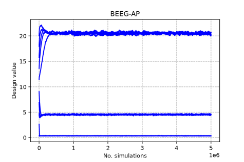
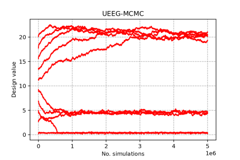
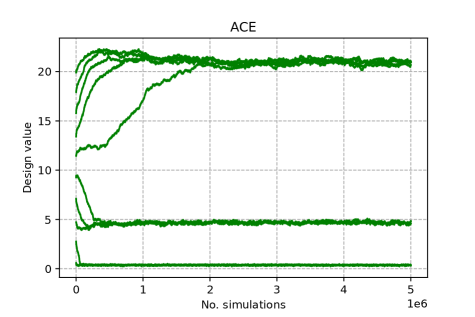
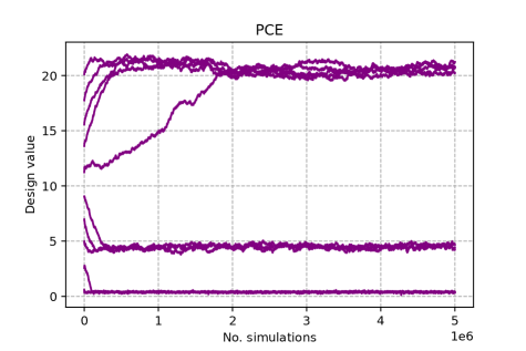
Figure B.1: Convergence of the individual design dimensions for PK model with multiplicative noise $\mathcal{N}(0,0.01)$ and additive noise $\mathcal{N}(0,0.1)$.

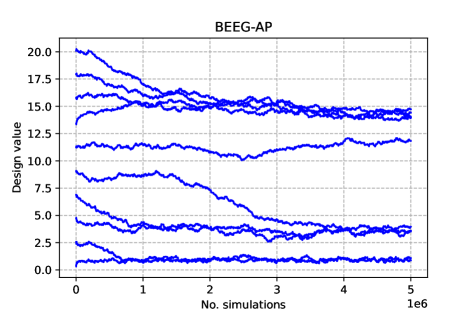
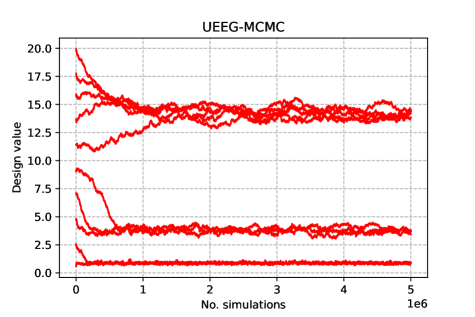
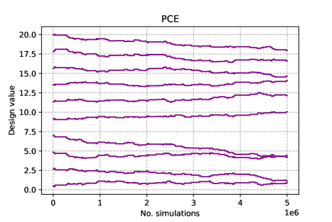
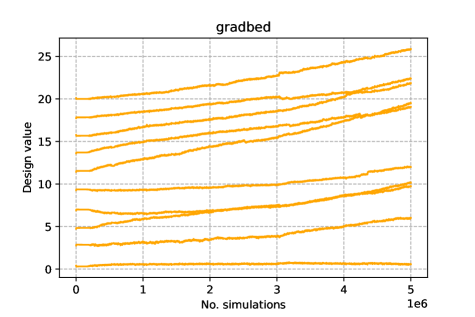
Figure B.2: Convergence of the individual design dimensions for PK model with additive noise $\mathcal{N}(0,0.001)$.

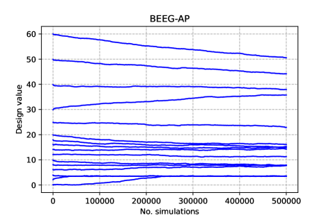
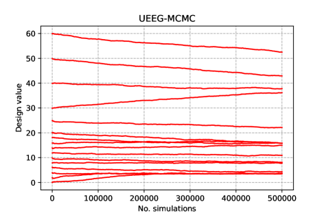
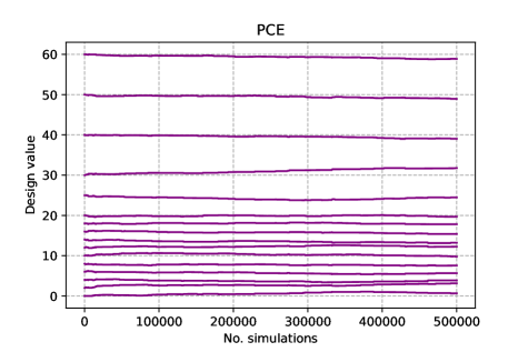
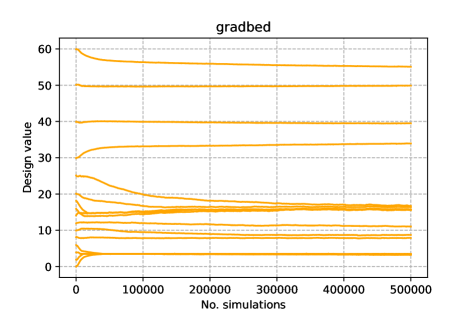
Figure B.3: Convergence of the individual design dimensions for STAT5 model with additive noise $\mathcal{N}(0,0.01)$.

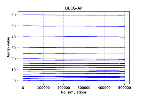
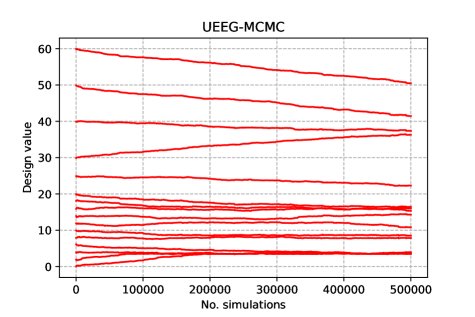
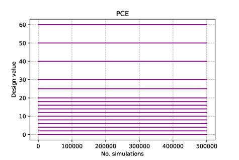
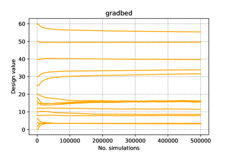
Figure B.4: Convergence of the individual design dimensions for STAT5 model with additive noise $\mathcal{N}(0,0.001)$.

References

- Abadi (2016) Abadi, M. 2016. TensorFlow: learning functions at scale. In Proceedings of the 21st ACM SIGPLAN International Conference on Functional Programming, 1–1.
- Ahmed and Gokhale (1989) Ahmed, N. A.; and Gokhale, D. 1989. Entropy expressions and their estimators for multivariate distributions. IEEE Transactions on Information Theory, 35(3): 688–692.
- Alemi et al. (2016) Alemi, A. A.; Fischer, I.; Dillon, J. V.; and Murphy, K. 2016. Deep variational information bottleneck. arXiv preprint arXiv:1612.00410.
- Ao and Li (2020) Ao, Z.; and Li, J. 2020. An approximate KLD based experimental design for models with intractable likelihoods. In International Conference on Artificial Intelligence and Statistics, 3241–3251. PMLR.
- Banga and Balsa-Canto (2008) Banga, J. R.; and Balsa-Canto, E. 2008. Parameter estimation and optimal experimental design. Essays in biochemistry, 45: 195–210.
- Barber and Agakov (2004) Barber, D.; and Agakov, F. 2004. The im algorithm: a variational approach to information maximization. Advances in neural information processing systems, 16(320): 201.
- Belghazi et al. (2018) Belghazi, M. I.; Baratin, A.; Rajeshwar, S.; Ozair, S.; Bengio, Y.; Courville, A.; and Hjelm, D. 2018. Mutual information neural estimation. In International conference on machine learning, 531–540. PMLR.
- Bishop (1994) Bishop, C. M. 1994. Mixture density networks.
- Borth (1975) Borth, D. M. 1975. A total entropy criterion for the dual problem of model discrimination and parameter estimation. Journal of the Royal Statistical Society: Series B (Methodological), 37(1): 77–87.
- Brehmer et al. (2020) Brehmer, J.; Louppe, G.; Pavez, J.; and Cranmer, K. 2020. Mining gold from implicit models to improve likelihood-free inference. Proceedings of the National Academy of Sciences, 117(10): 5242–5249.
- Butcher (1996) Butcher, J. C. 1996. A history of Runge-Kutta methods. Applied numerical mathematics, 20(3): 247–260.
- Chen et al. (2018) Chen, R. T. Q.; Rubanova, Y.; Bettencourt, J.; and Duvenaud, D. 2018. Neural Ordinary Differential Equations. Advances in Neural Information Processing Systems.
- Cover (1999) Cover, T. M. 1999. Elements of information theory. John Wiley & Sons.
- Donsker and Varadhan (1975) Donsker, M. D.; and Varadhan, S. S. 1975. Asymptotic evaluation of certain Markov process expectations for large time, I. Communications on Pure and Applied Mathematics, 28(1): 1–47.
- Feng and Li (2022) Feng, R.; and Li, P. 2022. Sample recycling method–a new approach to efficient nested Monte Carlo simulations. Insurance: Mathematics and Economics, 105: 336–359.
- Foster et al. (2019) Foster, A.; Jankowiak, M.; Bingham, E.; Horsfall, P.; Teh, Y. W.; Rainforth, T.; and Goodman, N. 2019. Variational Bayesian optimal experimental design. Advances in Neural Information Processing Systems, 32.
- Foster et al. (2020) Foster, A.; Jankowiak, M.; O’Meara, M.; Teh, Y. W.; and Rainforth, T. 2020. A unified stochastic gradient approach to designing bayesian-optimal experiments. In International Conference on Artificial Intelligence and Statistics, 2959–2969. PMLR.
- Goda et al. (2022) Goda, T.; Hironaka, T.; Kitade, W.; and Foster, A. 2022. Unbiased MLMC stochastic gradient-based optimization of Bayesian experimental designs. SIAM Journal on Scientific Computing, 44(1): A286–A311.
- Huan and Marzouk (2013) Huan, X.; and Marzouk, Y. M. 2013. Simulation-based optimal Bayesian experimental design for nonlinear systems. Journal of Computational Physics, 232(1): 288–317.
- Hyvärinen and Dayan (2005) Hyvärinen, A.; and Dayan, P. 2005. Estimation of non-normalized statistical models by score matching. Journal of Machine Learning Research, 6(4).
- Kleinegesse and Gutmann (2019) Kleinegesse, S.; and Gutmann, M. U. 2019. Efficient Bayesian experimental design for implicit models. In The 22nd International Conference on Artificial Intelligence and Statistics, 476–485. PMLR.
- Kleinegesse and Gutmann (2020) Kleinegesse, S.; and Gutmann, M. U. 2020. Bayesian experimental design for implicit models by mutual information neural estimation. In International Conference on Machine Learning, 5316–5326. PMLR.
- Kleinegesse and Gutmann (2021) Kleinegesse, S.; and Gutmann, M. U. 2021. Gradient-based Bayesian experimental design for implicit models using mutual information lower bounds. arXiv preprint arXiv:2105.04379.
- Kraskov, Stögbauer, and Grassberger (2004) Kraskov, A.; Stögbauer, H.; and Grassberger, P. 2004. Estimating mutual information. Physical review E, 69(6): 066138.
- Kreutz and Timmer (2009) Kreutz, C.; and Timmer, J. 2009. Systems biology: experimental design. The FEBS journal, 276(4): 923–942.
- Lewi, Butera, and Paninski (2009) Lewi, J.; Butera, R.; and Paninski, L. 2009. Sequential optimal design of neurophysiology experiments. Neural computation, 21(3): 619–687.
- Li and Turner (2017) Li, Y.; and Turner, R. E. 2017. Gradient estimators for implicit models. arXiv preprint arXiv:1705.07107.
- Lim et al. (2020) Lim, J. H.; Courville, A.; Pal, C.; and Huang, C.-W. 2020. AR-DAE: towards unbiased neural entropy gradient estimation. In International Conference on Machine Learning, 6061–6071. PMLR.
- Long et al. (2013) Long, Q.; Scavino, M.; Tempone, R.; and Wang, S. 2013. Fast estimation of expected information gains for Bayesian experimental designs based on Laplace approximations. Computer Methods in Applied Mechanics and Engineering, 259: 24–39.
- Lyu et al. (2019) Lyu, J.; Wang, S.; Balius, T. E.; Singh, I.; Levit, A.; Moroz, Y. S.; O’Meara, M. J.; Che, T.; Algaa, E.; Tolmachova, K.; et al. 2019. Ultra-large library docking for discovering new chemotypes. Nature, 566(7743): 224–229.
- Melendez et al. (2021) Melendez, J.; Furnstahl, R.; Grießhammer, H.; McGovern, J.; Phillips, D.; and Pratola, M. 2021. Designing optimal experiments: an application to proton Compton scattering. The European Physical Journal A, 57: 1–24.
- Mohamed et al. (2020) Mohamed, S.; Rosca, M.; Figurnov, M.; and Mnih, A. 2020. Monte carlo gradient estimation in machine learning. The Journal of Machine Learning Research, 21(1): 5183–5244.
- Müller (2005) Müller, P. 2005. Simulation based optimal design. Handbook of Statistics, 25: 509–518.
- Neal (2003) Neal, R. M. 2003. Slice sampling. The annals of statistics, 31(3): 705–767.
- Nelder and Mead (1965) Nelder, J. A.; and Mead, R. 1965. A simplex method for function minimization. The computer journal, 7(4): 308–313.
- Nguyen, Wainwright, and Jordan (2010) Nguyen, X.; Wainwright, M. J.; and Jordan, M. I. 2010. Estimating divergence functionals and the likelihood ratio by convex risk minimization. IEEE Transactions on Information Theory, 56(11): 5847–5861.
- Oord, Li, and Vinyals (2018) Oord, A. v. d.; Li, Y.; and Vinyals, O. 2018. Representation learning with contrastive predictive coding. arXiv preprint arXiv:1807.03748.
- Papamakarios et al. (2021) Papamakarios, G.; Nalisnick, E.; Rezende, D. J.; Mohamed, S.; and Lakshminarayanan, B. 2021. Normalizing flows for probabilistic modeling and inference. The Journal of Machine Learning Research, 22(1): 2617–2680.
- Paszke et al. (2017) Paszke, A.; Gross, S.; Chintala, S.; Chanan, G.; Yang, E.; DeVito, Z.; Lin, Z.; Desmaison, A.; Antiga, L.; and Lerer, A. 2017. Automatic differentiation in pytorch.
- Peifer and Timmer (2007) Peifer, M.; and Timmer, J. 2007. Parameter estimation in ordinary differential equations for biochemical processes using the method of multiple shooting. IET systems biology, 1(2): 78–88.
- Poole et al. (2019) Poole, B.; Ozair, S.; Van Den Oord, A.; Alemi, A.; and Tucker, G. 2019. On variational bounds of mutual information. In International Conference on Machine Learning, 5171–5180. PMLR.
- Rainforth et al. (2018) Rainforth, T.; Cornish, R.; Yang, H.; Warrington, A.; and Wood, F. 2018. On nesting monte carlo estimators. In International Conference on Machine Learning, 4267–4276. PMLR.
- Rainforth et al. (2023) Rainforth, T.; Foster, A.; Ivanova, D. R.; and Smith, F. B. 2023. Modern bayesian experimental design. arXiv preprint arXiv:2302.14545.
- Rhee and Glynn (2015) Rhee, C.-h.; and Glynn, P. W. 2015. Unbiased estimation with square root convergence for SDE models. Operations Research, 63(5): 1026–1043.
- Ryan et al. (2016) Ryan, E. G.; Drovandi, C. C.; McGree, J. M.; and Pettitt, A. N. 2016. A review of modern computational algorithms for Bayesian optimal design. International Statistical Review, 84(1): 128–154.
- Ryan et al. (2014) Ryan, E. G.; Drovandi, C. C.; Thompson, M. H.; and Pettitt, A. N. 2014. Towards Bayesian experimental design for nonlinear models that require a large number of sampling times. Computational Statistics & Data Analysis, 70: 45–60.
- Ryan (2003) Ryan, K. J. 2003. Estimating expected information gains for experimental designs with application to the random fatigue-limit model. Journal of Computational and Graphical Statistics, 12(3): 585–603.
- Seeger and Nickisch (2008) Seeger, M. W.; and Nickisch, H. 2008. Compressed sensing and Bayesian experimental design. In Proceedings of the 25th international conference on Machine learning, 912–919.
- Shi, Sun, and Zhu (2018) Shi, J.; Sun, S.; and Zhu, J. 2018. A spectral approach to gradient estimation for implicit distributions. In International Conference on Machine Learning, 4644–4653. PMLR.
- Snoek, Larochelle, and Adams (2012) Snoek, J.; Larochelle, H.; and Adams, R. P. 2012. Practical bayesian optimization of machine learning algorithms. Advances in neural information processing systems, 25.
- Song and Ermon (2019) Song, J.; and Ermon, S. 2019. Understanding the limitations of variational mutual information estimators. arXiv preprint arXiv:1910.06222.
- Song et al. (2020) Song, Y.; Garg, S.; Shi, J.; and Ermon, S. 2020. Sliced score matching: A scalable approach to density and score estimation. In Uncertainty in Artificial Intelligence, 574–584. PMLR.
- Spall (1998) Spall, J. C. 1998. An overview of the simultaneous perturbation method for efficient optimization. Johns Hopkins apl technical digest, 19(4): 482–492.
- Swameye et al. (2003) Swameye, I.; Müller, T.; Timmer, J.; Sandra, O.; and Klingmüller, U. 2003. Identification of nucleocytoplasmic cycling as a remote sensor in cellular signaling by databased modeling. Proceedings of the National Academy of Sciences, 100(3): 1028–1033.
- Thomas et al. (2022) Thomas, O.; Dutta, R.; Corander, J.; Kaski, S.; and Gutmann, M. U. 2022. Likelihood-free inference by ratio estimation. Bayesian Analysis, 17(1): 1–31.
- Tsilifis, Ghanem, and Hajali (2017) Tsilifis, P.; Ghanem, R. G.; and Hajali, P. 2017. Efficient Bayesian experimentation using an expected information gain lower bound. SIAM/ASA Journal on Uncertainty Quantification, 5(1): 30–62.
- Wen et al. (2021) Wen, L.; Bai, H.; He, L.; Zhou, Y.; Zhou, M.; and Xu, Z. 2021. Gradient estimation of information measures in deep learning. Knowledge-Based Systems, 224: 107046.
- Zaballa and Hui (2023) Zaballa, V. D.; and Hui, E. E. 2023. Stochastic Gradient Bayesian Optimal Experimental Designs for Simulation-based Inference. arXiv preprint arXiv:2306.15731.
- Zhang, Bi, and Zhang (2021) Zhang, J.; Bi, S.; and Zhang, G. 2021. A scalable gradient free method for bayesian experimental design with implicit models. In International Conference on Artificial Intelligence and Statistics, 3745–3753. PMLR.
- Zhang et al. (2022) Zhang, K.; Feng, B. M.; Liu, G.; and Wang, S. 2022. Sample Recycling for Nested Simulation with Application in Portfolio Risk Measurement. arXiv preprint arXiv:2203.15929.